variations of topside n(h)-profiles of the ionosphere during space weather...

VARIATIONS OF TOPSIDE N(h)-PROFILES OF THE IONOSPHERE

DURING SPACE WEATHER EVENTS

O.A. Maltseva, G.A. Zbankov, N.S. Mozhaeva, T.V. Nikitenko

Institute for Physics, Southern Federal University, Rostov-on-Don, 344090, Russia, e-mail:

[email protected]

Abstract. Space Weather effects are well studied in the behavior of such ionospheric parameters as the critical frequency foF2, the maximum height hmF2, the total electron content TEC not in the behavior of N(h)-profiles. Moreover, the behavior of N(h)-profiles are well known for the bottom side of the ionosphere, but not for the topside one, and certainly not for disturbed conditions. In this paper it is proposed to use a new model IRI2010 (IRI-Plas) and its additional adaptation to the plasma frequency of satellites to determine the variations of N(h)-profiles. It allows us to estimate effects of Space Weather in all heights up to altitudes of navigation satellites. Two types of response of the bottom and topside ionosphere to disturbances are discovered: synchronous and asynchronous.

INTRODUCTION Modern communication systems, systems of navigation and positioning are known to operate in near space. To describe the state of the space a special term is used: “Space Weather”. The general definition of space weather is solar-terrestrial relations. The specific meaning is the state of the ionosphere and magnetosphere. Space Weather effects are well studied in the behavior of such ionospheric parameters as the critical frequency foF2, the maximum height hmF2, the total electron content TEC not in the behavior of N(h)-profiles. Moreover, the behavior of N(h)-profiles are well known for the bottom side ionosphere, but not for the topside one, and certainly not for disturbed conditions. There are a lot of models of the ionosphere: 1) physical (theoretical), 2) parametric, 3) empirical (e.g. Feltens et al., 2011). But when describing the state of the ionosphere in practical applications really only the empirical models are used. This paper proposes to use a new model IRI2010 (IRI-Plas) (Gulyaeva, 2003, 2011) and its additional adaptation to the plasma frequency of satellites to determine the variations of N(h)-profiles during Space Weather events. ADVANTAGES OF THE IRI-PLAS MODEL

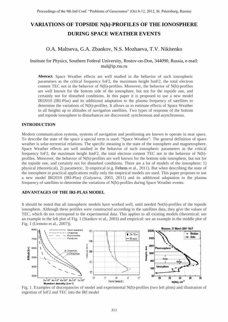
It should be noted that all ionospheric models have worked well, until needed Ne(h)-profiles of the topside ionosphere. Although these profiles were constructed according to the satellites data, they give the values of TEC, which do not correspond to the experimental data. This applies to all existing models (theoretical: see an example in the left plot of Fig. 1 (Stankov et al., 2003) and empirical: see an example in the middle plot of Fig. 1 (Uemoto et al., 2007)).

Fig. 1. Examples of discrepancies of model and experimental N(h)-profiles (two left plots) and illustration of ingestion of foF2 and TEC into the IRI model

Proceedings of the 9th Intl Conf. “Problems of Geocosmos” (Oct 8-12, 2012, St. Petersburg, Russia)

311

The advantages of the IRI-Plas model are: 1) the development of parameters of the topside part of Ne(h)-profile, 2) consideration of the plasmaspheric part of the magnetosphere, 3) adaptation of the model to experimental data of the TEC. The topside Ne(h)-profile is determined by the scale parameter Hsc (the right part of Fig. 1 (Gulyaeva, 2011)). It is the distance above the peak height between the height where Ne decays by a factor “e” and the peak height. The height hsc serves as a boundary for merging the IRI topside profile with the plasmasphere. Ingestion of the experimental TEC into the model gives the instantaneous value Hosc instead of the median value Hmsc. Of course, there are some plasmaspheric models. Comparison of results for two models (IRI and GCPM) with experiments showed the best agreement with the IRI-Plas (Gulyaeva and Gallagher, 2007). GCPM-2000 is the Global Core Plasma Model of Gallagher. WHAT ARE THE POSSIBILITIES TO DETERMINE THE N(H)-PROFILE?

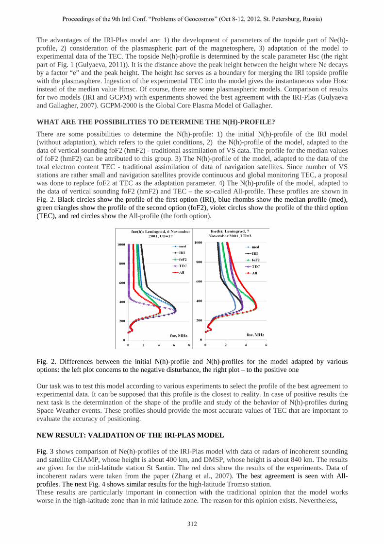
There are some possibilities to determine the N(h)-profile: 1) the initial N(h)-profile of the IRI model (without adaptation), which refers to the quiet conditions, 2) the N(h)-profile of the model, adapted to the data of vertical sounding foF2 (hmF2) - traditional assimilation of VS data. The profile for the median values of foF2 (hmF2) can be attributed to this group. 3) The N(h)-profile of the model, adapted to the data of the total electron content TEC - traditional assimilation of data of navigation satellites. Since number of VS stations are rather small and navigation satellites provide continuous and global monitoring TEC, a proposal was done to replace foF2 at TEC as the adaptation parameter. 4) The N(h)-profile of the model, adapted to the data of vertical sounding foF2 (hmF2) and TEC – the so-called All-profile. These profiles are shown in Fig. 2. Black circles show the profile of the first option (IRI), blue rhombs show the median profile (med), green triangles show the profile of the second option (foF2), violet circles show the profile of the third option (TEC), and red circles show the All-profile (the forth option).

Fig. 2. Differences between the initial N(h)-profile and N(h)-profiles for the model adapted by various options: the left plot concerns to the negative disturbance, the right plot – to the positive one Our task was to test this model according to various experiments to select the profile of the best agreement to experimental data. It can be supposed that this profile is the closest to reality. In case of positive results the next task is the determination of the shape of the profile and study of the behavior of N(h)-profiles during Space Weather events. These profiles should provide the most accurate values of TEC that are important to evaluate the accuracy of positioning. NEW RESULT: VALIDATION OF THE IRI-PLAS MODEL Fig. 3 shows comparison of Ne(h)-profiles of the IRI-Plas model with data of radars of incoherent sounding and satellite CHAMP, whose height is about 400 km, and DMSP, whose height is about 840 km. The results are given for the mid-latitude station St Santin. The red dots show the results of the experiments. Data of incoherent radars were taken from the paper (Zhang et al., 2007). The best agreement is seen with All-profiles. The next Fig. 4 shows similar results for the high-latitude Tromso station. These results are particularly important in connection with the traditional opinion that the model works worse in the high-latitude zone than in mid latitude zone. The reason for this opinion exists. Nevertheless,


312

Fig. 3. Results of testing the IRI-Plas model by data of ISR and satellites CHAMP and DMSP for the middle latitude StSantin station


313

Fig. 4. Results of testing the IRI-Plas model by data of ISR and satellites CHAMP and DMSP for the high latitude Tromso station the results of comparison are not worse than for the mid-latitudes. In the same time, these plots consisting of results for various global TEC maps (JPL, CODE, UPC, ESA) show that N(h)-profiles can be strongly differed. That is why the given paper proposes an additional adaptation to the values of the plasma frequency fne on the heights of different satellites to select the N(h)-profile. FEATURES OF IONOSPHERIC N(h)-PROFILES RESPONSE TO SPACE WEATHER DISTURBANCES It is well known the behavior of such ionospheric parameters as foF2, hmF2, TEC during disturbances. Adaptation of the model to disturbed values of parameters allows us to determine features of ionospheric N(h)-profiles response to Space Weather disturbances. The specific attention was paid to the search of cases of asynchronous response of the bottom and topside ionosphere to disturbances because these cases don’t allow us to use the median slab thickness to determine NmF2 from TEC (Maltseva et al. 2012).

Fig. 5. Illustration of the response of N(h)-profiles in cases of: a) negative disturbances, b) positive disturbances, c) constancy of foF2, d) different reaction of two parts of the ionosphere It was discovered some typical cases illustrated in Fig. 5: 1) synchronous decrease of the ionization in both of parts of the ionosphere during negative disturbances (Fig. 5a), 2) synchronous increase of the ionization in both of parts of the ionosphere during positive disturbances (Fig. 5b), 2) increase (or decrease) of the ionization in both of parts when foF2 don’t change (Fig. 5c), 4) asynchronous response (Fig. 5d). Determination of such profiles allows us to estimate effects of Space Weather in all heights up to altitudes of navigation satellites.


314

NEW RESULT: BEHAVIOR OF N(h)-PROFILES IN THE CHAIN OF STATIONS IN APRIL 2001 A chain of ground ionosondes consisting of Loparsk, Leningrad, Moscow, Rostov was selected. We use an example of April 2001, including two strong disturbances (1-2.04, a minimum Dst = -228 nT, 11-12.04, the minimum Dst = -271 nT) and two weak disturbances (18, 22-23.04) with a minimum of Dst ~ -100 nT. Behavior of N(h)-profiles are shown in Fig. 6, variations of them – in Fig. 7.

Fig. 6. Behavior of N(h)-profiles in the chain of stations during day and night

Fig. 7. Deviations of disturbed profiles of Fig. 6 from profiles of quiet conditions Quantitative details are as following. Variations were estimated as deviations of disturbed profiles from the monthly median ones. It was detected nine cases of travelling satellites over all the stations, which allows us to estimate the latitudinal profiles. These passages were near noon and midnight, and covered both positive disturbance (1-6.04) and negative (all other) ones. The strongest variations were found for profiles of the Leningrad station, apparently as a result of its position near the projection of the "quiet" plasmapause. In the daytime, during the positive disturbance enhancing of concentration reached 5-15% at all altitudes, increasing with latitude. On April 12 at UT = 13 at the Leningrad station, deviations were -75% providing a deep minimum of the latitude dependence. On April 20 N(h)-profiles had 5-10% gain in the bottom side and a similar weakening - at the topside. On April 28 at the Rostov station, the lowest concentration of N(h)-profiles was at the bottom side and a 20% gain at the topside. At night, 1-2.04 at UT = 23-1 the Leningrad station was in zone of a strong increase of the ionization (40%) with a concentration exceeding the concentration of the other stations at all altitudes. This provided the location of the Moscow station in the zone of trough. On April 6-7 at UT = 23-1, N(h)-profiles of Loparsk and Moscow were still in the area of the


315

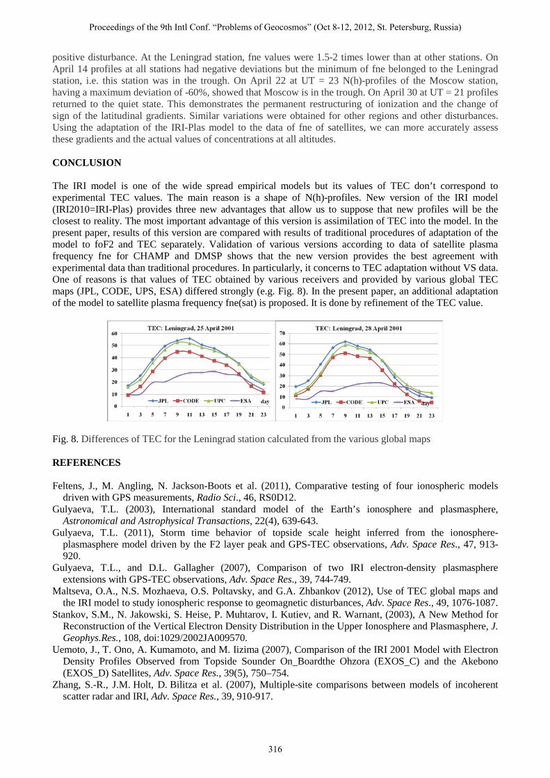
positive disturbance. At the Leningrad station, fne values were 1.5-2 times lower than at other stations. On April 14 profiles at all stations had negative deviations but the minimum of fne belonged to the Leningrad station, i.e. this station was in the trough. On April 22 at UT = 23 N(h)-profiles of the Moscow station, having a maximum deviation of -60%, showed that Moscow is in the trough. On April 30 at UT = 21 profiles returned to the quiet state. This demonstrates the permanent restructuring of ionization and the change of sign of the latitudinal gradients. Similar variations were obtained for other regions and other disturbances. Using the adaptation of the IRI-Plas model to the data of fne of satellites, we can more accurately assess these gradients and the actual values of concentrations at all altitudes. CONCLUSION The IRI model is one of the wide spread empirical models but its values of TEC don’t correspond to experimental TEC values. The main reason is a shape of N(h)-profiles. New version of the IRI model (IRI2010=IRI-Plas) provides three new advantages that allow us to suppose that new profiles will be the closest to reality. The most important advantage of this version is assimilation of TEC into the model. In the present paper, results of this version are compared with results of traditional procedures of adaptation of the model to foF2 and TEC separately. Validation of various versions according to data of satellite plasma frequency fne for CHAMP and DMSP shows that the new version provides the best agreement with experimental data than traditional procedures. In particularly, it concerns to TEC adaptation without VS data. One of reasons is that values of TEC obtained by various receivers and provided by various global TEC maps (JPL, CODE, UPS, ESA) differed strongly (e.g. Fig. 8). In the present paper, an additional adaptation of the model to satellite plasma frequency fne(sat) is proposed. It is done by refinement of the TEC value.

Fig. 8. Differences of TEC for the Leningrad station calculated from the various global maps REFERENCES Feltens, J., M. Angling, N. Jackson-Boots et al. (2011), Comparative testing of four ionospheric models

driven with GPS measurements, Radio Sci., 46, RS0D12. Gulyaeva, T.L. (2003), International standard model of the Earth’s ionosphere and plasmasphere,

Astronomical and Astrophysical Transactions, 22(4), 639-643. Gulyaeva, T.L. (2011), Storm time behavior of topside scale height inferred from the ionosphere-

plasmasphere model driven by the F2 layer peak and GPS-TEC observations, Adv. Space Res., 47, 913-920.

Gulyaeva, T.L., and D.L. Gallagher (2007), Comparison of two IRI electron-density plasmasphere extensions with GPS-TEC observations, Adv. Space Res., 39, 744-749.

Maltseva, O.A., N.S. Mozhaeva, O.S. Poltavsky, and G.A. Zhbankov (2012), Use of TEC global maps and the IRI model to study ionospheric response to geomagnetic disturbances, Adv. Space Res., 49, 1076-1087.

Stankov, S.M., N. Jakowski, S. Heise, P. Muhtarov, I. Kutiev, and R. Warnant, (2003), A New Method for Reconstruction of the Vertical Electron Density Distribution in the Upper Ionosphere and Plasmasphere, J. Geophys.Res., 108, doi:1029/2002JA009570.

Uemoto, J., T. Ono, A. Kumamoto, and M. Iizima (2007), Comparison of the IRI 2001 Model with Electron Density Profiles Observed from Topside Sounder On_Boardthe Ohzora (EXOS_C) and the Akebono (EXOS_D) Satellites, Adv. Space Res., 39(5), 750–754.

Zhang, S.-R., J.M. Holt, D. Bilitza et al. (2007), Multiple-site comparisons between models of incoherent scatter radar and IRI, Adv. Space Res., 39, 910-917.


316

variations of topside n(h)-profiles of the ionosphere during space weather...

Documents