variational viewpoint of the quadratic markov measure field models

1

Variational Viewpoint of the Quadratic MarkovMeasure Field Models: Theory and Algorithms

Mariano Rivera and Oscar Dalmau

Abstract—We present a framework for image segmentation based on quadratic programing; i.e. by the minimization of a quadraticregularized energy linearly constrained. In particular, we present a new variational derivation of the Quadratic Makov Measure Field(QMMF) models that can be understood as a procedure for regularizing the model preferences (memberships or likelihood). Wealso present efficient optimization algorithms. In the QMMFs the uncertainty in the computed regularized probability measure field iscontrolled by penalizing the Gini’s coefficient and hence it affects the convexity of the QP problem. The convex case is reduced tothe solution of a positive definite linear system and, for that case, an efficient Gauss–Seidel scheme is presented. On the other hand,we present a efficient Projected Gauss-Seidel with a subspace minimization for optimizing the non–convex case. We demonstrate theproposal capabilities by experiments and numerical comparisons with interactive two-class segmentation as well as in the simultaneousestimation of segmentation and (parametric and non-parametric) generative models. We present extensions to the original formulationfor including color and texture clues as well as imprecise user scibbles in an interactive framework.

Index Terms—Image segmentation, Quadratic programming, Interactive segmentation, Computer vision, Markov random fields,Information measures, Subspace minimization.

F

1 INTRODUCTION

IMAGE SEGMENTATION is an active research topic incomputer vision and image analysis. It is a core pro-

cess in many practical applications, see for instance thelisted in [1]. Image segmentation is an ill–posed problemthat is task and user dependent; this is illustrated by thethree possible segmentation of a single scene in Fig. 1.Among many approaches, methods based on MarkovRandom Field (MRF) models have become popular fordesigning segmentation algorithms because their flexi-bility for being adapted to very different circumstancesas: color, connected components, motion, stereo dispar-ity, etc.; as for example: [1], [2], [3], [4], [5], [6].

The MRFs approach allows one to express the label as-signment problem into an energy function that includesspatial context information for each pixel and thuspromotes smooth segmentations. The energy functioncodifies the compromise of assigning a label to a pixel bydepending on the value of the particular pixel and thevalue of the surrounding pixels. Since the label space isdiscrete, frequently, the segmentation problem requiresof the solution of a combinatorial (integer) optimiza-tion problem. In that order, max–flow/graph–cut basedtechniques are among the most successful optimization

• Copyright (c) 2010 IEEE. Personal use of this material is permitted.However, permission to use this material for any other purposes must beobtained from the IEEE by sending a request to [email protected].

• The authors are with the Department of Computer Science, Centro deInvestigacion en Matematicas AC , Guanajuato, GTO, Mexico 36000.E-mail: [email protected], see http://www.cimat.mx/˜mrivera.html

The authors thank to the anonymous reviewers for their comments that helpto improve the quality of the paper.This work is supported by CONACYT, Mexico (Grants 61367 and 131369).O. Dalmau was supported by a CIMAT AND CONACYT scholarships.

1

Variational Viewpoint of the Quadratic MarkovMeasure Field Models: Theory and Algorithms

Mariano Rivera and Oscar Dalmau

Abstract—We present a framework for image segmentation based on quadratic programing; i.e. by the minimization of a quadraticregularized energy linearly constrained. In particular, we present a new variational derivation of the Quadratic Makov Measure Field(QMMF) models that can be understood as a procedure for regularizing the model preferences (memberships or likelihood). Wealso present efficient optimization algorithms. In the QMMFs the uncertainty in the computed regularized probability measure field iscontrolled by penalizing the Gini’s coefficient and hence it affects the convexity of the QP problem. The convex case is reduced tothe solution of a positive definite linear system and, for that case, an efficient Gauss–Seidel scheme is presented. On the other hand,we present a efficient Projected Gauss-Seidel with a subspace minimization for optimizing the non–convex case. We demonstrate theproposal capabilities by experiments and numerical comparisons with interactive two-class segmentation as well as in the simultaneousestimation of segmentation and (parametric and non-parametric) generative models. We present extensions to the original formulationfor including color and texture clues as well as imprecise user scibbles in an interactive framework.

Index Terms—Image segmentation, Quadratic programming, Interactive segmentation, Computer vision, Markov random fields,Information measures, Subspace minimization.

F

1 INTRODUCTION

IMAGE SEGMENTATION is an active research topic incomputer vision and image analysis. It is a core pro-

cess in many practical applications, see for instance thelisted in [1]. Image segmentation is an ill–posed problemthat is task and user dependent; this is illustrated by thethree possible segmentation of a single scene in Fig. 1.Among many approaches, methods based on MarkovRandom Field (MRF) models have become popular fordesigning segmentation algorithms because their flexi-bility for being adapted to very different circumstancesas: color, connected components, motion, stereo dispar-ity, etc.; as for example: [1], [2], [3], [4], [5], [6].

The MRFs approach allows one to express the label as-signment problem into an energy function that includesspatial context information for each pixel and thuspromotes smooth segmentations. The energy functioncodifies the compromise of assigning a label to a pixel bydepending on the value of the particular pixel and thevalue of the surrounding pixels. Since the label space isdiscrete, frequently, the segmentation problem requiresof the solution of a combinatorial (integer) optimiza-tion problem. In that order, max–flow/graph–cut basedtechniques are among the most successful optimizationalgorithms [7], [8], [9], [10], [11]. In particular, graph-cut based methods can solve the binary (two labels)segmentation problem in polynomial time [5]. The search

• The authors are with the Department of Computer Science, Centro deInvestigacion en Matematicas AC , Guanajuato, GTO, Mexico 36000.E-mail: [email protected], see http://www.cimat.mx/˜mrivera.html

The authors thank to the anonymous reviewers for their comments that helpto improve the quality of the paper.This work is supported by CONACYT, Mexico (Grants 61367 and 131369).O. Dalmau was supported by a CIMAT AND CONACYT scholarships.

Fig. 1. Multi–class segmentation of a same scene ac-cording to different criteria (codified in the user scrib-bles). The columns correspond to segmentations by color,semantic objects and planar regions, respectively. Thesegmentation were computed with the multi-class EC–QMMF algorithm using color histograms, see section 5.1.

for faster algorithms is, indeed, an active research topic.Recently, some authors have reported advances in the so-lution of the multi-label problem. Their strategy consistsin constructing an approximated problem by relaxing theinteger constraint [12], [13]. Additionally, there are twoimportant issues in discrete MRFs: the reuse of solutionsin the case of dynamic MRFs [8], [14] and to measure theuncertainty in the label assignement [14].

However, the combinatorial approach (hard segmen-tation) is neither the most computationally efficientnor, in some cases, the most precise strategy for solv-ing the segmentation problem. A different approachis to directly estimate the uncertainties on the labelassignment (memberships) [1], [4], [6], [15], [16]. In theBayesian framework, such memberships can naturally

Fig. 1. Multi–class segmentation of a same scene ac-cording to different criteria (codified in the user scrib-bles). The columns correspond to segmentations by color,semantic objects and planar regions, respectively. Thesegmentation were computed with the multi-class EC–QMMF algorithm using color histograms, see section 5.1.

algorithms [7], [8], [9], [10], [11]. In particular, graph-cut based methods can solve the binary (two labels)segmentation problem in polynomial time [5]. The searchfor faster algorithms is, indeed, an active research topic.Recently, some authors have reported advances in the so-lution of the multi-label problem. Their strategy consistsin constructing an approximated problem by relaxing theinteger constraint [12], [13]. Additionally, there are twoimportant issues in discrete MRFs: the reuse of solutionsin the case of dynamic MRFs [8], [14] and to measure theuncertainty in the label assignement [14].

However, the combinatorial approach (hard segmen-tation) is neither the most computationally efficientnor, in some cases, the most precise strategy for solv-ing the segmentation problem. A different approach

2

is to directly estimate the uncertainties on the labelassignment (memberships) [1], [4], [6], [15], [16]. In theBayesian framework, such memberships can naturallybe expressed in terms of probabilities—leading to thenamed probabilistic segmentation (PS) methods.

In this work, we present new theoretical insights,extensions and computational efficient algorithms to therecently reported PS method named Quadratic MarkovMeasure Field (QMMF) models [1]. In particular, wedemonstrate that the data term (potential) in QMMFs is adissimilarity measure between discrete density distribu-tions and satisfies the here proposed design guidelinesfor PS methods. We also present efficient optimizationalgorithms proper for the two-classes (binary) and multi-classes segmentation problems. We demonstrate that thesolution to a convex QMMF is computed by solvinga linear system. On the other hand, since the entropycontrol proposed in Ref. [1] affects the convexity of thequadratic programing problem, then we propose a pro-jection strategy combined with a subspace minimizationmethod for the nonconvex QMMF case [17]. In addition,we include extensions to the QMMF framework thatwiden its capabilities.

Preliminary results of this work were reported in [18],[19], [20], [21]. We organize the paper as follows. In orderto make this paper self contained, Section 2 shows a briefreview of the original Bayesian derivation of the QMMFmodels. Section 3 presents a new variational justifica-tion of the QMMF models. The new QMMF viewpointshows that the data term is a dissimilarity measure (aninformation measure) between discrete density distribu-tions that preserves class preferences. Additionally, thepresented framework demonstrates that the low entropyrequirement (used in the original derivation [1]) is not aconstraint in the QMMF models. Section 4 presents newefficient optimization algorithms. Then, experiments thatdemonstrate the method performance are presented inSection 5. Finally, our conclusions are given in Section 6.

2 BRIEF REVIEW OF ENTROPY–CONTROLLEDQUADRATIC MARKOV MEASURE FIELD MOD-ELS: THE BAYESIAN DERIVATION

First we introduce the notation used in this paper. Wedenote by r a pixel position in the image. Let L = r bethe set of sites of a regular lattice that defines the image,then R ⊆ L denotes the region of interest. Moreover,K = 1, . . . ,K denotes the set of index classes and

SK = z ∈ RK | 1T z = 1, z 0 (1)

is the simplex whose elements are probability measures;where the vector 1 has all its entries equal to one andits size is defined by the context. In our notation, givenz ∈ RK then z 0 ⇐⇒ zk ≥ 0 for k = 1, 2, . . . ,K.

Recently, in Ref. [1] the Entropy Controlled QuadraticMarkov Measure Field (EC-QMMF) models for imagemulticlass segmentation were proposed. Such models are

computationally efficient and produce Probabilistic Seg-mentations of excellent quality. Whereas hard segmen-tation procedures compute a hard label for each pixel,PS approaches (as QMMFs) compute the confidence ofassigning a particular label to each pixel. In the Bayesianframework, the amount of confidence (or uncertainty) isrepresented in terms of probabilities. In that frameworkpk(r) denotes the unknown probability of the pixel r ∈ Rto belong to the class k ∈ K. Such a vector field p is aprobability measure field; i.e., p(r) ∈ SK .

The QMMF formulation constructs on the generativemodel:

g(r) = p(r)T I(r) + η(r) (2)

where g is the observed image, the images vector I =[I1, I2, . . . , IK ]T is generated with a parametric model setΦ with parameters θ. Then we use indistinctly Ik(r) orΦ(r, θk) for the r–pixel–value in the kth image model;where the parameters θ = θk,∀k, are known or esti-mated. A simple example of model is Φ(r; θk) = θk+η(r).In such a case the image regions are constant planesdefined by the scalar θk. In addition, η is a possible noise(or residual) and the probability measure p(r) can beunderstood as a matting vector [1], [16].

In the original proposal, the QMMF models are de-rived from the observation model (2), assuming i.i.d.Gaussian noise (with zero mean and standard deviationσ) and measure vectors p(r) with neglected entropy;i.e., the product pk(r)pl(r) ≈ 0 for k 6= l at any pixelr [1]. Hence in the Bayesian regularization framework,the conditional probability of the observation given thematting factors and the image–models is given by:

P (g|p, θ) ∝ exp

[− 1

2σ2

∑

r

‖g(r)− p(r)TΦ(r, θk)‖2]

(3)

≈ exp

[∑

r

p(r)TDrp(r)

](4)

where the approximation (4) is valid in the low–entropylimit;

Drdef= diag( − log v(r, θ)) (5)

is a diagonal matrix associated with the pixel r. More-over, vk(r, θ) ∈ SK is the normalized probability measurevector

vk(r, θ) ∝ exp

[− 1

2σ2‖g(r)− Φ(r, θk)‖2

](6)

where the vector v is the normalized version of the vectorv: the preferences of the data for the image–models; thisleads us to the next definition:

Definition The likelihood (model preference) vk(r, θ) isthe conditional probability of observing a particular pixelvalue g(r) by assuming that such a pixel is taken fromthe image Ik:

vk(r, θ)def= P (g(r)|p(r) = ek,Φ(r, θk))), (7)

3

where ek is the kth canonical basis vector.

Last derivation is based on the assumption of Gaussiannoise η. The generalization to other distributions, differ-ent from the Gaussian, is justified in the low entropylimit, see [1] for more details.

Following [1], given the model preferences v(r, θ) ∈SK , then an effective Probabilistic Segmentation (PS) ofg can be computed by solving the quadratic programing(QP) problem:

minpU(p, θ) s.t. p(r) ∈ SK , for r ∈ R (8)

where the cost function has the form:

U(p, θ) =1

2

∑

r∈RQ (p(r), v(r, θ))

−µ2

∑

r∈R‖p(r)‖22 +

λ

2

∑

〈r,s〉R(p) (9)

where the scalars µ and λ are hyper–parameters thatcontrol the contribution of each term. The first term in(9) is named the data term and attaches the solution, p,to the likelihood, v; the corresponding potential is givenby

Q(p(r), v(r, θ)) = p(r)TDrp(r) (10)

where Dr is given in (5). The second term in (9) isthe Gini’s index that controls the solution’s entropy.The solution’s entropy is penalized (promoted to besmall) with µ > 0 and conversely if µ < 0. The thirdterm in (9) is named the regularization one and λ > 0promotes spatially smooth solutions. The correspondingregularization potential is given by

R(p) = ‖p(r)− p(s)‖22 (11)

and 〈r, s〉 = (r, s) ∈ R | ‖r − s‖ = 1 denotes the set offirst neighbors.

In [1], the optimum p is computed with a ProjectedGauss–Seidel (PGS). Such an algorithm iterates Eqs. (16)–(18) in [1] with a clipping of negative values (projects tozero).

In addition, the QMMF models allows one the joinestimation of the segmentation and the image–modelparameters θ. In such a case the memberships, p, andthe parameters, θ, are estimated by alternating partialminimizations until convergence:

1) p← argminp U(p, θ) s.t. p ∈ SK , keeping fixed θ,2) θ ← argminθ U(p, θ), keeping fixed p.

In order to guarantee convergence, it is required thedescent of the global energy at each iteration, thus,for computationally efficiency purposes, these minimiza-tions can approximately be achieved.

3 VARIATIONAL MOTIVATION FOR QMMFS

In the previous section is shown that, based on theBayesian regularization framework, the QMMF energycost (9) is derived from the observation model (2) andby assuming that the matting factor p has low entropy.

Although in the low–entropy limit there exist many po-tentials that can approximate the conditional probability(3). For example, let x, y ∈ SK be discrete densities, thenin the low-limit entropy any of the following approxi-mations are valid:

∑

k

log(xTk yk) ≈∑

k

xk log yk ≈∑

k

x2k log yk. (12)

However, the Q–potential is preferred because it pro-duces probabilistic segmentations of good quality andit has important algorithmic advantages. In this section,we present a study on the Q–potential that enlightensits properties and becomes unnecessary to enforce thelow–entropy constraint. We also present interesting ex-tensions to the original QMMF model.

3.1 Probabilistic Segmentation

As we have said, a Probabilistic Segmentation (PS) con-sists in estimating the probability measure field p suchthat pk(r) expresses the probability that the label kth isthe correct one at the pixel r. A simple PS is given by themodels preferences (likelihoods) v. However, the simpleaddition of noise, η, in the data, g, may produce anerroneous segmentation because the probability measurefield v is also noise corrupted and needs to be filtered.

If one adopts a variational approach for filtering v,then a regularized energy needs to be minimized. Suchan energy has, in general, two kind of terms: a data termand a regularization term. The first one attaches the regu-larized PS with the data (the likelihood v in this case) andthe regularization term promotes a spatial smoothness.Both terms are defined by potential functions. In a clas-sical sense, a potential that promotes ”data consistency”has minimum energy when the regularized PS equals thelikelihood. Hence, it is natural that those potentials arewritten in terms of distances (norms) or robust functions(based on M-estimators) [22]. However, we need to takeinto account that we deal with vectors of probabilitymeasures (p(r), v(r) ∈ SK ,∀r ∈ R). Thus, we can alsouse measures of differences between discrete densities,known as information measures. All distances are infor-mation measures but not all the information measuresare distances. For example, the popular Kullback–Leiblerdivergence [23], [24], [25]:

KL(x, y) =∑

k

xk logxkyk, with x, y ∈ SK (13)

is not symmetric, i.e., KL(x, y) 6= KL(y, x). Thus, wehave a large set of possibilities for choosing and con-structing the potentials in our regularized energy. How-ever, we believe that the chosen information measure(potential) should fulfill a minimum requisite introducedin the following definition.

Definition Consistence Condition Qualification (CCQ).The potential (information measure) M(x, y) preservesthe CCQ if given the measure vector x, then probability

4

measure x∗ = argminx M(x, y) with x ∈ SK satisfies:argmaxk x

∗k = argmaxk yk.

If the CCQ is fullfiled for the couple of vectors x andy, for a given information measure M , then we said thatx is CCQ w.r.t. y. CCQ implies that the allocation of themode in the model preferences, y, is preserved in x∗.It means that the hard segmentation computed with awinner–takes–all (or Maximum Likelihood) estimator isundistinguished if it is acquired from y or x∗. As wesaid, CCQ is the minimum requirement that one shouldimpose to the data term of a variational approach toPS. A more restricted requisite is to preserve the orderpreferences, see next definition.

Definition Order Consistence Condition Qualification (O–CCQ). The potential (information measure) M(x, y) pre-serves the O–CCQ if given the measure vector y, thenprobability measure x∗ = argminx M(x, y) with x ∈ SKsatisfies: x∗k > x∗k ⇐⇒ yk > yk, ∀ k, l ∈ K.

The CCQ and O–CCQ definitions are guides for de-signing probabilistic segmentation methods using a Vari-ational Regularization approach; where the potentialsare intuitively chosen by the algorithm designer amonginformation measures, norms or semi-norms.

3.2 On The QMMF Data termWe note the following.

Proposition 3.1: The potential function Q (x, y) definedin (10) is a dissimilarity measure (or information mea-sure) between the discrete distributions x and y andpreserves O–CCQ.To prove that Q (x, y) is an information measure we usethe generalized (α, β, γ, δ)–information measure betweentwo probability density functions [24]:

I(α,β)(γ,δ) (x, y) =

∑k x

αky

β−αk − xγky

γ−δk

exp(α− β)− exp(γ − δ) . (14)

with x, y ∈ SK . Then we note that (14) reduces to the Q–dissimilarity (10) when α = γ = δ = 2 and in the limitas β → 2, a direct result of the L’Hospital’s rule.

Now, we prove that the Q–dissimilarity preserves O–CCQ. First we note that Dr in (14) is a positive definitediagonal matrix. In particular, any positive definite di-agonal matrix is a Stieltjes matrix (see Appendix A) andfulfill the general result stated on the next proposition.

Proposition 3.2: Let A is a Stieltjes matrix then thesolution to

argminx1

2xTAx s.t. 1Tx = 1 (15)

is given by x = πA−11; where the positive Lagrange’smultiplier π = (1TA−11)−1 acts as a normalizationconstant. Moreover x 0 (is a probability measurevector). Moreover if A is a diagonal matrix then x isCCQ w.r.t. the vector composed with the diagonal of A.

The proof of proposition 3.2 is presented in the Ap-pendix A. Then, from this proposition and noting that

(− log yk)−1 > (− log yl)−1 ⇐⇒ yl > yk, we can con-

clude that the QMMF data term preserves the order onthe minimizer distributions (xk > xl ⇐⇒ yk > yl) andhence is O–CCQ. Note that the last result is preservedfor unnormalized likelihoods (xk > xl ⇐⇒ ayi > ayl,with a scalar a 6= 0 ); i.e. the QMMF models can directlyuse unnormalized likelihoods v.

The derivation of the QMMF data term (in partic-ular the Q–dissimilarity) presented in this section isan algebraic derivation. It is not in the sense of aBayesian derivation where the data term is fully de-fined by the observation’s model and the residual dis-tribution. Indeed, both derivations are complementary,the Bayesian derivation allows us to have an initialformulation. Then such a formulation is approximatedusing a computational efficiency criterion. On the otherhand, the algebraic derivation, based on informationmeasures, validate the approximation used and allowsus to propose new extensions.

3.3 Relationship with other information measuresFor comparison purposes, we review three informationmeasures: the Kerridge’s inaccuracy, the Q-dissimilarityand the Euclidean distance. Although they are CCQ con-sistent there are important differences in the computedsolution and algorithmic implications. In [1] is remarkedthat quadratic potential (10) [α = γ = δ = 2 and the limitas β → 2 in (14)] is justified by its numerical advantage:it leads to a quadratic programming problem. However,here we show that such a selection has beneficial impli-cations on the solution p itself.

First we analize the Kerridge’s inaccuracy:

K(x, y) = −∑

k

xk log yk. (16)

This can be derived from (14) with α = γ = δ = 1 andβ → 1 [23], [26]. Such a potential is prone to producehard PS with low entropy, see the next proposition.

Proposition 3.3: The solution to

argminx K(x, y) s.t. 1Tx = 1, x 0 (17)

is x = ek∗; where ek

∗is the k∗–th vector of the standard

orthonormal basis and k∗ = argmaxk yk. Hence x is anindicator vector and holds CCQ but do not O–CCQ.

The proof is presented in the Appendix A. This resultcan be contrasted with the corresponding for the Q–dissimilarity: the Kerridge’s inaccuracy results in a hardlabeling zero–entropy solutions), this is a disadvantagedue to the lack of information on the solution’s confi-dence. In addition, the Euclidean distance

E(x, y) =1

2‖x− y‖2 (18)

[base of the Gaussian Markov Measure Models(GMMFs)] has the straightforward solution:

x = y (19)

and evidently holds O–CCQ.

5

TABLE 1Some dissimilarities between the discrete distributions p and q.

Name Information Minimizer p O-CCQ Optimization Gaussian modelMeasure given q Problem parameters

Kerridge −∑

xxk log yk xk =

1 yk ≥ yl, k 6= l,0 otherwise. No Combinatorial optimization Easily computable

Q-dissimilarity − 12

∑kx2k log yk xk =

(log yk)−1∑

l(log yl)

−1Yes Quadratic Programming Easily computable

Euclidean 12

∑k(xk − yk)

2 xk = yk Yes Quadratic minimization No appropriate

Table 1 presents a summary of the discussed informa-tion measures. We can see that both the Q-dissimililarityand the Euclidean distance lead to Quadratic optimiza-tion problems. However, the Q–dissimilarity is preferredover the Euclidean distance because it has experimen-tally demonstrated that produces results with lowerentropy [1]. This is an important property in the caseof the joint estimation of segmentation and distributionparameters, see Section 3.4.3. In contrast, the use of theEuclidean distance results in a collapse to a single model[1], [20].

3.4 Generalizations to QMMFs3.4.1 Inter–Pixel AffinityIn this section, we introduce the inter–pixel affinity wrsas a likelihood that the pixels r and s belong to the sameclass. Let be the quadratic regularization potential

R(p(r), p(s)) = ‖p(r)− p(s)‖22wrs (20)

then the purpose of w is to lead the class border tocoincide with large image gradients. For example, w canbe computed with :

wrs =γ

γ + ‖Tg(r) − Tg(s)‖22(21)

where γ is a positive parameter that controls the edgesensibility and T is in general a nonlinear transformationthat depends on the task. Usually T is a transformationof the space color for the pixel value (e.g. RGB space tothe Lab space [18]). However the Lab-space distance (asthe color human perceptual distance) hardly representsthe inter–class (objects) distances. Inter-class distancesare context and task dependent. For instance, if the taskis to segment the image in Fig. 1 into semantic regionsthen the weights should be close to one in the wholehouse facade, independently if there are large colorgradients within. Here, we propose a new inter–pixelaffinity measure based on the marginal likelihoods andthus incorporates, implicitly, the non-euclidean distancesof the feature space. We chose Tg(r) = v(r, θ), then wrsis a prior that the pixels r and s belong to the same class.

3.4.2 Color/Texture Based Interactive SegmentationWe propose an interactive method for image segmenta-tion with color and texture features. The purpose is todemonstrate that the final segmentation is improved by

combining multiples sources (likelihood vectors). Thiscombination of sources is naturally implemented in ourproposal. The method constructs on the computationof significance degrees of color/texture features and itis based on our previous work in [27]. Such signifi-cances are used for weighting the original features. Weintroduce the method using color/texture descriptors thecoefficients based on the discrete cosine transform (DCT)of an image patch centered at r. Such image patchs havesize equal to W×W with three layers (the rgb–channels).Then the feature vectors for the hand–labeled data aredenoted by g(r) ∈ R3×W 2

. The method here presentedis general enough and accepts others color or texturefeatures.

Let J = 1, 2, . . . ,W 2 be the DCT coefficient indexset and v

(j)k (r) the normalized likelihood of pixel r to

belong to the class k using only the j ∈ J feature (inrgb). Then, we assume that the confidence factor of agiven feature j is its capability for predicting the correctpixels class. Such a confidence αj is large if the modelpreferences v(j)k (r) of the hand-labeled pixels are largefor their respective models (and small for the other ones).In particular the confidence of the jth source for the kthclass can be estimated with

αjk =1

|Rk|∑

r∈Rk

v(j)k (r, θ). (22)

If the likelihoods are normalized (∑k v

(j)k (r) = 1,∀j, r)

then αjk = 1 represents a high confidence on the sourcejth for predicting the kth label. Then the confidence ofthe feature j on all the classes is αj =

∑k αjk, and its

normalization:αj =

αj∑l αl

. (23)

Finally we propose to use

Dr =∑

j

αjD(j)r (24)

in the QMMF data term; where Dr is the matrix in thequadratic norm in (10) and D

(j)r = diag( − log v(j)(r, θ))

is the contribution to the energy of the jth feature at therth pixel.

3.4.3 On the Image–Model Parameter EstimationIn Refs. [1], [20] we studied the particular case estimatingthe mean of Gaussian Likelihood functions. In that case

6

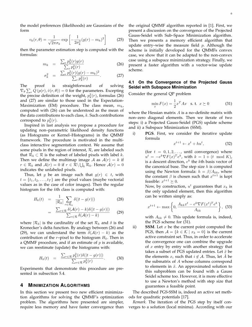
the model preferences (likelihoods) are Gaussians of theform

vk(r, θ) =1√

2πσkexp

[− 1

2σ2k

(g(r)−mk)2]

(25)

then the parameter estimation step is computed with theformulas:

mk =

∑r p

2k(r)g(r)∑x p

2k(r)

(26)

σ2k =

∑r p

2k(r)(g(r)−mk)2∑

r p2k(r)

. (27)

The proof is straightforward of solving∇θ∑r Q (p(r), v(r, θ)) = 0 for the parameters. Excepting

the precise definition of the weight, p2k(r), formulas (26)and (27) are similar to those used in the Expectation-Maximization (EM) procedure. The class mean, mk,computed with (26) can be understood as the mean ofthe data contributions to each class, k. Such contributionscorrespond to p2k(r).

Inspired in last analysis we propose a procedure forupdating non–parametric likelihood density functions(as Histograms or Kernel–Histograms) in the QMMFframework. The procedure is motivated in the multi-class interactive segmentation context. We assume thatsome pixels in the region of interest, R, are labeled suchthat Rk ⊂ R is the subset of labeled pixels with label k.Then we define the multimap image A as A(r) = k ifr ∈ Rk and A(r) = 0 if r ∈ R\⋃kRk. Hence A(r) = 0indicates the unlabeled pixels.

Thus, let g be an image such that g(r) ∈ t, witht = t1, t2, . . . , tT are the pixel values (maybe vectorialvalues as in the case of color images). Then the regularhistogram for the kth class is computed with:

Hk(t) =1

|Rk|∑

r∈Rk

δ(|t− g(r)|) (28)

=

∑r∈R δ(A(r)− k)δ(|t− g(r)|)∑

r∈R δ(A(r)− k)(29)

where |Rk| is the cardinality of the set Rk and δ is theKronecker’s delta function. By analogy between (26) and(29), we can understand the term δ(A(r) − k) as thecontribution of the r–pixel to the histogram Hk. Then ina QMMF procedure, and if an estimate of p is available,we can reestimate (update) the histograms with:

Hk(t) =

∑r∈R p

2k(r)δ(|t− g(r)|)∑r∈R p

2k(r)

. (30)

Experiments that demonstrate this procedure are pre-sented in subsection 5.4.

4 MINIMIZATION ALGORITHMS

In this section we present two new efficient minimiza-tion algorithms for solving the QMMF’s optimizationproblem. The algorithms here presented are simpler,require less memory and have faster convergence than

the original QMMF algorithm reported in [1]. First, wepresent a discussion on the convergence of the ProjectedGauss-Seidel with Sub–Space Minimization algorithm.Then we presents a memory efficient algorithm thatupdate entry–wise the measure field p. Although thescheme is initially developed for the QMMFs convexcase, we show that it can be adapted to the non-convexcase using a subspace minimization strategy. Finally, wepresent a faster algorithm with a vector-wise updatescheme.

4.1 On the Convergence of the Projected GaussSeidel with Subspace Minimization

Consider the general QP problem

minxF (x) =

1

2xTAx s. t. x 0 (31)

where the Hessian matrix A is a no–definite matrix withnon–zero diagonal elements. Then we iterate of twosteps: i) a Projected Gauss-Seidel (PGS) update schemeand ii) a Subspace Minimization (SSM).

i) PGS. First, we consider the iterative updateformula

xt+1 ← xt + hut, (32)

(for t = 0, 1, 2, . . . , until convergence) whereut = −ek∇F (x)T ek, with k = 1 + (t mod K),is a descent direction, ek the kth basis vector ofthe canonical base. The step size h is computedusing the Newton formula: h = β/Akk, wherethe constant β is chosen such that xt+1 is keptfeasible: xt+1 0.Now, by construction, ut guarantees that xk isthe only updated element, then this algorithmcan be written simply as:

xt+1 ← max

0,Akkx

t − ek∇F (xt)T ek

Akk

, (33)

with Akk 6= 0. This update formula is, indeed,the PGS scheme for (31).

ii) SSM. Let x be the current point computed thePGS, then A = k ∈ K | xk = 0 is the currentactive constraint set. Thus, in order to acceleratethe convergence one can combine the upgradeof x entry by entry with another strategy thattakes a subset of PGS updated entries. Let x bethe elements xi such that i 6∈ A. Thus, let A bethe submatrix of A whose columns correspondto elements in x. An approximated solution tothis subproblem can be found with a GaussSeidel scheme too. However, it is more effectiveto use a Newton’s method with step size thatguarantees a feasible point.

The described PGS-SSM is, indeed an active set meth-ods for quadratic potentials [17].

Remark. The iteration of the PGS step by itself con-verges to a solution (local minima). According with our

7

experiments, the SSM step improves significantly theconvergence time.

Note that if the problem (31) includes an equality con-straint of the form Ax = b where the matrix A has linearindependent rows, one can use a variable eliminationtechnique, see Ref. [17], in order to write the originalproblem in form of (31). In our particular case, theconstraint 1T p(r) = 1 (for all r and for a selected class i)can be eliminated by substituting pi(r) = 1−∑k 6=i pk(r)into the energy U(p).

4.2 Memory Limited Gauss Seidel SchemeLet d be a vector field defined as

dk(r)def= − log vk(r)− µ. (34)

Then, if the entropy control µ is chosen such that theenergy (9) is kept convex (dk(r) > 0, ∀k, r) then thecomputation of p consists in solving a linear system. Thisis stated in next proposition.

Proposition 4.1: (Convex QMMF) Let U(p) be the en-ergy function defined in (9) and assume dr 0, then thesolution to

minpU(p) s.t. 1T p(r) = 1, for r ∈ Ω

is a probability measure field: it holds pr 0.Proof: We present an algorithmic proof to this Propo-

sition. The optimal solution satisfies the Karush-Kuhn-Tucker (KKT) conditions:

pk(r)dk(r) + λ∑

s∈Nr

(pk(r)− pk(s))wrs = π(r) (35)

1T p(r) = 1 (36)

where π is the vector of Lagrange’s multipliers. Note thatthe KKT conditions are a symmetric and positive definitelinear system that can be solved with very efficient algo-rithms such as Conjugate Gradient or Multigrid Gauss–Seidel. In particular, a simple Gauss-Seidel (GS) schemeresults from integrating (35) w.r.t. k (i.e. by summingover k) and using (36):

π(r) =1

Kd(r)T p(r). (37)

Thus, from (35):

pk(r) = bk(r) [pk(r) + π(r)] (38)

where we defined:

pk(r)def= λ

∑

s∈Nr

wrspk(s) (39)

andbk(r)

def=

1

dk(r) + λ∑s∈Nr

wrs. (40)

Eqs. (37) and (38) define a two step iterative algorithm.Moreover, if (37) is substituted into (38), we can note thatif an initial p is chosen positive, then the GS scheme (38)will produce a convergent nonnegative sequence.

In addition, the entropy of the solution p can becontrolled by means of the µ parameter that penalizesthe Gini’s (entropy) coefficient. A positive µ reduces theentropy but may result in a negative value of dk(r), see(34), and hence it leads us to a nonconvex QP problem. Inthis case, we can use the projection strategy for enforcingthe non-negativity constraint. Then at each iteration, theprojected p can be computed with

pk(r) = max 0, bk(r)[p(r) + π(r)] . (41)

Algorithm 1 summarizes the PGS procedure for updat-ing a single vector p(r). The complete process repeats thePGS step for all the pixel positions until convergence.

One can see that the GS scheme, here proposed [Eqs.(37) and (38)], is simpler than the originally reported in[1].

Algorithm 1 Simple Projected Gauss Seidel for QMMF.Update procedure for the p(r) vector.

1: Requirei. Let K be the number of classes, λ ≥ 0 the

regularization parameter, v the normalizedlikelihood and w the intra-pixel affinity;

ii. Given dk(r) computed with (34) ;iii. Let r be the current pixel position and p 0;

2: for all k do3: Update π(r) with (37);4: Update pk(r) with (41);5: end for

In order to accelerate the algorithm convergence, wecombine the PGS and the Subspace Minimization strate-gies. First we update p(r) with the PGS scheme byneglecting the nonnegative constraints. Next, at eachpixel, we estimate the active set Ar from the non-positivecoefficients in p(r). Then, we refine the previous solutionby fixing pi(r) = 0 for i ∈ Ar and solving (8) for theremaining pi(r) with i /∈ Ar. If an updated coefficientresults negative, then the active set Ar is updated anda new partial solution is computed. The partial solutionafter few subspace minimizations (we used 2 recursionsin our experiments) is used as starting point for a newPGS iteration. The procedure details are in the Algorithm2. Note that the subspace minimization (line 6) canbe computed with the same algorithm, in a recursiveprocedure.

In Addition, the GS scheme for the binary (two classes)segmentation can be simplified with the elimination ofthe variable p2 (using p2 = 1 − p1). In such a case, theGS update formula is given by

p1(r) =d2(r) + λ

∑s∈Nr

wrsp1(s)

d1(r) + d2(r) + λ∑s∈Nr

wrs. (42)

Finally, we can also use the projection strategy in thenon-convex case. In such a case, the projection needs totake into account both p1(r) and [1− p1(r)]; i.e.,

p1(r)← max0,minp1(r), 1. (43)

8

Algorithm 2 Non–Convex QMMF with subspace mini-mization

1: Initializationi. Let K be the number of classes, λ ≥ 0 the

regularization parameter, v the normalizedlikelihoods and w the intra-pixel affinity;

ii. Compute dk(r) with (34) ;iii. Compute bk(r) with (40) ;v. Initialize p 0; e.g. p = v

2: repeat3: for all r do4: Update p(r) with Algorithm 1;5: Compute an estimate of the active set for p(r):

A = k ∈ K | pk ≤ 0;6: Solve approximatelly (8) for pr fixing pir = 0 for

i ∈ A and p(s) for s 6= r.7: Set p(r) = pr.8: end for9: until convergence

4.3 Vector-wise Gauss Seidel SchemeSince the iterative update formula (38) [and its projectedversion(41)] requires of a reduced amount of memory,its is proper for processing large data, as video ortomographic images (MRI or TC volumes). On the otherhand, we can improve the computational performance(convergence rate) with an extra memory cost if, insteadof updating p(r) component by component, we updatethe entire vector in a single step. First we write the KKTconditions (35) for the full vector p(r):

Drp(r) + λ∑

s∈Nr

(p(r)− p(s))wrs = π(r)1. (44)

Note that the KKT conditions (44) and (36) still are asymmetric and positive definite linear system. Followinga similar algebraic procedure as the one used in section4.2 we have the positive definite and diagonal dominantsystem:

Hrp(r) = pr (45)

with Hr = Dr + Λr − 1dTr , with 1 = 1/K; where wedefine the diagonal matrix Λr

def=(λ∑y∈Nr

wrs

)I and

the kth component of the vector p(r) is computed with(39). Then, the inverse matrix H−1r can efficiently becomputed with the Sherman-Morrison formula. Thus

H−1r = Br +Br1d(r)TBr

1− 1TBrd(r)(46)

where we define the positive diagonal matrix Br =diag[ b(r)] with the elements of b(r) computed with (40).Hence, we note that

1TBrd(r) =1

K

∑

k∈K

dk(r)

bk(r)< 1

because λ > 0 and then dk(r)bk(r)

= dk(r)

dk(r)+λ∑

spk(s)

< 1.

Thus H−1 0 (has non negative elements) is positive

definite (it does not have rows equal to zero). Conse-quently, the iteration of

p(r) = H−1r p(r),∀r (47)

keeps p 0 if the initial p is chosen positive.Now, we give an extra step for simplify the update

formula. First, we note that Br1 = b(r)/K. Second, wedefine pre–computable vector (independent of p):

d(r)T =1

K − b(r)T d(r)d(r)TBr. (48)

Next, we define the product:

π(r) = d(r)T p(r). (49)

Finally, the kth component of p(r) in (47) can be com-puted the simple formula:

pk(r) = bk(r) [pk(r) + π(r)] . (50)

Note the similarity with (39), the difference is the for-mula for computing π; compare (37) with (49). Thecomplete procedure is summarized in Algorithm 3.

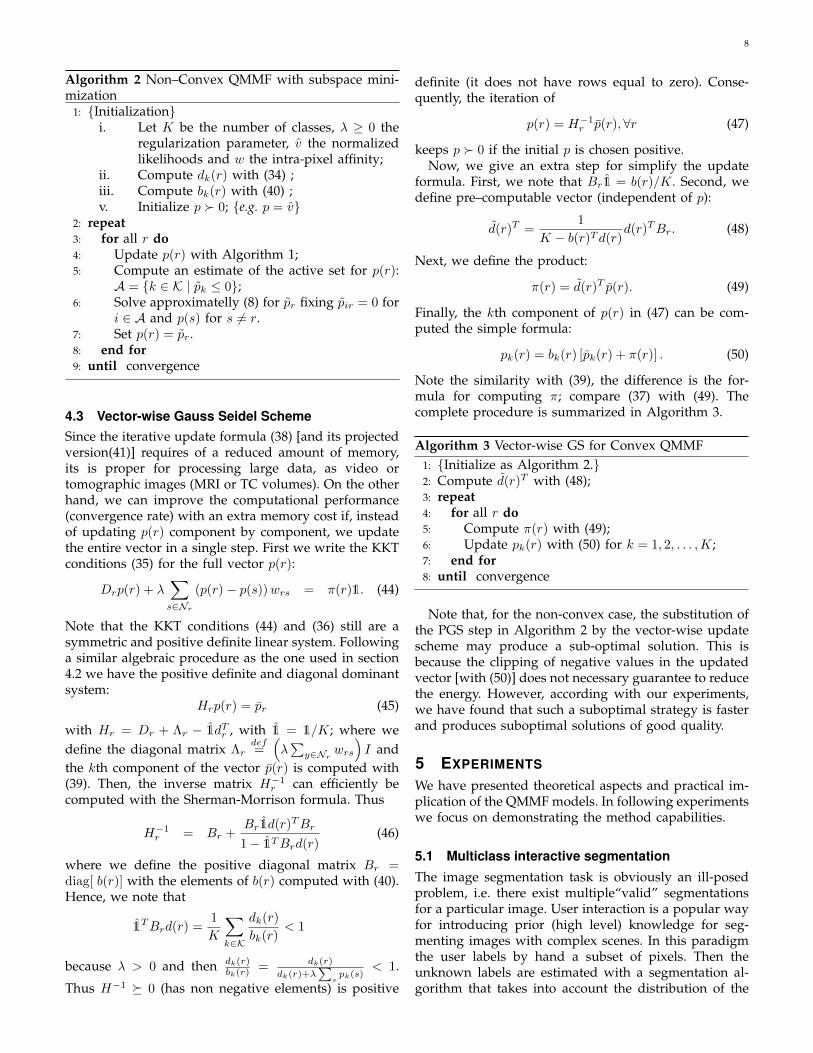
Algorithm 3 Vector-wise GS for Convex QMMF1: Initialize as Algorithm 2.2: Compute d(r)T with (48);3: repeat4: for all r do5: Compute π(r) with (49);6: Update pk(r) with (50) for k = 1, 2, . . . ,K;7: end for8: until convergence

Note that, for the non-convex case, the substitution ofthe PGS step in Algorithm 2 by the vector-wise updatescheme may produce a sub-optimal solution. This isbecause the clipping of negative values in the updatedvector [with (50)] does not necessary guarantee to reducethe energy. However, according with our experiments,we have found that such a suboptimal strategy is fasterand produces suboptimal solutions of good quality.

5 EXPERIMENTS

We have presented theoretical aspects and practical im-plication of the QMMF models. In following experimentswe focus on demonstrating the method capabilities.

5.1 Multiclass interactive segmentationThe image segmentation task is obviously an ill-posedproblem, i.e. there exist multiple“valid” segmentationsfor a particular image. User interaction is a popular wayfor introducing prior (high level) knowledge for seg-menting images with complex scenes. In this paradigmthe user labels by hand a subset of pixels. Then theunknown labels are estimated with a segmentation al-gorithm that takes into account the distribution of the

99

Fig. 2. Interactive multi–class segmentations.

labelled pixels and the smoothness of the spatial seg-mentation. Interactive segmentation is an approach thatallows us to develop general purpose tools. To illustratethis, we can see three possible segmentations of theimage in Fig. 1. The first column shows scribbles givenby the user and the second column the correspondingsegmentations computed with the method here pre-sented. The rows correspond to segmentation by color,semantical objects (house, vegetation, fence, etc.) andplanar regions; respectively.

The likelihood functions are estimated using his-tograms, as is described in section 3.4.3. Such histogramsare computed using (29). Thus the normalized his-tograms are computed with hki = Hk(ti)/

∑lHk(ti) and

the likelihood of the pixel r to belong to a given class k(likelihood function, LF) is computed with:

LFki =hki + ε

∑j(hji + ε)

, ∀k; (51)

with ε = 1 × 10−8, a small constant. The ε scalar intro-duces an uniform distribution that avoids a possible di-vision by zero and guarantee positive likelihoods. Thusthe likelihood of an observed pixel value is computedwith vk(r) = LFki such that i = arg minj ‖g(r)− tj‖2.

In this experiments, we assume that the user’s labelsare correct; then, in the data term in (9), the sum overall the pixels in the region of interest, r ∈ R, isreplaced by the sum over the unlabeled pixels; i.e., forr ∈ R : A(r) = 0. Alternatively, the sum for all pixelssupposes may be incorrectly hand labelled pixels.

Figure 2 shows multi–class interactive segmentationscomputed with the proposed algorithm implementedin Matlab (in .m and .mex files). Moreover, we useTg(r) = v(r) in (21).

5.2 Color/Texture based Interactive Segmentation

Texture is evidently an important clue to be considerin image segmentations. As color Likelihood Functions(LFs), feature–texture LFs can be learned from user’sscribbles and can be represented with non-parametric(or parametric) models. In the case of color, it seems

Fig. 3. Color and Texture based interactive segmenta-tions: user’s scribbles (first column), color based segmen-tation(second column) and color/texture based segmen-tation (third column)

TABLE 2Cross-validation results: Parameters, Akaike information

criterion, training and testing error.

Algorithm Params. AIC Training TestingGraph Cut λ, γ 8.58 6.82% 6.93%Rand. Walk. λ, γ 6.50 5.46% 5.50%GMMF λ, γ 6.49 5.46% 5.49%QMMF λ, γ 6.04 5.02% 5.15%QMMF+EC λ, γ, µ 3.58 3.13% 3.13%

natural that the joint LFs are represented by 3D his-tograms (corresponding to the 3D color representation).Since texture features vector are in general representedin dimensions higher than 3, one can use a dimensionreduction technique (as PCA) in order to find a represen-tation with linearly independent coordinates and thenuse low–dimensional histograms. Different to the PCAapproach, in section 3.4.2 we proposed method that findsthe most significant features for segmenting a particularimage: it takes advantage of the information codifiedin user’s scribbles. In the experiment, we use the fivemost significant features (largest α) and 3D histogramsas Likelihood Function for each cosine transform rgb–coefficient. According to our experiments, the use of thewhole feature vector produces similar results, but itsis more efficient in memory usage to use just the fivemore significant DCT coefficients. The Fig. 3 presentscomparative results of a color–based segmentation andthe proposed color/texture based segmentation.

5.3 Quantitative Comparisson: Image Binary Inter-active SegmentationNext, we summarize our results of a quantitative studyon the performance of the segmentation algorithms:the proposed Binary variant of QMMF, the max–flow




∑lHk(ti) and


LFki =hki + ε

∑j(hji + ε)

, ∀k; (51)




5.2 Color/Texture based Interactive SegmentationTexture is evidently an important clue to be considerin image segmentations. As color Likelihood Functions(LFs), feature–texture LFs can be learned from user’sscribbles and can be represented with non-parametric(or parametric) models. In the case of color, it seemsnatural that the joint LFs are represented by 3D his-tograms (corresponding to the 3D color representation).

9




∑lHk(ti) and


LFki =hki + ε

∑j(hji + ε)

, ∀k; (51)




5.2 Color/Texture based Interactive Segmentation

Texture is evidently an important clue to be considerin image segmentations. As color Likelihood Functions(LFs), feature–texture LFs can be learned from user’sscribbles and can be represented with non-parametric(or parametric) models. In the case of color, it seems





natural that the joint LFs are represented by 3D his-tograms (corresponding to the 3D color representation).Since texture features vector are in general representedin dimensions higher than 3, one can use a dimensionreduction technique (as PCA) in order to find a represen-tation with linearly independent coordinates and thenuse low–dimensional histograms. Different to the PCAapproach, in section 3.4.2 we proposed method that findsthe most significant features for segmenting a particularimage: it takes advantage of the information codifiedin user’s scribbles. In the experiment, we use the fivemost significant features (largest α) and 3D histogramsas Likelihood Function for each cosine transform rgb–coefficient. According to our experiments, the use of thewhole feature vector produces similar results, but itsis more efficient in memory usage to use just the fivemore significant DCT coefficients. The Fig. 3 presentscomparative results of a color–based segmentation andthe proposed color/texture based segmentation.

5.3 Quantitative Comparisson: Image Binary Inter-active SegmentationNext, we summarize our results of a quantitative studyon the performance of the segmentation algorithms:the proposed Binary variant of QMMF, the max–flow





Since texture features vector are in general representedin dimensions higher than 3, one can use a dimensionreduction technique (as PCA) in order to find a represen-tation with linearly independent coordinates and thenuse low–dimensional histograms. Different to the PCAapproach, in section 3.4.2 we proposed method that findsthe most significant features for segmenting a particularimage: it takes advantage of the information codifiedin user’s scribbles. In the experiment, we use the fivemost significant features (largest α) and 3D histogramsas Likelihood Function for each cosine transform rgb–coefficient. According to our experiments, the use of thewhole feature vector produces similar results, but itsis more efficient in memory usage to use just the fivemore significant DCT coefficients. The Fig. 3 presentscomparative results of a color–based segmentation andthe proposed color/texture based segmentation.

5.3 Quantitative Comparisson: Image Binary Inter-active Segmentation

Next, we summarize our results of a quantitative studyon the performance of the segmentation algorithms:the proposed Binary variant of QMMF, the max–flow(min–graph–cut), GMMF and Random Walker (RW).The reader can find more details about this study in

10

TABLE 3Adjusted parameters for the results in table 2.

GC RW GMMF QMMF EC–QMMF

λ(×103) 0.128 2700 2100 4.7 230γ(×106) 27 3.7 3.7 9.14 5700µ(×103) — — — — −570

10



λ(×103) 0.128 2700 2100 4.7 230γ(×106) 27 3.7 3.7 9.14 5700µ(×103) — — — — −570

(a) Original (b) Trimap (c) GraphCut (d) QMMF+EC

Fig. 4. Segmentation example from the Lasso’s data set.

(min–graph–cut), GMMF and Random Walker (RW).The reader can find more details about this study inour technical report [19]. We used our implementationfor the GMMF and RW algorithms, and the authors’implementation of the max–flow/graph–cut algorithmdescribed in [28] for minimizing the energy:

U(p) =∑

r:A(r)=0

b(r)v1(r) + [1− b(r)]v2(r)

+λ

2

∑

s∈Nr

wrs[1− δ(b(r)− b(s)]

(52)

with b(r) ∈ 0, 1.The task is to segment color images into background

and foreground allowing interactive data labeling. Thegeneralization capabilities of the methods are comparedwith a cross-validation procedure [25]. The comparisonwas conducted on the Lasso benchmark database [7]; aset of 50 images available online [29]. Such a databasecontains a natural image set with their correspondingtrimaps and the ground truth segmentations. Actually, aLasso trimap is an image of class labels: no–process mask(M = L\R), background, foreground and unknown;where no error is assumed in the initial labelled pixels.First column in Fig. 4 shows an image from the Lassodatabase and second column the corresponding trimap;the gray scale corresponds with the above class enumer-ation. In this case, the region to process is labeled as“unknown” and the boundary conditions are imposedby the foreground and background labeled regions.

We opted to compute the weights using the standardformula (21) (i.e. Tg(r) = g(r) in (21) ). In order tofocus our comparison on the data term of the differentalgorithms: QMMF, GC, GMMF and RW. In this task,empirical likelihoods are computed from the histogramof the hand labeled pixels [8]. Figure 5 shows examplesof segmented objects from images in the Lasso database.One set corresponds to the results of the GraphCut (GC)considered the estate of the art and the second group tothe EC-QMMF.

The hyper parameters (λ, µ, γ) were trained by mini-mizing the mean of the segmentation error in the image

(a) GraphCut

(b) EC-QMMF

Fig. 5. Segmented objects with GC (upper group) andEC–QMMF (lower group) algorithms.

set by using the Nelder and Mead simplex descent [30].We implement a cross–validation procedure followingthe recommendation in Ref. [25] and split the data setinto 5 set s, 10 images per set. Figure 4 shows an exampleof the segmented images. Table 2 shows summarizesthe Akaike Information Criterion (AIC) [25] and thetraining and testing error. The AIC was computed for theoptimized (trained) parameters with the 50 image in thedatabase. Note that the AIC is consistent with the cross-validation results: the order of the method performanceis preserved. Moreover the QMMF algorithm has thebest performance in the group. Table 3 shows the learntparameters for the evaluated methods. In the case of theEC-QMMF, the computational time was about 0.2 sec.for the Lasso images. This automatic learning parameterprocess confirms that GMMF and RW, as close variants,have similar performance [19]. However, it produces twounexpected results:

i. Our GC based segmentation improves significantlythe reported results in [7]. Indeed, our basic GCformulation of the method in [8] overcomes, signif-icantly, the reported results with Likelihood Func-tions based on Gaussian Mixtures [7].

ii. The learnt parameter µ (EC-QMMF) promotes largeentropy. In our opinion, there are three reasons forsuch result: the Lasso dataset have a narrow bandof unknown pixels; the trimaps are correct, so thatthe class models (histograms) are reliable; and thehand–segmentations (ground truth) favor smooth


our technical report [19]. We used our implementationfor the GMMF and RW algorithms, and the authors’implementation of the max–flow/graph–cut algorithmdescribed in [28] for minimizing the energy:

U(p) =∑

r:A(r)=0

b(r)v1(r) + [1− b(r)]v2(r)

+λ

2

∑

s∈Nr


(52)




The hyper parameters (λ, µ, γ) were trained by mini-mizing the mean of the segmentation error in the imageset by using the Nelder and Mead simplex descent [30].We implement a cross–validation procedure followingthe recommendation in Ref. [25] and split the data set

10



λ(×103) 0.128 2700 2100 4.7 230γ(×106) 27 3.7 3.7 9.14 5700µ(×103) — — — — −570

(a) Original (b) Trimap (c) GraphCut (d) QMMF+EC


(min–graph–cut), GMMF and Random Walker (RW).The reader can find more details about this study inour technical report [19]. We used our implementationfor the GMMF and RW algorithms, and the authors’implementation of the max–flow/graph–cut algorithmdescribed in [28] for minimizing the energy:

U(p) =∑

r:A(r)=0

b(r)v1(r) + [1− b(r)]v2(r)

+λ

2

∑

s∈Nr


(52)




The hyper parameters (λ, µ, γ) were trained by mini-mizing the mean of the segmentation error in the image

(a) GraphCut

(b) EC-QMMF


set by using the Nelder and Mead simplex descent [30].We implement a cross–validation procedure followingthe recommendation in Ref. [25] and split the data setinto 5 set s, 10 images per set. Figure 4 shows an exampleof the segmented images. Table 2 shows summarizesthe Akaike Information Criterion (AIC) [25] and thetraining and testing error. The AIC was computed for theoptimized (trained) parameters with the 50 image in thedatabase. Note that the AIC is consistent with the cross-validation results: the order of the method performanceis preserved. Moreover the QMMF algorithm has thebest performance in the group. Table 3 shows the learntparameters for the evaluated methods. In the case of theEC-QMMF, the computational time was about 0.2 sec.for the Lasso images. This automatic learning parameterprocess confirms that GMMF and RW, as close variants,have similar performance [19]. However, it produces twounexpected results:


ii. The learnt parameter µ (EC-QMMF) promotes largeentropy. In our opinion, there are three reasons forsuch result: the Lasso dataset have a narrow bandof unknown pixels; the trimaps are correct, so thatthe class models (histograms) are reliable; and thehand–segmentations (ground truth) favor smooth


into 5 set s, 10 images per set. Figure 4 shows an exampleof the segmented images. Table 2 shows summarizesthe Akaike Information Criterion (AIC) [25] and thetraining and testing error. The AIC was computed for theoptimized (trained) parameters with the 50 image in thedatabase. Note that the AIC is consistent with the cross-validation results: the order of the method performanceis preserved. Moreover the QMMF algorithm has thebest performance in the group. Table 3 shows the learntparameters for the evaluated methods. In the case of theEC-QMMF, the computational time was about 0.2 sec.for the Lasso images. This automatic learning parameterprocess confirms that GMMF and RW, as close variants,have similar performance [19]. However, it produces twounexpected results:


ii. The learnt parameter µ (EC-QMMF) promotes largeentropy. In our opinion, there are three reasons forsuch result: the Lasso dataset have a narrow bandof unknown pixels; the trimaps are correct, so thatthe class models (histograms) are reliable; and thehand–segmentations (ground truth) favor smoothboundaries.

This results remark the importance of the presentedvariational derivation for the QMMFs that does notconstraint the entropy to be small (Section 3). However,

1111

Fig. 6. Simultaneous segmentation and parameter esti-mation. From left to right: original image (200×200 pixels),noisy image (σ = 1.8), segmentation with µ = 0 and withµ = 20.

0 0.5 1 1.5 2 2.5 3 3.5 40

20

40

60

80

100

Std. dev

Percent of success

QMMFEC−QMMF

Fig. 7. Simultaneous segmentation and parameter esti-mation. Results on 100 Montecarlo experiments: numberof correct successful detected parameters versus theSNR, see text.

boundaries.This results remark the importance of the presented

variational derivation for the QMMFs that does notconstraint the entropy to be small (Section 3). However,next experiment demonstrates that for the simultaneousestimation of the segmentation and the model parame-ters the uncertainty in the solution (entropy) need to becontrolled and small.

5.4 Model parameter estimation

The entropy control allows us to adapt the algorithmfor different tasks. For example, lower entropy producesbetter results for the task of simultaneously estimationof segmentation and model parameters, see Section 3.4.3.Next, we describe an experiment that demonstrate lastclaim. The test image is the one shown in Fig. 6. Theimage has 8 regions and the colors correspond to thevertices of the rgb color–space cube. Then, such colorsare the model parameter mk, for k = 1, 2, . . . , 8. Thecolors were normalized; i.e. m1 = [0, 0, 0] (black) andm8 = [1, 1, 1] (white). Then the image was corruptedwith Gaussian noise with different standard deviation(SNR) levels σn. For each noise level, 100 Montecarloexperiments were performed. Each experiment consistedof three stages: a) to generate a random noisy image(with Gaussian noise), b) to initialize 12 means (1.5 thenumber of true model number) and c) to estimate theoriginal image colors (parameters) and the segmentationwith QMMF algorithm. The last step was implemented

Fig. 8. Iterative estimation of empirical likelihood func-tions by histograms of p2–weighted data. Binary segmen-tation: initial scribbles, first iteration and second iteration;respective columns.

with eight iteration of the Segmentation/Parameter-estimation steps. We marked an experiment as “success”if at least a mean (of the 12) converge to each regionMk = z ∈ RK | ‖z −mk‖1 < 1, ∀k. Figure 6 showsan instance of the random images (with σ = 1.8); itsfailed segmentation with the QMMF with µ = 0 (no-entropy control) and its successful segmentation withEC-QMMF, µ = 20. The over–segmentation (in theEC-QMMF segmentation) can be reduced by groupingregions, but such a step is beyond the scope of thiswork. Figure 7 summarize the Montecarlo experimentresults. The λ parameter was tuned with the thumbrule: λ = 10(1 + floor(σ)); then µ = 0 for the non-entropy control case (QMMF) and µ = λ for EC-QMMF.As the QMMF (µ = 0), our implementations based onGauss Markov Measure Fields (GMMF, an early variantof Random Walker [6]) collapsed to a single model [4].This limitation of the GMMF model is discussed in [31],see also [19].

Finally, we demonstrate the generalization of theQMMFs for the joint task of segmentation and non-parametric Likelihood Functions (LF) estimation,based on histogram techniques. The segmentationis computed after two iteration of the stagesSegmentation/Parameter-estimation. First at all, theinitial histograms are computed according (30) usingp = v. Then, the QMMF–segmentation is computed.After, the histograms areupdated using (30). Finally,the QMMF–segmentation is recomputed. Different fromSection 5.1, in this case the region of interest is thecomplete image; i.e., the labels of the user markedpixels (multimap) are also estimated. The process isillustrated in Fig. 8: the erroneous segmentation afterthe first iteration is product of inaccurate scribbles andthus an inaccurate initial LF. The segmentation, aftertwo iterations, demonstrate the ability of the QMMFsfor estimating nonparametric class distributions.


0 0.5 1 1.5 2 2.5 3 3.5 40

20

40

60

80

100

Std. dev

Percent of success

QMMFEC−QMMF


next experiment demonstrates that for the simultaneousestimation of the segmentation and the model parame-ters the uncertainty in the solution (entropy) need to becontrolled and small.

5.4 Model parameter estimationThe entropy control allows us to adapt the algorithmfor different tasks. For example, lower entropy producesbetter results for the task of simultaneously estimationof segmentation and model parameters, see Section 3.4.3.Next, we describe an experiment that demonstrate lastclaim. The test image is the one shown in Fig. 6. Theimage has 8 regions and the colors correspond to thevertices of the rgb color–space cube. Then, such colorsare the model parameter mk, for k = 1, 2, . . . , 8. Thecolors were normalized; i.e. m1 = [0, 0, 0] (black) andm8 = [1, 1, 1] (white). Then the image was corruptedwith Gaussian noise with different standard deviation(SNR) levels σn. For each noise level, 100 Montecarloexperiments were performed. Each experiment consistedof three stages: a) to generate a random noisy image(with Gaussian noise), b) to initialize 12 means (1.5 thenumber of true model number) and c) to estimate theoriginal image colors (parameters) and the segmentationwith QMMF algorithm. The last step was implementedwith eight iteration of the Segmentation/Parameter-estimation steps. We marked an experiment as “success”if at least a mean (of the 12) converge to each regionMk = z ∈ RK | ‖z −mk‖1 < 1, ∀k. Figure 6 showsan instance of the random images (with σ = 1.8); its

11


0 0.5 1 1.5 2 2.5 3 3.5 40

20

40

60

80

100

Std. dev

Percent of success

QMMFEC−QMMF


boundaries.This results remark the importance of the presented

variational derivation for the QMMFs that does notconstraint the entropy to be small (Section 3). However,next experiment demonstrates that for the simultaneousestimation of the segmentation and the model parame-ters the uncertainty in the solution (entropy) need to becontrolled and small.

5.4 Model parameter estimation

The entropy control allows us to adapt the algorithmfor different tasks. For example, lower entropy producesbetter results for the task of simultaneously estimationof segmentation and model parameters, see Section 3.4.3.Next, we describe an experiment that demonstrate lastclaim. The test image is the one shown in Fig. 6. Theimage has 8 regions and the colors correspond to thevertices of the rgb color–space cube. Then, such colorsare the model parameter mk, for k = 1, 2, . . . , 8. Thecolors were normalized; i.e. m1 = [0, 0, 0] (black) andm8 = [1, 1, 1] (white). Then the image was corruptedwith Gaussian noise with different standard deviation(SNR) levels σn. For each noise level, 100 Montecarloexperiments were performed. Each experiment consistedof three stages: a) to generate a random noisy image(with Gaussian noise), b) to initialize 12 means (1.5 thenumber of true model number) and c) to estimate theoriginal image colors (parameters) and the segmentationwith QMMF algorithm. The last step was implemented


with eight iteration of the Segmentation/Parameter-estimation steps. We marked an experiment as “success”if at least a mean (of the 12) converge to each regionMk = z ∈ RK | ‖z −mk‖1 < 1, ∀k. Figure 6 showsan instance of the random images (with σ = 1.8); itsfailed segmentation with the QMMF with µ = 0 (no-entropy control) and its successful segmentation withEC-QMMF, µ = 20. The over–segmentation (in theEC-QMMF segmentation) can be reduced by groupingregions, but such a step is beyond the scope of thiswork. Figure 7 summarize the Montecarlo experimentresults. The λ parameter was tuned with the thumbrule: λ = 10(1 + floor(σ)); then µ = 0 for the non-entropy control case (QMMF) and µ = λ for EC-QMMF.As the QMMF (µ = 0), our implementations based onGauss Markov Measure Fields (GMMF, an early variantof Random Walker [6]) collapsed to a single model [4].This limitation of the GMMF model is discussed in [31],see also [19].

Finally, we demonstrate the generalization of theQMMFs for the joint task of segmentation and non-parametric Likelihood Functions (LF) estimation,based on histogram techniques. The segmentationis computed after two iteration of the stagesSegmentation/Parameter-estimation. First at all, theinitial histograms are computed according (30) usingp = v. Then, the QMMF–segmentation is computed.After, the histograms areupdated using (30). Finally,the QMMF–segmentation is recomputed. Different fromSection 5.1, in this case the region of interest is thecomplete image; i.e., the labels of the user markedpixels (multimap) are also estimated. The process isillustrated in Fig. 8: the erroneous segmentation afterthe first iteration is product of inaccurate scribbles andthus an inaccurate initial LF. The segmentation, aftertwo iterations, demonstrate the ability of the QMMFsfor estimating nonparametric class distributions.


failed segmentation with the QMMF with µ = 0 (no-entropy control) and its successful segmentation withEC-QMMF, µ = 20. The over–segmentation (in theEC-QMMF segmentation) can be reduced by groupingregions, but such a step is beyond the scope of thiswork. Figure 7 summarize the Montecarlo experimentresults. The λ parameter was tuned with the thumbrule: λ = 10(1 + floor(σ)); then µ = 0 for the non-entropy control case (QMMF) and µ = λ for EC-QMMF.As the QMMF (µ = 0), our implementations based onGauss Markov Measure Fields (GMMF, an early variantof Random Walker [6]) collapsed to a single model [4].This limitation of the GMMF model is discussed in [31],see also [19].

Finally, we demonstrate the generalization of theQMMFs for the joint task of segmentation and non-parametric Likelihood Functions (LF) estimation,based on histogram techniques. The segmentationis computed after two iteration of the stagesSegmentation/Parameter-estimation. First at all, theinitial histograms are computed according (30) usingp = v. Then, the QMMF–segmentation is computed.After, the histograms are updated using (30). Finally,the QMMF–segmentation is recomputed. Different fromSection 5.1, in this case the region of interest is thecomplete image; i.e., the labels of the user markedpixels (multimap) are also estimated. The process isillustrated in Fig. 8: the erroneous segmentation afterthe first iteration is product of inaccurate scribbles andthus an inaccurate initial LF. The segmentation, aftertwo iterations, demonstrate the ability of the QMMFsfor estimating nonparametric class distributions.

6 CONCLUSIONS AND DISCUSSION

Image segmentation consists in partitioning an imageinto regions with similar features of interest (color, tex-ture, motion, depth, etc.) or semantical properties (kind

12

tissue in medical images, objects in a scene, roads inaerial images, etc.). The image regions provides a com-pact representation that allows one to make inferenceon the image properties. Therefore image segmentationis an active research topic in computer vision and imageanalysis. It is a core process in many practical applica-tions. In this work, we studied theoretical properties,proposed new optimization algorithms and presentedpractical extensions to a recent image segmentationmodel.

We presented a derivation of the QMMF model in-dependent of the minimal entropy constraint. Therefore,based on prior knowledge, we can control the amountof entropy increment, or decrement, in the computedprobability measures. We demonstrated that the QMMFmodels are general and flexible to be used with di-verse Likelihood Functions. As demonstration of such ageneralization, we presented experiments with iterativeestimation of likelihood functions based on histogramtechniques. We proposed robust likelihoods that improvethe method performance for segmenting textured re-gions.

Our contributions in this work are mainly a more gen-eral derivation of the QMMF models and more efficientoptimization algorithms. Along the paper we present aseries of experiments for demonstrating our proposals.Additionally, we present an experimental comparisonwith respect algorithms of the state of the art. Weselected the task of binary interactive segmentation forconducting our comparison, first because it demonstratesthe use of the entropy control in the case of genericlikelihood functions. Second, a benchmark database isonline available, and finally our hyper–parameter train-ing scheme demonstrates to be objective by, significantly,improving the previously reported results with a graphcut based method.

APPENDIX ADefinition (Stieltjes matrices [32]). A K × K Stieltjesmatrix A = (aij) with i, j = 1, 2, . . . ,K satisfies: it issymmetric and positive definite; it has positive diago-nal elements, aii > 0; it has nonpositive off-diagonalelements, aij ≤ 0, i 6= j; and its inverse B = (bij) isnonnegative, bij > 0,∀i, j = 1, 2, . . . ,K.

Proof of Proposition 3.2: The KKT conditions of (15)are

Ax− π1 = 0 (53)1Tx− 1 = 0, (54)

where π is the Lagrange’s multiplier. Then from (53):x = πA−11. Substituting this result in (54), we haveπ1TA−11 = 1, thus π = 1/(1TA−11). We conclude thatx 0, since A is Stieltjes matrix, A−1 is positive definiteand non-negative. Thus, 1TA−11 > 0 (sum over all theelements) and A−11 0 (sum over rows). Note that A−1

has not rows equal zero.

Proof of Proposition 3.3: The KKT conditions of (17)are: d − π1 = ξ,1Tx − 1 = 0, xT ξ = 0, and x, ξ 0;where dk

def= − log yk, π is the Lagrange’s multiplier of

the equality constraint and ξ is the vector of Lagrange’smultiplier of the nonnegativity constraints. Then, by theFundamental Theorem of the Linear programing [17] itcan be seen that the KKTs are fullfil with: x = ek∗ withk∗ = argmin

kdk, π = dk∗ and ξ given by the first KKT.

REFERENCES

[1] M. Rivera, O. Ocegueda, and J. L. Marroquin, “Entropy-controlledquadratic Markov measure field models for efficient image seg-mentation,” IEEE Trans. Image Processing, vol. 8, no. 12, pp. 3047–3057, Dec. 2007.

[2] S. Z. Li, Markov Random Field Modeling in Image Analysis. Springer-Verlag, Tokyo, 2001.

[3] S. Geman and D. Geman, “Stochastic relaxation, Gibbs distribu-tion and the Bayesian restoration of images,” IEEE Trans. PatternAnal. Machine Intell., vol. 6, no. 6, pp. 721–741, 1984.

[4] J. L. Marroquin, F. Velazco, M. Rivera, and M. Nakamura, “Prob-abilistic solution of ill–posed problems in computational vision,”IEEE Trans. Pattern Anal. Machine Intell., vol. 23, pp. 337–348, 2001.

[5] V. Kolmogorov and R. Zabih, “What energy functions can beminimized via graph cuts,” in European Conference on ComputerVision (ECCV02)., 2002.

[6] L. Grady, “Random walks for image segmentation,” IEEE Trans.Pattern Anal. Mach. Intell., vol. 28, no. 11, pp. 1768–1783, 2006.

[7] A. Blake, C. Rother, M. Brown, P. Perez, and P. Torr, “Interactiveimage segmentation using an adaptive GMMRF model,” in ECCV,vol. 1, ser. LNCS 3021, Springer Berlin / Heidelberg, 2004, pp.414–427.

[8] Y. Boykov and M.-P. Jolly, “Interactive graph cut for optimalboundary & region segmentation of objects in N–D images,” inICIP (1), 2001, pp. 105–112.

[9] Y. Boykov, O. Veksler, and R. Zabih, “Fast approximate energyminimization via graph cuts,” IEEE Trans. Pattern Anal. MachineIntell., vol. 23, no. 11, pp. 1222–1239, 2001.

[10] V. Kolmogorov, A. Criminisi, A. Blake, G. Cross, and C. Rother,“Probabilistic fusion of stereo with color and contrast for bi-layersegmentation,” IEEE Trans. Pattern Anal. Mach. Intell., vol. 28,no. 9, pp. 1480–1492, 2006.

[11] C. Rother, V. Kolmogorov, and A. Blake, “Interactive foregroundextraction using iterated graph cuts,” in ACM Transactions onGraphics, no. 23 (3), 2004, pp. 309–314.

[12] C. Olsson, A. P. Eriksson, and F. Kahl, “Improved spectral re-laxation methods for binary quadratic optimization problems,”Computer Vision and Image Understanding, vol. 112, pp. 30–38, 2008.

[13] N. Komodakis, G. Tziritas, and N. Paragios, “Performance vscomputational efficiency for optimizing single and dynamicMRFs: Setting the state of the art with primal–dual strategies,”Computer Vision and Image Understanding, vol. 112, pp. 14–29, 2008.

[14] P. Kohli and P. H. S. Torr, “Measuring uncertainty in graph cutsolutions,” Computer Vision and Image Understanding, vol. 112, pp.30–38, 2008.

[15] M. Rivera, O. Ocegueda, and J. L. Marroquin, “Entropy controlledGauss-Markov random measure fields for early vision,” in in Proc.VLSM, vol. 1 LNCS 3752, Springer Berlin / Heidelberg, 2005, pp.137–148.

[16] A. Levin, A. Rav-Acha, and D. Lischinski, “Spectral matting,”IEEE Trans. Pattern Anal. Mach. Intell., vol. 30, no. 10, pp. 1–14,2008.

[17] J. Nocedal and S. J. Wright, Numerical Optimization. Springer Seriesin Operation Research, 2000.

[18] M. Rivera and P. P. Mayorga, “Quadratic markovian probabilityfields for image binary segmentation,” in in Proc. ICCV, WorkshopICV 07, 2007, pp. 1–8.

[19] ——, “Comparative study on quadratic Markovian probabilityfields for image binary segmentation,” CIMAT A.C., Mexico, Tech.Rep. 10.12.2007, I-07-15 (CC), December 2007.

[20] M. Rivera, O. Dalmau, and J. Tago, “Image segmentation by con-vex quadratic programming,” in Int. Conf. on Pattern Recognition(ICPR08), 2008.

13

[21] O. Dalmau and M. Rivera, “A general bayesian markov randomfield model for probabilistic image segmentation,” in in Procc. Int.Workshop Combinatorial Image Analysis (IWCIA), ser. LNCS 5852,Springer Berlin / Heidelberg, 2009, pp. 149–161.

[22] M. Black and A. Rangarajan, “On the unification of line processes,outlier rejection, and robust statistics with applications in earlyvision,” Int’l J. Computer Vision, vol. 19, no. 1, pp. 57–92, 1996.

[23] B. D. Sharma and R. Autar, “Relative information functions andtheir type (alpha, beta) generalizations,” Metrika, vol. 21, no. 1,pp. 41–50, 1974.

[24] I. Taneja and H. C. Gupta, “On generalized measures of relativeinformation and inaccuracy,” Aplikace Matematiky, vol. 23, pp. 317–333, 1978.

[25] T. Hastie, R. Tibshirani, and J. Friedman, The elements of statisticallearning, Springer, 2001.

[26] D. F. Kerridge, “Inaccuracy and inference,” J. Royal Stat. Soc, Ser.B, vol. 23, no. 1, pp. 184–194, 1961.

[27] M. Rivera, O. Dalmau, and W. Mio, “Spatial sampling for imagessegmentation,” in to appear in International Symposium on Computerand Information Sciences (ISCIS), 2010.

[28] Y. Boykov and V. Kolmogorov, “An experimental comparison ofmin-cut/max-flow algorithms for energy minimization in vision,”Int’l J. Computer Vision, vol. 70, no. 2, pp. 109–131, 2006.

[29] http://research.microsoft.com/vision/cambridge/i3l/segmentation/GrabCut.htm.

[30] J. A. Nelder and R. Mead, “A simplex method for functionminimization,” Comput. J., vol. 7, pp. 308–313, 1965.

[31] J. L. Marroquin, B. C. Vemuri, S. Botello, F. Calderon, andA. Fernandez-Bouzas, “An accurate and efficient Bayesianmethod for automatic segmentation of brain MRI,” IEEE Trans.Medical Imaging, vol. 21, pp. 934–945, 2002.

[32] R. S. Varga, Matrix Iterative Analysis, 2nd ed. Springer Series inComputational Mathematics, 2000, vol. 27.

REFERENCES[1] H. Kopka and P.W. Daly, A Guide to LATEX, third ed. Harlow, U.K.:

Addison-Wesley, 1999.

Mariano Rivera received the B.E. degree inelectronics from the Durango Institute of Tech-nology, Mexico, in 1989, the M.Sc. degree inelectronics from the Chihuahua Institute of Tech-nology,Mexico, in 1993, and the D.Sc. degreein optics from the Center for Research in Op-tics (CIO), Leon, Mexico, in 1997. Since 1997,he has been with the Computer Science De-partment, Center for Research in Mathematics(CIMAT), Guanajuato, Mexico. His current inter-ests include computer vision, image processing,

machine learning, and optimization. His research is summarized in morethan 70 papers in scientific journals and conference proceedings. Dr.Rivera is Fellow of the National Researcher System (SNI) of the MexicanGovernment.

Oscar Dalmau received his BScEd in Math-ematics at ISP Manzanillo Cuba in 1989, hisM.Sc. degree in Computer Science and Indus-trial Mathematics at the Center of Research inMathematics (CIMAT) Mexico in 2004 and hisPh.D. degree in Computer Science at CIMATMexico in 2010. He works at the Center forResearch in Mathematics (CIMAT), Monterrey,Nuevo Leon, Mexico. His research interests liein the areas of machine learning, optimization,and image processing and computer vision.

variational viewpoint of the quadratic markov measure field models

Documents