Variational Calculationsfor Resonance Oscillationsof Inhomogeneous Plasmas

by

Y-K. M. PengF. W. Crawford

November 1973

SUIPR Report No. 548

NASA Grant NG I 0[6.-1

Reproduced by

NATIONAL TECHNICALINFORMATION SERVICE

US Department of CommerceSpringfield, VA. 22151

0-1 ...CI-'38648) VARIATIONAL CALCULATIONS N74-27230FOR RESONANCE OSCILLATIONS OFINHOMOGENEOUS PLASMAS (Stanford Univ.)0p U CSCL 201 Unclas

G3/25 41242

PRICES SUBJECT TO CHANGE

Q INSTITUTE FOR PLASMA RESEARCH0 STANFORD UNIVERSITY, STANFORD, CALIFORNIA

N1 (-I

https://ntrs.nasa.gov/search.jsp?R=19740019117 2018-06-07T16:11:02+00:00Z

VARIATIONAL CALCULATIONS FOR RESONANCE OSCILLATIONS

OF INHOMOGENEOUS PLASMAS

by

Y-K. M. Peng and F. W. Crawford

NASA Grant NGL 05-020-176

SU-IPR Report No. 548

November 1973

Institute for Plasma Research

Stanford University

Stanford, California 94305

CONTENTS

Page

ABSTRACT . . . . . . . . . . . . . . . . . . . . . . . 1

1. INTRODUCTION . . . . . . . . . . . . . . . . . . . . 2

2. THEORY . . . . . . . . . . . . . . . . . . . . . . . . 6

2.1 Lagrangian Density . . . . . . . . . . . . . . . 10

2.2 Rayleigh-Ritz Procedure and Coordinate

Functions . . . . . . . . . . . . . . . . . . . . 14

3. NUMERICAL METHODS AND RESULTS . . . . . . . . . . . . 17

3.1 Approximate DC Density Profile . . . . . . . . . 17

3.2 Solutions for CJ and . . . ,.......... 21

3.3 Numerical Instability . . . . . . . . . . . . . . 22

3.4 Computer Results . . . . . . . . . . . . . . . . 24

4. DISCUSSION . . . . . . . . . . . . . . . . . . . . . . 31

ACKNOWLEDGMENTS . . . . . . . . . . . . . . . . . . . 32

REFERENCES . . . . . . . . . . . . . . ... . . . . . . 33

APPENDIX . . . . . . . . . . . . . . . . . . . . . . . 35

ii

FIGURES

Figure Page

1 Definition of plasma perturbation . . . . . . . 8

2 Plasma column geometry . . . . . . . . . . . . . 13

3 Comparison between (22) (indicated by dots),

and Parker's density profile,for the

parameters given in Table 1 . . . . . . . . . . . . 18

4 Approximate solutions for 1/A = 72,, = 1 . .. . 26D

5 Approximate solutions for 1/7 = 510,t 1 . . . 27D

6 Approximate solutions for /A, = 4500,t = 1 . . . 28

7 Dipole resonance spectrum of Tube No. 1

(Parker et al.), compared with estimates

by the variational method (indicated by

crosses). The value 7 = 3 has been used. . . . 29

iii

TABLES

No. Page

Parameters used in (22), and Figure 3, for a

mercury-vapor positive column. The conversion

between 1/AD and l/AD is obtained by the

calculation of Parker (1963) . . . . . . . . . . . . 19

2 Dipole resonance frequency estimates obtained

with Ar = 0.05. Significant numerical

instability sets in when N 2 8 . The 'best

estimates' are obtained with Ar = 0.01

and N = 9 . . . . . . . . . . . . . . . . . . . . . 23

iv

VARIATIONAL CALCULATIONS FOR RESONANCE OSCILLATIONS

OF INHOMOGENEOUS PLASMAS

by

Y-K. M. Peng and F. W. Crawford

Institute for Plasma Research

Stanford University

Stanford, California 94305

ABSTRACT

In this paper, the electrostatic resonance properties of an inhomo-

geneous plasma column are treated by application of the Rayleigh-Ritz

method. In contrast to Parker, Nickel, and Gould (1964), who carried

out an exact computation, we have used a description of the rf equation

of motion and pressure term that allows us to express the system of

equations in Euler-Lagrange form. The Rayleigh-Ritz procedure is then

applied to the corresponding Lagrangian to obtain approximate resonance

frequencies and eigenfunctions. An appropriate set of trial coordinate

functions is defined, which leads to frequency and eigenfunction esti-

mates in excellent agreement with the work of Parker, et al. (1964).

1. INTRODUCTION

This paper is concerned with the use of the Rayleigh-Ritz procedure

to estimate the electron resonance frequencies of a warm inhomogeneous

plasma column. This procedure has been extensively applied to single self-

adjoint equations with great success (Mikhlin, 1964). For a system of

equations, however, theoretical extensions have been noted only for the

case of elliptic equations (Mikhlin, 1965). For the equations to be

used here, which are not elliptic, it will be shown that accurate resonance

frequencies can be predicted,provided that a certain set of coordinate

functions is defined.

Previous theoretical treatments of the electron resonance problem

give predictions which agree well with experimental data. However, these

approaches have encountered difficulties stemming from the inhomogeneous

electron density profile. For example, Parker, Nickel, and Gould (1964)

solved numerically an appropriate fourth-order differential equation for

the rf potential in a cylindrical positive column. Because of the exponential

nature of the solutions in the cutoff region, their calculations were

limited by the condition, a /X2 < 4500, where a is the columnD

radius, (= 0T/ne2) is the mean-squared Debye length, and nD 0 0 0is the mean electron density in the column. Baldwin (1969) used a

kinetic model in the low-temperature approximation to obtain the external

admittance of a cylindrical plasma capacitor. The appropriate differential

equation was solved after using inner-outer expansions connected through

the resonance region. A WKB description was used for the inner region,

where resonant waves are essentially evanescent, while a travelling wave

description was used for the outer region, where Landau damping is important.

Because the wave nature of the solutions was assumed in the outer region,

2

this theory is appropriate only for higher order resonances. Similar

difficulties have been shown to occur in the simpler one-dimensional model

(Harker, Kino, and Eitelbach, 1968; Miura and Barston, 1971; Peratt and

Kuehl, 1972).

Variational methods offer an attractive alternative to these treatments.

They have been used previously to estimate plasma resonance frequencies

with simplified trial functions. Resonances of a cold inhomogeneous plasma

were treated by Crawford and Kino (1963). Using the variational principle

established by Sturrock (1958), Barston (1963) approximated the dispersion

relations for wave propagation along an infinite cold plasma slab, and

along the interface between two semi-infinite, counter-streaming cold

plasmas. Some general features of the guided waves on a cold, transversely

inhomogeneous plasma column in an axial magnetic field were studied by

Briggs and Paik (1968). These papers (Crawford and Kino, 1963; Barston,

1963; Briggs and Paik, 1968) show that, with appropriate variational

principles and judicious choices of trial functions, useful results can

be obtained with relative ease by the variational approach.

A theoretical variational formulation for the electrostatic resonance

oscillations of a warm, inhomogeneous plasma column in a dc electric or

magnetic field of arbitrary direction was presented by Barston (1965)

with the adiabatic index, 7 , taken as unity. The variational prin-

ciple to be presented here, however, is not restricted in the values of

7 . One important feature in Barston's (1965) analysis is that the

rf electric potential was treated as the solution of the rf Poisson

equation, with the rf electron density considered given. It will be

seen that the coordinate functions to be used here are defined in a

similar fashion. A variational method of the Rayleigh-Ritz type has

3

been applied successfully by Dorman (1969) to a one-dimensional, warm,

and field-free plasma with arbitrary dc density profile. A single

second order differential equation for the electric field was obtained,

and shown to have hermitian operators. The variational principle to

be used here differs from Dorman's (1969) in that we are dealing

directly with a system of Euler-Lagrange equations. In so doing, we

can keep down the order of the equations, and are able to consider

warm inhomogeneous plasmas in more than one dimension.

In this paper, we shall show that by appropriate definitions of the

rf equation of motion and pressure term, the equations of the hydrodynamic

model used by Parker, et al. (1964) become Euler-Lagrange equations. This

will enable us to demonstrate the effectiveness of the Rayleigh-Ritz

procedure in estimating the resonance frequencies of an inhomogeneous plasma.

The associated numerical method mainly involves evaluations of definite

integrals and solutions of finite algebraic eigenvalue equations, and is

applicable over the entire range of a /XD >> 1 for estimating the first

few resonance frequencies.

In most of the papers that deal with the electrostatic resonance

problem (Crawford and Kino, 1963; Parker et al., 1964; Harker et al., 1968;

Baldwin, 1969; Dorman, 1969; Miura and Barston, 1971; Peratt and Kuehl,

1972), it is assumed that the rf plasma current normal to the glass wall

is zero. However, in the low temperature limit, a /XD - c , the main

resonance frequency seems to agree with that of cold plasma theory,in which

the normal rf plasma current is retained. We consider this problem and

show that the resulting difference in predicted resonance frequencies is

negligibly small for low pressure positive columns.

4

In §2, we present the basic equations, the corresponding Lagrangian,

and the procedure to be applied in the variational approach. In 83, the

numerical methods are explained before comparing computations with those

of Parker et al. (1964). The paper concludes with a brief discussion

in §4.

5

2. THEORY

For a low pressure positive column, moment equations with scalar

pressure and negligible heat conduction are appropriate when the wave

phase velocity is much larger than the thermal speed. For the first few

electrostatic resonances, the wave phase velocity may be scaled to wa ,p

where W p[=(e2n 0 (0)/mE0 ) 1/2] is the axial plasma frequency. Thus we require

2,-2a 2 D >> 1. A stationary ion background will be assumed, since we are

interested only in electron resonances. Dissipation due to collisions,

and Landau damping, will be neglected. Our analysis will consequently be

valid only for the first few resonances. Also, the analysis will be quasi-

static. Apart from some differences in definition of the rf equation

of motion and pressure term, the equations we shall use are essentially

those used by Parker, et al. (1964). The equations are generalized here

to include dc-magnetic field, B , and electron drift velocity, "

We have,

ant + (nv) = 0 , e0E + e(n-n ) = 0 ,

0-

mn -v + v*v + VP + en (E + v X B) = 0 at + . (1)

Specialized to small perturbations, these reduce to the dc equations,

'(n ) = 0 , 0 7.E + e (nO-n ) = 0 ,

(2)mn 0 oV +VP0+ eno (E+oXB ) = 0 (at r0 )

and rf equations,

Snl

+ (n + nlvO) = 0 , oV.EI + en =0 ,

mnO 0- 1 0 O 1mn0 + )P + + 'V(PO

+ en0 E + E + x B + v X B ) = 0 (3)

0 -0 0 0

6

where = dj/dt = /dt + v0- . In these equations, m and -e are

the electron mass and charge; n and P are the electron density and

pressure; E is the electric field; n I is the ion density; E 0 is the

vacuum permittivity; and is the perturbation displacement for the

electrons (Figure 1).

The magnitude of v is relatively small in the plasma region, but

increases in the sheath region from the ion-acoustic speed to roughly the

electron thermal speed at the glass wall (Self, 1963; Parker, 1963). We

shall consequently neglect it in our analysis. However, due to the presence

of non-zero O' 0, and an rf electric field at the wall, a non-zero rf

normal current term arises, and hence an rf surface charge term. The

inclusion of this surface charge term, in the cases where the electron

rf excursion exceeds the Debye length, is equivalent to the use of the

dielectric model for a cold plasma column (Crawford, 1965). Further

discussion of this surface charge term will be given in 03.4. With v0

neglected, the following relations become appropriate

n 0(r) = n0(0)f(r), f(r) = exp[-eCPQr)/KTe

(4)n = -*(no) , v = t

where K is the Boltzmann constant, cp(r) is the dc column potential,

E (r)), (5)

and the first equation of (3) has been used to obtain n1. The rf

electron pressure, P 1 , is determined by the adiabatic equation of state,

P(r +)/PO(rO) = n(r +)7/n(rO ) 7 , PO = noe KT (6)0 - 0 0 0 . 0 0 e

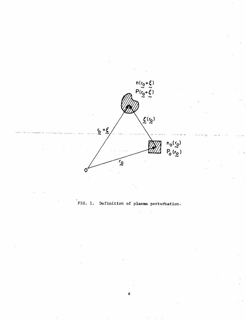
The form of (6) can be understood by reference to Figure 1, and

follows from the fact that when a cell is displaced from r to r +

7

n(ro +)

P(ro+')

O r)no (ro)Po( o

0

FIG. 1. Definition of plasma perturbation.

8

P is defined for the given cell,rather than for the given position, r--0

The adiabatic equation of state must consequently be applied to the same

cell,before and after the displacement. Using the usual definition of

perturbations,

P(r) = P0(r) + P (r) , n(r) = n (r) + n (r) , (7)

and (4), we obtain

P1 = -0P0 v'- I .VP0 (8)

The rf force law in (3) is obtained by comparing the force laws in (1)

and (2) in the same fashion (Newcomb, 1962).

It is now straightforward to use (4), (5), and (8) to rewrite (3)

in terms of only and the rf potential, p1(-l p = E

mnD - (y-l)-P0 g - -

- en0 ( + 'VV 0 - XB) = 0 ,

2

0 v 1 + eV(no) = 0 (9)

Equations in (9) can be Fourier-transformed, normalized, and expressed

in a cylindrical coordinate system, (r,6), for a column of cylindrical

symmetry,

2 Oc+r + A , 2 C r r + 1 er) f'

2r I Yr 1 r5) (@~ +

+ r f rR 1) = O , (10)

1+ A. 2 Yf5( + I _C5 )'C 'r0(0D 2 c r R r R r 1

2 2f 1Pt + e

a A cfr+tD _ r(CO) D +(C Rr R e+ f( + 1 0 , (11)

9

2

(R)'- 1 + (Rf )' f = 0 , (12)1 +R

where the derivative with respect to R is denoted by (') and

0 (O) = o , = r r + (i0O 0

1 (R,O,T) =dQ 1 (R)exp i(QT+ZO) , (13)

with I denoting unit vectors. The normalized quantities are defined as

R= r/a , T= pt , =/ ,

Oc =eBO/nR p , = a ,

2 2 2 2 2 2AD D/a = 0KTe/nO(0)ea , = P 0/n 0(0)ea , (14)

and a static axial magnetic field, BO , has been included.

2.1 Lagrangian Density

The forms of the force law in (3),and the rf pressure in (7) ,

represent the important differences from the paper by Parker, et al. (1964)

in that they make (9),as well as (10)-(12),systems of Euler-Lagrange

equations without having to restrict the values of 7 (Barston, 1965).

In one of the models used by Dorman (1969), an appropriate pressure term

similar to (7) was used without the benefit of the rf force law in (3).

As a result, he was able to establish the variational principle only for

the one-dimensional case.

The Lagrangian corresponding to (10)-(12) can be shown to be the

following, by straightforward application of Hamilton's variational principle,

10

2 2o

11

A f RdR (ICrI2 + II),B =f RdR (CA + CC0f

0f

H -A 2(7T+T') V VS - I+F+F' < 0

0

1

T' fRdR +~ C* + C

0

2 ~Ec + + C-C.3R=1

S ffRdR (Ir2 + 1 Ic91 2

0

11

-f RdR (C + + ,.C F- =J RdR ( t2 - 1R

0 0

R b RC

F/ = f ERdR ( I 2 ~ ~ 2 + Rb RdR ( I 2 11~ 2)0 R bR

b R (15)

where c.c. denotes complex conjugate. Equation (15) is appropriate

to the configuration shown in Figure 2 of a concentric metal cylinder

surrounding a glass tube, of relative permittivity E , that containsg

the plasma column. In the expressions for T and T' , the boundary

terms are included to modify the natural boundary conditions on C

and ( (see for example, Courant and Hilbert, 1953) that would other-

with be unphysical. In the expressions for H and S , C0 (r) and VO

are defined as

¢ 0 (r) = - 0(r)/V 0 , V0 =- (a)

Substitution of the exact solutions of (10)-(12) would make 2(,)

zero. We see from (15) that, for negligible Oc ' D , and VO , the

resonance frequencies are determined essentially by the values of I, F,

and F' . Since V0 is approximately proportional to AD (Self, 1963;

Parker, 1963), the effect of higher electron temperature is to raise each

resonance frequency. When nc 0 , the roots of £ 2(O,t) = 0 are

B,2 =cB/2A [(QcB/2A)2 - H/A]1/ 2 (16)

Since Q and- O are indistinguishable in experimental observations, we

see that all the resonance frequencies are predicted by (16) to split

in two,in agreement with the theoretical results of Barston (1965), and

Vandenplas and Messiaen (1965). For sufficiently small Oc , when thec

values of B and A are not greatly affected by the presence of an

axial static magnetic field, the amount of the split, B/AI , will

be proportional to Oc. This is in agreement with the observed splitting

character of the main dipole resonance frequencies (Crawford, Kino, and

Cannara, 1963; Messiaen and Vandenplas, 1962). Furthermore, since

A z IBI, where the equal sign applies when C C e , this split is predicted

to be always less than or equal toc

12

FIG. 2. Plasma column geometry.

13

2.2 Rayleigh-Ritz Procedure and Coordinate Functions

For a single linear Euler-Lagrangian equation, the Rayleigh-Ritz

procedure is efficient in obtaining an approximate solution,by use of a

weighted summation of a set of judiciously chosen coordinate functions.

These coordinate functions must be linearly independent and complete,

and satisfy the boundary conditions specified by the problem. The

weighting coefficients that appear in the approximated Lagrangian are

varied independently. This results in a system of algebraic equations

that take the place of the original equation. Theoretically, better

approximations can be obtained by using more coordinate functions. When

eigenvalues are involved, the approximate eigenvalues always converge to

the exact values from above (see for example, Mikhlin, 1964).

Much less attention has been given to the analogous problem for a

system of linear Euler-Lagrangian equations, e.g. (10)-(12), though the

theoretical extension of the variational method to a system of second order

elliptic equations has been mentioned by Mikhlin (1965): the way to set

up the corresponding coordinate functions is similar to that for the single

equation case, i.e. the coefficients of each dependent variable are varied

independently.

For our problem, in which (10)- (12) are not in elliptic form, the

coordinate functions and the coefficients must be more restricted. In the

Appendix to the paper it is shown that acceptable estimates of resonance

frequencies and eigenfunctions can be obtained for our problem provided

that the coordinate functions chosen for each dependent variable are

related by (10)-(12).

By expanding Cr C , and l in power series of R, and substituting

in (10)-(12), we see that for small R , C = C r R - 1 , and Wl = R.

14

Thus, for . 1 , the solutions are well behaved at R = 0 . If we

also choose even functions for f(R) and o(R) , then Cr and C. are

even in R , and 1 is odd in R , when ( is odd, and vice versa.

Since there are no other singularities in (10)-(12), polynomials in R

constitute appropriate coordinate functions for our problem. For convenience,

the coordinate functions chosen for Cr will be

r = R - R+2j-1 (j = 1,2,...) , (17)

which conform to the usual assumption of zero normal rf current, since

Crj(1) = 0

Rather than choosing C j and lj independently, we must determine

them via the original differential equations and (17). After eliminating

(1 in (10) and (11), it follows by using the second equation of (4) that

R2 (RC + C - r ) = [R Ocn + ((-1) 0 ](Rr + ~-i) . (18)

With a given expression for 0(r) , and an assigned value of 2 , e.g.

= 1 , j can then be easily determined for any given rrj

An immediate question arises concerning the dependence of the resulting

variational estimate of resonance frequencies on the size of n chosen

arbitrarily here. We have found that the first few resonance frequencies

-4do not change by more than 10 w when 0 in (18) changes from 0.4 to 1

p2

for all the values of 1/AD used in this paper. If this were not the

case, an iterative procedure would have to be used, i.e. the resulting

variational estimate of Q would have to be used in (18) to obtain a

new set of ,j . These would be used in turn to obtain improved frequency

estimates, and so on.

The corresponding coordinate function, lj , is obtained by solving

(12) (Barston, 1965),with conditions of continuity of potential and normal

displacement across the boundaries defined in Figure 2. According to the

15

discussion given in the Appendix, identical coefficients are assigned to

each set of coordinate functions,

N N N

r = aj Crj C0 = ajj , D1= aj,j , (19)

j=1 j=1 j=1

before substitution in the Lagrangian, 2(M,tf), of (15). The resulting

Lagrangian then gives the algebraic Euler-Lagrange equation below,

NS(02A.. -'QQ B + H )a. = 0 (i = 1,2,... , N)c Ji ji I

1

A ij fRdR(Cri rj + 'oiej) , (20)

where Aij , Bij , and Hij are the matrix elements of the integrals, A,

B, and H, given in (15), respectively, and are obtained by substituting

the coordinate functions in a fashion given by the above A.. expression.1j

Equation (20) can be transformed into a generalized eigenvalue problem

(Dorman, 1969)

2N

(QA. - B.j)b = 0 (i = 1,2,... , 2N)

j=1

b. = (a ,ai) (j = 1,2,..., 2N, i 1,2, .. N)

A-HS= B -H (21)

with superscript + signifying the transposition of a matrix. Equation (21)

is now solvable by standard computer codes.

16

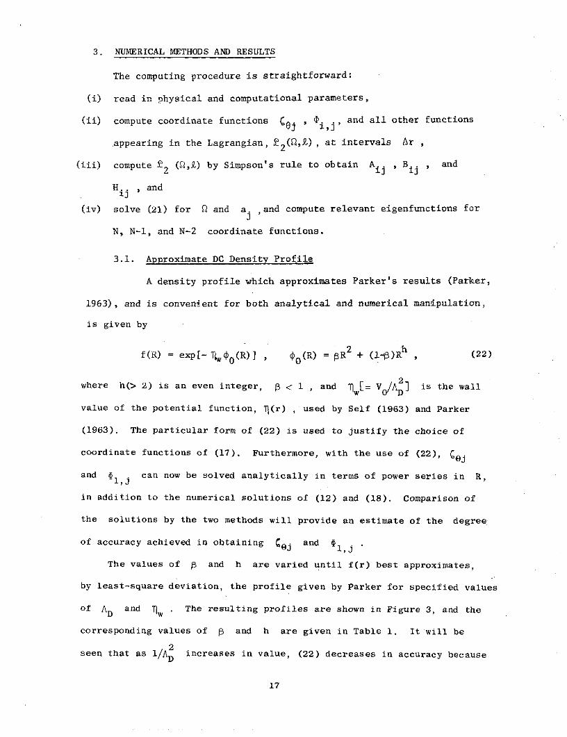
3. NUMERICAL METHODS AND RESULTS

The computing procedure is straightforward:

(i) read in physical and computational parameters,

(ii) compute coordinate functions Cj ', i,j' and all other functions

appearing in the Lagrangian, £22 (Q,) , at intervals Ar ,

(iii) compute 22 (,Z) by Simpson's rule to obtain Aij , Bij , and

H.. , and

(iv) solve (21) for 0 and a. and compute relevant eigenfunctions for

N, N-I, and N-2 coordinate functions.

3.1. Approximate DC Density Profile

A density profile which approximates Parker's results (Parker,

1963), and is convenient for both analytical and numerical manipulation,

is given by

f(R) = exp[- w 0 (R)] , g0 (R) = R 2 + (13)Rh , (22)

where h(> 2) is an even integer, p < 1 , and Tw[= Vo/AI ] is the wall

value of the potential function, q(r) , used by Self (1963) and Parker

(1963). The particular form of (22) is used to justify the choice of

coordinate functions of (17). Furthermore, with the use of (22), (j

and l,j can now be solved analytically in terms of power series in R,

in addition to the numerical solutions of (12) and (18). Comparison of

the solutions by the two methods will provide an estimate of the degree

of accuracy achieved in obtaining Cej and §l,j

The values of 1 and h are varied until f(r) best approximates,

by least-square deviation, the profile given by Parker for specified values

of AD and w . The resulting profiles are shown in Figure 3, and the

corresponding values of p and h are given in Table 1. It will be

seen that as l/AD increases in value, (22) decreases in accuracy because

17

f(R) f (R)

(a) (d)

(b) (e)

SI 0 I

FIG. 3. Comparison between (22) (indicated by dots), and Parker's

density profile, for the parameters given in Table 1.

Table 1

Parameters used in (22), and Figure 3, for a mercury-vapor

positive column. The conversion between 1/A 2 and 1A2

is obtained by the calculations of Parker (1963).

2 2* 2 21/A D/A, B h 2, tER

2 1 * -4a 3.4 X 102 7.2 X 101 6.72 0.447 4 6.2 X 10

3 2 -4b 1.3 X 10 5.1 X 10 6.60 0.221 8 1.3 X 10

c 8.2 X 103 4.5 X 103 6.52 0.159 20 t6.2 X 10-4

d 6.7 x 104 4.3 X 104 6.44 0.142 54 t2.9 X 10- 3

5 5 -3e 6.2 x 10 4.2 X 105 6.40 0.141 156 t7.5 X 10

f O 1.08 0.644 12 tl.3 X 10-4

19

of the increasing degree of steepness displayed by the density profile

in the sheath region. At zero temperature, the sheath is omitted and

an accurate approximation can again be obtained. The approximation of

(22), however, was found to be sufficient to give accurate frequency

and eigenfunction estimates for all of the values of 1/AD listed in

Table 1.

20

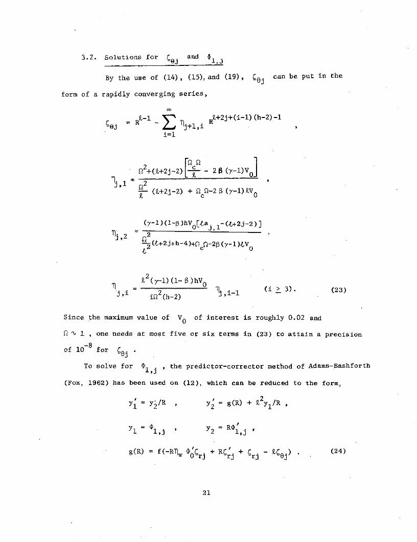
3.2. Solutions for COj and lj

By the use of (14), (15), and (19), 5Cj can be put in the

form of a rapidly converging series,

00

--1 Ij+1,i R +2j+(i-1) (h-2)-1

i=l

2+(t+2j-2) - 28 ( 7 -1)V0J

j,1 2

-- (a+2j-2) + 0 c-2 (7-1)£V0

(7-1) (1-p)hVOaj, 1 -(,Q+2j-2) ]

1,2 22 (t+2j+h-4)+pc -2p (7-1)lV0

£2( 7-1)(1- B)hV0

ji 2(h2) ,i- (i 3) (23)

Since the maximum value of V0 of interest is roughly 0.02 and

Q '% 1 , one needs at most five or six terms in (23) to attain a precision

-8of 10 for C j .

To solve for ,j , the predictor-corrector method of Adams-Bashforth

(Fox, 1962) has been used on (12), which can be reduced to the form,

YI = y /R , 2 = g(R) + 2 yl/R

y = , y=R1 l,j ' Y 2 ,j

g(R) = f(-R 0j + RCj + rj - £ j) (24)rj r21 rj j

21

N N RSince the complementary solution of (24) is 1lj = Y = , and its

P R +2jparticular solution, yl is proportional to R near r = 0 ,

yl (0) and y2 (0) are both equal to zero. So the starting values of

P PYl and Y2 are well-behaved, and easily obtained by Taylor

series

expansion near R = 0 . The total solution of l,j can then be written

as

,j = c.R + , (25)1, J 1,j

where c is determined by imposing the boundary conditions of m1

By making the interval Ar = 0.01, and using double precision, ij

can be calculated to within 10 - 8 . This is arrived at, first, by com-

paring results that use different values of Ar , and secondly, checking

against solutions of (12) obtained by power-series expansions in R

3.3 Numerical Instability

In the process of solving the algebraic equation,(21), the size

of N is limited by the inaccuracy involved in obtaining Aij , etc.

This inaccuracy introduces a numerical instability whenever the coordinate

functions are not orthogonal functions with respect to the differential

operators of (10)-(12) (Mikhlin, 1971, Chap. 2). The situation is best

illustrated by an example in which the dipole resonance frequencies

corresponding to Figure 3(b) are calculated for different values of N

while holding the size of Ar constant at 0.05.

As shown in Table 2, as N is increased from 2 , the first few

resonance frequencies are approached from above with rapidly stabilized

estimates. When N is increased beyond 8, undesirable fluctuations

-4larger than 10- 4 , and clearly erratic changes in the values of Q , start

to appear. In the case N = 9, for example, one would obtain an erroneous

22

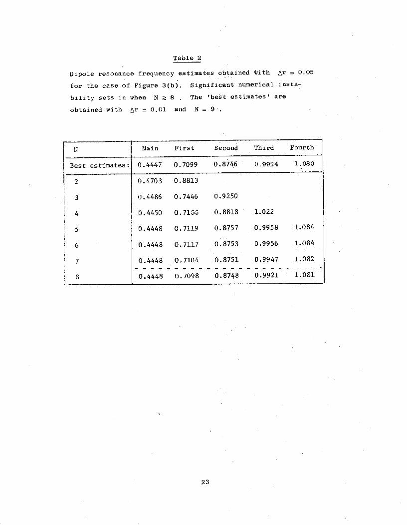
Table 2

Dipole resonance frequency estimates obtained With Ar = 0.05

for the case of Figure 3(b). Significant numerical insta-

bility sets in when N 2 8 . The 'best estimates' are

obtained with Ar = 0.01 and N = 9-.

N Main First Second Third Fourth

Best estimates: 0.4447 0.7099 0.8746 0.9924 1.080

2 0.4703 0.8813

3 0.4486 0.7446 0.9250

4 0.4450 0.7155 0.8818 1.022

5 0.4448 0.7119 0.8757 0.9958 1.084

6 0.4448 0.7117 0.8753 0.9956 1.084

7 0.4448 0.7104 0.8751 0.9947 1.082

8 0.4448 0.7098 0.8748 0.9921 1.081

23

fundamental resonance frequency. Characteristic of the variational

nature of the Lagrangian, £2(Q,t), more serious errors are found in

the approximate eigenfunctions, than in the resonance frequencies. The

optimal combination of N and Ar , that produces acceptable results

in the shortest computation time, can be obtained by trial and error.

Repeated solution of (21) for a few adjacent values of N thus becomes

an economical technique: this requires computation of the matrices A. ,

etc. only once, and offers safeguards against obtaining erroneous results

due to numerical instabilities.

3.4 Computer Results

As a practical example, the approximate density profiles given

in Table 1 have been used to predict dipole resonances for Tube No. 1

used by Parker, et al. (1964) ( = 1; a = 0.5 cm; effective relative

permittivity at the surface of the column Keff i/ 1 = 2.1). The

computation time varies roughly as N2 . With N = 10, a typical calcu-

lation takes about 40 seconds, and requires a core space of less than

100K 'bytes in an IBM 370/67 machine.

The resulting approximate solutions for gri 6, l' p1 , and

are plotted in Figures 4-6. The density and the radial electric field

solutions, n (R) and p' resemble very closely those given by Parker, et al.

(1964), and Parbhakar and Gregory (1971), respectively. The relative

amplitudes of r and .e shown in these figures are retained, revealing

that as l/AD increases, r progressively dominates over O. For

1/AD > 4500 , it will be seen that the perturbations should be progressively

compressed toward the sheath region as l/AD increases in value. These

24

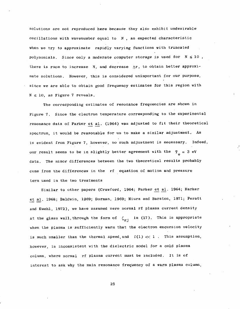
solutions are not reproduced here because they also exhibit undesirable

oscillations with wavenumber equal to N , an expected characteristic

when we try to approximate rapidly varying functions with truncated

polynomials. Since only a moderate computer storage is used for N 10 ,

there is room to increase N, and decrease /r, to obtain better approxi-

mate solutions. However, this is considered unimportant for our purpose,

since we are able to obtain good frequency estimates for this region with

N : 10, as Figure 7 reveals.

The corresponding estimates of resonance frequencies are shown in

Figure 7. Since the electron temperature corresponding to the experimental

resonance data of Parker et al. (1964) was adjusted to fit their theoretical

spectrum, it would be reasonable for us to make a similar adjustment. As

is evident from Figure 7, however, no such adjustment is necessary. Indeed,

our result seems to be in slightly better agreement with the Te = 3 eV

data. The minor differences between the two theoretical results probably

come from the differences in the rf equation of motion and pressure

term used in the two treatments

Similar to other papers (Crawford, 1964; Parker et al. 1964; Harker

et al. 1968; Baldwin, 1969; Dorman, 1969; Miura and Barston, 1971; Peratt

and Kuehl, 1972), we have assumed zero normal rf plasma current density

at the glass wall,through the form of Crj in (17). This is appropriate

when the plasma is sufficiently warm that the electron excursion velocity

is much smaller than the thermal speed,and f(l) << 1 . This assumption,

however, is inconsistent with the dielectric model for a cold plasma

column, where normal rf plasma current must be included. It is of

interest to ask why the main resonance frequency of a warm plasma column,

25

RESONANCES

MAIN I st

FIG. 4. Approximate solutions for 1/) = 72, R = 1

26

RESONANCESMAIN I st 2nd

4-

SI II

FIG. 5. Approximate solutions for 1/ = 510, =

27

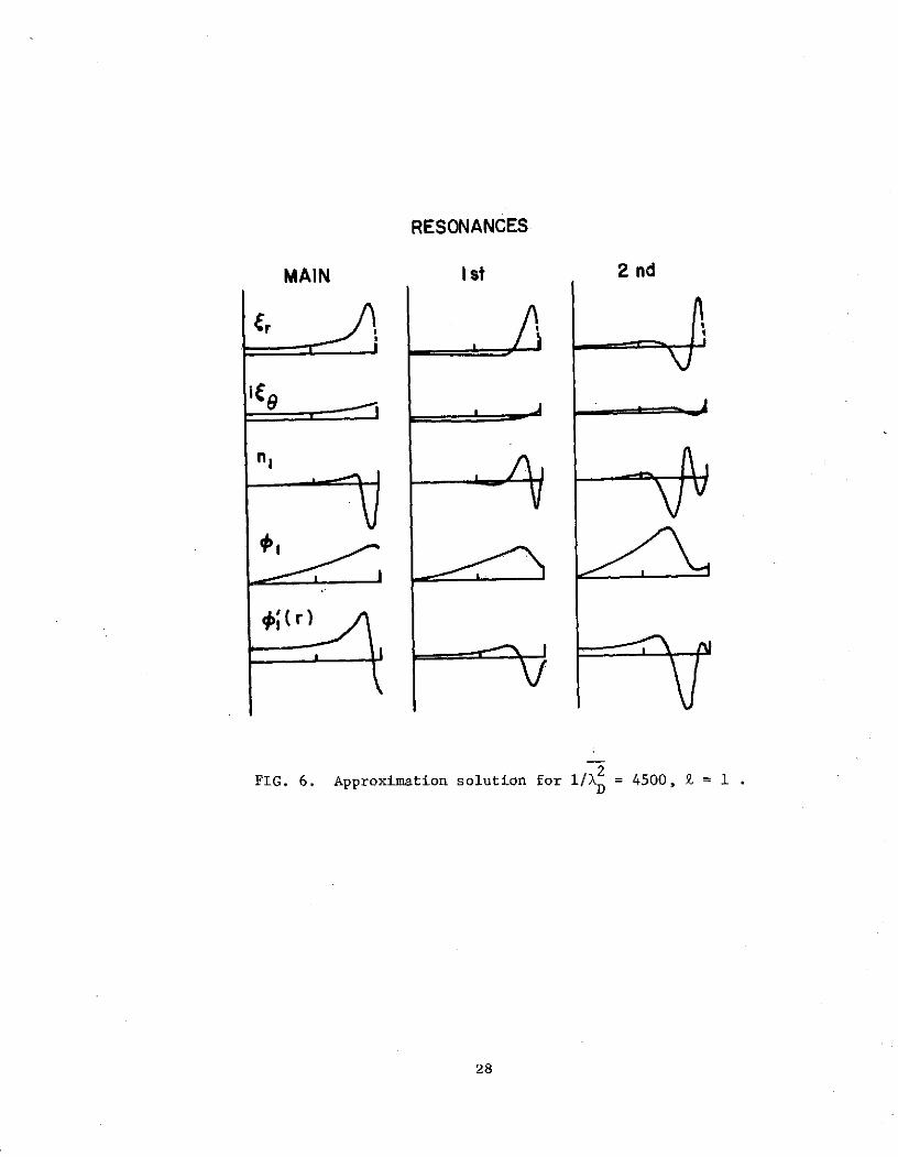
RESONANCES

MAIN Ist 2 nd

Cr

FIG. 6. Approximation solution for 1A/X = 4500, £

28

3.0TUBE NO. I-DIPOLE

\ a = 0.5 cm

\ K ff= 2 .I

2.0- o+ Te 3eV

0 2ndW30

N-o

1.0 %+

o -MAIN

1 /A

FIG. 7. Dipole resonance spectrum of Tube No. 1 (Parker et al.), compared with

estimates by the variational method (indicated by crosses).

in the limit of low temperature, approaches the principal resonance of

a cold plasma column. To answer this question, we need only change (17)

to

R-1i RC+2j-1(rj = R +2j- (j = 1,2,...) , (26)

and impose the requirement of continuity of normal displacement in the

form

1(1 ) + f(1)Cr(1) = E W(1 ) (27)

The resulting solutions of Cr are found to be only slightly different

from the previous case near R = 1 [Figures 4-6, where the dashed lines

correspond to the use of (17)]. Furthermore, the main resonance is

lowered by less than 1 per cent for all of the values of I/AD used

here, including the case l/AD - a . This is well within the experi-

mental errors.

30

4. DISCUSSION

In this paper, we have applied the Rayleigh-Ritz procedure to a system

of three Euler-Lagrangian equations that describe the electron resonances

of a nonuniform warm plasma column. It is shown that accurate frequencies

for the first few resonances can be obtained for the entire range of

l/A >> 1 . Results which agree closely with those of Parker, et al.

(1964) have been obtained

Contrary to the case of a system of elliptic equations, where the

coefficients are assigned independently to each dependent variable

(Mikhlin, 1971), we have found that for (10)-(12), the same coefficient

must be assigned to each set of coordinate functions, e.g. (19). In

addition to the usual requirements,that the coordinate functions must be

linearly independent and complete, we have chosen that they be set up in

accordance with (10)-(12).

The present method can be easily modified to include the effects

of electron dc drift, dc magnetic field, and ion motion. With the axial

dimensions and rf magnetic field included, this procedure would be efficient

in solving travelling wave problems in a nonuniform plasma waveguide.

31

ACKNOWLEDGMENTS

The authors are indebted to Drs. K. J. Harker and H. Kim for many

useful discussions. The work was supported by the National Aeronautics

and Space Administration.

32

REFERENCES

Baldwin, D. E. 1969, Phys. Fluids, 12, 279.

Barston, E. M. 1963, Phys. Fluids, 6, 828.

Barston, E. M. 1965, Phys. Rev., 139, A394.

Briggs, R. J. and Paik, S. F. 1968, Int. J. Electron., 23, 163.

Courant, R. and Hilbert, D. 1953, Methods of Mathematical Physics, Vol. 1,

Interscience, p. 208.

Crawford, F. W., Kino, G. S. 1963, C. R. Hebd. Seanc. Acad. Sci.,

Paris, 256, 1939 and 2798.

Crawford, F. W., Kino, G. S. and Cannara, A. B. 1963, J. Appl. Phys.,34,

3168.

Crawford, F. W. 1964, J. Appl. Phys., 35, 1365.

Crawford, F. W. 1965, Int. J. Electron., 19, 217.

Dorman, G. 1969, J. Plasma Phys., 3, 387.

Fox, L. 1962, Numerical Solution of Ordinary and Partial Differential

Equations, Addison-Wesley, p. 29.

Harker, K. J., Kino, G. S., and Eitelbach, D. L. 1968, Phys. Fluids, 11,

425.

Messiaen, A. M. and Vandenplas, P. E. 1962, Physica, 28, 537.

Mikhlin, S. G. 1964, Variational Methods in Mathematical Physics, Pergamon.

Mikhlin, S. G. 1965, The Problem of the Minimum of a Quadratic Functional,

Holden-Day, p. 148.

Mikhlin, S. G. 1971, The Numerical Performance of the Variational Method,

Wolters-Noordhoff.

Miura, R. M. and Barston, E. M. 1971, J. Plasma Phys., 6, 271.

Newcomb, W. A. 1962, Nucl. Fusion, Supplement, Part 2, 451.

Parbhakar, K. J. and Gregory, B. C. 1971, Can. J. Phys., 49, 2578.

33

Parker, J. V. 1963, Phys. Fluids, 6, 1657.

Peratt, A. L., Kuehl, H. H. 1972, Phys. Fluids,15, 1117.

Parker, J. V., Nickel, J. C., and Gould, R. W. 1964, Phys. Fluids, 7,

1489.

Self, S. A. 1963, Phys. Fluids, 6, 1762.

Sturrock, P. A. 1958, Ann. Phys., 4, 306.

Vandenplas, P. E. and Messiaen, A. M. 1965, Nucl. Fusion, 5, 47.

34

APPENDIX

Here we shall show that the coordinate functions, C rj 0j , and

lJj ' must be assigned the same coefficients, aj , for the Rayleigh-

Ritz procedure applied to £2 ('t) of (15) to be successful: it will

be shown that, by restricting these coordinate functions according to

(10)-(12), the appropriate Rayleigh-Ritz procedure can be established.

A system of second order elliptic equations can be written as

(DjkU)' + XE U = 0 , Djk = Dkj Ejk = Ekj , (A.1)jk k jk jk kj jk kj

where U k is the k th dependent variable, the matrices Djk and Ejk

are functions of the independent variable x , the eigenvalue is X( 0),

and the summation convention has been used. Ellipticity demands that

Djkaja k 0 , Ejk ja k O0 , (A.2)

for any real non-zero vector c. . The solutions of (A.1) then admit

of variational estimates, as outlined by Mikhlin (1965).

When we apply the Rayleigh-Ritz procedure to the Lagrangian for (A.1),

1

L= fdx (DjkUU - X EjkUjU k) , (A.3)

0

the coefficients preceding the coordinate function for each U k can be

varied independently. Suppose a set of legitimate trial functions,

Uk = CkVk (summation convention not used here) with coefficient Ck , are

used in (A.3). Because of (A.2),we can obtain crude estimates of X

larger than the lowest eigenvalue,even if only one of the C k is non-zero.

If the same procedure is applied to the Lagrangian in (15), we will

obtain erroneous estimates of 0 . Consider the case of a cold, uniform

plasma column with BO = O , so that H = -I + F + F' Suppose Cr '

35

C ,and C are the coefficients for the coordinate functions rj ,

r , and , respectively. Then if C = 0 , the value of the

estimate will be zero, and fail the requirement of the Rayleigh-Ritz

sequence.

Consequently, to make (-H/A) 1/2 from (15) at least non-zero, we

must use a single coefficient for each set of the coordinate functions

rj and . Merely making C = C = C = a. is insuffi-rjMerely making Cr

cient to produce a legitimate Rayleigh-Ritz sequence, because the value

of lj , for example, can be arbitrarily small in comparison with

Crj and C6j , making the Q estimates also arbitrarily small. We

see that restricting these coordinate functions according to (10)-(12),

is sufficient to reduce the resulting approximated Lagrangian to a single

Euler-Lagrange equation. The appropriateness of the resulting Rayleigh-

Ritz procedure can then be guaranteed. It is conceivable, of course,

that there may be less restrictive choices of appropriate coordinate

functions corresponding to the Lagrangian in (15), but we have not chosen

to pursue this point.

36