variable selection in multiple linear regression: the
TRANSCRIPT

Volume 23 (2), pp. 123–136
http://www.orssa.org.za
ORiONISSN 0529-191-X
c©2007
Variable selection in multiple linear regression: Theinfluence of individual cases
SJ Steel∗ DW Uys†
Received: 31 May 2006; Revised: 23 April 2007; Accepted: 25 April 2007
Abstract
The influence of individual cases in a data set is studied when variable selection is applied inmultiple linear regression. Two different influence measures, based on the Cp criterion andAkaike’s information criterion, are introduced. The relative change in the selection criterionwhen an individual case is omitted is proposed as the selection influence of the specific omittedcase. Four standard examples from the literature are considered and the selection influence ofthe cases is calculated. It is argued that the selection procedure may be improved by takingthe selection influence of individual data cases into account.
Key words: Akaike’s information criterion, influential data cases, Mallows’ Cp criterion, multiple
linear regression, variable selection.
1 Introduction
The literature on statistical variable selection, frequently one of the first steps in a multi-ple linear regression analysis, is considerable. Recent references are Burnham & Anderson(2002) and Murtaugh (1998). The purpose of regression variable selection is to reduce thepredictors to some “optimal” subset of the available regressors. This may be importantbecause (i) a smaller set of predictors may provide more accurate predictions of futurecases, or, (ii) it may be important to identify those predictor variables significantly influ-encing the response (for example, in a clinical trial). There are many techniques whichare routinely used for variable selection in multiple linear regression: stepwise routinessuch as forward selection (Miller, 2002), Bayesian techniques (an extensive list of refer-ences is given in Burnham & Anderson, 1998, p.127), cross-validation selection techniques(Liu et al., 1999), or an all possible subsets approach based, for example, on Mallows’ Cp
criterion (Mallows, 1973, 1995), or Breiman’s little bootstrap (Breiman, 1992; Venter &
∗Department of Statistics and Actuarial Science, University of Stellenbosch, Private Bag X1, Matieland,7602, South Africa.
†Corresponding author: Department of Statistics and Actuarial Science, University of Stellenbosch,Private Bag X1, Matieland, 7602, South Africa, email: [email protected].
123

124 SJ Steel & DW Uys
Snyman, 1997). In this paper attention is restricted to selection using an all possible sub-sets approach based on either the Cp criterion or Akaike’s information criterion (Akaike,1973).
The literature on measures of the influence of individual cases in a data set on a multiplelinear regression fit is equally impressive. Some contributions include Cook (1977, 1986),and Belsley et al. (1980). These and other contributions on influence measures assumethat the predictor variables are identified beforehand. If an initial selection step takesplace, the influence measures are therefore conditional, i.e. the specific predictors in themodel are given.
Only a few papers dealing with the influence of individual data cases in regression explic-itly take an initial variable selection step into account. In this context, Leger & Altman(1993) distinguish between conditional and unconditional selection versions of Cook’s dis-tance. To explain the difference between the two versions, let V be the set of indicescorresponding to the predictor variables selected from the full data set, and let _
y (V ) bethe prediction vector based on the selected variables and calculated from the full data set.Also, let _
y (−i) (V ) be the prediction vector based on the variables corresponding to V , butcalculated from the full data set without case i. Note that _
y (−i) (V ) contains a predictionfor case i, although this case is not used in calculating _
y (−i) (V ). The conditional Cook’sdistance for the i-th case is ∥∥∥_
y(V )− _y (−i) (V )
∥∥∥2,
appropriately scaled. Here, ‖•‖ denotes the Euclidean norm. To obtain the unconditionalCook’s distance, Leger & Altman (1993) argue that it is necessary to repeat the variableselection using the data without case i. This selection yields a subset V(−i) of indices, withV(−i) possibly different from V . The unconditional distance is
∥∥∥_y(V )− _
y (−i)
(V(−i)
)∥∥∥2,
appropriately scaled. Leger & Altman (1993) discuss the differences between these twoselection versions of Cook’s distance and argue that the unconditional version is preferable,since it explicitly takes the selection effect into account.
In this paper we introduce two new measures of the selection influence of an individual datacase in multiple linear regression analysis. Our point of view is that such a measure shouldprovide an indication of whether the fit of the selected model improves or deterioratesowing to the presence of the case. This is the main contribution of the paper. Section 2is devoted to a brief exposition of Mallows’ Cp statistic and Akaike’s information criterion(AIC ). The new measures of selection influence, based on Cp and AIC respectively, areintroduced in Section 3. It is indicated how variable selection based on Cp or on AICmay be modified, and hopefully improved, by making use of the influence measures. Fourpractical examples are discussed in Section 4. We close with some recommendations inSection 5.

Variable selection in multiple linear regression: The influence of individual cases 125
2 Variable selection using Cp or AIC
Let y1, . . . yn be observations of the response in a multiple linear regression, with corre-sponding observations xij , i = 1, . . . , n; j = 1, . . . , p of p explanatory variables. We makethe customary assumption that
yi = β0 +p∑
j=1
βjxij + εi, (1)
for i = 1, . . . , n. In (1), ε1, . . . , εn are independent normal(0;σ2
)random variables, and
β0, . . . , βn and σ2 are unknown parameters. We assume that {xi1, . . . , xip} may containredundant variables, so that it is advisable to perform variable selection as a first step inthe analysis. Let RSS be the residual sum of squares from the least squares fit of (1).Then σ2 = RSS/(n − p − 1) is the commonly used unbiased estimator of σ2. Considera subset V of {1, . . . , p}, and let RSS(V ) be the residual sum of squares from the leastsquares fit using only the regressors corresponding to the indices in V , together with anintercept. The Cp statistic for the corresponding model is
Cp (V ) =RSS(V )
σ2+ 2(v + 1) − n, (2)
where v is the number of indices in V . Variable selection based on (2) entails calculatingCp (V ) for each subset of {1, . . . , p}, and selecting the variables corresponding to V , thesubset minimizing (2). This approach is based on the fact that for a given V , σ2Cp (V ) isan estimate of the expected squared error if a (multiple) linear regression function basedon the variables corresponding to V is used to predict Y ∗, a new (future) observation ofthe response random vector, Y . Therefore, choosing V to minimize (2) is equivalent toselecting the variables which minimize the estimated expected prediction error.
The AIC is based on the maximized log-likelihood function of the model under consid-eration. Given independent normal errors, and ignoring constant terms, the maximizedlog-likelihood for the model corresponding to a subset V is given by −n log [RSS(V )/n] /2.This is a non-decreasing function of the number of selected regressors. Akaike (1973) there-fore included a penalty term, viz. v + 2, which equals the number of parameters whichhave to be estimated. Multiplying the resulting expression by −2 yields
AIC(V ) = n log(
RSS(V )n
)+ 2(v + 2). (3)
For an up-to-date discussion and further motivation of (3), see Burnham and Anderson(2002). It is known that AIC(V ) does not perform well when the number of parameters tobe estimated is large compared to the sample size (typically cases where 40 (v + 2) > n).In such cases a modified version of (3) should be used, viz.
AIC(V ) = n log(
RSS(V )n
)+
2n (v + 2)n − v − 3
. (4)
Variable selection based on (3) or (4) entails calculating the criterion for each subset Vof {1, . . . , p}, and selecting the variables corresponding to the minimizing subset. This isequivalent to selecting the variables which maximize a penalized version of the maximumlog-likelihood.

126 SJ Steel & DW Uys
3 New measures of selection influence
It is standard statistical practice in multiple linear regression to study the influence of asingle data case in an analysis as follows: analyse the complete data set and calculate a(summary) measure, say M ; repeat the analysis after omitting the case under considerationand calculate M(−i); quantify the influence of case i in terms of a function, f(•), of M andM(−i). An example is provided by Cook’s statistic, where M is the vector of predictionsof the response, and f(x) = ‖x‖2 /RSS.
The measures of selection influence which we propose are also based on a leave-one-outstrategy. The following questions need to be resolved: (i) What is meant by an analysisof the complete or reduced data set? (ii) What measure M should be used? (iii) Howshould we define f(•)? Regarding the first question, in a variable selection context ananalysis of a data set entails applying a given variable selection technique, and fitting themodel corresponding to V to the data. Consequently, if we wish to study the influenceof a single data case in such an analysis, it is necessary to apply the selection techniqueunder consideration to the full data set and again to the reduced data set. This is in linewith the unconditional approach recommended by Leger and Altman (1993). Turning tothe second question, different choices of M can be made, depending on the aspect of thefitted model which is of interest. In variable selection the number of selected variablesand the lack of fit of the corresponding model are typically of interest. These quantitiesare combined in selection criteria such as Cp and the AIC. It therefore seems reasonableto take M equal to the criterion employed in the selection method. This implies thatf(•) has to be based on the difference in the value of the selection criterion before andafter omitting case i. This difference, M − M(−i), may then be divided by M in order tocalculate the relative change in the selection criterion. The proposed selection influencemeasure for the i-th case is therefore given by
f(M,M(−i)
)=
M −M(−i)
M, (5)
where M denotes the selection criterion under consideration. Note that (5) may be calcu-lated for all selection criteria where the particular criterion is a combination of some sortof goodness-of-fit measure and a penalty function (such a penalty function usually includesthe number of predictors of the particular selected model as one of its components, seeKundu and Murali (1996)).
The proposed influence measure for the i-th case when the Cp criterion is used becomes
f(Cp (V ) , Cp
(V(−i)
)) =
Cp (V )− Cp
(V(−i)
)Cp (V )
, (6)
where Cp
(V(−i)
)is calculated as in (2), but with the i-th case omitted. Note that in
calculating Cp
(V(−i)
)the estimator for the error variance is obtained from the full data
set. The use of this error variance estimator is supported by considerations given by Legerand Altman (1993) for using σ2 in the denominator of the unconditional Cook’s distance.The proposed influence measure based on the Cp criterion in (6) is large if the relativedifference between Cp (V ) and Cp
(V(−i)
)is large. If this is true for an omitted data
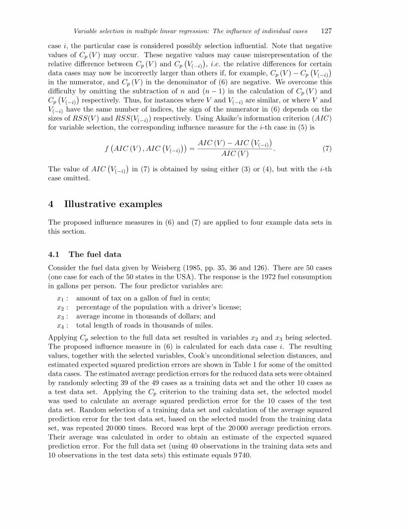
Variable selection in multiple linear regression: The influence of individual cases 127
case i, the particular case is considered possibly selection influential. Note that negativevalues of Cp (V ) may occur. These negative values may cause misrepresentation of therelative difference between Cp (V ) and Cp
(V(−i)
), i.e. the relative differences for certain
data cases may now be incorrectly larger than others if, for example, Cp (V ) − Cp
(V(−i)
)in the numerator, and Cp (V ) in the denominator of (6) are negative. We overcome thisdifficulty by omitting the subtraction of n and (n − 1) in the calculation of Cp (V ) andCp
(V(−i)
)respectively. Thus, for instances where V and V(−i) are similar, or where V and
V(−i) have the same number of indices, the sign of the numerator in (6) depends on thesizes of RSS(V ) and RSS(V(−i)) respectively. Using Akaike’s information criterion (AIC )for variable selection, the corresponding influence measure for the i-th case in (5) is
f(AIC (V ) , AIC
(V(−i)
))=
AIC (V )−AIC(V(−i)
)AIC (V )
. (7)
The value of AIC(V(−i)
)in (7) is obtained by using either (3) or (4), but with the i-th
case omitted.
4 Illustrative examples
The proposed influence measures in (6) and (7) are applied to four example data sets inthis section.
4.1 The fuel data
Consider the fuel data given by Weisberg (1985, pp. 35, 36 and 126). There are 50 cases(one case for each of the 50 states in the USA). The response is the 1972 fuel consumptionin gallons per person. The four predictor variables are:
x1 : amount of tax on a gallon of fuel in cents;x2 : percentage of the population with a driver’s license;x3 : average income in thousands of dollars; andx4 : total length of roads in thousands of miles.
Applying Cp selection to the full data set resulted in variables x2 and x3 being selected.The proposed influence measure in (6) is calculated for each data case i. The resultingvalues, together with the selected variables, Cook’s unconditional selection distances, andestimated expected squared prediction errors are shown in Table 1 for some of the omitteddata cases. The estimated average prediction errors for the reduced data sets were obtainedby randomly selecting 39 of the 49 cases as a training data set and the other 10 cases asa test data set. Applying the Cp criterion to the training data set, the selected modelwas used to calculate an average squared prediction error for the 10 cases of the testdata set. Random selection of a training data set and calculation of the average squaredprediction error for the test data set, based on the selected model from the training dataset, was repeated 20 000 times. Record was kept of the 20 000 average prediction errors.Their average was calculated in order to obtain an estimate of the expected squaredprediction error. For the full data set (using 40 observations in the training data sets and10 observations in the test data sets) this estimate equals 9 740.

128 SJ Steel & DW Uys
Case Variables Influence Unconditional Averageomitted selected measure Cook’s distance prediction error
1 2,3 0.0016 0.0017 9 90912 2,3 0.0004 0.0007 10 06113 2,3 0.0006 0.0004 10 10019 2,3 0.0557 0.1986 9 51328 2,3 0.0009 0.0005 9 97232 2,3 0.0005 0.0008 9 92433 2,3 0.0224 0.0486 9 81139 2,3 0.0192 0.0402 9 75640 2,3,4 0.2038 0.8756 8 01345 2,3 0.0652 0.1627 9 32949 2,3,4 0.1024 1.0664 8 68850 1,2,3 0.2658 2.4029 6 057
Table 1: Fuel data: Variable selection with Mallows’ Cp criterion.
It is clear from Table 1 that the proposed influence measure and Cook’s unconditionaldistance are relatively large when case 40, 49 or 50 is omitted. Both reach a maximumwhen data case 50 is omitted. We observe a sharp reduction in the estimated averageprediction error (from 9 740 to 6 053) for the reduced data set where case 50 is omitted.The estimated average prediction errors for the reduced data sets without case 40 or 49are also considerably smaller than that of the full data set, but not as low as that of thereduced data set with case 50 omitted. It would therefore seem to be advisable to omitdata case 50 before performing variable selection and model fitting on the fuel data. Notethat variables x1, x2 and x3 are selected if case 50 is omitted.
There is a strong correspondence between the values of the proposed influence measure andthe estimated average prediction errors. This is reflected in the correlation coefficient of−0.9716 between these two sets of numbers. The correlation between Cook’s unconditionalselection distance and the estimated average prediction error is −0.9657. Finally, thecorrelation between the proposed influence measure and Cook’s unconditional distanceis 0.9276, confirming a strong positive relationship between these two measures for thisexample.
Very similar results are obtained in Table 2 when the influence measure based on AICin (7) is applied to the fuel data. We report on the same reduced data sets as in Table1. Variable selection on the full data set by means of AIC also resulted in variablesx2 and x3 being selected. With case 50 omitted, variables x1, x2 and x3 are selected.Clearly, case 50 is once again selection influential. For all the other reduced sets (alsothose not shown) AIC selection results in the same variables selected as in the full dataset. The proposed influence measure also identifies case 50 as the most influential. Cook’sunconditional distance (also suggesting case 50 as most influential) remains unchangedfrom Table 1, except for the reduced data sets where cases 40 and 49 are respectivelyomitted. The estimated average prediction error for the full data set equals 9 613. Thefollowing correlations are also reported: between the proposed influence measure and theestimated average prediction error: −0.9809; between Cook’s unconditional distance andthe estimated average prediction error: −0.9199; between the proposed influence measureand Cook’s unconditional distance: 0.8634.

Variable selection in multiple linear regression: The influence of individual cases 129
Case Variables Influence Unconditional Averageomitted selected measure Cook’s distance prediction error
1 2,3 0.0176 0.0017 9 79112 2,3 0.0174 0.0007 9 91713 2,3 0.0174 0.0004 9 97419 2,3 0.0244 0.1986 9 38028 2,3 0.0175 0.0005 9 83032 2,3 0.0174 0.0008 9 78533 2,3 0.0201 0.0486 9 68739 2,3 0.0198 0.0402 9 62440 2,3 0.0471 0.3401 7 93745 2,3 0.0257 0.1627 9 24549 2,3 0.0309 0.3634 8 63050 1,2,3 0.0575 2.4029 6 027
Table 2: Fuel data: Variable selection with AIC.
The proposed influence measures in (6) and (7) show that the maximum relative differencebetween M and M(−i) is obtained if case 50 is omitted. Cook’s unconditional selection dis-tance confirms the implication that case 50 is selection influential. The low values obtainedfor the estimated average prediction errors when case 50 is omitted supply strong evidencethat omitting this case before performing variable selection improves the predictive powerof the resulting model.
The following question arises: How should one judge the significance of a value of theproposed influence measure? In other words, should one recommend to a practitioneranalyzing this data set to omit case 50 before performing variable selection? We attemptto answer this question by comparing the influence measures of data case 50 (0.2658 in(6) and 0.0575 in (7)) with the largest influence measures obtained in 10 000 residualbootstrap samples (Efron and Tibshirani, 1993). The bootstrap samples are obtained inthe following way: Determine the vector of residuals of the form r = Y − Y , once alinear regression model has been fitted to the complete data set. Random selection of 50of these residuals with replacement yields a bootstrap vector of residuals, denoted by rb.If we calculate rb + Y a new bootstrap response vector, denoted by Yb, is obtained. Thisnewly formed bootstrap vector and the original set of unchanged predictor variable valuesconstitute the bootstrap sample. Consider now 10 000 of these bootstrap samples, each ofsize 50 for the fuel data. The proposed influence measures in (6) and (7) are calculated forevery single omitted data case in each of the 10 000 bootstrap samples. By keeping recordof the largest values of (6) and (7) in every bootstrap sample, we are provided with twosets of values with which we may compare the largest influence measures (i.e. if data case50 is omitted) of the fuel data set. The distributions of these 10 000 largest bootstrapinfluence measures, based on (6) and on (7) respectively, are shown in Figure 1 and 2.
The vertical line drawn in the class interval (0.26;0.29] on the histogram in Figure 1 showsthe position of 0.2658 in the distribution. The proportion of bootstrap influence measuresthat are smaller than 0.2658, equals 0.8824. This implies that the value 0.2658 lies close tothe 90th percentile of the bootstrap distribution. Similarly, the largest influence measure(0.0575) lies above the 83rd percentile in Figure 2. Providing this information to anypractitioner who analyses the fuel data, will surely be helpful in the decision as to whether

130 SJ Steel & DW Uys
Figure 1: Histogram of largest Cp influence measures in 10 000 bootstrap samples.
case 50 should be omitted before subsequent analysis is performed.
It is important to bear in mind that the proposed influence measures only identify indi-vidual selection influential data cases. If it is, for example, decided to reject case 50 fromthe fuel data set, the influence measures should be recalculated on the n − 1 remainingobservations to identify other possibly selection influential data cases.
4.2 The evaporation data
We also apply the proposed influence measures to the evaporation data given by Freund(1979). Ten independent predictor variables were measured on 46 consecutive days, inaccordance with the amount of evaporation from the soil, which represents the response.
The ten predictor variables are:
x1 : maximum daily soil temperature;x2 : minimum daily soil temperature;x3 : integrated area under the soil temperature curve;x4 : maximum daily air temperature;x5 : minimum daily air temperature;x6 : integrated area under the daily temperature curve;x7 : maximum daily relative humidity;x8 : minimum daily relative humidity;x9 : integrated area under the daily humidity curve; and
x10 : total wind measured in miles per day.
Variable selection with Cp on the full data set yields variables x1, x3, x6, x8 and x9 as theselected variables. Table 3 shows the following for some of the reduced data sets: theselected variables; values of the proposed influence measure in (6); Cook’s unconditionaldistances; and the estimated expected squared prediction errors. Random selection of 37
Variable selection in multiple linear regression: The influence of individual cases 131
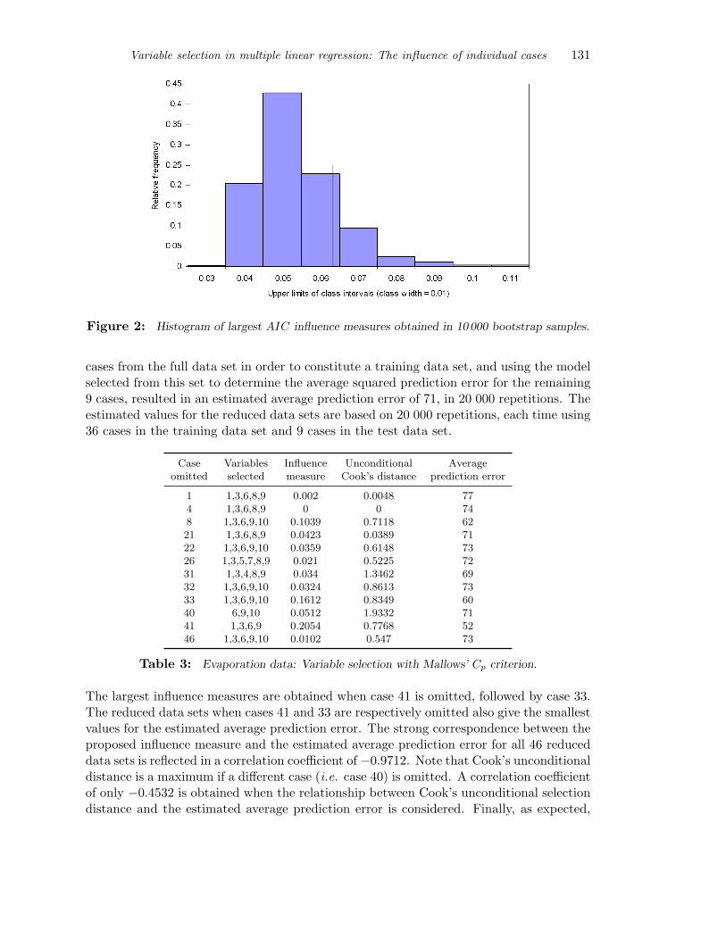
Figure 2: Histogram of largest AIC influence measures obtained in 10 000 bootstrap samples.
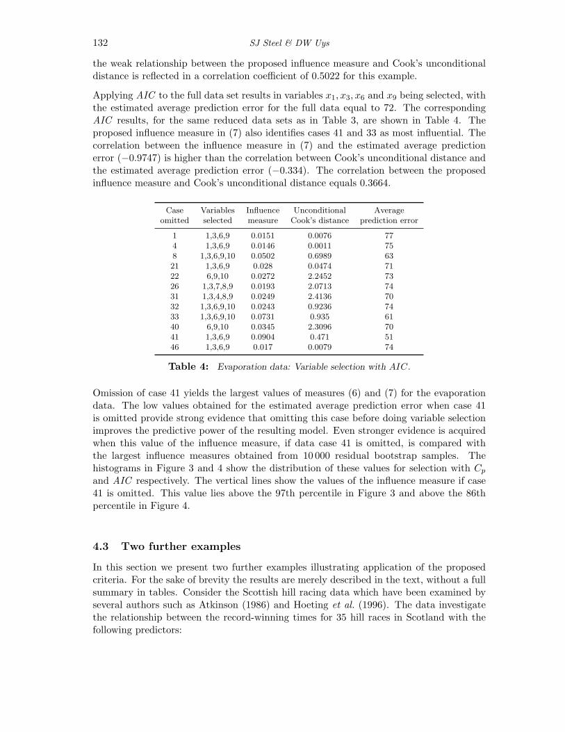
cases from the full data set in order to constitute a training data set, and using the modelselected from this set to determine the average squared prediction error for the remaining9 cases, resulted in an estimated average prediction error of 71, in 20 000 repetitions. Theestimated values for the reduced data sets are based on 20 000 repetitions, each time using36 cases in the training data set and 9 cases in the test data set.
Case Variables Influence Unconditional Averageomitted selected measure Cook’s distance prediction error
1 1,3,6,8,9 0.002 0.0048 774 1,3,6,8,9 0 0 748 1,3,6,9,10 0.1039 0.7118 6221 1,3,6,8,9 0.0423 0.0389 7122 1,3,6,9,10 0.0359 0.6148 7326 1,3,5,7,8,9 0.021 0.5225 7231 1,3,4,8,9 0.034 1.3462 6932 1,3,6,9,10 0.0324 0.8613 7333 1,3,6,9,10 0.1612 0.8349 6040 6,9,10 0.0512 1.9332 7141 1,3,6,9 0.2054 0.7768 5246 1,3,6,9,10 0.0102 0.547 73
Table 3: Evaporation data: Variable selection with Mallows’ Cp criterion.
The largest influence measures are obtained when case 41 is omitted, followed by case 33.The reduced data sets when cases 41 and 33 are respectively omitted also give the smallestvalues for the estimated average prediction error. The strong correspondence between theproposed influence measure and the estimated average prediction error for all 46 reduceddata sets is reflected in a correlation coefficient of −0.9712. Note that Cook’s unconditionaldistance is a maximum if a different case (i.e. case 40) is omitted. A correlation coefficientof only −0.4532 is obtained when the relationship between Cook’s unconditional selectiondistance and the estimated average prediction error is considered. Finally, as expected,
132 SJ Steel & DW Uys
the weak relationship between the proposed influence measure and Cook’s unconditionaldistance is reflected in a correlation coefficient of 0.5022 for this example.
Applying AIC to the full data set results in variables x1, x3, x6 and x9 being selected, withthe estimated average prediction error for the full data equal to 72. The correspondingAIC results, for the same reduced data sets as in Table 3, are shown in Table 4. Theproposed influence measure in (7) also identifies cases 41 and 33 as most influential. Thecorrelation between the influence measure in (7) and the estimated average predictionerror (−0.9747) is higher than the correlation between Cook’s unconditional distance andthe estimated average prediction error (−0.334). The correlation between the proposedinfluence measure and Cook’s unconditional distance equals 0.3664.
Case Variables Influence Unconditional Averageomitted selected measure Cook’s distance prediction error
1 1,3,6,9 0.0151 0.0076 774 1,3,6,9 0.0146 0.0011 758 1,3,6,9,10 0.0502 0.6989 6321 1,3,6,9 0.028 0.0474 7122 6,9,10 0.0272 2.2452 7326 1,3,7,8,9 0.0193 2.0713 7431 1,3,4,8,9 0.0249 2.4136 7032 1,3,6,9,10 0.0243 0.9236 7433 1,3,6,9,10 0.0731 0.935 6140 6,9,10 0.0345 2.3096 7041 1,3,6,9 0.0904 0.471 5146 1,3,6,9 0.017 0.0079 74
Table 4: Evaporation data: Variable selection with AIC.
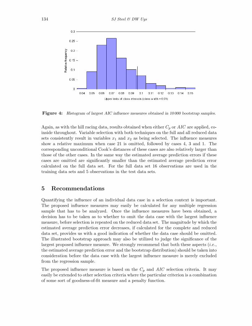
Omission of case 41 yields the largest values of measures (6) and (7) for the evaporationdata. The low values obtained for the estimated average prediction error when case 41is omitted provide strong evidence that omitting this case before doing variable selectionimproves the predictive power of the resulting model. Even stronger evidence is acquiredwhen this value of the influence measure, if data case 41 is omitted, is compared withthe largest influence measures obtained from 10 000 residual bootstrap samples. Thehistograms in Figure 3 and 4 show the distribution of these values for selection with Cp
and AIC respectively. The vertical lines show the values of the influence measure if case41 is omitted. This value lies above the 97th percentile in Figure 3 and above the 86thpercentile in Figure 4.
4.3 Two further examples
In this section we present two further examples illustrating application of the proposedcriteria. For the sake of brevity the results are merely described in the text, without a fullsummary in tables. Consider the Scottish hill racing data which have been examined byseveral authors such as Atkinson (1986) and Hoeting et al. (1996). The data investigatethe relationship between the record-winning times for 35 hill races in Scotland with thefollowing predictors:

Variable selection in multiple linear regression: The influence of individual cases 133
Figure 3: Histogram of largest Cp influence measures in 10 000 bootstrap samples.
x1 : distance covered in miles; andx2 : elevation climbed during the race.
According to Atkinson (1986) the data contain a known error: observation 18 should be18 minutes rather than 78 minutes. Here we specifically use the data set containing theerror in order to evaluate the performance of the proposed influence measures in (6) and(7). Throughout, the results obtained when either Cp or AIC are applied to the dataare very similar. Both variables are selected if the two selection techniques are applied tothe full data set. The one-at-a-time omission of case 7 or 11 leads to variable x1 beingselected. For all the other reduced data sets the same variables as in the full data set areselected.
The largest influence measures in (6) and (7) are obtained when data case 18 is omitted,followed by cases 11 and 7. The influence measures for these cases (especially case 18)are significantly larger than when other cases are omitted. Cook’s unconditional distancereaches a maximum when case 7 is omitted, with also relatively large values when cases 11and 18 are omitted. There is a sharp reduction in the estimated average prediction errorwhen case 18 is omitted. The estimated average prediction error for the reduced data setswithout cases 11 and 7 are also significantly smaller than that of the full data set. For thefull data set 28 observations are used in the training data sets and 7 observations in thetest data sets.
Finally, consider the stack loss data which also have been examined by several authors(Brownlee, 1965; Atkinson, 1985; Hoeting et al., 1996). The data investigate the rela-tionship between the percentage of unconverted ammonia that escapes from a plant in 21days, and the following three explanatory variables:
x1 : air flow that measures the rate of operation of the plant;x2 : inlet temperature of cooling water circulating through coils in the tower; andx3 : value proportional to the concentration of acid in the tower.
134 SJ Steel & DW Uys
Figure 4: Histogram of largest AIC influence measures obtained in 10 000 bootstrap samples.
Again, as with the hill racing data, results obtained when either Cp or AIC are applied, co-inside throughout. Variable selection with both techniques on the full and all reduced datasets consistently result in variables x1 and x2 as being selected. The influence measuresshow a relative maximum when case 21 is omitted, followed by cases 4, 3 and 1. Thecorresponding unconditional Cook’s distances of these cases are also relatively larger thanthose of the other cases. In the same way the estimated average prediction errors if thesecases are omitted are significantly smaller than the estimated average prediction errorcalculated on the full data set. For the full data set 16 observations are used in thetraining data sets and 5 observations in the test data sets.
5 Recommendations
Quantifying the influence of an individual data case in a selection context is important.The proposed influence measures may easily be calculated for any multiple regressionsample that has to be analyzed. Once the influence measures have been obtained, adecision has to be taken as to whether to omit the data case with the largest influencemeasure, before selection is repeated on the reduced data set. The magnitude by which theestimated average prediction error decreases, if calculated for the complete and reduceddata set, provides us with a good indication of whether the data case should be omitted.The illustrated bootstrap approach may also be utilized to judge the significance of thelargest proposed influence measure. We strongly recommend that both these aspects (i.e.,the estimated average prediction error and the bootstrap distribution) should be taken intoconsideration before the data case with the largest influence measure is merely excludedfrom the regression sample.
The proposed influence measure is based on the Cp and AIC selection criteria. It mayeasily be extended to other selection criteria where the particular criterion is a combinationof some sort of goodness-of-fit measure and a penalty function.
Variable selection in multiple linear regression: The influence of individual cases 135
Since omission of individual cases does not address the problems of masking and swamping,two or more cases may be omitted at a time. This approach, however, causes difficultieswith respect to computing time.
Acknowledgements
The authors would like to thank the anonymous referees whose valuable comments led toan improved version of the paper.
References
[1] Akaike H, 1973, Information theory and an extension of the maximum likelihood principle,The 2nd International Symposium on Information Theory, Akademia Kiado, Budapest, pp.267–281.
[2] Atkinson AC, 1985, Plots, transformations, and regression, Clarendon Press, Oxford.
[3] Atkinson AC, 1986, Comments on “Influential observations, high leverage points, and out-liers in linear regression, Statistical Science, 1, pp. 397–402.
[4] Belsley DA, Kuh E & Welsch RE, 1980, Regression diagnostics, Wiley, New York (NY).
[5] Breiman L, 1992, The little bootstrap and other methods for dimensionality selection inregression: X-fixed prediction error, Journal of the American Statistical Association, 87, pp.738–754.
[6] Brownlee KA, 1965, Statistical theory and methodology in science and engineering, 2nd
Edition, Wiley, New York (NY).
[7] Burnham KP & Anderson DR, 2002, Model selection and multi-model inference, Springer,New York (NY).
[8] Cook RD, 1977, Detection of influential observations in linear regression, Technometrics,19, pp. 15–18.
[9] Cook RD, 1986, Assessment of local influence, Journal of the Royal Statistical Society, SeriesB, 48, pp. 133–169.
[10] Choongrak K & Hwang S, 2000, Influential subsets on the variable selection, Communi-cations in Statistics: Theory and Methods, 29, pp. 335–347.
[11] Efron B & Tibshirani RJ, 1993, An introduction to the bootstrap, Chapman and Hall, NewYork (NY).
[12] Freund RJ, 1979, Multicollinearity etc.: Some “new” examples, Proceedings of the StatisticalComputing Section, American Statistical Association, pp. 111–112.
[13] Hoeting J, Raftery AE & Madigan D, 1996, A method for simultaneous variable selec-tion and outlier identification in linear regression, Computational Statistics and Data Anal-ysis, 22, pp. 251–270.
[14] Kundu D & Murali G, 1996, Model selection in linear regression, Computational Statisticsand Data Analysis, 22, pp. 461–469.

136 SJ Steel & DW Uys
[15] Leger C & altman N, 1993, Assessing influence in variable selection problems, Journal ofthe American Statistical Association, 88, pp. 547–556.
[16] Liu H, Weiss RE, Jennrich RI & Wegner NS, 1999, PRESS model selection in repeatedmeasures data, Computational Statistics and Data Analysis, 30, pp. 169–184.
[17] Mallows CL, 1973, Some comments on Cp, Technometrics, 15, pp. 661–675.
[18] Mallows CL, 1995, More comments on Cp, Technometrics, 37, pp. 362–372.
[19] Miller AJ, 2002, Subset selection in regression, 2nd Edition, Chapman and Hall, London.
[20] Murtaugh PA, 1998, Methods of variable selection in regression modeling, Communicationsin Statistics: Simulation and Computation, 27, pp. 711–734.
[21] Venter JH & Snyman JLJ, 1997, Linear model selection based on risk estimation, Annalsof the Institute of Statistical Mathematics, 49, pp. 321–340.
[22] Weisberg S, 2005, Applied linear regression, 3rd Edition, Wiley, New York (NY).