variability of the wind stress curl over the north pacific

JOURNAL OF GEOPHYSICAL RESEARCH, VOL. 96, NO. C10, PAGES 18,361-18,379, OCTOBER 15, 1991

Variability of the Wind Stress Curl Over the North Pacific' Implications for the Oceanic Response

1 ALAN D. CHAVE

AT&T Bell Laboratories, Murray Hill, New Jersey

DOUGLAS S. LUTHER AND JEAN H. FILLOUX

Scripps Institution of Oceanography, La Jolla, California

The subinertial frequency-wavenumber structure and spatial coherence of wind stress curl, and their spatial and temporal variability, are described with the emphasis on characteristics which affect the ocean's response to the wind stress curl forcing function. Wind stress curl over the North Pacific between 25 ø and 60øN was computed for 3 years (1985-1988) from the Fleet Numerical Oceanography Center wind product. The range from winter peak to summer trough for the mean and variance are typically a factor of 3-4 and = 10 respectively, with superimposed interannual changes of up to a factor of 2. Power spectra vary seasonally and interannually in an essentially frequency-independent manner that is consistent with the curl variance. However, the spectrum over the period band 5-100 days often fails a statistical test for whiteness at the 95% level. Zonal and meridional wavenumber spectra were estimated for 13 sites distributed around the central-eastern North Pacific using the maximum likelihood method. Directional trends with frequency are comparable to those from earlier studies if 3-year-long data segments are analyzed, with approximate wavenumber symmetry except for the zonal term at mid-latitudes for periods shorter than 10 days, where eastward propagation is dominant. However, spectra for shorter data sections sometimes display eastward and westward excursions which are only weakly similar over distances of =1000 km and essentially dissimilar over longer separations. The spatial correlation structure of wind stress curl is shown typically to have a main lobe of =1000 km and multiple intercorrelation lobes separated by > 2000 km. The strength and location of the intercorrelation peaks vary slowly with time. These results suggest that curl behavior is more complex than was previously believed, that the use of long-term averages of or simple parameterizations for the frequency-wavenumber spectrum of wind stress curl in model studies may be unrealistic, and that more attention to actual curl characteristics at the time oceanic measurements are collected will be required to reconcile models with observations.

1. INTRODUCTION

Much of the barotropic variability of the deep ocean at periods of days to months is directly, atmospherically forced except near regions dominated by the instabilities of strong mean currents and the concomitant radiation of mesoscale eddies. This assertion is

supported by several model studies which predict coherence between oceanic and atmospheric variables that is either local [Willebrand et al., 1980; Muller and Frankignoul, 1981] or nonlocal [Brink, 1989; Satnelson, 1989], depending on topography, the oceanic variable under consideration, and the frequency and vector wavenumber of the forcing which dictate whether an evanescent or free Rossby wave response is possible. In addition, observational evidence is accumulating for both local and nonlocal coherence of ocean currents and the wind forcing in areas of weak eddy variability [Niiler and Koblinsky, 1985; Koblinsky et al., 1989; Brink, 1989; Luther et al., 1990; Satnelson, 1990].

Philander [1978] and Frankignoul and Muller [1979] showed that the dominant atmospheric forcing variable for extratropical latitudes is the vertical component of wind stress curl (hereinafter

I Now at Woods Hole Oceanographic Institution, Woods Hole, Mas- sachusetts.

Copyright 1991 by the American Geophysical Union.

Paper number 91JC02152. 0148-0227/91/91JC-02152505.00

simply curl) at periods longer than a day and for horizontal scales larger than a few hundred kilometers. In fact, the model studies cited above were all curl forced. The numerical result of Wille-

brand et al. [1980] employed geostrophic winds computed from surface air pressure maps as the input, while the remaining models are based on the stochastic approximation with the characteristics of curl specified by an analytic frequency-wavenumber spectrum. In general, the results are sensitive to both the frequency and the wavenumber content of curl. This is especially true for the zonal wavenumber spectrum because of the strong influence which the amount of power in westward wavenumbers has on the excitation of free Rossby waves. Thus, a good description of the spatial and temporal variability of curl is essential both for the generation of realistic models and for the interpretation of oceanic data.

A number of attempts have been made to estimate the spatial and temporal scales of the winds on a global or hemispheric basis outside the surface boundary layer [e.g., Willson, 1975]. Together with some theoretical arguments, these results were used by Frankignoul and Muller [1979] to construct surface frequency- wavenumber spectra of the atmospheric variables at mid-latitudes for periods of days to months. However, such estimates lack horizontal resolution of small-scale wind features, which has important consequences for computation of curl, and in any case are not based on measurements of the winds in the surface boundary layer which are most relevant to the oceanographer. Willebrand [ 1978] inferred the frequency-wavenumber characteristics of the geostrophic winds from synoptic surface pressure data collected over the oceans during 1973-1976. His results suggest a symmetric

18,361

18,362 CHAVE et al.: WIND STRESS CURL VARIABILITY

zonal wavenumber spectrum for curl at periods longer than =10 days at mid-latitudes with a corresponding white frequency spectrum. At shorter periods, eastward traveling cyclones and anticy- clones are dominant, yielding an increasingly asymmetric zonal wavenumber spectrum for curl as period decreases and introduc- ing redness into the frequency spectrum. South of =35 ø and north of =50 ø the short period asymmetry disappears. The meridional wavenumber spectrum of curl is approximately symmetric with a slight northward bias at all periods. Finally, MacVeigh et al. [1987] computed curl from 4 years of European Center for Medium Range Weather Forecast (ECMWF) product to examine both large-scale spatial variability and gross wavenumber properties excluding directionality, showing some agreement with Willebrand's result.

It appears that most of the available information on the frequency-wavenumber structure of curl at periods of days to months is summarized by the work of Willebrand [1978] and Frankignoul and Muller [1979]. However, a number of recent investigations of monthly mean oceanic wind data have appeared in the literature. These studies are typically concerned with basin scale spatial patterns and the annual or semiannual components based on empirical orthogonal function analysis covering the North Atlantic [e.g., Ehret and O'Brien, 1989] and the North Pacific [Rienecker and Ehret, 1988]. Only Gallegos-Garcia et al. [ 1981 ] estimated curl wavenumber properties from monthly mean data (with results that are somewhat discordant with those of MacVeigh et al. [1987]). However, these studies shed no light on the behavior of curl at periods shorter than two months.

The purpose of this paper is to begin to fill this void in the literature by examining the spatial and temporal characteristics of curl over the North Pacific during 1985-1988. The wind data are obtained from the Fleet Numerical Oceanography Center (FNOC) data product, which is more complete than the measurements available in earlier short-period studies. The primary motivation for the work is a critical examination of the variability on time scales shorter than the seasonal, where the oceanic response may either be evanescent or resonant depending on the wavenumber characteristics of the forcing. A secondary goal is to serve as an aid for the interpretation of an array of seafloor pressure and barotropic current data collected during the Barotropic Electromag- netic and Pressure Experiment (BEMPEX), which was designed to study atmospheric forcing of the deep ocean [Luther et al., 1987]. The BEMPEX data have already been found to be strongly coherent with local and/or nonlocal FNOC surface air pressure, wind stress, and wind stress curl [Luther et al., 1990; A.D. Chave et al., The Barotropic Electromagnetic and Pressure Experiment, 1, Barotropic current response to atmospheric forcing, submitted to Journal of Geophysical Research, 1991, hereinafter referred to as Chave et al. ( 1991)].

In the next section, the FNOC data and estimates of curl derived from them are outlined. Section 3 constitutes an exami-

nation of the mean and variances of the curl field over the North

Pacific for various averaging times with the purpose of both emphasizing the seasonal range and relating the results to the dominant atmospheric processes which control North Pacific climate. Section 4 discusses the frequency spectrum of curl in the period range of a few days to a few months, showing that whiteness at periods greater than 5-10 days is at best approximate. A weak concentration of variance near 30 days period observed throughout the central-eastern North Pacific is also described. Section 5 presents maximum likelihood zonal and meridional wavenumber spectra for various averaging intervals which suggest that significant temporal and spatial curl inhomogeneity is

present. When 6-month data sections are analyzed, eastward or westward propagation of curl is noted at different times with no obvious seasonal dependence; for longer time series these motions average away to produce wider apparent wavenumber peak widths with no preferred propagation direction. Section 6 exam- ines the spatial correlation structure of curl over the North Pacific, finding that small-scale (= 1000 km) coherent patches separated by larger (_•2000 km) distances appear to be ubiquitous, so that simple unimodal parameterizations of curl's autocorrelation are unrealistic. The final section of the paper is a discussion of the consequences of these analyses for modeling atmospherically-forced oceanic motions at subinertial periods out to 100 days.

2. THE WIND OBSERVATIONS

The raw data used in this study consist of 3-year sequences of the vector wind velocity at 405 locations distributed over the North Pacific and obtained from the Fleet Numerical Oceanogra- phy Center. The FNOC winds are calculated iteratively from surface atmospheric pressure data blended with wind observations using a combination of objective analysis and prognosis which includes ageostrophic effects and an adjustment for frictional effects in the surface boundary layer. An early version of the FNOC algorithm is described by Lewis and Grayson [1972]. The FNOC product is reported every 6 hours on a polar stereographic grid at an altitude of 19.5 m. The time series were nearly complete for the interval July 1985 through June 1988, with missing data constituting less than 1% of the total and covering only brief intervals which could easily be linearly interpolated. The sample spacing is uniform on a stereographic grid and hence uneven in geographic coordinates, but is typically 340 km near the center of the region of interest (40øN, 162øW) with smaller (larger) values to the north (south).

Because of the complex data assimilation method used to obtain the FNOC product, it is difficult to quantify the accuracy or smoothing scales of the resulting wind estimates. Ship observations of air pressure, wind velocity, and wind direction are a major input for the FNOC product, and recent studies indicate that significant errors occur in such data with distressing frequency [e.g., Wilkerson and Earle, 1990]. However, the analysis procedure is designed to correct for bad data in a self-consistent manner, and the relative success of this approach is attested to by a number of intercomparisons between the FNOC winds and either other data products or actual measurements. For example, Friehe and Pazan [1978] found good agreement between NOAA buoy data and the FNOC product in the North Pacific near 35øN, 155øW. De Young and Tang [1989] contrasted the FNOC winds with measurements from an oil platform on the Grand Banks, finding high correlations (=0.9) at periods longer than 2 days and measurable discrepancies in direction at wind speeds under 10 m s-• and for the summer months. Brink [1989] compared measured winds obtained with moored buoys in the subtropical North Atlantic during the Frontal Air-Sea Interaction Experiment (FASINEX) with three data products: the FNOC values, the NOAA Analysis of the Tropical Ocean Lower Layer (ATOLL) winds, and a simpler geostrophic estimate. Of the three, the FNOC winds were the most highly correlated with the measured winds (192> 0.9) and appeared to reproduce them with acceptable accuracy. Halliwell and Cornilion [ 1990] performed a more thor- ough analysis of the in situ, FNOC, and ATOLL winds during FASINEX and found that measured averages were best repro- duced by the FNOC values. However, Pazan et al. [1982] found poor agreement of the FNOC product with measured winds in the

CHAVE et al.: WIND STRESS CURL VARIABILITY 18,363

equatorial Pacific where actual observations are very limited. Thus, it appears that the FNOC product yields usable estimates of surface winds over the ocean at periods longer than a few days and when wind velocities are moderate to large, especially in regions where ship traffic is relatively dense, such as the mid- latitude Noah Pacific.

The 19.5 m FNOC winds were iteratively transformed to wind stress at a height of 10 m using Monin-Obukhov similarity theory and a velocity-dependent neutral drag coefficient under the assumption of constant air density. No directional correction for boundary layer rotation was applied. The drag coefficient formu- lation is comparable to the standard Large and Pond [ 1981 ] value for wind velocities over 3 m s -I , but has a constant plus inverse velocity relationship in weak winds as discussed by Trenberth et al. [ 1989].

The wind stress curl was computed using a two-dimensional centered finite difference operator on a sphere. Consider a function f(qb,X,), where qb is longitude and X, is latitude, and expand it in a Taylor series for small increments œ and 15

f(qb+œ,•,+8) = f(qb,•,) + A'Vlf(qb,•,) +

«(A'Vl)2f(qb,•,) + ... (•)

where

A= [aœcosX,, aiS] and the surface gradient operator is given by

V• = acosX, *' a

with a as the radius of the Earth. To determine the first and

second derivatives in (1), five equations and hence six data are needed, while the FNOC grid yields only five data if a cross centered on the point of interest is used. An additional datum could be obtained by sampling one of the four comers of the square cir- cumscribing the cross, but there is no a priori reason to choose one over the others. For this reason, the derivatives were esti-

mated by using each of the four comers in turn and averaging the

3. MEAN AND VARIANCE OF CURL

Figure 1 shows the curl mean for the 3-year interval July 1985 through June 1988. In the sequel, all contour maps will be shown on the original uniform FNOC polar stereographic grid to avoid interpolation error, with selected latitude and longitude lines and outlines of the continents included as an aid to the eye. Specific grid locations will be referred to by a four digit number where the first (last) two digits correspond to the meridional (zonal) indices on the axes of the figures. Both the spatial patterns and the magnitudes of the curl mean in Figure 1 are similar to the recent com- pilation of Harrison [1989], which is not surprising given that he used essentially the same drag coefficient as in the present study. The major exception occurs near the west coast of North America where Figure 1 shows a southward deflection of the zero contour; this is the result of a pervasive high-pressure cell over the south- western U.S. land mass whose influence has been included in the

present data. Slightly better agreement is seen between Figure 1 and the mean computed from the Comprehensive Ocean- Atmosphere Data Set (COADS) by Rienecker and Ehret [1988], especially near North America. Figure 2 shows the variance for the same 3-year time interval. The variance or total power is largest immediately south of the Aleutian Islands, reflecting the influence of the Aleutian low to the north and the subtropical high to the southeast on average storm tracks. Note that the variance contours shown in Figure 2 are at least an order of magnitude larger than those given by Rienecker and Ehret; this is simply due to the use of 6-hourly data in this study as opposed to monthly averages for their result.

Figure 3 compares the 3-year averaged summer (July-September), fall (October-December), winter (January-March), and spring (April-June) variances for curl. The range exceeds a decade at mid-latitudes with the largest values in winter and the smallest ones in summer, but with the peak located somewhere in the middle of the basin sou th of the Aleutian Islands. The variance reflects the climatology of the North Pacific which is dominated by the Aleutian low during winter and

results to minimize possible bias errors. The standard error com-

puted from the four derivative estimates was typically less than one tenth of the mean. The vertical component of the curl of the .• wind stress • in spherical coordinates follows from • • "I•- • Vx•'• = 1 I3 )1 a cosX, ,'rx - 3x(cosX, •:, (2) • 20 -

a ndyieldsestimatesat3251ocationsafterexcludingtheouterbor- •_• l• / "••/ • •///•0ø der of the original grid. This approach provides explicit control 1 • / of the derivative error (unlike with two dimensional polynomial approximations), does not require a final rotation to geographic .• 1 6 coordinates, and does not ignore the mixed derivative in the second order term as would a more conventional finite difference • ! 4 approach.

It should be noted that the application of spatial derivative operators to a smoothed atmospheric variable results in truncation of high wavenumber components and possible reduction of the wavenumber bandwidth [Willebrand, 1978]. This effect could be severe for estimates of curl but is difficult to quantify on account of the spatially variable and data-dependent smoothing inherent to the FNOC product. Based on algorithmic descriptions provided by Lewis and Grayson [1972], the smoothing scale varies from 300 to 850 km. Consequently, inferences about the properties of curl at wavelengths smaller than roughly 500 km must be regarded as of questionable reliability.

40 B5 30 25 20

Zonal Grid Point

Fig. 1. Contour map of time-averaged curl for the interval July 1985 through June 1988 over the North Pacific Ocean shown on the FNOC polar stereographic grid. Selected latitude and longitude lines and the outlines of North America, the Kamchatka Peninsula, Sakhalin Island, and Japan are shown as aids to the eye. The axes are labeled with the FNOC meridional and zonal grid points. The contours have units of dynes per cubic centimeter scaled by 10 9 .


• 24 ' c.•

- ' I • - ,._ /5 0 ø

-. • ß 500

[

_ \

I I I 0 C

40 35 30 25 20

Zon•z• Cr•;d Point

Fig. 2. Contour map of curl variance for the interval July 1985 through June 1988 over the North Pacific Ocean shown on the FNOC polar stereographic grid. The contours have units of dynes 2 cm -6 scaled by 1018 Otherwise plotted as in Figure 1.

the subtropical high during summer [Terada and Hanzawa, 1984]. >From late fall through winter, the low is centered near 50øN, 175øE and extends across most of the basin; it is particularly intense because of the frequent southeastward passage of depres- sions from the Bering Sea and Asia. At the same time, the subtropical high shrinks and is pushed well to the southeast, being centered near 30øN, 140øW. The effect of the low on storm

tracks and cyclogenesis is reflected in the fall and winter curl variance maps of Figure 3. By contrast, in the summer the subtropical high covers most of the North Pacific and is centered near 40øN, 150øW with the Aleutian low pushed well into polar regions. This results in a substantial reduction in storm frequency and intensity, and a marked decrease in the curl variance. The fall and spring variances are transitional, respectively reflecting the rapid growth of the low- and high- pressure systems. Note the differences between the seasonal averages of Figure 3 and the 3- year values in Figure 2. The latter most closely resemble the fall-winter values, which is not surprising given the nonrobust nature of the variance statistic.

Comparable seasonal changes in the curl mean are also observed. During the summer, the zero curl contour extends from the coast of Alaska at 55øN to 35øN in the west half of the basin.

• 24

• 22

• 20

½ 24 'to

r• 22

ß • 20

18

•16

.• 14

. • _ 50 ø . . •

I • l?Qø ,.. I 1140 c

40 35 30 25 20

Zonal O•{d Point

½ 24

ß • 20

18

••4

•12

40 35

fall 7d •. /50ø,,.

170 ø ,,, ... • \ 140 ½

30 25 20

tv•nter - v

40 35

170 ø .... , \ 14oø•

'• 24

r• 22

• 20

_.

_....? 300 ß 170 ø \140

30 25 20 40 35 30 25 20 Zo•a[ G?•ct Po{•zt Zor•c•L Gr•,ct Po•;•zt

Fig. 3. Contour maps of seasonal curl variance for the interval July 1985 through June 1988 over the North Pacific Ocean shown on the FNOC polar stereographic grid. Each panel gives the variance for 3 months of the year averaged over 3 years, with summer, fall, winter, and spring beginning at the start of July, October, January, and April respectively. The contours have units of dyn 2

- 18 cm 6 scaled by 10 . Otherwise plotted as in Figure 1.


2328 2027

•- f6 •10-

10-•? -------- I I I IllIll I I I 111111 I I I 111111 I I I II1111 I

10-3 10-2 10-½ 10 o

Frequency (d-•)

10-•?

_

_

-= i i ii11111 i i i iiiiii I i i iiii1! I I I Iiiiii ! i

10-3 10-,e 10-• 10 0

Frequency (d- •)

1830 1330

10-•3

I

10

½ -•5

•0-•?

_=_ 95%

_

111111 i i i IIIIii i i i IIII11 i i i 11!111 I i

10-3 10-2 10-½ 10 o

Frequency (d- •)

10-•'3

i

½ 10

• -½5 •10

•' -16 •10

10-•?

== 95

_

_

• I I I III111 I I I IIIIII I I I IIII1,1 I I IIIII11 ..... I I

10 -3 10 -2 1 O- ½ 10 ø

Frequency (d- •)

Fig. 4. Multiple window power spectra of wind stress curl for the interval July 1985 through June 1988 at the FNOC sites as labeled with their meridional and zonal grid point numbers. The units of frequency are cpd, while power is in dyn 2 cm -6 per cpd. The time-bandwidth of the estimate is 4, corresponding to a spectral bandwidth of 0.0072 cpd, and each frequency has -- 14 degrees of freedom, yielding a double-sided 95% confidence interval of (0.54,2.48) times the estimated power for Gaussian data. The bandwidth of the estimate centered on a 30 day period is delimited by the short horizontal bar. Note the approximately white back- groun d for periods longer than a few days with weak peaks superimposed, especially at 30 days.

Positive curl is restricted to the environs of the Aleutian chain and

north. By contrast, in the winter the zero curl contour lies at about 35øN in the center of the basin with northward curvature at

the east and west ends, and the region of positive curl dominates most of the mid-latitude ocean. The winter curl peak value is at least 4 times the summer one. The fall and spring months reflect the transition between these extremes. The 3-yea.r average of Fig- ure 1 is intermediate between the seasonal extremes.

The interval July •986 through June 1987 (hereinafter year 2 and nearly coincident with the BEMPEX experiment) also presents some contrasts with the two surrounding years. During the first 9 months the mean is typically 50% larger and the variance is double the 3-year values, especially near the middle of the Pacific basin, while during the spring of 1987 the differences decrease somewhat except in the Gulf of Alaska. Year 1 (July 1985 through June 1986) is only slightly weaker than year 2 in all seasons, while year 3 (July 1987 through June 1988) presents uni- formly .weaker curl (by about a factor of 2) throughout the mid-

latitude North Pacific. Thus, year 2 stands out as being more energetic through most of the seasons. Interestingly, a weak E1 Nin0 event occurred in 1986-1987 [Kousky and Leetmaa, 1989], which could' haye affected the climate over the mid-latitude North Pacific in late 1987 to early 1988 during year 3.

It shou. ld be noted that long-term averages such as those of Fig- ures 1 and 2 may be of limited value in inferring the magnitude of the ocean's transient response •to atmospheric forcing in any given season or year. It is clear that seasonal variability of curl is significant, but also that interannual changes cannot be ignored.

4. FREQUENCY SPECTRA OF CURL

Frequency spectra of curl appear qualitatively to be white for periods longer than a few days, with some additional, location- specific differences being evident. The level of the spectrum varies with both position and season in an essentially frequency- independent manner. For a given latitude, the power is largest


near the middle of the basin and weaker by a factor of 2-4 at the edges, while for a given longitude the power decreases by over a decade from 55øN to 30øN. The seasonal range at a single location and frequency is typically a factor of 2-4, with larger excursions evident at more northern latitudes.

However, inspection of high-resolution spectra reveals some real features superimposed on the white background which deserve closer attention. Figure 4 shows power spectra for four locations estimated with the multiple prolate window expansion of Thomson [ 1982] using 3 years of curl data. A multiple window spectrum is computed by first generating a set of orthogonal data windows which are optimal in a minimum spectral leakage sense and which depend explicitly on the time-bandwidth product (resolution bandwidth times data series length). These windows are each applied to the data as tapers prior to Fourier transformation, and since the windows are orthogonal, the raw estimates are approximately independent. The raw spectra are combined using a set of weigh,ts chosen to minimize broadband bias (spectral leakage). The resulting spectrum is effectively the convolution of the unknowable true spectrum with a rectangular frequency domain window of width specified by the chosen time-bandwidth product.

a necessary and sufficient check for spectral whiteness. The M statistic is

M = Nlog [• viSi] + •v/log[St] (3) i=1 i=1

where N = • v i and v i is the degrees of freedom for the spectral estimate S i at the i-th frequency. For small samples, Bartlett showed that M/C, where

1 [• 1 1] (4) C = 1 + 3(k-l) i=•vi N

is approximately distributed as Z 2 for k-1 degrees of freedom. Table 1 shows the results of this test applied to 13 spectra computed from 3-year curl time series. A period range of 5-100 days was used to avoid any bias from the weak annual and semiannual components and from the short-period roll-off. The result is not overly sensitive to the choice of short-period cutoff over the 5-10 day interval. To ensure data independence, the spectral power at frequencies separated by more than the resolution bandwidth was used. For each site, estimates at 25 frequencies were pooled, and

This procedure results in an increase in statistical efficiency com- since Z224(0.95)=36.4, it is clear that seven of the M values pared with conventional band-averaging with complete control of exceed the threshold, and hence the corresponding spectral esti- spectral leakage. mates are not drawn from a homogeneous variance population at

Rienecker and Ehret [1988] fit deterministic annual and semiannual terms to 20 years of curl data, and found that they typically account for less than 10% of the variance in the central-eastern

North Pacific. Using an F test for deterministic components to a spectrum devised by Thomson [1982] yields a significant annual term at only a single site in the Gulf of Alaska (2328 at 55øN, 146øW) and no significant semiannual terms. The remaining sites, as well as many others which were examined, show only the slight variance enhancement at periods longer than --100 days seen in Figure 4, indicative of the weakness of the semiannual and annual components. Weak spectral peaks do appear at shorter periods for many eastern North Pacific sites, most commonly near 30 days as typified by sites 2027 (45øN, 147øW), 1830 (41øN, 162øW), and 1330 (27øN, 164øW) in Figure 4. This peak is usu- ally significant at about the 80% level, and its shape reflects the bandwidth of the spectral estimate rather than of the underlying physical process. The 30-day peak is very common throughout the area, and is not removed when spectra are computed using the robust methods of Chave et al. [ 1987], suggesting that it is not an artifact of nonstationarity in the curl time series. Note also that the spectral slope for location 2328 in the Gulf of Alaska is --f- for periods of 3-100 days, and that a white background is not apparent for location 1330. The latter is common for curl at latitudes below --35øN, as is a weaker high-frequency roll-off beginning at longer periods than for higher latitudes. The spectra typically display flattening of the slope above 1 cpd, suggesting a noise floor possibly due to limitations of the FNOC product.

Figure 5 shows similar multiple window spectra covering the same sites as in Figure 4 for only year 2. Since the time series length is reduced by a factor of 3, the bandwidth of the estimate rises proportionately, and the behavior at periods longer than --90 days is obscured by the weak annual and semiannual terms. However, increased variance is evident at 30 days at all four sites, and the variance is enhanced at many eastern North Pacific locations compared with the 3-year average.

It appears that the usual assumption that the spectrum of curl is white at periods longer than a few days is only approximate. In fact, Bartlett's M test [Bartlett, 1937] to check a population of independent variance estimates for homogeneity can be applied as

the 95% confidence level. At the 90% confidence level

(Z2•4 (0.90)= 33.2), an additional two sites fail the test. There is a definite bias toward the upper end of the Z 2 range for all save one of the sites reported in the table, and the values of M/C do not scatter around the expected mean of 24. Note that if the spectra were white, then only one site might be expected to fail the test at the 90% confidence level. Of the four spectra shown in Figure 4, only site 1830 passes the whiteness test, as appears visually rea- sonable. For the remaining locations, the M test result is consistent with visual impressions. The conclusion that curl spectra are often not formally white must be tempered with caution because the Bartlett test is sensitive to nonstationarity. However, it is not clear that temporal nonstationarity immediately translates into frequency-dependent nonstationarity of the spectrum, although it will certainly reduce the equivalent degrees of freedom. The Bartlett test is also conservative in the sense that the data are not

ranked; a trend (such as a generally nonzero spectral slope) will affect the outcome only to the extent that it alters the variance range and not by ordering the data.

It is believed that the flatness of the low-frequency curl spectrum is due to dominance by a white noise extension of a high- frequency process with a short correlation time scale, in this case weather fluctuations [Frankignoul and Muller, 1979]. However, real low-frequency atmospheric fluctuations may also be significant, accounting for the departures from whiteness seen in Figures 4 and 5 and detected by the Bartlett M test. In particular, the weak 30 day peak probably represents a real low-frequency process. This may be important for understanding atmospheric forcing of the ocean. For example, enhanced power in curl over restricted frequency bands could result in an increased evanescent or free wave response, depending on both the frequency and the associated vector wavenumber characteristics.

Contour maps of power in a given frequency band are qualitatively like the variance maps of Figures 2 and 3. Since the spectrum is almost white, such maps do not display any strong frequency dependence. The seasonal variation appears like that in Figure 3 with somewhat larger ranges in the east than in the west parts of the basin. Interyear changes are also comparable to those in the simple variance. Year 2 stands out in power as compared


2328 2027

•" -f6 •10

10-•?

_

=- 95%]

--- I I I IIIIII I I I IIIII1 I I I 111111 I I IllJill I I

10 -3 ! 0 -2 ! O-• ! 0 ø

(d -

1830

10-13

o-4

•" -f6 •10

10-•?

=- 95%

_

'• I I IIIIIII I I I IIIIII I I I IllIll I I I IIIIII

10-3 10-2 10-!

Frequency (el -j )

I I

1o o

1330

10-13

10 -•4

•.. f6 •)10-

10-•?

_

_

_

_

_

-• I I i iiiiii I I i iiiiii i i i Illill I I I Illill I I

10 -a ! 0 -2 ! O-• ! 0 ø

Frequency (d -

10-13

o-4

-•5

•" -f6 •10

10-•?

== 95%

_

-• I I I IIIIII I I I IIIIII I I I IIIIII I I I IIIIII I I

10 -3 ! 0 -2 ! O-• ! 0 ø

Frequency (el- • )

Fig. 5. Multiple window power spectra of wind stress curl for the single year interval July 1986 through June 1987 at the FNOC sites as labeled. The time-bandwidth of the estimate is 4, corresponding to a spectral bandwidth of 0.022 cpd, and each frequency has --14 degrees of freedom, yielding a double-sided 95% confidence interval of (0.54,2.48) times the estimated power for Gaussian data. The bandwidth of the estimate centered on a 30 day period is delimited by the short horizontal bar. Note the stronger presence of the 30 day peak, especially at 1330, and the existence of other fine structure on the white background spectrum.

to the previous and the following years, especially in the central- eastern North Pacific.

5. WAVENUMBER SPECTRA OF CURL

The dominant atmospheric scales at mid-latitudes are a few thousand kilometers and hence only slightly smaller than the Pacific basin. Because of this large scale, conventional wavenumber estimators lack adequate resolution to infer their properties, a problem which is exacerbated by spatial heterogene- ity of power. For this reason, zonal and meridional wavenumber spectra for curl were computed using the maximum likelihood method (MLM) of Capon [1969]. Unlike conventional approaches, MLM employs a wavenumber spectral window whose shape and sidelobe structure is data-dependent and hence changes with the wavenumber in a well-defined, optimal manner. The resolution of MLM depends primarily on the incoherent noise present on the sensors and only weakly on the natural beam pattern of the array, so it is typically much better than for conventional estimators. MLM spectra were obtained for five-element

cells in the form of a cross centered on the location of interest. In

each case, the frequency spectrum was first computed using the multiple window technique, then the two dimensional wavenumber spectrum was calculated for frequencies spaced evenly in the

TABLE 1. M Test for Spectral Whiteness

Site M/C 90% 95%

1934 35.7 x

1534 25.5

2332 25.1

1830 17.5

1330 53.7 x 2328 52.0 x

1628 44.5 x

2027 47.9 x

2324 32.0

1924 36.0 x

1524 71.0 x

1720 52.6 x

2019 39.6 x


-0.4

;•-1o .

-1.,8

-1.6'

-1.8 -2.0 -2.2

s -

-0.6 0.0 0.6

3 .• -0.4 • -0.6 5 'e

7 •, '-- -0.8 10 •- *-1 0 • ß

• • -1.2

30 • •-1.4 • • -1.6

50 • • -1.8

100 • • -2.0 -2.2

E-W Wavenumber (M'm. -•)

5- 6

-0.6 0.0 0.6

E - F W ccu e rt, • wa b e •

3

5

20 • . •.•

30 •

5O

lOO

•-1o .

-1.2

-1.4

-1.6'

-1.8 -2.0 -2.2

7/86-7/87

-0.6 0.0 0.6

3 .• -0.4

? -o.s 10•- *-10 • ß

• -1.2 20

t,, • -1.4 30 • • -1.6

50

• -1.8 100 • -2.0

-2.2

E- W Wavenuwabew (M'm.- 1)

?/s ? - ?/s s

_3 s 5

10•-.

• ,20 •

30 • 50

•00

-0.6 0.0 0.6

E-W Wavenumber (Mwn. -1)

Fig. 6. Zonal wavenumber spectra for FNOC site 2328, located in the Gulf of Alaska, computed using the maximum likelihood method. The estimates encompass the time interval July 1985 through June 1988 and the three annual periods contained therein. The frequency bandwidth is constant at 0.027 cpd for all of the spectra. The wavenumber has units of cycles per megameter. Power is expressed in decibels down from the peak at each frequency at the peak meridional wavenumber. This means that larger numbers correspond to weaker power. Note the wider apparent peak width for the 3-year estimate when compared to the year 1 and 2 results.

logarithmic domain. Zonal (meridional) sections as a function of frequency are then presented at the meridional (zonal) wavenumber corresponding to the peak in power. By using different length data sections, information on the varying propagation characteristics of curl over time can be inferred. Davis and Regier [1977] have shown that MLM is an accurate method to locate the peak wavenumber but may not be the best method to estimate other properties of continuous spectra such as high-frequency slope. As a consequence, emphasis will be placed on gross wavenumber properties rather than on spectral details.

Capon and Goodman [1970] have shown that MLM spectra are Z 2 distributed with n =2(m-k + 1 ) degrees of freedom assuming that the data are approximately Gaussian, where m is the number of independent frequency estimates and k is the number of sensors. The wavenumber spectrum is ordinarily normalized by the peak value at each frequency and plotted in the logarithmic domain; for testing the significance of the peak, it is often appro-

priate to determine when the peak power is different from the power at zero wavenumber at a specified confidence level. Using the definition of a confidence interval gives

2

•p - •o = 10log x,•,; _ (5) I or/2

where •t, is the estimated peak power and •o is the estimated power at zero wavenumber, both expressed in decibels (dB). A similar test can be applied to changes in relative power between different time sections at a selected wavenumber if it is assumed

that the peak power to which the spectra have been normalized does not change. When considering significance tests in the sequel, it should be remembered that the degrees of freedom estimate is based on the assumption that the k sensors are independent. Due to the smoothed form of the FNOC product, this is only approximately correct, and hence the estimated degrees of


freedom with k = 5 will be a lower limit. At the same time, curl time series are clearly nonstationary, and hence frequency estimates computed from them will have fewer degrees of freedom than conventional wisdom would suggest. This means that significance tests should be treated as approximations that are useful for qualitative comparison of spectra frequency-by-frequency, and will not be followed rigorously in what follows.

Zonal and meridional spectra were computed for 13 locations on the FNOC grid distributed between 25øN and 55øN and east of the 180 ø meridian. Figures 6-9 show zonal wavenumber spectra at 16cations 2328, 2027, 1830, and 1330 (the same sites for which power spectra,are displayed in Figures 4-5) for the entire 3-year and individual 1-year intervals using identical resolution band- widths. The 3-year spectra have 32 nominal degrees of freedom while the annual ones have 10 nominal degrees of freedom; using (5) requires =2.3 and =4.2 dB difference of the peak from the zero wavenbmber value at 1 standard deviation for an individual esti-

mate. Comparable values may be used to assess changes between time sections.

At the northernmost site of Figure 6 (2328) there is a weak suggestion of a wider peak width in the 3-year spectrum than for individual year spectra. Comparison of the yearly spectra indi- cates that this is due to substantial interannual variation in behav-

ior; the 3-year estimate reflects the long-term variability. The 3- year spectrum appears to be nearly symmetric at all frequencies, with only weak tendencies for eastward propagation at periods shorter than 10 days and westward propagation at 10-50 days which are obscured by the width of the peak. However, the individual spectra suggest eastward propagation at periods of 6-12 days in year 1 and westward propagation at periods of 13-50 days in year 2 and 15-22 days in year 3. Other, weaker suggestions of eastward and westward propagation are also evident.

The two mid-latitude sites 2027 and 1830 (Figures 7 and 8) display a markedly stronger tendency for eastward propagation at periods shorter than 10-15 days. This holds both for the 3-year and individual 1-year estimates. Interannual differences do exist; note that more westward propagation is evident at periods longer than 10 days during year 2 as compared with years 1 and 3 in Fig-

co -1.0

c• -1.2

c. -1.4

• -1.6

• -1.8 o

.q -2.0 -2.2

-0.6' 0.0 0.6'

3

5

20 o

30 •

5O

100

E-W Wavertttrrtber (Mrrt -•)

-1.0

-1.2

-1.4

-1.6

-i.,½ -2.0 -2.2

?/a 5 - ?/a e

3

20 o

30 •' 5O

-0.6 0.0 0.6'

E- W Wavert•zrrtber (Mrrt - •)

•o -1.2

-i.6

-1.8 -2.0 -2.2 1

-0.6 0.0 0.6

3 ,• -0.4 • -0.6 5 ,•

7 • • -0.8 i0•, • co -1.0

20 o • - 1.2 30 •' • • -i.4

• • -i.• 50 • • -i.8

100 o • -2. Q

E-W Wavenumber (M•r• -•)

-2.2

?/a ? - ?/a a

-0.6 0.0 0.6

E-W Waver•uraber (Mrn• -•)

3

5

20 o

30 •

5O

1oo

Fig. 7,• Zonal wavenumber spectra for FNOC site 2027, located in the mid-latitude North Pacific, computed using the maximum likelihood method. The estimates encompass the tim e interval July 1985 through June 1988 and the three annual periods contained therein. The frequency bandwidth is constant at 0.027 cpd for all of the spectra. The wavenumber has units of cycles per megameter. Power is expressed in decibels down from the peak at each frequency at the peak meridional wavenumber. Note the increased tendency for eastward propagation at periods shorter than 10 days as compared with Figure 6, and the interyear variability.


?/85-?/88

-0.8 • ½ •, -1.0 '• 10 •.. -1.,8 •

30 -1.• 50 -1.8 -2.0 100 -2.2

-0.6 0.0

E- W Wavenumber (Mm- •)

-0.4

•-1o .

-1.2

-1.4

-1.6' -1.8 -2.0 -2.2

?/a 5 - ?/a 6

3

5

20 • , •,•

30 50

100

-0.6 0.0 0.6

E- I• •avenumber (Mra- •)

-0.4

•-1o .

-1.2

-1.4

-1.6

-1.,9

-2.0 -2.2

7/86-7/87

-0.6 0.0 0.6

3

20 •

30 •

50

100

E-W Wavenumber (Mrn. -•)

•-1o .

-1.2

-1.4

-1.6

-1.8

-2.0 -2.2

-0.6 0.0 0.6

3

5

20 •

30 •

5O

lOO

E-W Wavenumber (Mrn. -•)

Fig. 8. Zonal wavenumber spectra for FNOC site 1830, located in the mid-latitude North Pacific, computed using the maximum likelihood method. The estimates encompass the time interval July 1985 through June 1988 and the three annual periods contained therein. The frequency bandwidth is constant at 0.027 cpd for all of the spectra. The wavenumber has units of cycles per megameter. Power is expressed in decibels down from the peak at each frequency at the peak meridional wavenumber. Note the reduced interyear differences as compared to Figure 7.

ure 8. Some similarity between Figures 7 and 8 is evident; note especially the shape of the peak delineated by the 3-dB contour in year 2 between 5 and 20 days. However, despite nearly equivalent latitudes and only a --1200-km east-west separation, the differences are generally large, especially during year 1.

The southernmost site, 1330 (Figure 9), displays zonal wavenumber spectra which are nearly symmetric at all frequencies and for all three years. The short period (<10 days) differences between Figure 9 and Figures 7-8 reflect the reduced incidence of eastward propagating storm systems at lower latitudes, but less variability is also seen at long periods.

The latitudinal trends displayed in Figures 6-9 are repeated at other sites throughout the central-eastern North Pacific Ocean. At locations north of --50 ø , there is considerable directional variabil-

ity and a correspondingly wide peak width which obscures propagation trends. Between =30ø-35øN and --50øN there is a ten- det•cy for eastward propagation at periods shorter than 10-15 days with increasingly short scales as period decreases and a

roughly symmetric spectrum at longer periods. At sites south of --30ø-35øN, the zonal wavenumber spectra are more symmetric at all periods and possess a narrower peak width. Most of these trends were noticed previously by Willebrand [1978]. However, considerable variability over time is superimposed on these weak averages, and at some sites it is difficult to discern the pattern. The interannual variability of the zonal wavenumber spectra is quite large. In addition, both Figures 6-9 and results from other sites suggest a spectrum which flattens for zonal wavenumber magnitudes less than 0.2-0.6 cycles per megameter (Mm-1), corresponding to wavelengths greater than 1700-5000 km, with a steeper falloff at larger wavenumber magnitudes.

Meridional wavenumber spectra computed in an identical manner are shown for all 3 years and individual years at grid points 2027 and 1330 in Figures 10-11. The variability with wavenumber is comparable to or larger than that for the zonal component, while the apparent peak width is also similar. The three year mean spectra at both sites are nearly symmetric or weakly south-


•-lO -12

•-14

•-18 -2.0 -2.2

,

-0.6 0.0 0.6

3 .•, -0.4

5 ,• 7 •, '•' -0.8 10•-. • •o -1.0

œ0 o • -1.• 30 • • • -1.4

• • -1.• 50 • • -1.8

100 o • -2.0

E-W Wctve•tzrn, ber (Mvvz -I)

-2.2

-0.6' 0.0 0.6

3

5

20 o

30 •

50

100

E-W Wctvemzvvzbev ('M•-I,)

;•-1o .

-1.2

-1.4

-1.6

-1.8 -2.0 -2.2

- 7/8 ?

-0.6 0.0 0.6

E-W Wave•tt•n. ber (Mvtz -•)

3 .• -0.4 • -0.6

7 •, '•' -0.8 10•. • •o -1.0

20 o • -1.2 30 • •-1.4

• • -1.• 50 •

• -1.8 100 o • -2.0

-2.2

-0.6' 0.0 0.6

3

5

20 o

30 •

50

100

E- W Wctve•tzvvzber (Mvvz- !)

Fig. 9. Zonal wavenumber spectra for FNOC site 1330, located in the trade wind belt north of Hawaii, computed using the maximum likelihood method. The estimates encompass the time interval July 1985 through June 1988 and the three annual periods contained therein. The frequency bandwidth is constant at 0.027 cpd for all of the spectra. The wavenumber has units of cycles per megameter. Power is expressed in decibels down from the peak at each frequency at the peak meridional wavenumber. Note the greater symmetry compared with Figures 6-8.

ward, but individual year results display some strong asymme- tries. For example, in Figure 10 the meridional wavenumber spectrum is fairly symmetric during year 1, but northward tendencies occur at all periods during year 2, and the wavenumber peak width is much larger in year 3 compared with the previous 2 years. Similarly, in Figure 11, southward departures from symmetry are observed during year 2 in particular. Comparable variability in the meridional wavenumber spectrum is observed at the remaining central-eastern North Pacific sites with no clear trends in propagation direction with latitude. As for the zonal component, the meridional wavenumber spectrum appears to be flat- tened for wavenumber magnitudes less than 0.2-0.6 Mm-1 with a more rapid falloff for larger magnitudes.

To further illustrate the temporally fluctuating nature of curl wavenumber spectra, estimates were obtained for 6-month segments of data overlapped by 50% and successively covering the entire 3 year interval of interest. These estimates possess the same number of degrees of freedom as the 1-year spectra and

hence have double the resolution bandwidth in the frequency domain. Figure 12 shows time sections of the zonal wavenumber spectrum at four periods for location 2027. The variability is typically very weak at the two longest periods shown, but becomes more important at periods shorter than 10 days. Note especially the strong eastward events in the summer-fall of 1985 (0.0-0.5 years in the figure) and the winter of 1986-1987 (around 1.25 years in the figure) at 8 days and during year 3 (2.0-3.0 years in the figure) at 4 days. Somewhat greater variability at all periods is seen at site 1830 (Figure 13), located --1200 km to the west of 2027. In particular, there is more westward power at periods longer than 10 days during year 2 (1.0-2.0 years in the figure). Note also the strong eastward surge at 32 days during the spring of 1986 (around 1.0 year). The variability is larger in Figure 13 even at short periods; substantial westward tendencies at 4 days are seen during the summer-fall of 1986 (around 1.0 year in the figure) and especially in the fall-winter of 1987 (around 2.25 years in the figure). Only limited visual similarity is apparent


;•-1o .

-1.2

-1.4

-1.6

-1.8 -2.0 -2.2

7/a s - 7/a a

-0.6 0.0 0.6

3 .• -0.4 • -(9.6

5 • ? -o.a 10 •. ;•-1 0 • ß

20 c• • - 1.2 30 • •-1.4

• • -1.• 50 •

• -1.8 100 • • -2.0

N-S Wavenumber (Mra- •)

-2.2

3

5

20 c• ' e•

30 •

5O

100

-0.6 0.0 0.6

N- $ Wav enumber (Mra- 1)

-0.4 s 3 -0.6 5

-0.8 • • 7 '• - 20

50

-2.0 100 -2.2

-0.6 0.0 0.6

N-$ Wavenumber (Mra- 1)

?/a ? - ?/s s

;•-1o r• ß

• -1.2

e. -1.4

•' -1.6

-1.8

-4 -2.0 -2.2

-0.6 0.0 0.6

N-S Wavenumbe• (Mm- lj

3

5

20 •

30 •

50

lOO

Fig. 10. Meridional wavenumber spectra for FNOC site 2027, located in the mid-latitude North Pacific, computed using the maximum likelihood method. The estimates encompass the time interval July 1985 through June 1988 and the three annual periods contained therein. The frequency bandwidth is constant at 0.027 cpd for all of the spectra. The wavenumber has units of cycles per megameter. Power is expressed in decibels down from the peak at each frequency at the peak zonal wavenumber. Note the greater symmetry as compared to the zonal spectrum in Figure 7.

between Figures 12 and 13 despite the comparatively short distance separating the sites. No correlation of propagation direction with season is evident in either Figure 12 or 13.

For points north of 50øN, more directional variability with time is observed at all periods as compared with mid-latitude sites. At points south of 35øN, zonal spectra are observed with variability comparable to that in Figures 12 and 13. Intervals of strong westward propagation at periods shorter than 10 days are occasionally seen, in contrast to more northern locales. Evidence for seasonal dependence is tenuous at best. Comparable variability is seen for the meridional component. Willebrand [1978] inferred a larger- wavenumber bandwidth for the meridional wavenumber component of curl from two point coherences; this assertion cannot be supported by the present study.

6. SPATIAL CORRELATION OF CURL

As a final investigation of the properties of curl, contour maps of the squared coherence of curl at a given location with curl at

the remaining grid points were constructed for selected frequencies. Only those values which exceed the zero significance level at 95% confidence are plotted, typically resulting in a comparatively sparse contour map. These coherence maps are equivalent to the square of the spatial autocorrelation function at each frequency when all of the coherence values are plotted, and hence they can be compared with the analytic forms used in model studies.

Figure 14 shows the curl coherence map for location 2027 at a period of 25 days for the entire 1985-1988 interval as well as individual year results. The resolution bandwidth is constant, covering 19-36 days period, for all of the time sections, The largest peak is centered on grid point 2027 where the coherence is unity, but additional, significant, nonlocal coherence peaks also appear some distance away with their locations varying weakly with time. For example, the 3-year average map shows secondary peaks centered near grid points 1428, 2220, and 2230, all with peak squared coherence values of 0.3-0.4. The individual year estimates differ significantly, with no substantial secondary peaks


-0.4

.

-1.2

-1.4

-1.6

-1.8

-2.0 -2.2

3 .• -0.4 • -0.6

5 7 -o.8 10'•- • -1.0

"• 20 30 • •-1.4

• • -1.• 50

• -1.8 100 • -2.0

-2.2

N- S •av enumber (Mra- • )

I

i

-0.6 0.0 0.6'

3

5

20 •

30 •

5O

lOO

N- $ •av enumber (Mra- • )

•-1o .

-1.2

-1.4

-1.6' -1.8 -2.0 -2.2

-0.6 0.0 0.6

3 • -0.4

5 .• 7 •, '• -0.8 10•. •-10 • ß

20 o • -1.,8 30 • •-1.4

•' -1.• 5O r•

• -1.8 100 o .q -2.0

-2.2

N- $ Wav enumber (Mra- • )

3

5

20 o

30 •

5O

lOO

N-$ Wavenumber (Mra- •) Fig. 11. Meridional wavenumber spectra for FNOC site 1330, located in the trade wind belt north of Hawaii, computed using the maximum likelihood method. The estimates encompass the time interval July 1985 through June 1988 and the three annual periods contained therein. The frequency bandwidth is constant at 0.027 cpd for all of the spectra. The wavenumber has units of cycles per megameter. Power is expressed in decibels down from the peak at each frequency at the peak zonal wavenumber.

in year 1 but strong coherence at 1428 and elsewhere in years 2 and 3. Figure 15 shows similar coherence maps for the same site with an identical bandwidth computed from 6-month overlapped data sections beginning in July 1986. Note the variability of the strength of the main lobe centered on site 2027, and especially its extreme size in spring-summer 1987. The secondary peaks at 1428 and 2220 are most prominent during the fall and winter when curl is at its strongest. The appearance of more than a single coherence peak appears to be ubiquitous, and the examples shown in Figures 14-15 are typical rather than extreme. The locations of the secondary peaks, in distance and azimuth from the principal or primary peaks, are a function of position. Consis- tent changes of intercorrelation pattern with latitude or location are not observed. However, there is an obvious substitution prin- ciple; if the intercorrelation pattern at 1428 were computed for all 3 years, it would have a peak at 2027 as is observed in reverse for Figure 14.

Finally, curl is clearly not independent of either the wind stress

components or the atmospheric pressure, nor is the coherence between them necessarily small at low frequencies, although the largest values may be nonlocal. To illustrate the magnitude of curl coherence with other atmospheric variables, Figures 16 and 17 show maps of the squared coherence between curl at FNOC site 2027 and zonal wind stress, meridional wind stress, and surface air pressure. The wind stress maps (Figure 16) show double-lobed structures elongated zonally (meridionally) and spaced meridionally (zonally) for the curl coherence with zonal (meridional) wind stress. The peak squared coherence exceeds 0.8 for the zonal component and 0.7 for the meridional one. The phase of the curl to zonal wind stress coherence (not shown) is --180 ø for the north lobe and =0 ø for the south lobe, while the phase of the curl to meridional wind stress coherence (not shown) is =0 ø for the east lobe and = 180 ø for the central lobe with north-

south variation; all of these phases are as expected from (2). The multiple correlation peaks of curl with itself in Figures 14 and 15 are consistent with the elongated coherence lobes and sharp spa-


32 d

3.0 \.,. 2.5 )•

0.,5 )•/•l 0.0 , -0.6 0.0 0.6

E-It r W ct'u e • • rn, b e • (' M rn, - l ,)

"• 2.0

3.0

2,.5

'•2 0

0.5

15d

/

-0.6 0.0

E-14 r Wctver•tzraber (Mrr•-1,)

4

3.0 2,.5 1.5

0.5 0.0 .'•

-0.6 0.0 0.6

E- • Wa•e•mber

8 d 3.0

2..5

0.0 -0.6 0.0 0.6

E-I½ Wctver•tzraber (Mm -1)

'• 2.0

1.5

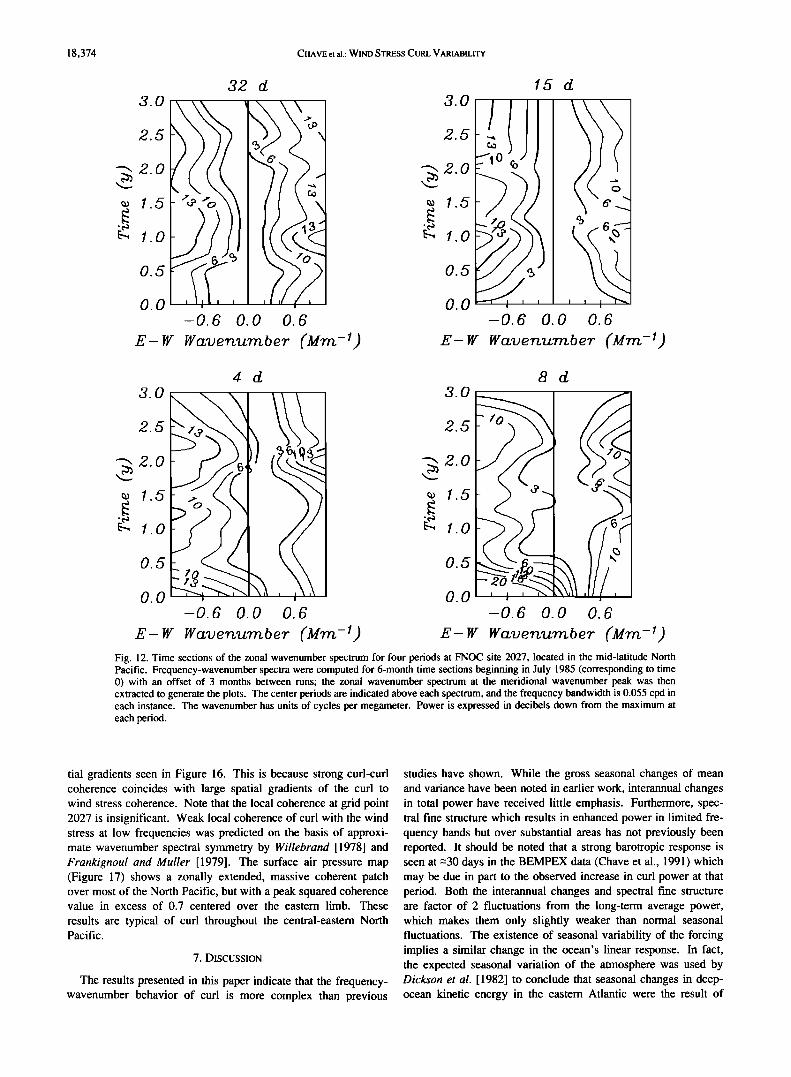
Fig. 12. Time sections of the zonal wavenumber spectrum for four periods at FNOC site 2027, located in the mid-latitude North Pacific. Frequency-wavenumber spectra were computed for 6-month time sections beginning in July 1985 (corresponding to time 0) with an offset of 3 months between runs; the zonal wavenumber spectrum at the meridional wavenumber peak was then extracted to generate the plots. The center periods are indicated above each spectrum, and the frequency bandwidth is 0.055 cpd in each instance. The wavenumber has units of cycles per megameter. Power is expressed in decibels down from the maximum at each period.

tial gradients seen in Figure 16. This is because strong curl-curl coherence coincides with large spatial gradients of the curl to wind stress coherence. Note that the local coherence at grid point 2027 is insignificant. Weak local coherence of curl with the wind stress at low frequencies was predicted on the basis of approximate wavenumber spectral symmetry by Willebrand [1978] and Frankignoul and Muller [1979]. The surface air pressure map (Figure 17) shows a zonally extended, massive coherent patch over most of the North Pacific, but with a peak squared coherence value in excess of 0.7 centered over the eastern limb. These

results are typical of curl throughout the central-eastern North Pacific.

7. DISCUSSION

The results presented in this paper indicate that the frequency- wavenumber behavior of curl is more complex than previous

studies have shown. While the gross seasonal changes of mean and variance have been noted in earlier work, interannual changes in total power have received little emphasis. Furthermore, spectral fine structure which results in enhanced power in limited frequency bands but over substantial areas has not previously been reported. It should be noted that a strong barotropic response is seen at --30 days in the BEMPEX data (Chave et al., 1991) which may be due in part to the observed increase in curl power at that period. Both the interannual changes and spectral fine structure are factor of 2 fluctuations from the long-term average power, which makes them only slightly weaker than normal seasonal fluctuations. The existence of seasonal variability of the forcing implies a similar change in the ocean's linear response. In fact, the expected seasonal variation of the atmosphere was used by Dickson et al. [1982] to conclude that seasonal changes in deep- ocean kinetic energy in the eastern Atlantic were the result of


32 d 3.0

0.•

0.0 -0.6 0.0 0.6

E-W Waver•u,e'r•bew (Mra -•)

3.0

2.5

'•, 2.0

1.5

•1.0

0.5

0.0

E-W

15d

-0.6 0.0 0.6'

4d 8d

3.0 xd ' 3.0 2.5 25

'•, 2.0 '•, 2 0 • o

E.o

O.5 O5

0.0 O0 -0.6 0.0 0.6' -0.6 0.0 0.6'

Fig. 13. Time sections of the zonal wavenumber spectrum at FNOC site 1830, located in the mid-latitude North Pacific. Frequency-wavenumber spectra were computed for 6 month time series beginning in July 1985 (corresponding to time 0) with an offset of 3 months between runs; ttie zonal wavenumber spectrum at the meridional wavenumber peak was then extracted to generate the plots. The inclusive time periods are indicated above each spectrum, and the frequency bandwidth is 0.055 cpd in each instance. The wavenumber has units of cycles per megameter. Power is expressed in decibels down from the maximum at each period. Note the similarities and differences with Figure 12.

direct atmospheric forcing, Deep-ocean seasonal kinetic energy fluctuations have also been noted by Niiler and Koblinsky [1985] for th e North Pacific, while Koblinsky et al. [1989] cite exaniples of interannual changes in oceanic energy levels that are correlated with the strength of curl. Thus, it appears that changes in the forcing by a factor of 2 will produce significant changes in the ocean's response. However, the BEMPEX data contain little evidence for seasonal changes in barotropic kinetic energy despite their location (41øN, 163øW) near the peak in curl variance, suggesting that other factors than curl power, such as fluctuating propagation direction, also play an important role in determining the ocean's response.

Perhaps the most important result of this work is the realization that wavenumber variability for curl may be substantial. This has implications for comparisons of models with oceanic data. For example, the peak wavenumbers for the 3-year averaged spectra

shown in Eigures 6-11 are not very different from the frequency- dependent mean wavenumbers inferred by Willebrand [1978]. It appears that the peak widths for the MLM spectra are larger, although comparisons are difficult because the standard error Of the mean wavenumber computed by Willebrand is not i'eally equivalent to spectral bandwidth. However, if the yearly average spectra in Figures 6-11 are compared with Willebrand's results, then differences arise as asymmetry becomes apparent for some data sections: This is even more obvious in the 6-month spectral time sections of Figures 12-13. Note also that differences between zonal and meridional variability, and especially the bandwidth as denoted by the main lobe width, are not readily detectable because of wavenumber variability. These observations SUggest that it is variability that determines many of the gross characteristics of curl, that the length of the analysis interval will affect the estimation of these characteristics, and that care is


, ,. _ 50 ø

• 22 ..

20

.g

½ 24 'ca

_

,

_

, I I 170ø1 ,' ... I \ 140 ø

40 35 30 25 20 40 35 30 25 20 Zonal Cr•d Point Zonal Cr•d Point

?/ss-?/s?

40 35 30 25 20 40 35 30 25 20

Zonal Grid Point Zonal Grid ?oi•t

Fig. 14. Maps of the squared coherence between curl at FNOC grid point 2027 and curl over the North Pacific Ocean at a period of 25 days for the 3-year interval 1985-i988 and individual years as noted above each plot. The coherence was computed using the multiple window method and possesses a bandwidth of 0.044 cpd for all four estimates. Because the degrees of freedom are different for the 3- and 1-year spectra, the zero coherence levels at 95% significance are 0.15 and 0.18, respectively. Values smaller than this were not included in the contouring process, and the remaining contours are at intervals of 0.1 beginning at 0.2. The coherence is 1 at 2027. Note the variability of both the main lobe shape (centered on grid point 2027) and the strength of the intercorrelation peaks.

required when inferring curl properties for inclusion in models. In particular, for a given time interval, differences between wavenumber spectra are observed over distances of --1200 km, as seen in Figures 12 and 13, suggesting that average curl models for an ocean basin are not entirely applicable.

As an ex.ample, it is interesting to contemplate the possibility that a winter of very strong curl amplitude could result in only a weak oceanic response if the zonal wavenumber spectrum were inordinately eastward, assuming that a resonant response is typi-

trate this. it should be remembered that the summer to winter

range in power is typically a factor of 2-4, so that curl power fluctuations inferred from directional changes in these examples are comparable to the seasonal range. Neither of these postulated short term changes in the ocean's response to atmospheric forcing would necessarily be predicted if longer-term average wavenumber spectra were used to force a model. This has obvious implicfi- tions for specific data to model comparisons. These results suggest that more attention should be paid to the characteristics of

cally stronger than an evanescent one. The fall-winter of curl during the time oceanic measurements are being taken rather 1987-1988 at site 1830 for 15 days period in Figure 13 (see 2.2-2.7 years in the figure) is a good candidate time period for such behavior. Of course, the reverse is also possible, and westward curl fluctuations might result in substantial increases in Rossby wave excitation when no corresponding power change occurs. The fall-winter of 1986-1987 at 1830 for a 15 or 32 day period in Figure 13 (see 1.3-1.7 years in the figure) might illus-

than to long-term curl statistics. However, this might be miti- gated somewhat by the weak tendency for long-term average wavenumber spectra to display wider peak widths than shorter ones. The wider peak width will result in an increase in westward power that will at least partially compensate for the lack of speci- ficity.

A number of differences between the curl wavenumber obser-

CHAVE eta!.: WIND STRESS CURL VARIABILITY 18,377

• 24

r• 22

.,., 20

18

½16

• 22

' .• 20 - ao

40 35 30 25 20 40 35 30 25 20 Zona. l Grid Point Zonal Grid Point

• 24

• 22

40 35 30 25 20

Zonal Grid Point

• 24

.• 20

,'•12, !00 o

?- ?

ß

! ?Oø I ,' •.. I

/50 a

\ 140 •'

40 35 30 25 20

Zonal Grid Point

Fig. 15. Maps of the squared coherence between curl at FNOC grid point 2027 and curl over the North Pacific Ocean at a period of 25 days for the four seasons beginning in July 1986, as noted above each plot. The coherence was computed using the multiple window method and possesses a bandwidth of 0.044 cpd, identical to that for Figure 14. The zero coherence level at 95% significance is 0.39; values smaller than this were not included in the con.touring process. The remaining contours are •at intervals of 0,1 beginning at 0.5. The coherence is 1 at 2027. Note the variability of both the main lobe shape (centered on grid point 2027) and the strength of the intercorrelation peaks.

vations of this paper and both prior observations and models have been noted. First, the average spectral shape, and especially the high-wavenumber slope, are not comparable to those computed by Gallegos-Garcia et al. [1981] using a conventional (Fourier- based) wavenumber estimator. Their composite wavenumber estimate from 11 years of monthly wind observations was nearly symmetric, did not display wavenumber independence at large scales, and falls off approximately like k -'/-'. By contra•t, MacVeigh et al. [1987], also using a conventional wavenumber estimator applied at unspecified frequencies, got a white result for scales larger than --1200 km (0.83 Mm-1 in the units of Figures 6-14) and• a =k -4 slope •at shorter wavelengths. No significant variation with season was reported. This is in qualitative agreement with the results of this paper. However, the flat part of the MacVeigh et al. spectrum appears to have a wider but variable width, possibly because their conventional wavenumber estimator could not adequately resolve large-scale features. No attempt has been made to compute an average spectral slope in the present study on account of marked directional variability. However, both the zonal and meridional wavenumber spectra clearly are quite red for wavenumbers larger than 0.2-10.6 Mm -1 (wavelengths of 1700-5000 km).

Note also that neither these observations nor those of

MacVeigh et al. [1987] agree with the curl wavenumber parame- terization derived largely from tropospheric measurements by Frankignoul and Muller [1979] and adopted for the Muller and Frankignoul [1981] atmospheric forcing simulation. North of 35 ø, their model is symmetric and has a spectral slope of k 4 from zero wavenumber to that characteristic of baroclinic instability in the atmosphere (equivalent wavelength of 5000 km), falls off with inverse wavenumber to a high-wavenumber cutoff corresponding to a scale smaller than the oceanic motions of interest, and zero

beyond. This contains more short-scale (<5000 km) power than real curl based on actual wavenumber estimates. As a conse-

quence, more short Rossby waves will be present in their model than in the real ocean, resulting in an increased wavenumber bandwidth and reduced coherence between oceanic and atmo-

spheric variables. However, assuming a high-frequency wavenumber cutoff of 2•r/500 km appropriate for the FNOC product, the Frankignoul and Muller spectral model yields a white noise level of 1.04x10 -14 dyn 2 cm -6 d which is in good agreement with Figures 4-5. This suggests that while there may be a discrepancy in the wavenumber distribution of power, its integral is in agreement.


24

22

ZonzL C?t Point

curl

22 ß

(

.½.

40 35 30 25 20

Zonal Grid Point

curl ? with ps

Fig. 16. Maps of the squared coherence between curl at FNOC grid point 2027 and the zonal (top) and meridional (bottom) wind stress over the North Pacific ocean at a period of 25 days for July 1986 to June 1987 inclusive. The coherence was computed using the multiple window method'with a bandwidth of 0.022 cpd, yielding = 14 degrees of freedom at each frequency for a zero coherence level of 0.39 at 95% confidence. Val- ues smaller than this were not included in the contouring process, and the remaining contours are at intervals of 0.1 beginning at 0.5. The phase of the coherence is consistent with the relationship expected from (2); see text for discussion.

30 25 20

Fig. 17. Map of the squared coherence between curl at FNOC grid point 2027 and the surface air pressure over the North Pacific Ocean at a period of 25 days for July 1986 to June 1987 inclusive. The coherence was computed using the multiple window method with a bandwidth of 0.022 cpd, yielding =14 degrees of freedom at each frequency for a zero coherence level of 0.39 at 95% confidence. Values smaller than this were not

included in the contouring process.

scale in the zonal (=1000 km) than in the meridional (=300 km) directions. Samelson used a simpler double exponential with comparable e-folding scales which was based on spatdally averaged curl coherence maps. While Samelson's maps do not show any secondary lobes, it is likely that the spatial averaging would remove them. Note that the different zonal and meridional scales

are not supported by this study. Both of these functions have a single peak at the origin, and cannot reproduce the secondary lobes seen in Figures 14-15. However, the presence of secondary peaks will have important ramifications for the oceanic response, especially if they are located to the east of the oceanic measure- ment and hence can resonantly excite long Rossby waves, assuming the frequency-wavenumber characteristics are appropriate. This suggests that the Brink and Samelson models probably underrepresent the oceanic response to atmospheric forcing. Sim- ilarly, the Muller and Frankignoul [1981 ] model does not include the effect of curl intercorrelation. The complex spatial structure of curl and its temporal fluctuations are just additional manifesta- tions of a spatdally ,inhomogeneous and variable wavenumber spectrum, and can be accounted for either in the spatial or wavenumber domains. However, simple parameterizations chosen for analytic simplicity are probably inadequate to reproduce the real properties of curl.

Finally, the observation that the curl intercorrelation possesses both a relatively tight main lobe and a number of nonlocal peaks has further implications for the oceanic response. Since the spatial variation of the squared coherence of curl at a given frequency as in Figures 14-15 is comparable to the square of its autocorrelation function (of course, values smaller than the zero significance level which are not shown in the figures must be included), comparisons with the analytic curl models used by Brink [1989] and Samelson [1989, 1990] may be made directly. Brink modeled the curl autocorrelation as a double Gaussian with a larger e-folding

Acknowledgments. The authors are grateful to David J. Thomson of Bell Laboratories for suggesting the Bartlett M test and providing general statistical advice. This work was supported at SIO by National Science Foundation grants OCE-8420578, OCE-8800783, and OCE-8922948.

REFERENCES

Bartlett, M.S., Properties of sufficiency and statistical tests, Proc. R. $oc. London, $er. A, 160, 268-282, 1937.

Brink, K.H., Evidence for wind-driven current fluctuations in the western North Atlantic, J. Geophys. Res., 94, 2029-2044, 1989.

Capon, J., High-resolution frequency-wavenumber spectrum analysis, Proc. IEEE, 57, 1408-1418, 1969.


Capon, J., and N.R. Goodman, Probability distribution for estimators of the frequency-wavenumber distribution, Proc. IEEE, 58, 1785-1786, 1970.

Chave, A.D., D.J. Thomson, and M.E. Ander, On the robust estimation of power spectra, coherences, and transfer functions, J. Geophys. Res., 92, 633-648, 1987.

Davis, R.E., and L. Regier, Methods for estimating directional wave spectra from multi-element arrays, J. Mar. Res., 35, 453-477, 1977.

De Young, B., and C.L. Tang, An analysis of Fleet Numerical Oceanographic Center winds on the Grand Banks, Atmos. Ocean, 27, 414-427, 1989.

Dickson, R.R., W.J. Gould, P.A. Gurbutt, and P.D. Killworth, A seasonal signal in ocean currents to abyssal depths, Nature, 295, 193-198, 1982.

Ehret, L.L., and J.J. O'Brien, Scales of North Atlantic wind stress curl determined from the Comprehensive Ocean-Atmosphere Data Set, J. Geophys. Res., 94, 831-841, 1989.

Frankignoul, C., and P. Muller, Quasi-geostrophic response of an infinite [3-plane ocean to stochastic forcing by the atmosphere, J. Phys. Oceanogr., 9, 104-127, 1979.

Friehe, C.A., and S.E. Pazan, Performance of an air-sea interaction buoy, J. Appl. Meteorol., 17, 1488-1497, 1978.

Gallegos-Garcia, A., W.J. Emery, R.O. Reid, and L. Magaard, Frequency- wavenumber spectra of sea surface temperature and wind-stress curl in the eastern North Pacific, J. Phys. Oceanogr., 11, 1059-1077, 1981.

Halliwell, G.R., Jr., and P. Cornilion, Large-scale SST variability in the western North Atlantic subtropical convergence zone during FASINEX. Part I: Description of SST and wind stress fields, J. Phys. Oceanogr., 20, 209-222, 1990.

Harrison, D.E., On climatological monthly mean wind stress and wind stress curl fields over the world ocean, J. Clim., 2, 57-70, 1989.

Koblinsky, C.J., P.P. Niiler, and W.J. Schmitz, Jr., Observations of wind- forced deep ocean currents in the North Pacific, J. Geophys. Res., 94, 10773-10790, 1989.

Kousky, V.E., and A. Leetmaa, The 1986-87 Pacific warm episode: Evolution of oceanic and atmospheric fields, J. Clim., 2,254-267, 1989.

Large, W.G., and S. Pond, Open ocean momentum flux measurements in moderate to strong winds, J. Phys. Oceanogr., 11,324-336, 1981.

Lewis, J.M., and T.H. Grayson, The adjustment of surface wind and pressure by Sasaki's variational matching technique, J. Appl. Meteorol., 11,586-597, 1972.

Luther, D.S., A.D. Chave, and J.H. Filloux, BEMPEX: A study of barotropic ocean currents and lithospheric electrical conductivity, Eos, Trans. AGU, 68, 618-619, 628-629, 1987.

Luther, D.S., A.D. Chave, J.H. Filloux, and P.F. Spain, Evidence for local and nonlocal barotropic responses to atmospheric forcing during BEMPEX, Geophys. Res. Lett., 17, 949-952, 1990.

MacVeigh, J.P., B. Barnier, and C. Le Provost, Spectral and empirical orthogonal function analysis of four years of European Center for

Medium Range Weather Forecast wind stress curl over the North Atlantic Ocean, J. Geophys. Res., 92, 13141-13152, 1987.

Muller, P., and C. Frankignoul, Direct atmospheric forcing of geostrophic eddies, J. Phys. Ocean., 11,287-308, 1981.

Niiler, P.P., and C.J. Koblinsky, A local time-dependent Sverdrup balance in the eastern North Pacific, Science, 229, 754-756, 1985.

Pazan, S.E., T.P. Barnett, A.M. Tubbs, and D. Halpern, Comparison of observed and model wind velocities, J. Appl. Meteorol., 21, 314-320, 1982.

Philander, S.G.H., Forced oceanic waves, Rev. Geophys., 16, 15-46, 1978. Rienecker, M.M., and L.L. Ehret, Wind stress curl variability over the

North Pacific from the Comprehensive Ocean-Atmosphere Data Set, J. Geophys. Res., 93, 5069-5077, 1988.

Samelson, R.M., Stochastically forced current fluctuations in vertical shear and over topography, J. Geophys. Res., 94, 8207-8215, 1989.

Samelson, R.M., Evidence for wind-driven current fluctuations in the eastern North Atlantic, J. Geophys. Res., 95, 11359-11368, 1990.

Terada, K., and M. Hanzawa, Climate of the North Pacific Ocean, in Worm Survey of Climatology, vol. 15, edited by H. Van Loon, pp. 431-504, Elsevier, New York, 1984.

Thomson, D.J., Spectrum estimation and harmonic analysis, Proc. IEEE, 70, 1055-1096, 1982.

Trenberth, K.E., J.G. Olson, and W.G. Large, A global ocean wind stress climatology based on ECMWF analyses, NCAR Tech. Note TN- 338+STR, 93 pp., Nat. Cent. for Atmos. Res., Boulder, Colo., 1989.

Wilkerson, J.C., and M.D. Earle, A study of differences between environmental reports by ships in the voluntary observing program and measurements from NOAA buoys, J. Geophys. Res., 95, 3373-3385, 1990.

Willebrand, J., Temporal and spatial scales of the wind field over the North Pacific and North Atlantic, J. Phys. Oceanogr., 8, 1080-1094, 1978.

Willebrand, J., S.G.H. Philander, and R.C. Pacanowski, The oceanic response to large-scale atmospheric disturbances, J. Phys. Oceanogr., 10, 411-429, 1980.

Willson, M.A.G., A wavenumber-frequency analysis of large-scale tropospheric motions in the extratropical northern hemisphere, J. Atmos. Sci., 32,478-488, 1975.

A.D. Chave, Woods Hole Oceanographic Institution, Woods Hole, MA 02543.

J.H. Filloux and D.S. Luther, Scripps Institution of Oceanography, Mail Code 0230, La Jolla, CA 92093.

(Received May 13, 1991; revised August 15, 1991;

accepted August 15, 1991.)

variability of the wind stress curl over the north pacific

Documents