Vanishing Point Detection

A Tai, J Kittler, M Petrou and T WindeattDept. of Electronic and Electrical Engineering,

University of Surrey,

Guildford, Surrey GU2 5XH, United Kingdom

Abstract

Commencing with a review of methods for vanishing point (VP) detec-tion, a new approach is suggested. The proposed approach estimatesthe location of candidate vanishing points and provides probabilitymeasures which reflect the likelihood of those points being the VPs.This new approach allows VPs to be identified in less structured envi-ronments compared with its conventional counterparts.

1 IntroductionGeometrical cues and constraints provide valuable information as to how certainimage features should be interpreted. For instance, in many man made scenesthere exist a number of straight lines which are mutually parallel in 3D. Underperspective projection these lines will meet at a common point known as thevanishing point (VP). Once this point is identified, one can infer 3D structuresfrom 2D features and this constrains the search for other structures. Also,under known camera geometry the orientation of the lines that are groupedtogether can be determined from the corresponding VP. Furthermore, two ormore vanishing points arising from lines which lie on a certain 3D plane givea vanishing line. This property provides an additional constraint which isparticularly relevant when analysing, for instance, aerial imagery where onecan often assume that structures of interest lie in a common plane - the groundplane.

The relationships amongst camera parameters, structures in 3D scenes andVPs had been established by Haralick [1]. The applications of VP analysisranges from extracting 3D structures to the calibration of camera parameters.

An obvious approach to locating VPs is to exploit directly the property thatall lines with the same orientation in 3D converge to a VP under perspectivetransformation. Thus the task of VP detection can be treated as locating peaksin a two dimensional array where the intersections of all line pairs in an imageplane accumulate. However, the line pairs can intersect anywhere from pointswithin an image to infinity and this poses problem on implementation.

In order to avoid analysing an open space Barnard proposed the projectionof image lines onto a Gaussian sphere [2] [3] [4] which neatly represents any 3Dorientations. The plane which contains the lens centre and the line segment inthe image intersects with the Gaussian sphere centred at the origin to form agreat circle. That is a line segment on the image plane is mapped to a great

BMVC 1992 doi:10.5244/C.6.12

110

circle. Hence, VPs can be detected as elements on the surface of the Gaussiansphere which have relatively high votings. Obviously, the Gaussian surface hasto be partitioned in order to accumulate votes. One popular parameterisationis in terms of the azimuth and elevation angles of the unit vector in the sphere.Note that a uniform partitioning in the Hough space maps to non-uniform areain the image plane. For example, the elementary areas at the poles are smallcompared with those at the equator. This implies that some lines may intersectwithin a larger area and still be grouped together to hypothesise a VP whereasothers may not. A crude way of ensuring accuracy is to partition the Houghplane into finer bins. This improvement in accuracy is paid for by an increasein memory requirement and computational load.

Magee et al [3] compute the vectors pointing towards the intersection of linesegments in the image plane using a series of cross-product operations. Insteadof incrementing a discrete parameterisation, the actual values of the azimuthand elevation angles are maintained for comparison using an arc distance asa metric. This circumvents the problem of the non-uniform elemental surfacearea of the Gaussian sphere. Although this allows one to locate VPs to a higheraccuracy, the computation of the vectors pointing at the intersection points hastransformed the O(n) order problem to an O(n2) one.

Quan and Mohr [4] propose an efficient way both in terms of the amount ofoperations and memory requirement for computing VPs. They employ a pyra-midal data structure instead of a straight forward two dimensional array. Thisalgorithm is similar to a Fast Hough Transform method. It consists of subdi-viding recursively a patch on the sphere into 4 sub-patches from a coarse to fineresolution. By doing so, a coarse to fine algorithm can be used to improve theefficiency of the Hough Transform (HT). However, detailed experimental stud-ies of hierarchical approaches to the vote accumulation in the HT suggest thatthe steps that need to be taken to ensure the detection of all level features mayrender the technique computationally inferior to standard HT implementation.

The methods outlined above do not handle the issue of noise directly, insteadthe locations of the vanishing points are assumed to be the mid-point of thebin. Thus, the error of the estimated locations of VPs is a function of bindimensions. Collins and Weiss [5] treat the task of VP detection as a statisticalestimation problem. They note that a vector pointing towards the VP lies inthe projection plane of the line, and is thus perpendicular to the projectionplane normal. In other words, the projection plane normals of 3D parallel lineslie in a plane through the origin, perpendicular to the orientation of the 3Dlines in a noiseless environment. In reality, these normals cluster around a greatcircle forming an equatorial distribution and this distribution is then modelledusing Bingham's distribution [6]. It turns out that this approach gives the sameresult as fitting the least squares perpendicular error planes corresponding tothe line pairs.

VPs are also widely used for camera calibrations and recovery of rotationalcomponent of motion. Camera calibration involves the determination of camerarotation and translation matrix, focal length etc. These rely on the relationshipsbetween the VP coordinates and the camera parameters both intrinsic andextrinsic. The usefulness of VPs in motion analysis stems from the fact thatthey represent 3D orientations and are therefore invariant to 3D translationsbetween the camera and the scene.

Liou and Jain [7] devised a scheme for road tracking in image sequences.

111

Assuming that the locations of VP remains unchanged in contiguous frames,they then fit a template around this VP. The dimensions of this templateare determined by a constant and a tilt angle. Since the true VP must fallinside this area, one can locate the road boundaries by considering a pair ofconvergent lines which maximises an ad hoc measure based upon the lengths oflines, directions of edge points supporting the lines etc.

Shigag et al [8] compute camera rotation by first classifying lines on theimage into horizontal and non-horizontal groups and then estimating the cam-era rotation as the difference of the angle between the optical axis and the 3Dorientation of a certain horizontal line. This method takes advantage of theproperty of vanishing line (vanishing line is the locus of VPs for all lines lieon the same plane). To identify whether a line is horizontal or not, two con-straints are applied: (1) horizontal lines should not intersect the vanishing line,(2) locus of VPs of horizontal lines are different from that of non-horizontalones.

Wang and Tsai [9] proposed an approach to camera calibration based uponthe use of vanishing lines. This technique requires only a single view of a cube.The three principle vanishing points (i.e. VPs that correspond to the orthogonaldirections of the world coordinates) are detected and the orthocentre of thetriangle thus formed gives the image plane centre. This provides a neat wayfor calibration. The camera orientation parameters are determined from theslopes of the lines forming the triangle. In addition to these they also establishthe relationship between the area of the vanishing triangle for calibration offocal length.

In summary, all existing methods for extraction of VPs perform some formof accumulation of line pair junctions. With the Gaussian sphere parameter-isation being most popular, while this is a valued approach, there are severalshortcomings associated with it.

As bins in the Hough plane map to non-uniform area on the image plane,some intersection points are grouped together under a more stringent conditionthan others depending on the locations of the VPs. Problem also arises whenvotes fall into neighbouring bins which might cause a significant peak to dimin-ish in strength. However, most important of all is that accuracies of detectedlines are ignored. As far as VPs are concerned the positional and orientationalerrors cause incorrect intersection points to be formed which reduce the strengthof the 'true' peaks and give rise to spurious intersection points which might inturn group with other points to produce 'false' vanishing points. Additionally,this would also disperse intersection points (as the bin size has an impact onHough Transform) which inherently belong to the same VP. The above pointsshow the sensitivity of this approach to noise. Furthermore, due to the na-ture of the algorithm any convergent group which consists of a relatively smallnumber of 3D parallel lines would be left undetected.

Most papers on the topic, analyse images of scenes such as offices and cor-ridors which are highly structured and have strong perspective. Consequently,there are less potential VPs and the strength of true VPs are significantly higherthan the background and are therefore distinguishable from random intersec-tions.

More recently, Brillault-O'Mahony [10] took into consideration the uncer-tainty in the detection of line segments and designed an isotropic accumulatorspace where the probability of erroneous VP detection is uniformly distributed

112

(a) (b)

(c)

Figure 1: (a) Original image (b) Hough Transform output (c)Hough Plane accumulation of the azimuth and elevation angles.

throughout all the cells. In any case, the approach is still based on the accu-mulator array idea and thus is inappropriate for images with sparse parallellines.

However, there are many domains of applications where the scene containsonly a few lines which are parallel in 3D and on such imagery the existingtechniques gave results as illustrated in fig.l. Fig.l(c) shows that there is nodominant peak for the set of lines shown in fig.l(b).

This paper proposes a method which takes a different perspective to detect-ing vanishing points. Instead of accumulating intersection points, we computethe probability of a group of lines passing the same point. This approach pro-vides a probability measure for discriminating between competing hypothesesirrespective of the size of the vanishing group. In addition, its performance alsodegrades gracefully in noisy environments. The paper is organised as follows,Section 2 of this paper introduces a novel vanishing point detection method.In Section 3, a probabilistic line representation which is a prerequisite of themethod developed. In section 4 we present the experimental results and finally,section 5 offers some conclusions and discussion.

2 Vanishing Point DetectionLet us consider an image with line segments represented by p — 0 parameter-isation. Due to the geometrical constraints dictated by the image formationprocess, all perspectively projected line segments having the same orientation

113

in three space converge to a single point - the vanishing point - in the imageunder a noise free condition. However, both the imaging and low level edge andstraight line extraction processes are inherently noisy resulting in uncertaintiesin the p and 6 parameters of the detected lines. Errors in p and 9 will result ina considerable scatter of the intersection points of the pairs of lines segmentswhich makes it difficult to identify true vanishing points. As pointed out ear-lier, this problem is particularly pertinent when the scene structure containsonly a small number of parallel lines.

In this paper the search for vanishing points makes an explicit use of distri-bution models of the parameters of the detected lines. With such a probabilisticdescription for each line we can pose the question of how likely a given pointis the common intersection point of a group of lines. In this manner for anyselected group of lines we can determine the probability distribution p(x, y) fortheir mutual intersection point (x,y). A vanishing point is then identified asthe point of maximum of this probability distribution function which exceedssome pre-specified threshold.

Let us start by considering a single line with parameters (/>;, 9i) and let thedistribution of errors 8p,89 in pi and B{ be pi(6p,69) respectively. Now theprobability of the line passing through a point (x, y) in the image will be givenby compounding all the combinations of errors 8p and 69 such that the trueline with parameters

p = pi+8p (1)

9 = 9i+69 (2)

satisfies the constraint equation

p = x cos 9 + y sin 9 (3)

the compound probability Pi(x, y) is thus given by

Pi(x,y) = | [Pi(6p,69)ds (4)zi J s

where the integration is performed in the parameter space along the sinusoidalline defined by (3) and z; is the normalising constant to ensure that Pi(x,y)is a probability density function. In terms of parameter errors the compoundprobability can be expressed as

Pi(x,y) = L J* Pi{8p, 86)^1+ {^yd9 (5)

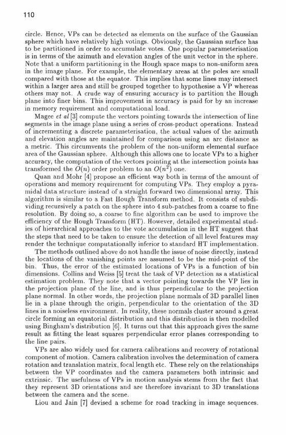
The compounding process is illustrated in fig.2.Now let X = {ei\i = 1, 2, ...k} be a group of lines selected from the best of

lines output by an image description process, with the measured parameters foreach line denoted by vector w,- = [pi,9i]T and the associated error distributionby pi(8p,89). By analogy the probability that the lines jointly pass througha point (x,y) in the image plane (which extends beyond the physical imagingarea of the sensor) is given by

P(x,y) = - / Pi(6p,89)Jl + (-£)2d9 (6)± ± -r . I \l sill ^ '

114

Figure 2: Rectangular probability density function.

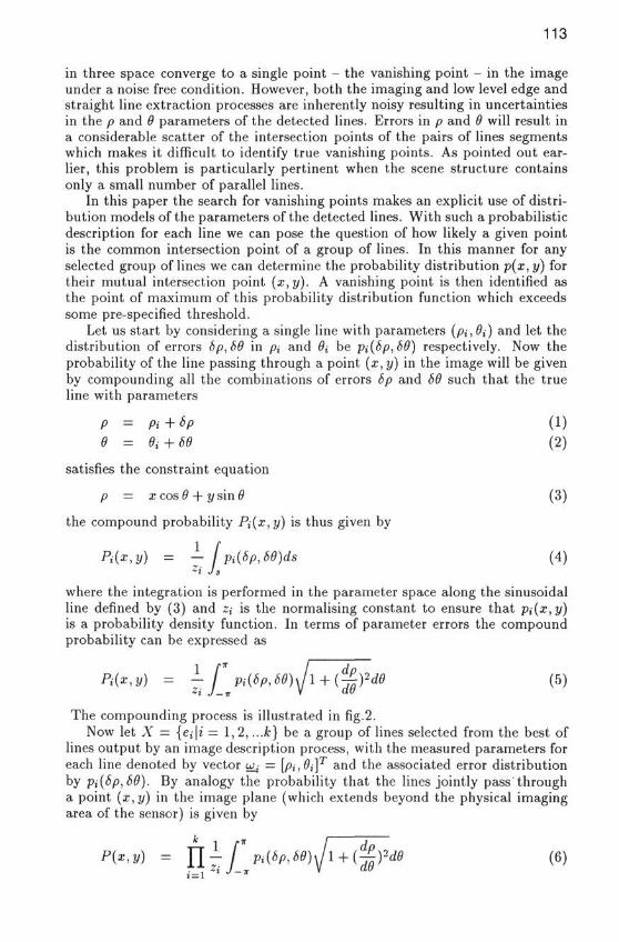
Figure 3: Evidential Support.

From the knowledge of pt(6p, 69) the probability of P(x, y) can easily be eval-uated. Its mode (xv,yv) then defines a vanishing point provided P(xv,yv) isabove the threshold.

In order to develop a practical procedure based on the above idea we firstneed to select a suitable groups of lines. Regarding these lines, the method isintended for finding vanishing points of small sets of 3D parallel lines, hence thecardinality of the group should be quite small. Moreover, the computationalcomplexity of the problem could potentially grow combinatorially with thenumber of lines in the group. In the present approach the initial analysis isperformed for line triplets. Any larger group of lines is formed after this firstanalysis stage by considering the proximity of detected vanishing points andthe overlap of the two participating line sets.

To prune the set of all possible triplets each candidate group of lines mustsatisfy a number of criteria. These include

1. angular constraints (similarity of 0t- values)

2. distance constraint (the perpendicular distance of line pair intersectionpoint from the third line)

3. junction quality constraint [ll](the lines should intersect at a point whichis remote from all participating line endpoints as illustrated in fig.3.)

4. imaging geometry constraints (if known)

115

3 Probabilistic Line Representation

In the light of the discussion in the previous section we require an appropriateline representation which can associate uncertainties with its parameters. It isimportant that this representation is easy to convert to and from the standardHough Transform(HT) p — 9 space representation, since we use this method forthe extraction of straight lines.

The parametric representations that we adopted for a perfect line are eitherv\ = [p, 1,9, L] or v2 = [xm,ym,9,L] , where p is the distance between thefoot of the normal and the origin, / is the distance from the foot of the normalto the line midpoint; 0 and L are the line orientation and length respectively.Xm,ym are the coordinates of the line midpoint.

Deriche and Faugeras [12] also address the issue of finding an appropriateline representation. Their conclusion is that vector v-x is a more favourablechoice than vector v\ simply because representation v\ leads to a covariancematrix that strongly depends upon the position of the associated line segment inthe image through the effect of p and /. Hence, from this standpoint v\ does notallow different Kalman filters to be applied on each parameter. However, as faras our application is concerned it does not matter what the interactions betweenvarious parameters are. We only need the necessary statistical parameters tobuild the error models which we can utilise for the development of a formalapproach to VP detection.

A simple analysis involving Taylor series expansion leads to the followingapproximate relationship between the errors in line orientation, line midpointand the distance from the origin to the foot of the normal:

6p = — (xm s\n9 — ym cos9)86 + 6xcos9 + 6ysin9 (7)

Note that in deriving the above equation, we assume that any terms involvingthe cross product of positional and orientational errors can be neglected. Forlines four pixels long or more the quadratic terms become negligible. Equation(7) then gives a linear relationship between the errors in orientation 9 andline segment midpoint position and the errors in p. Thus if 69, 6x and 8y arenormally distributed, so will the errors p.

A Monte Carlo experiment was performed to check the validity of the ap-proximate model and its dependence on line length. From table 1 it is apparentthat provided the line length L >= 4 the linear model yields a distribution oferrors 8p with negligible skew and curtosis which can be taken to imply that itclosely approximates a Gaussian. Thus if 89, 8x and 8y are Gaussian, the jointdistribution of 8p, 86 and 81 will be Gaussian with covariance matrix

lag^ + az -lag (sin26)al - Ipag \- W <T»2 P°e2 (8)

sinzu)a~ — lpa$ pag p oe + cr /

Note that ax2 = ay

2 — a2. From (8) the distribution of interest p(6p,69) isnormal with zero mean and covariance matrix

(9)

116

Linexm = -36.6, ym = 136.6,6 = 150°

Firstorder

approx.

L = 1.0L = 4.0L = 10.0

mean (p)

0.061990.014410.00489

stdev (op)

8.773102.400761.33047

skew ((73)

-0.011720.006180.02300

curtosis (<74)

0.10832-0.07306-0.03726

Table 1: Statistical results of error in pCarlo experiment.

(Sp) obtained from Monte

where N is the number of points providing evidential support for the line. Notethat N may differ form L, the line length as some pixels inside the line seg-ment may be undetected. The covariance matrix in (9) applies if the HoughTransform (HT) line detection scheme has an optimisation facility to estimatethe most likely values of p and 6. When the standard HT is used with p and 6parameter quantisation, the probability distribution p(6p, 86) is no longer Gaus-sian. Instead its shape may vary from the rect to roof function depending onthe coarseness of the quantisation process. A study of the relative merits of thevarious detection schemes and the associated probabilistic line representationsis beyond the scope of this paper.

4 Experimental Results

The method was applied to aerial imagery of resolution 256X256. The rectan-gular line parameter probability distribution was used in the experiment.

The implementation involved the following steps:

1. Compute the intersection points of all possible pairs and discard thosethat fall outside the virtual image (this is an imaginary image of size512X512 centred at the origin).

2. Combine a line with a pair to create a triplet to see if it satisfies thepursuing constraints of section 2.

3. Set up a window around the line pair intersection point and computethe probability P{x,y) for all (x,y) in the window. Find the mode ofP(x,y) - (xv,yv).

4. Repeat steps (2) and 3 for all other triplets.

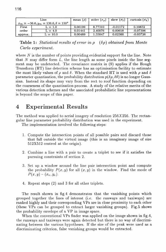
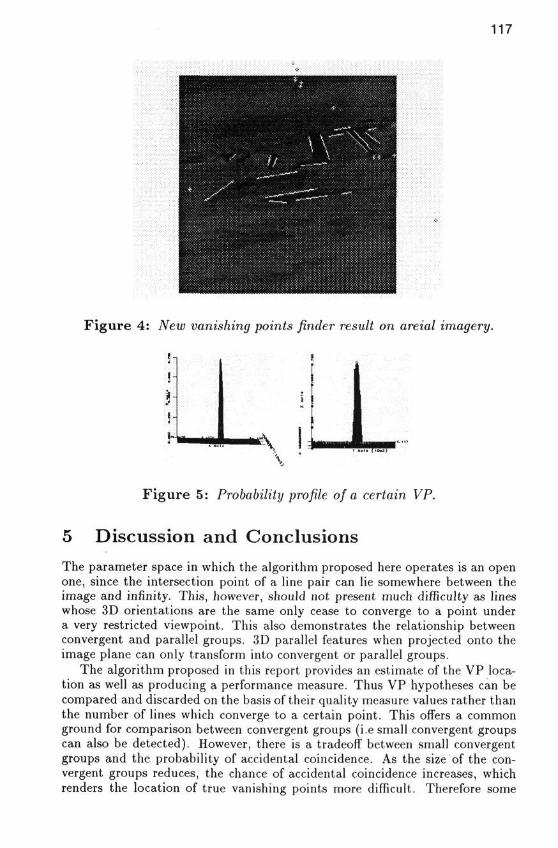
The result shown in fig.4 demonstrates that the vanishing points whichgrouped together the lines of interest (i.e. the runways and taxiways) areranked highly and their corresponding VPs are in close proximity to each other(these VPs can be grouped to extract larger vanishing groups). Fig.5 showsthe probability envelope of a VP in image space.

When the conventional VPs finder was applied on the image shown in fig.4,the runways and taxiways were again detected but there is no way of discrimi-nating between the various hypotheses. If the size of the peak were used as adiscriminating criterion, false vanishing groups would be extracted.

117

Figure 4: New vanishing points finder result on areial imagery.

£

Figure 5: Probability profile of a certain VP.

5 Discussion and Conclusions

The parameter space in which the algorithm proposed here operates is an openone, since the intersection point of a line pair can lie somewhere between theimage and infinity. This, however, should not present much difficulty as lineswhose 3D orientations are the same only cease to converge to a point undera very restricted viewpoint. This also demonstrates the relationship betweenconvergent and parallel groups. 3D parallel features when projected onto theimage plane can only transform into convergent or parallel groups.

The algorithm proposed in this report provides an estimate of the VP loca-tion as well as producing a performance measure. Thus VP hypotheses can becompared and discarded on the basis of their quality measure values rather thanthe number of lines which converge to a certain point. This offers a commonground for comparison between convergent groups (i.e small convergent groupscan also be detected). However, there is a tradeoff between small convergentgroups and the probability of accidental coincidence. As the size of the con-vergent groups reduces, the chance of accidental coincidence increases, whichrenders the location of true vanishing points more difficult. Therefore some

118

kind of geometrical cue is needed to recover true vanishing points. Vanishinglines are powerful cues to be exploited for the purpose. They are defined as thelocus of VPs formed by 3D parallel groups which lie on the same plane. Thisproperty means that the hypothesised points must lie on the vanishing line andthereby provide a constraint for discarding false VPs.

References[1] R.M. Haralick. Using perspective transformation in scene analysis. Com-

puter Graphics Image Processing, 13:191-221, 1980.

[2] S.T. Barnard. Methods for interpreting perspective images. In Proc. ImageUnderstanding Workshop, pages 193-203, Palo Alto, California, Sept 1982.

[3] M.J. Magee and J.K. Aggarwal. Determining vanishing points fromperspective images. Computer Vision, Graphics and Image Processing,26:256-267, 1984.

[4] L. Quan and R. Mohr. Determining perspective structures using hierachi-cal hough transform. Pattern Recognition Letters, 9(4):279-286, 1989.

[5] R.T. Collins and R.S. Weiss. Deriving line and surface orientation bystatistical methods. In Proc. Image Understanding Workshop, pages 433-438, 1990.

[6] R.T. Collins and R.S. Weiss. Vanishing point calculation as a statisti-cal inference on the unit sphere. Computer Vision, Graphics and ImageProcessing, pages 400-403, 1990.

[7] S. Liou and R. Jain. Road following using vanishing points. Proc. IEEEComputer Society Conference on Computer Vision and Pattern Recogni-tion, pages 41-46, 1986.

[8] L. Shigag, S. Tsuji, and M. Imai. Determining of camera rotation fromvanishing points of lines on horizontal planes. Computer Vision, Graphicsand Image Processing, pages 499-502, 1990.

[9] L. Wang and W. Tsai. Computing camera parameters using vanishing-line information from a rectangular parallelepiped. Machine Vision andApplications, (3):129-141, 1990.

[10] B. O'Mahony. A Probabilistic Approach to 3D Interpretation of MonocularImages. PhD thesis, City University, London, 1992.

[11] A. Etemadi, J-P. Schmidt, G. Matas, J. Illingworth, and J. Kittler. Low-level grouping of straight line segments. In Proc. British Machine VisionConference, pages 118-126, 1991.

[12] R. Deriche and O. Faugeras. Tracking line segments. ECCV, pages 259-268, 1990.

AcknowledgementsThe authors wish to acknowledge support by the Procurement Executive, Min-istry of Defence for this work.