valuing innovation-based investments with the … · 2/4/2017 · valuing innovation-based...

Valuing Innovation-Based Investments with the

Weighted Average Polynomial Option Pricing

Model.

Elena Rogova1, Andrey Yarygin

2

National Research University Higher School of Economics,

55-2 Sedova Ulitsa, Saint-Petersburg 192171, Russia

April, 23, 2012

Abstract.

This paper contains the analysis of pitfalls connected with innovation-based investments

valuation. Being long-term projects with high uncertainty, innovation-based investments

suffer from different types of mistakes if traditional discounted cash flow methodology is

used for their valuation. The real options approach is being used for a long time, but this paper

proposes an original approach based upon the consideration of the wide variety of project

implementation scenarios. The weighted average polynomial option pricing model presented

here may help investors to increase the quality of decisions concerning their participation in

innovation-based opportunities.

JEL classification: D81, D92, G32.

Keywords: Real Options, Investment Valuation, Black-Scholes Option Pricing Model

(BSOPM), Cox-Ross-Rubinstein Binomial option pricing model (BOPM), Weighted Average

Polynomial Option Pricing Model (WAPOPM).

1 Dr. of Economics, Professor. E-mail: [email protected]

2 Post-graduate student. E-mail: [email protected]

1. Introduction.

The strongest companies in different sectors of economy demonstrate leading market position,

high return on assets and equity, rapid capitalization growth. Their success could be explained

mostly by creation, transfer, and commercialization of unique technologies. Undoubtedly, it is

a very attractive course of development for any company and for any economy (look, for

example, Tsujimura (2010) and Ettlie (1998) papers for more details). However high-

technology projects differ from traditional investments by the next features:

Extended uncertainty – very often cash flow has irregular nature, i.e. no reliable

hypothesis about the probability distribution of key parameters could be formulated;

Problems in strategic effect valuation – this effect may have more qualitative than

quantitative character and hardly can be valuated with reliable figures.

Discounting Cash Flow Method (DCF) with Net Present Value (NPV) as a main criterion is

the most widespread analytical tool for the Investments Valuation. However this approach

besides some unrealistic assumptions (i.e. Ideal market conditions), has two fundamental

inaccuracies concerning especially high-technology investments:

1. An investor’s flexibility ignoring;

2. Incorrectness of the risk calculation in the denominator3.

The first inaccuracy means that an investor is considered as a passive subject who does not

change his decision, even if the decision had been made in the far past and market conditions

have changed significantly since. In other words, DCF Method does not take into account any

new unexpected market information which comes during the project lifetime. Changes in

legislation, sudden competitor’s actions, a new technology development, exact experimental

results, and others are examples of opportunities and threats that may change investor’s

behavior and strategy. Investors can force projects or stop them relying on the new market

information. The second inaccuracy means that risk calculation in the denominator by the

cumulative discounting rate does not solve the problem of considering high risk in

innovation-driven projects. Incorrectness arises by the reason of decreasing value to the

present moment not only for cash in-flows, but also for out-flows. This situation is associated

with the fact that discounting to the present value gives correct values only if the cash flows

sequence is standard. We propose the following ways to overcome the two mentioned

problems:

1. Investors’ flexibility valuation;

2. Risk calculation in the numerator by the scenarios tree (or decision tree).

A leading analytical tool to implement these ways to decrease uncertainty of the high-

technology projects is the Real Option Valuation (ROV) (Trigeorgis 1996, Hull 2002). This

3 A simple example is brought in the Appendix 1.

idea as many others is borrowed from the stock market where investor’s opportunity, but not

the obligation to sell or to buy an asset, is valued.

We suppose that the plenty of researches devoted to the ROV method may be divided into

two parts:

1. strong mathematic works which sometimes do not give the clear way of using results

in practice (Turnbull 1987, Wilmott 1995);

2. papers devoted to method popularization (Leslie 1997).

Our paper attempts to stand on the intersection of mentioned groups. On the one hand it

pretends to develop the ROV methodology for more precise estimations for the sake of

investor’s interest. On the other hand it allows financial managers to use quite easy analytical

algorithm of calculations in contrast to, for example, difficult stochastic processes (Bastian-

Pinto 2010) or continuous-state Markov (jump) process (Grillo 2010).

Almost all Option Valuation models can be divided into two main groups: models based on

the Black-Scholes Option Pricing Model (BSOPM) (Black 1973) and the ones based on the

Cox-Ross-Rubinstein Binomial option pricing model (BOPM) (Cox 1979). However an

application of these methods to the innovation-based investments evaluation shows us their

weak features:

BSOPM is based on the continuous time assumption. This implies a possibility to sell

or buy a share in the innovation project at any moment. Such assumption seems

unrealistic concerning R&D investment projects;

BSOPM is based on the replicated portfolio assumption. It is also unrealistic

concerning R&D investment projects;

BOPM is based strictly on the binomial changes assumption. It is too strong restriction

concerning R&D investment projects. Though researchers still have to concede to it

(Pennings 2010).

So the pitfalls of these models promote the objective of the research: developing Real Option

Valuation Method for more precise estimations on which investors can rely on. The Summary

of the weaknesses in the traditional valuation methods concerning innovation-based

investments is in the Appendix 2.

2. The Methodology.

In this work we propose Weighted Average Polynomial Option Pricing Model (WAPOPM).

Binomial option pricing model has more realistic assumptions than BSOPM for the case of

real investments, such as R&D projects. Therefore BOPM is considered as a basic method in

our work. Moreover decision trees enable taking risk into account in the DCF numerator by

different scenarios. We are aimed to construct a decision tree with any possible complex

structure (any time-intervals between the project’s stages, and any amount of the scenarios at

each stage), for example as you can see on figure 1.

Figure 1. An Example of the R&D Project’s Structure

Introduce denotes as:

O – Option’s Value

i – order of the possible path from the parent node

y – a number of possible paths from the parent node

mi – a parameter which reflects change in basic asset price

mapping with tradition denotes is: m1 ≡ u, my ≡ d.

Each specific R&D project leads to corresponding decision tree. This results in an

impracticability of deriving a unique analytical formula for real option value at the initial

moment of time. Though we can propose a unique analytical algorithm of calculation in any

subtree (part of the tree constructed from parent node and its children nodes). For example,

there are 4 subtrees on figure 1 (O0 and Om1, Om2, Om3; Om1 and Om11, Om12, Om13, Om14; Om2

and Om21, Om22, Om23; Om3 and Om31, Om32).

Real option value in the leaves (terminal nodes) is defined by famous logical limitations using

input data:

call TCall-option value O = max {A - Ex ; 0} (1)

put TPut-option value O = max {Ex - A ; 0} (2)

where:

AT – basic asset price at the moment T. In case of real investments it is an amount of

money an investor4 acquires. AT depends on A0 (basic asset price at the initial moment

of time) and parameters mi from the root to the leaves;

Ex – option exercise price. It is defined by the contract with an investor.

4 or, for example, parent company which is financing R&D project

O0 Om2

Om1

Om31

Om3

Om22

Om21

Om23

Om32

Om11

Om12

Om13

Om14

m1

m2

m3

m32

m31

m23

m22

m21

m14

m13

m12

m11

After real option value calculation at the leaves we calculate ROV at the parent node of these

leaves. By iterative process we evaluate ROV at the root which is our goal.

Let us consider an innovation project that has 3 possible scenarios (Figure 2):

1. Successful;

2. Non-profitable and breakeven;

3. Detrimental.

Figure 2. An Example with the y = 3

Then we can get 3 estimations for the ROV at the parent node O0: O12, O13 and O23. Total

amount of such estimations is a simple combination from “y” by 2

2

y

!Ñ

2! 2 !

y

y

(3)

Each estimation equals:

i j

ij t

free

pO +(1-p)OO =

(1+r ) (4)

Where:

t

free j

i j

(1+r ) -mp = max 0;

m -m

(5)

Denotes which are used:

rfree – risk free rate;

i belongs to [1 ; y - 1];

j belongs to [2 ; y];

j > i.

A key question is how to obtain ROV of the parent node O0 from the estimations O12, O13,

O23. If we have only two possible ways (y = 2), then we would use famous and simple BOPM

algorithm. The last one is based on the equal portfolio value assumption regardless of the way

(basic asset price change). The portfolio consists from basic asset, risk-free obligations and an

option on them. We cannot ignore Cox-Ross-Rubinstein’s remark (Cox 1979):

“... from either the hedging or complete markets approaches, it should be clear that

three-state or trinomial stock price movement will not lead to an option pricing formula based

solely on arbitrage considerations.”

In other words, in the next combined equations (6):

u

d

Su rB C

Sd rB C

С S B

(6)

there are 3 equations and there are 3 unknown variables. If we introduce a new unknown

variable, we should introduce additional equation.

Weighted Average Polynomial Option Pricing Model (WAPOPM) suggests next equation for

this purpose:

(7)

where weights wi are defined as:

i iw = 1 - m 5 (8)

The economic sense of equation 7 may be interpreted in the following way: we assume that

portfolio value is equal regardless of the couple ways we take (whether 1 and 2 or 1 and 3

or 2 and 3 … or i and j). This is basic non-arbitrage WAPOPM assumption.

Thereby all estimations Oij are multiplied on the sum of weights wi and wj which lead to this

estimation and WAPOPM evaluates ROV at the parent node O0. It should be noticed that

Binomial option pricing model is the particular case of the WAPOPM where “y” equals 26.

Let us remind an extremely important issues that:

5 We suppose that such weights are better than

2

i iw m m or 2

1i iw m

6 See Appendix 3.

y-1 y

ij i j

i=1 j=i+1

o y

i

i=1

(O (w + w ))

O =

(y - 1) w

ROV does not depend on probabilities of ascending to any specific leaf;

Estimations which we can obtain by using risk-neutral method are equal to estimations

which we can obtain by using Arbitrage Pricing Theory (APT) and they do not depend

on investor’s attitude to risk.

Finally, let us summarize a unique analytical algorithm of calculations in any subtree, which

is intended especially for financial managers, for using in the practice:

1. To define technological input data (a decision tree which reflects particularities of the

Innovation project, time-intervals between the project’s stages t). Engineering and

Marketing departments should play a main role at this step.

2. To define financial input data (risk-free rate rfree, basic asset price at the initial moment

of time A0, option exercise price Ex).

3. To define parameters mi (we suggest using Fuzzy Sets Theory in case of poor statistic

data).

4. To calculate ROV at the leaves.

5. To evaluate ROV at the root by iterative process using WAPOPM in all subtrees.

3. Numerical WAPOPM Illustration.

R&D project “Photocatalytic isotope separation with the semiconductor nanoparticles

application” was presented in the Russian Innovation Contest - 2010 (Reference #13). The

essence of this innovation is in the Carbon C12 and C13 isotope separation performance

increasing. Those isotopes are widely used in the nuclear and medicine industries. Let us

consider this R&D project if investor wants a put-option to abandon the project in 3 years7

(project life is 5 years).

Step 1 - to define technological input data. Engineering and Marketing Departments took into

account all possible R&D problems and constructed most likely scenario (Figure 3).

Figure 3. Step 1 – Technological input data definition

7 This is illustrative example of WAPOPM application.

Time, t years

years

0 1,75 1 2 3

Step 2 - to define financial input data. Finance Department with Investor estimated initial

investments in 6,2 RUR millions, an abandon put-option exercise price in 6,0 RUR millions

and risk-free rate in 8% (Figure 4).

Figure 4. Step 2 – Financial input data definition

Step 3 - parameters mi definition. Perhaps, it seems the most difficult stage. Because of poor

statistical data Fuzzy-sets were used. Trees below show basic asset value transformation

(Figure 5, 6).

Figure 5. Step 3 - Parameters mi estimation

А0 Аm2

Аm1

Аm31

Аm3

Аm22

Аm32

Аm11

Аm12

Аm13

Аm14

m1

m2

m3

m32

m31

m23

m22

m21

m14

m13

m12

m1

1r

(ris

k-

fre

e)

=

8%

A0

=

6,2

Ex

=

6,0

Time, t years

Аm23

Аm21

0 1,75 1 2 3

r (risk-free) = 8%

A0 = 6,2

Ex = 6,0

r (risk-free) = 8%

A0 = 6,2

Ex = 6,0

Time, t years

0 1,75 1 2 3

Figure 6. Step 3 - Parameters mi estimating

Step 4 – To definite Put-option value at the leaves of the innovation tree we use equations 1

and 2 (Figure 7).

Figure 7. Step 4 - Put-option value at the leaves of the innovation tree

Let us consider in detail WAPOPM application if we are in one particular subtree. For

example, in the Am1 node. Then our subtree consists of parent node Am1 and children nodes

6,2 5,58

8,06

2,48

3,52

3,1

5,58

0,42

1,24

4,76

15,31

0

13,7

0

9,67

0

3,22

2,776

1,3

0,9

0,5

0,4

0,8

0,8

1

1,2

0,4

1,2

1,7

1,9

Time, t years

4,46

1,536

6,7

0

0 1,75 1 2 3

r (risk-free) = 8%

A0 = 6,2

Ex = 6,0

6,2 5,58

8,06

2,48

3,1

5,58

1,24

15,31

13,7

9,67

3,22

1,3

0,9

0,5

0,4

0,8

0,8

1

1,2

0,4

1,2

1,7

1,9

Time, t years

4,46

6,7

0 1,75 1 2 3

r (risk-free) = 8%

A0 = 6,2

Ex = 6,0

Am11, Am12, Am13 and Am14. We have got 4 different scenarious (y = 4), consequently

total

amount of option value estimations is:

2 ! 4! 12

62! 2 ! 2!*2! 2

y

yC

y

(9)

According to equation 5 variable pij possesses the following values:

1. p12 (from the ways m11 and m12) =t 2

free 2

1 2

(1+r ) -m (1+0,08) -1,7 max 0; max 0;

m -m 1,9-1,7

= 0

2. p13 (from the ways m11 and m13) = 0

3. p14 (from the ways m11 and m14) = 0,511

4. p23 (from the ways m12 and m13) = 0



According to equation 4 variable Oij possesses the following values:

1. О12 (from the ways m11 and m12) =12 1 12 2

t 2

free

p O +(1-p )O 0*0+1*0

(1+r ) (1+0,08) = 0

2. О13 (from the ways m11 and m13) = 0

3. О14 (from the ways m11 and m14) = 1,164

4. О23 (from the ways m12 and m13) = 0



According to equation 8 the sum of variables (wi + wj) possesses the following values:

1. (wi + wj)12 (from the ways m11 and m12) = 1 21 - m 1 - m 1 - 1,9 1 - 1,7 0,9 0,7 1,6

2. (wi + wj)13 (from the ways m11 and m13) = 1,1





And finally:

y-1 y

ij i j

i=1 j=i+1

o y

i

i=1

(O (w + w ))0 0 1,164*1,5 0 0,977*1,3 0,1*0,8

O = 3*(0,9 0,7 0,2 0,6)

(y - 1) w

1,746 1,27 0,080,43

7,2

(10)

Thus put-option to abandon the “Photocatalytic isotope separation with the semiconductor

nanoparticles application” project in 3 years costs 430 thousand of rubles if first R&D-stage

is successful.

Step 5 – Iterative WAPOPM application in all subtrees gives us the put-option value at the

initial time to abandon the project in 3 years. It equals to 251 thousand of rubles (Figure 8).

Figure 8. Step 5 - Final WAPOPM valuation

The most difficult point in our methodology (research limitation of this paper) is the

parameters mi estimation, which reflects basic asset price changes. We suggest using Fuzzy

Sets Theory in case of poor statistic data.

5. Conclusions and Extensions.

The valuation of the real options in the high-cost innovation-based investment projects with

extended uncertainty is an important problem in practice. In this paper we study traditional

methodology for R&D projects valuation, analyze assumptions, mark out weaknesses and

develop a novel approach to valuate real options. Weighted Average Polynomial Option

Pricing Model (WAPOPM) seemed to be more precise model according to the following:

in contrast to DCF method it takes into account investors’ flexibility and it calculates

investment risk by the scenarios tree (decision tree);

in contrast to Black-Scholes Option Pricing Model (BSOPM) it does not need to

estimate the volatility parameter, σ, and it is based upon the discrete time assumption;

in contrast to Cox-Ross-Rubinstein Binomial Option Pricing Model (BOPM), it is

based on the polynomial changes;

in contrast to difficult and strong mathematic models it can be easily used by financial

managers in practice.

6,2

0,251

5,58

0,266

8,06

0,43

2,48

3,52

3,1

2,563

5,58

0,42

1,24

4,76

15,31

0

13,7

0

9,67

0

3,22

2,776

1,3

0,9

0,5

0,4

0,8

0,8

1

1,2

0,4

1,2

1,7

1,9

Time, t years

4,46

1,536

6,7

0

0 1,75 1 2 3

r (risk-free) = 8%

A0 = 6,2

Ex = 6,0

It is very important and interesting to scrutinize in the further research such questions as:

a comparison of results from BSOPM, BOPM, Monte-Carlo method, Fuzzy ROV,

WAPOPM;

an attribute of the additiveness for several Real Options in one investment project.

References.

1. Bastian-Pinto C., Brandao L.E., Hahn W.J., 2010. A Non-Censored Binomial Model

for Mean Reverting Stochastic Processes. Annual International Conference “Real

Options. Theory meets practice”.

2. Black F., Scholes M., 1973. The Pricing of Options and Corporate Liabilities. The

Journal of Political Economy, May - Jun., Т. 81, No. 3., pp. 637-654.

3. Cox J., Ross S., Rubinstein M., 1979. Option Pricing: A Simplified Approach. Journal

of Financial Economics, September.

4. Ettlie J.E., 1998. R&D and Global Manufacturing Perfomance Approach. Management

Science, No.44, pp 1-11.

5. Grillo S., Blanco G., Schaerer C.E., 2011. Real options using a Continuous-state

Markov Process Approximation. Annual International Conference “Real Options.

Theory meets practice”.

6. Hull J.C., 2002. Options, Futures and Other derivatives, Prentice Hall, 5th Edition, pp.

756.

7. Leslie K.J., Michaels M.P., 1997. The Real Power of Real Options. The McKinsey

Quarterly, Number 3.

8. Pennings E., Sereno L., 2010. Evaluating pharmaceutical R&D under technical and

economic uncertainty Processes. Annual International Conference “Real Options.

Theory meets practice”.

9. Trigeorgis L. , 1996. Real Options. Cambridge, MA, The MIT Press.

10. Tsujimura M., 2010. Assessing Alternative R&D Investment Projects under

Uncertainty Processes. Annual International Conference “Real Options. Theory meets

practice”.

11. Turnbull S.M., 1987. Option Valuation. N.Y., Holt, Rinehart and Winston, Dryden

Press.

12. Wilmott P., Howison S., Dewynne J., 1995. The Mathematics of Financial Derivatives.

A Student Introduction. Cambridge, Cambridge Univ. Press.

13. Russian Innovation Contest. URL: http://www.inno.ru/

http://www.inno.ru/

14

Appendix 1. Incorrectness of the risk calculation in the denominator. A simple Example.

Years, t

0 1 2 3 4 5 6

Cash In-Flow 2 500 3 200 3 200 3 200 3 200 3 200

Cash Out-Flow -1 100 -1 800 -1 800 -1 800 -4 200 -4 200 -4 200

NCF -1 100 700 1 400 1 400 -1 000 -1 000 -1 000

(1+r(risk-free)) ^ t 1 1,10 1,21 1,33 1,46 1,61 1,77

NPV (risk-free) -123,18

(1+r(risk-free)+r(risk)) ^ t 1 1,19 1,42 1,69 2,01 2,39 2,84

NPV (risk) 37,79

r(risk-free) = 10%

r(risk) = 9%

(1+r(risk-free)+r(risk)) = 19%

NPV (risk) > NPV (risk-free)

-150,00

-100,00

-50,00

0,00

50,00

100,00

0,1

0

0,1

3

0,1

6

0,1

9

0,2

2

0,2

5

0,2

8

0,3

1

0,3

4

0,3

7

0,4

0

0,4

3

0,4

6

0,4

9

0,5

2

0,5

5

0,5

8

NPV = f (r)

Rate

NPV

15

Appendix 2. Weaknesses in the traditional valuation methods concerning R&D projects.

Method DCF Method

DCF Weaknesses Failure to take Investors’ flexibility

into account

Incorrectness of the risk calculation

in the denominator by the cumulative

discounting rate

Method BSOPM

DCF Weaknesses Solution Real Option Valuation Risk calculation by the volatility

parameter, σ

BSOPM Weaknesses Hard to estimate volatility parameter,

σ in the practice Continuous time assumption

Method BOPM

DCF Weaknesses Solution Real Option Valuation Risk calculation by the scenarios tree

(decision tree)

BSOPM Weaknesses

Solution

We don’t need to estimate volatility

parameter, σ Discrete time assumption

BOPM Weaknesses Based just only on the

binomial changes

New Method

New Method Should Real Option Valuation

Risk calculation by the scenarios tree

(decision tree). We don’t need to

estimate volatility parameter, σ

Discrete time assumption Based on the

polynomial changes

16

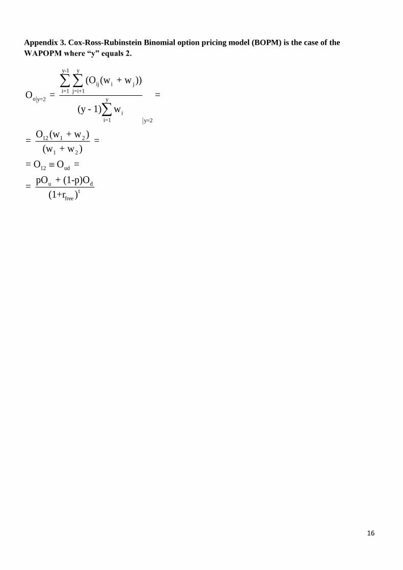
Appendix 3. Cox-Ross-Rubinstein Binomial option pricing model (BOPM) is the case of the

WAPOPM where “y” equals 2.

y-1 y

ij i j

i=1 j=i+1

o y=2 y

i

i=1 y=2

12 1 2

1 2

12 ud

u d

t

free

(O (w + w ))

O = =

(y - 1) w

O (w + w )= =

(w + w )

= O O =

pO + (1-p)O=

(1+r )

valuing innovation-based investments with the … · 2/4/2017 · valuing innovation-based...

Documents