valuing flexibility: the case of an integrated

VALUING FLEXIBILITY: THE CASE OF AN INTEGRATED GASIFICATION COMBINED

CYCLE POWER PLANT

by

Luis M. Abadie and José M. Chamorro

2005

Working Paper Series: IL. 21/05

Departamento de Fundamentos del Análisis Económico I

Ekonomi Analisiaren Oinarriak I Saila

University of the Basque Country

Valuing Flexibility: The case of an Integrated

Gasification Combined Cycle Power Plant∗

Luis M. AbadieBilbao Bizkaia Kutxa

Gran Vıa, 3048009 Bilbao, SpainTel +34-607408748Fax +34-944017996

E-mail: [email protected]

Jose M. ChamorroUniversity of the Basque Country

Dpt. Fundamentos del Analisis Economico IAv. Lehendakari Aguirre, 83

48015 Bilbao, SpainTel. +34-946013769Fax +34-946013891

E-mail: [email protected]

October 17th 2005

JEL Codes: C6, E2, D8, G3.

∗We would like to thank seminar participants at the 9th Conference on Real Options(Paris 2005) for their helpful comments. We remain responsible for any errors. Chamorroacknowledges financial support from research grant 9/UPV00I01.I01-14548/2002.

1

2

Abstract

In this paper we analyze the valuation of options stemming fromthe flexibility in an Integrated Gasification Combined Cycle (IGCC)Power Plant.

First we use as a base case the opportunity to invest in a NaturalGas Combined Cycle (NGCC) Power Plant, deriving the optimalinvestment rule as a function of fuel price and the remaining life of theright to invest. Additionally, the analytical solution for a perpetualoption is obtained.

Second, the valuation of an operating IGCC Power Plant isstudied, with switching costs between states and a choice of the bestoperation mode. The valuation of this plant serves as a base to obtainthe value of the option to delay an investment of this type.

Finally, we derive the value of an opportunity to invest eitherin a NGCC or IGCC Power Plant, that is, to choose between aninflexible and a flexible technology, respectively.

Numerical computations involve the use of one- and two-dimensionalbinomial lattices that support a mean-reverting process for the fuelprices. Basic parameter values refer to an actual IGCC power plantcurrently in operation.

Keywords: Real options, Power plants, Flexibility, StochasticCosts.

1 INTRODUCTION 3

1 Introduction

It is broadly accepted in the financial literature that the traditional valuationtechniques based on discounted cash flows are not the most appropriate toolfor evaluating uncertain investments, especially in presence of irreversibilityconsiderations, or a chance to defer investment, or when there is scope forflexible management. In these cases, it is usually preferable to employ themethods for pricing options, such as Contingent Claims Analysis or DynamicProgramming.

On the other hand, the energy sector is of paramount importance forthe development of any society. Besides, its specific weight both in the realand financial sectors of the economy cannot be neglected. Therefore the useof inadequate instruments in decision making may be particularly onerous.In addition, the high sums involved in the energy industry, its operatingflexibility and environmental impact, the progressive liberalization of themarkets for its inputs and outputs along with many types of uncertainties,all of them render this kind of investments a suitable candidate to be valuedas real options.

The aim of this paper is to use the real options methodology to assessdecisions of investment in power plants. In particular, our firm is goingto decide simultaneously the time to invest and the choice of technology.Specifically, we compare an inflexible technology (Natural Gas CombinedCycle, or NGCC henceforth) with a flexible one (Integrated GasificationCombined Cycle, or IGCC). We derive the best mode of operation, thevalue of the investments and the optimal investment rule when there isan option to wait. We consider two mean-reverting stochastic processes forcoal and natural gas prices, both of the Inhomogeneous Geometric BrownianMotion (IGBM) type, and also switching costs between modes of operation.The output (electricity) price, though, follows a deterministic path. Basicparameter values in our computations refer to an actual IGCC power plantcurrently in operation.

From a growing strand of related literature we would mention Herbelot[7], who studied the fulfillment of restrictions on SO2 emissions, eitherthrough the purchase of emission permits, or changing the fuel or deletingpolluting agents in the factory itself.1 On the other hand, Kulatilaka [10]developes a dynamic model that allows to value the flexibility in a flexiblemanufacturing system with several modes of operation, using a matrix oftransition probabilities between states. In this paper, the importance offlexibility in the design of systems from the viewpoint of both engineersand competitors is emphasized. Later on, Kulatilaka [12] analyzes thechoice between a flexible technology (fired by oil or gas) and two inflexibletechnologies to generate electricity. Some numerical results appear in

1A brief summary of this work appears in Dixit and Pindyck [6].

2 THE NGCC AND IGCC TECHNOLOGIES 4

Kulatilaka [11], where he normalizes the gas price in terms of the oil price.A similar problem with two stochastic processes is dealt with in Brekke andSchieldrop [3], but in this case there are no switching costs while pricesfollow standard geometric brownian motions. Finally, Robel [14] and Insley[8] develop some aspects of the stochastic process that we have adopted.

The paper is organized as follows. In Section 2 we briefly introduce theIGCC and NGCC technologies. Section 3 presents the stochastic model forfuel price (IGBM), its main features and the binomial lattices for one andtwo variables that we use later in the numerical applications. 2 Also in thissection, the differential equations for the value of a power plant and that foran option to invest in it are derived. In particular, we focus on a perpetualoption to invest in an asset whose value depends on fuel price. We obtaina solution in terms of Kummer’s confluent hypergeometric function. Theresults serve later on to verify how the binomial lattices behave. In Section4 first we report some basic parameter values from an actual power plantthat we use in our computations. Then we value an operating NGCC plantand the option to invest in it. We also value an operating IGCC plant withswitching costs and the right to invest in this flexible technology. Finally wederive the optimal investment rule when it is possible to choose between theNGCC and IGCC alternatives. A section with our main findings concludes.

2 The NGCC and IGCC technologies

2.1 Some features of electric power plants

The production of electricity can be viewed as the exercise of a series ofnested real options to transform a type of energy (gas, oil, coal, or other)into electric energy. There are two sets of outstanding information. Thefirst one has to do with the characteristics of the energy inputs used in theproduction process. The second one comprises the operation features of theelectric power plants, among them: the net output, the rate of efficiency(“operating heat rate”), the costs to start and stop, the fixed costs, thestarting and stopping periods, and the physical restrictions that preventinstantaneous changes between states. These factors determine the wedgebetween the prices of the energy consumed and produced. On this basis, ateach instant it is necessary to decide how much electricity to produce andhow, i.e. the possible state changes to realize.

2The choice of the binomial lattice as a resolution method is due both to its suitabilityand acceptance by the industry. See Mun [13].


2.2 Natural Gas Combined Cycle (NGCC) Technology

It is based on the employment of two turbines, one of natural gas and anotherone of steam.3 The exhaust gases from the first one are used to generate thesteam that is used in the second turbine. Thus it consists of a Gas-Air cycleand a Water-Steam cycle. This system allows for a higher net efficiency, 4

close to 55%; future trends aim at reaching net efficiencies of 60% in NGCCplants of 500 Mw.

The advantages of a NGCC Power Plant are:5

• a) Lower emissions of CO2, estimated about 350 g/Kwh, which allowan easier fulfillment of the Kyoto protocol;

• b) Higher net efficiency, between 50% and 60%;

• c) Low cost of the investment, about 500 AC/Kw installed;

• d) Less consumption of water and space requirements, which allow tobuild in a shorter period of time and closer to consumer sites;

• e) Lower operation costs, with typical values of 0.35 cents AC/KWh.

In addition, a NGCC power plant can be designed as a base plant oras a peak plant; in the latter case, it only operates when electricity pricesare high enough, what usually happens during periods of strong growth indemand.

On the other hand, the disadvantages of a NGCC Power Plant are:

• a) The higher cost of the natural gas fired in relation to coal’s;

• b) The insecurity concerning gas supplies, since reserves are moreunevenly distributed over the world;

• c) The strong rise in the demand for natural gas, which can cause aconsolidation of prices at higher than historical levels.

2.3 Integrated Gasification Combined Cycle (IGCC)Technology

It is based on the transformation of coal into synthesis gas, which iscomposed principally of carbon monoxide (CO) and hydrogen (H2).6 This

3Also known as Combined Cycle Gas Turbines or CCGT.4The net efficiency refers to the percentage of the heating value of the fuel that is

transformed into electric energy.5Our reference is ELCOGAS (2003): “Integrated gasification combined cycle

technology: IGCC” and its actual application at the power plant in Puertollano (Spain).6According to the following reactions: C + CO2 → 2 CO and C + H2O → CO + H2.


gas keeps approximately 90% of the heating value of the original coal.However, the appearance of CO as a by-product demands a special carewith this technology, given the harmful impact of small quantities of thisgas on human health. Besides, the process of gasification increases the costsof the original investment and those of operating a plant of this type.

The synthesis gas obtained has several applications:

• a) Generation of electric energy in IGCC power plants;

• b) Production of hydrogen for diverse uses, like fuel cells; note thepromising future of hydrogen as a fuel in general;

• c) As an input to chemical products, like ammonia, for manufacturingfertilizers;

• d) As an input to produce sulphur and sulphuric acid.

After the stage of gasification, it is time to clean the gas by meansof washing processes with water and absorption with dissolvents. Thismakes it possible that an IGCC plant has significantly lower emissions ofSO2, NOx and particles, in relation to those generated in standard coalpower plants. The emissions of CO2 per Kwh are also lower, but in thiscase the improvement derives mainly from the higher net efficiency of thecycle (currently, typical values fluctuate around 42%, whith a trend towardsapproaching 50%, provided this methodology enhances its design, which isin its first steps). Right now, the emissions of CO2 from an IGCC powerplant (about 725 g/Kwh ) are estimated at 20% lower than those from aclassic coal power plant 7. However, they are clearly higher than those fromNGCC (around 350 g/Kwh ).

In addition to the gasification plant, the operation of an IGCC powerplant requires another costly element, namely the air separation unit, forproducing oxygen as an oxidizing agent. This unit may represent between10% and 15% of total investment. Needless to say, the units for gasification,air separation, and other auxiliary systems raise the initial outlay and implyhigher operation costs.

From the viewpoint of real options, it is necessary to highlight thefollowing aspects of this technology:

• a) The investment in an IGCC plant can be considered as a strategicinvestment in a new technology, whose ultimate results will depend onits final success or failure;

7Coal power plants are classified in subcritical, supercritical and ultrasupercritical,depending on the pressure and the temperature of the steam. The net efficiency for coalpower plants rounds about 35% in the supercriticals, and increases with higher investmentcosts but also entails an increased hazard due to working at higher temperatures.

3 THE STOCHASTIC MODEL FOR THE FUEL PRICE 7

• b) The IGCC power plant is a flexible technology concerning thepossible fuels to use; apart from the synthesis gas, it may fire oilcoke, heavy refinery liquid fuels, natural gas, biomasss, and urbansolid waste, among others. In this way, at each time it is possible tochoose the best input combination according to relative prices. Thevaluation of this operating flexibility between synthesis gas and naturalgas constitutes one of the aims of this paper.

3 The stochastic model for the fuel price

3.1 The Inhomogeneous Geometric Brownian Motion(IGBM)

In a model for long-term valuation of energy assets, it is convenient to keepin mind that prices tend to revert towards levels of equilibrium after anincidental change. Among the models with mean reversion, we have chosenthe Integrated or Inhomogeneous Geometric Brownian Motion or IGBMprocess (Bhattacharya [2], Sarkar [15]):

dSt = k(Sm − St)dt + σStdZt, (1)

where:St: the price of fuel at time t.Sm: the level fuel price tends to in the long run.k: the speed of reversion towards the “normal” level. It can be computed

as k = log 2/t1/2, where t1/2 is the expected half-life, that is the time for thegap between St and Sm to halve.

σ: the instantaneous volatility of fuel price, which determines thevariance of St at t.

dZt: the increment to a standard Wiener process. It is normallydistributed with mean zero and variance dt.

Some of the reasons for our choice are:

• a) This model satisfies the following condition (which seemsreasonable): if the price of one unit of fuel reverts to some mean value,then the price of two units reverts to twice that same mean value.

• b) The term σStdZt in the differential equation precludes, almostsurely, the possibility of negative values.

• c) This model admits as a particular solution dSt = αStdt + σStdZt

when Sm = 0 and α = −k; therefore it includes Geometric BrownianMotion (GBM) as a particular case.

• d) The expected value in the long run is: E(S∞) = Sm; this is not

true in Schwartz [16], where E(S∞) = Sm(e−σ2

4k ).


3.1.1 First and second moments of the actual process

Now we compute the first two moments of an actual path described by anIGBM process.8Following Kloeden and Platen [9],9 for a linear stochasticdifferential equation of the form:

dXt = (a1(t)Xt + a2(t))dt + (b1(t)Xt + b2(t))dWt, (2)

and denoting m(t) ≡ E(St) and P (t) ≡ E(S2t ), we have:

dm(t)dt

= a1(t)m(t) + a2(t), (3)

dP (t)dt

= (2a1(t) + b21(t))P (t) + 2m(t)(a2(t) + b1(t)b2(t)) + b2

2(t). (4)

For our IGBM process, a1 = −k, a2 = kSm, b1 = σ and b2 = 0.

A) Expected value.In this case, the expected value satisfies the following differential

equation:dm(t)

dt= −km(t) + kSm = k(Sm −m(t)). (5)

This equation can be easily integrated:

E(St) ≡ m(t) = Sm + (S0 − Sm)e−kt, (6)

where S0 stands for current price. As mentioned above, when t → ∞ theexpected value is E(S∞) = Sm.10

B) Second non-central moment.For the second non-central moment of an IGBM process, the ordinary

differential equation is:

dP (t)dt

= (−2k + σ2)P (t) + 2m(t)kSm. (7)

After substituting and rearranging, this can be rewritten as:

dP (t)dt

+ (2k − σ2)P (t) = 2kSm

(Sm + (S0 − Sm)e−kt

). (8)

Using an integration factor µ = e(2k−σ2)t:

µP (t) = 2kSm

∫ t

0e(2k−σ2)t

(Sm + (S0 − Sm)e−kt

)dt + c. (9)

8The actual path obeys the real trend. Consequently it cannot be used for risk-neutralvaluation.

9Equations (2.10) and (2.11) in page 113.10It can be verified that when k = −α and Sm = 0, the expected value of the GBM

model results: E(St) = S0eαt.


After some algebra:

P (t) ≡ E(S2t ) =

2kS2m

2k − σ2(1−e(σ2−2k)t)+

2kSm(S0 − Sm)k − σ2

(e−kt−e(σ2−2k)t)+

+S20e(σ2−2k)t, (10)

where we have substituted S20 for the constant c so that in t = 0 the moment

takes on the value S20 .

There are two especial situations, both highly unlikely in practice. Theyinvolve cases in which denominators are zero or indeterminacies like 0

0appear:

• a) k = σ2

2 . In this case, applying L’Hospital rule, P (t) simplifies to:

P (t) = 2kS2mt + 2Sm(Sm − S0)(e−kt − 1) + S2

0 . (11)

• b) k = σ2. In this case, the solution reduces to:

P (t) = 2S2m(1− e−kt)− 2kSm(Sm − S0)te−kt + S2

oe−kt. (12)

Now, from the formula for the second non-central moment, we can derivethe explicit solution for the variance:

V ar(St) = E((St − E(St))2

)=

= e(σ2−2k)t

(S2

0 +2kS2

m

σ2 − 2k+

2kSm(S0 − Sm)σ2 − k

)+

+e−kt(

2kSm(S0 − Sm)k − σ2

+ 2Sm(Sm − S0))−e−2kt(S0−Sm)2+

2kS2m

2k − σ2−S2

m.

(13)

In particular, when 2k > σ2 and t →∞, the variance tends to:

2kS2m

2k − σ2− S2

m. (14)

Only when the speed of reversion k is sufficiently high in relation to σ2,the variance converges towards a finite value. Otherwise the variance growswithout limit with the passage of time.11

Finally, in subsequent sections it will be convenient to use simplerexpressions for the numerical computations. It is known that when theincrement ∆t is very small, given eat = 1 + at + (at)2

2 + . . . , then ea∆t ≈1 + a∆t. Substituting in expressions (6) and (13), the usual results ofEuler-Maruyama’s approximation arise:

E(St) ≈ St−1 + k(Sm − St−1)∆t, (15)

V ar(St) ≈ σ2S2t−1∆t. (16)

11When Sm = 0 and k = −α, we get: V ar(St) = S20e(σ2+2α)t−S2

0e2αt = S20e2αt(eσ2t−1).

That is, we get the formula corresponding to a standard GBM process.


3.2 The Risk-Neutral IGBM Process

When using binomial lattices below, we will make use of the risk-neutralvaluation principle.

3.2.1 The fundamental pricing equation

The change from an actual process to a risk-neutral one is accomplished byreplacing the drift in the price process (in the GBM case, α) with the growthrate in a risk-neutral world (r − δ, where r is the riskless interest rate andδ denotes the net convenience yield). Note, though, that the convenienceyield is not constant in a mean-reverting process .12

In order to obtain the risk-neutral version of the IGBM process, wesimply discount a risk premium (which, according to the CAPM, is)

ρσφS (17)

to its actual rate of growth. In this expression, ρ is the correlation betweenthe returns on the market portfolio and the fuel asset, and σ is the asset’svolatility. Finally, φ denotes the market price of risk, which is defined as:

φ ≡ rM − r

σM, (18)

where rM is the expected return on the market portfolio and σM denotes itsvolatility.

If certain ”complete market” assumptions hold, it can be shown that thevalue of an investment V (S, t), which is a function of fuel price and calendartime, follows the differential equation:

12σ2S2 ∂2V

∂S2+ [k(Sm − S)− ρσφS]

∂V

∂S+

∂V

∂t− rV + C(S, t) = 0, (19)

where C(S, t) is the instantaneous cash flow generated by the investment.

3.2.2 First and second moments of the risk-neutral process

Let St denote the risk-neutral version of St:

dSt = [k(Sm − St)− ρσφSt]dt + σStdZt. (20)

Then it can be shown that it has an expected value:

E(St) =kSm

k + ρσφ[1− e−(k+ρσφ)t] + S0e

−(k+ρσφ)t. (21)

12If we equate (r− δ)St to the difference between the coefficient of dt in (1) and the riskpremium, the resulting expression for δ is a function of St.


Using the first two elements of a Taylor expansion, this can be approximatedby:

E(St) ≈ St−1 + (kSm − St−1(k + ρσφ))∆t. (22)

Concerning the second non-central moment, it is:

E(S2t ) =

2k2S2m

(k + ρσφ)(1− e−(2k+2ρσφ−σ2)t)

(2k + 2ρσφ− σ2)−

− 2k2S2m

(k + ρσφ)(e−(k+ρσφ)t − e−(2k+2ρσφ−σ2)t)

(k + ρσφ− σ2)+

+2kSmS0(e−(k+ρσφ)t − e−(2k+2ρσφ−σ2)t)

(k + ρσφ− σ2)+ S2

0e−(2k+2ρσφ−σ2)t. (23)

After discretization, there results: V ar(St) ≈ σ2S2t−1∆t.

3.3 Binomial Lattice for a risk-neutral IGBM variable

The time horizon T is subdivided in n steps, each of size ∆t = T/n. Startingfrom an initial value S0, at time i, after j positive increments, the value ofthe fuel asset is given by S0u

jdi−j , where d = 1/u.Consider an asset whose risk-neutral behaviour follows the differential

equation:dS = (k(Sm − S)− ρσφS)dt + σSdZ. (24)

This can also be written as:

dS =

(k(Sm − S)

S− ρσφ

)Sdt + σSdZ = µSdt + σSdZ. (25)

Since it is usually easier to work with the processes for the natural logarithmsof asset prices, we carry out the following transformation: X = lnS. ThusXs = 1/S, Xss = −1/S2, Xt = 0, and by Ito’s Lemma:

dX = (k(Sm − S)

S− ρσφ− 1

2σ2)dt + σdZ = µdt + σdZ, (26)

where µ ≡ k(Sm − S)/S − ρσφ− 12σ2 depends at each moment on the asset

value S.Following Euler-Maruyama’s discretization, the probabilities of upward

and downward movements must satisfy three conditions:

• a) pu + pd = 1.

• b) E(∆X) = pu∆X − pd∆X =(

k(Sm−S)

S− ρσφ− 1

2σ2

)∆t = µ∆t.

The aim is to equate the first moment of the binomial lattice (pu∆X−pd∆X) to the first moment of the risk-neutral underlying variable(µ∆t).


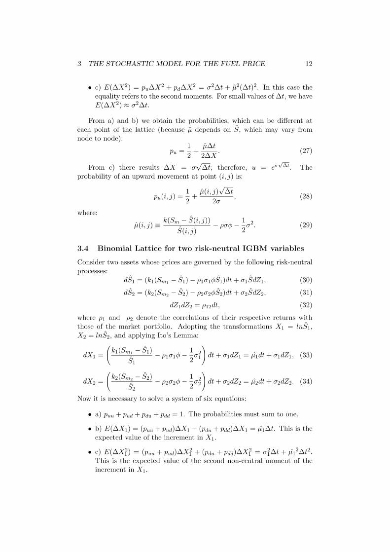
• c) E(∆X2) = pu∆X2 + pd∆X2 = σ2∆t + µ2(∆t)2. In this case theequality refers to the second moments. For small values of ∆t, we haveE(∆X2) ≈ σ2∆t.

From a) and b) we obtain the probabilities, which can be different ateach point of the lattice (because µ depends on S, which may vary fromnode to node):

pu =12

+µ∆t

2∆X. (27)

From c) there results ∆X = σ√

∆t; therefore, u = eσ√

∆t. Theprobability of an upward movement at point (i, j) is:

pu(i, j) =12

+µ(i, j)

√∆t

2σ, (28)

where:

µ(i, j) ≡ k(Sm − S(i, j))S(i, j)

− ρσφ− 12σ2. (29)

3.4 Binomial Lattice for two risk-neutral IGBM variables

Consider two assets whose prices are governed by the following risk-neutralprocesses:

dS1 = (k1(Sm1 − S1)− ρ1σ1φS1)dt + σ1SdZ1, (30)

dS2 = (k2(Sm2 − S2)− ρ2σ2φS2)dt + σ2SdZ2, (31)

dZ1dZ2 = ρ12dt, (32)

where ρ1 and ρ2 denote the correlations of their respective returns withthose of the market portfolio. Adopting the transformations X1 = lnS1,X2 = lnS2, and applying Ito’s Lemma:

dX1 =

(k1(Sm1 − S1)

S1

− ρ1σ1φ−12σ2

1

)dt + σ1dZ1 = µ1dt + σ1dZ1, (33)

dX2 =

(k2(Sm2 − S2)

S2

− ρ2σ2φ−12σ2

2

)dt + σ2dZ2 = µ2dt + σ2dZ2. (34)

Now it is necessary to solve a system of six equations:

• a) puu + pud + pdu + pdd = 1. The probabilities must sum to one.

• b) E(∆X1) = (puu + pud)∆X1 − (pdu + pdd)∆X1 = µ1∆t. This is theexpected value of the increment in X1.

• c) E(∆X21 ) = (puu + pud)∆X2

1 + (pdu + pdd)∆X21 = σ2

1∆t + µ12∆t2.

This is the expected value of the second non-central moment of theincrement in X1.


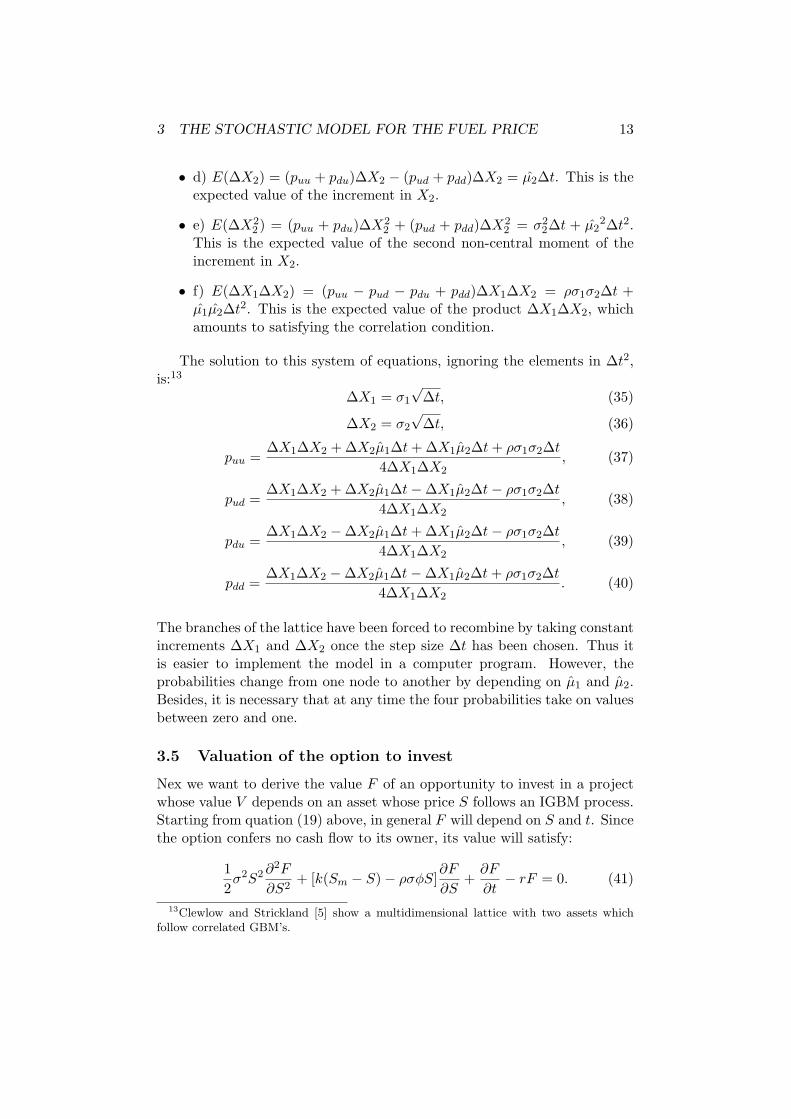
• d) E(∆X2) = (puu + pdu)∆X2 − (pud + pdd)∆X2 = µ2∆t. This is theexpected value of the increment in X2.

• e) E(∆X22 ) = (puu + pdu)∆X2

2 + (pud + pdd)∆X22 = σ2

2∆t + µ22∆t2.

This is the expected value of the second non-central moment of theincrement in X2.

• f) E(∆X1∆X2) = (puu − pud − pdu + pdd)∆X1∆X2 = ρσ1σ2∆t +µ1µ2∆t2. This is the expected value of the product ∆X1∆X2, whichamounts to satisfying the correlation condition.

The solution to this system of equations, ignoring the elements in ∆t2,is:13

∆X1 = σ1

√∆t, (35)

∆X2 = σ2

√∆t, (36)

puu =∆X1∆X2 + ∆X2µ1∆t + ∆X1µ2∆t + ρσ1σ2∆t

4∆X1∆X2, (37)

pud =∆X1∆X2 + ∆X2µ1∆t−∆X1µ2∆t− ρσ1σ2∆t

4∆X1∆X2, (38)

pdu =∆X1∆X2 −∆X2µ1∆t + ∆X1µ2∆t− ρσ1σ2∆t

4∆X1∆X2, (39)

pdd =∆X1∆X2 −∆X2µ1∆t−∆X1µ2∆t + ρσ1σ2∆t

4∆X1∆X2. (40)

The branches of the lattice have been forced to recombine by taking constantincrements ∆X1 and ∆X2 once the step size ∆t has been chosen. Thus itis easier to implement the model in a computer program. However, theprobabilities change from one node to another by depending on µ1 and µ2.Besides, it is necessary that at any time the four probabilities take on valuesbetween zero and one.

3.5 Valuation of the option to invest

Nex we want to derive the value F of an opportunity to invest in a projectwhose value V depends on an asset whose price S follows an IGBM process.Starting from quation (19) above, in general F will depend on S and t. Sincethe option confers no cash flow to its owner, its value will satisfy:

12σ2S2 ∂2F

∂S2+ [k(Sm − S)− ρσφS]

∂F

∂S+

∂F

∂t− rF = 0. (41)

13Clewlow and Strickland [5] show a multidimensional lattice with two assets whichfollow correlated GBM’s.


3.5.1 Analytical Solution of the perpetual investment option

Let F be the value of a perpetual call option on an investment V which inturn depends on the value of an asset S following an IGBM process. In thiscase, the term Fτ disappears in (41):

12Fssσ

2S2 + (k(Sm − S)− ρσφS)Fs − rF = 0. (42)

This equation may be rewritten as:

FssS2 + (αS + β)Fs − γF = 0, (43)

where the following notation has been adopted:

α = −2(k + ρσφ)σ2

,

β =2kSm

σ2,

γ =2r

σ2.

In order to find a solution to this equation, we define a function h(βS−1) by

F (S) = A0(βS−1)θh(βS−1). (44)

where A0 and θ are constants that will be chosen so as to make h(•) satisfy adifferential equation with a known solution. The first and second derivatives,divided by A0β

θ, are:

FS(S)A0βθ

= (−θ)S−θ−1h(βS−1) + S−θ−2h′(βS−1)(−β),

FSS(S)A0βθ

= θ(θ + 1)S−θ−2h(βS−1) + (−θ)S−θ−3h′(βS−1)(−β) +

+S−θ−3(−θ − 2)(−β)h′(βS−1) + S−θ−4h

′′(βS−1)β2.

Substituting these expressions in (43) and simplifying we get:

S−θh(βS−1) (θ(θ + 1)− αθ − γ) + S−θ−1(S−1β2h

′′(βS−1) +

+h′(βS−1)(βθ + (θ + 2)β − αβ − S−1β2)− h(βS−1)θβ)

= 0

For this equality to hold, first it must be:

θ(θ + 1)− θα− γ = θ2 + θ(1− α)− γ = 0. (45)


This equation allows to determine the positive value of θ, since the remainingterms are known constants.

Once the value of θ has been obtained, the remainder of the equation is:

(βS−1)h′′(βS−1) + h

′(βS−1)(2θ + 2− α− βS−1)− θh(βS−1) = 0.

This is Kummer’s Differential Equation, 14 where: a = θ, b = 2θ + 2 − α,and z = (βS−1). The general solution to this equation has the form:

h(βS−1) = A1U(a, b, z) + A2M(a, b, z), (46)

where U(a, b, z) is Tricomi’s or second-order hypergeometric function, andM(a, b, z) is Kummer’s or first-order hypergeometric function.

Therefore, the general solution to (44) will be:

F (S) = A0(βS−1)θ(A1U(a, b, z) + A2M(a, b, z)). (47)

The second-order hypergeometric function has the following representation:

U(a, b, z) =Γ(1− b)

Γ(1 + a− b)M(a, b, z) +

Γ(b− 1)Γ(a)z(b−1)

M(1 + a− b, 2− b, z), (48)

where Γ(.) is the gamma function and M(a,b,z) is Kummer’s function, whosevalue is given by:

M(a, b, z) = 1 +a

bz +

a(a + 1)b(b + 1)

z2

2!+

a(a + 1)(a + 2)b(b + 1)(b + 2)

z3

3!+ . . . (49)

The derivatives of Kummer’s function have the following properties:

∂M(a, b, z)∂z

=a

bM(a + 1, b + 1, z),

∂2M(a, b, z)∂z2

=a(a + 1)b(b + 1)

M(a + 2, b + 2, z).

The derivatives of Tricomi’s function satisfy:

∂U(a, b, z)∂z

= −aU(a + 1, b + 1, z),

∂2U(a, b, z)∂z2

= a(a + 1)U(a + 2, b + 2, z).

14See Abramowitz and Stegun [1], equation 13.1.1.

4 VALUATION OF ALTERNATIVE TECHNOLOGIES 16

The boundary conditions will determine whether A1 or A2 in (47) are zero.In our case, S refers to a fuel, so we face stochastic costs. An upwardevolution in S entails a reduction in profits, so F (∞) = 0 and z = 0, thenA1 = 0 and the term in Kummer’s function remains.15 The solution is:

F (S) = Am(βS−1)θM(a, b, z), (50)

with Am ≡ A0A2.16

The constant Am and the critical value S∗ below which it is optimal toinvest must be jointly determined by the remaining two boundary conditions:

• Value-Matching: F (S∗) = V (S∗)− I(S∗),

• Smooth-Pasting: FS(S∗) = VS(S∗)− IS(S∗).

4 Valuation of alternative technologies

4.1 Representative values used in the numerical applications

We have used the standard values that appear in Table 1 (ELCOGAS, 2003).

Table 1. Basic parametersConcepts Coal Plant IGCC NGCC Base

Plant Size Mw (P) 500 500 500Production Factor (%) (FP) 80% 80% 80%Net Efficiency (%) (RDTO) 35% 41% 50.5%

Unit Investment Cost AC/Kw (i) 1,186 1,300 496O&M cts. AC/Kwh (CVAR) 0.68 0.71 0.32

The Production Factor is the percentage of the total capacity used onaverage over the year. Using these data, the heat rate, the plant’sconsumption of energy, and the total production of electricity can becomputed:

Heat Rate: HR = 3600/RDTO/1, 000, 000, in GJ/Kwh.17

Investment Cost I = 1000 ∗ i ∗ P , in Euros.18

Total annual production: A = 1000 ∗ P ∗ 365 ∗ 24 ∗ FP , in Kwh.Fuel energy needs: B = 1000 ∗ P ∗ 365 ∗ 24 ∗ FP ∗HR, in GJ/year.Now with these formula we estimate the parameters in Table 2.

15Due to the fact that U(a, b, 0) = ∞ if b > 1; this will be shown to hold with ourparameter values below.

16When a downward evolution of S entails a reduction in profits, so that F (0) = 0and z = ∞, then A2 = 0 and the term in Tricomi’s function remains. The solution isAu(βS−1)θU(a, b, z) with Au ≡ A0A1, since M(a, b,∞) =∞ and then it must be A2 = 0.This would be the case of stochastic revenues.

17One Kwh amounts to 3,600 KJ, and a GJ (Gigajoules) is a million KJ (Kilojoules).18Since power is measured in Mw.


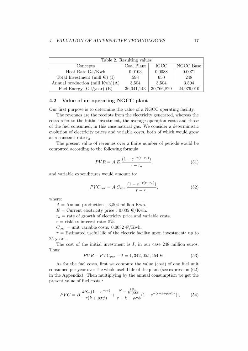
Table 2. Resulting valuesConcepts Coal Plant IGCC NGCC Base

Heat Rate GJ/Kwh 0.0103 0.0088 0.0071Total Investment (mill AC) (I) 593 650 248

Annual production (mill Kwh)(A) 3,504 3,504 3,504Fuel Energy (GJ/year) (B) 36,041,143 30,766,829 24,979,010

4.2 Value of an operating NGCC plant

Our first purpose is to determine the value of a NGCC operating facility.The revenues are the receipts from the electricity generated, whereas the

costs refer to the initial investment, the average operation costs and thoseof the fuel consumed, in this case natural gas. We consider a deterministicevolution of electricity prices and variable costs, both of which would growat a constant rate ra.

The present value of revenues over a finite number of periods would becomputed according to the following formula:

PV R = A.E.(1− e−τ(r−ra))

r − ra, (51)

and variable expenditures would amount to:

PV Cvar = A.Cvar.(1− e−τ(r−ra))

r − ra, (52)

where:A = Annual production : 3,504 million Kwh.E = Current electricity price : 0.035 AC/Kwh.ra = rate of growth of electricity price and variable costs.r = riskless interest rate: 5%.Cvar = unit variable costs: 0.0032 AC/Kwh.τ = Estimated useful life of the electric facility upon investment: up to

25 years.The cost of the initial investment is I, in our case 248 million euros.

Thus:PV R− PV Cvar − I = 1, 342, 055, 454 AC. (53)

As for the fuel costs, first we compute the value (cost) of one fuel unitconsumed per year over the whole useful life of the plant (see expression (62)in the Appendix). Then multiplying by the annual consumption we get thepresent value of fuel costs :

PV C = B[kSm(1− e−rτ)

r(k + ρσφ)+

S − kSmk+ρσφ

r + k + ρσφ(1− e−(r+k+ρσφ)τ )], (54)


where B is the annual fuel energy needed in GJ and S stands for thenatural gas price. Assuming the additional values: Sm = 3.25 AC/GJ, ρ = 0,φ = 0.40, k = 0.25, σ = 0.20 and substituting them in the above formulawe obtain the average cost per unit consumed yearly during the facility’slife: 35.5498 + 3.3315S. Now multiplying the annual unit cost by annualconsumption (B in Table 2) we get 887, 999, 971 + 83, 217, 315S. For thespecific value S = 5.45 AC/GJ, we finally compute:

NPV (NGCC) = PV R− PV Cvar − I − PV C = 521, 120AC. (55)

4.3 Valuation of the opportunity to invest in a NGCC plant

4.3.1 The perpetual option

Consider the case of a NGCC plant described by the last column in Table 1.As already seen, the present value of revenues minus the investment outlayand the present value of variable costs amounts to 1, 342, 055, 454 AC, whereasthe present value of fuel costs is 887, 999, 971+83, 217, 315S. Thus the valueof the investment if realized now is: V (S)−I = 454, 055, 483−83, 217, 315S.

In this case, the boundary conditions would be:

• Value-Matching: F (S∗) = Am(β(S∗)−1)θM(a, b, β(S∗)−1) =454,055,483-83,217,315S∗ = V (S∗)− I(S∗)

• Smooth-Pasting: FS(S∗) =Am(β(S∗)−1)θ( − θ(S∗)−1M(a, b, β(S∗)−1) − aβ

b(S∗)2 M(a + 1, b +1, β(S∗)−1)) = −83, 217, 315 = VS(S∗)− IS(S∗)

By computing α = −12.5, β = 40.625, γ = 2.5, and θ = 0.1827, wederive a and b: a = 0.1827, b = 14.8654.

Thus we have a system of two equations that will allow us to determineAm and S∗. Substituting the value Am(β(S∗)−1)θ, from the Value-Matchingcondition, in the Smooth-Pasting condition, there results an equation in S∗

which has as its solution S∗ = 2.7448.Next it is easy to determine that Am = 94, 394, 000 and, finally, that the

value of the option for a gas price S is:

F (S) = 94, 394, 000 ∗ (40.625

S)0.1827M(0.1827, 14.8654,

40.625S

)

In our case, with S = 5.45, initially the option value is 153, 870, 000 AC,against a NPV = 521, 120 AC; thus it is optimal to wait.

If there were no other option but to invest now or never, the hurdlepoint would be V (S∗∗) = I(S∗∗), whence we get S∗∗ = 5.4563. However,with a perpetual option it is preferable to wait, since in principle and inthe long run natural gas price is going to decrease and fluctuate around a


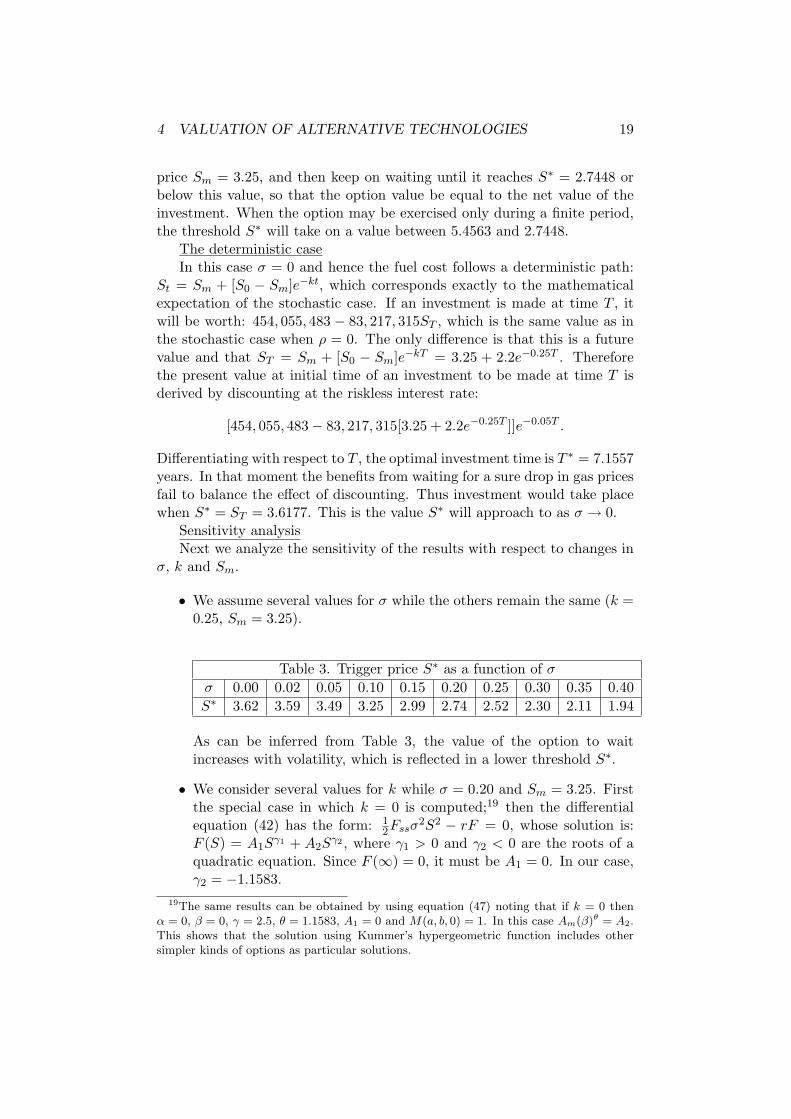
price Sm = 3.25, and then keep on waiting until it reaches S∗ = 2.7448 orbelow this value, so that the option value be equal to the net value of theinvestment. When the option may be exercised only during a finite period,the threshold S∗ will take on a value between 5.4563 and 2.7448.

The deterministic caseIn this case σ = 0 and hence the fuel cost follows a deterministic path:

St = Sm + [S0 − Sm]e−kt, which corresponds exactly to the mathematicalexpectation of the stochastic case. If an investment is made at time T , itwill be worth: 454, 055, 483 − 83, 217, 315ST , which is the same value as inthe stochastic case when ρ = 0. The only difference is that this is a futurevalue and that ST = Sm + [S0 − Sm]e−kT = 3.25 + 2.2e−0.25T . Thereforethe present value at initial time of an investment to be made at time T isderived by discounting at the riskless interest rate:

[454, 055, 483− 83, 217, 315[3.25 + 2.2e−0.25T ]]e−0.05T .

Differentiating with respect to T , the optimal investment time is T ∗ = 7.1557years. In that moment the benefits from waiting for a sure drop in gas pricesfail to balance the effect of discounting. Thus investment would take placewhen S∗ = ST = 3.6177. This is the value S∗ will approach to as σ → 0.

Sensitivity analysisNext we analyze the sensitivity of the results with respect to changes in

σ, k and Sm.

• We assume several values for σ while the others remain the same (k =0.25, Sm = 3.25).

Table 3. Trigger price S∗ as a function of σ

σ 0.00 0.02 0.05 0.10 0.15 0.20 0.25 0.30 0.35 0.40S∗ 3.62 3.59 3.49 3.25 2.99 2.74 2.52 2.30 2.11 1.94

As can be inferred from Table 3, the value of the option to waitincreases with volatility, which is reflected in a lower threshold S∗.

• We consider several values for k while σ = 0.20 and Sm = 3.25. Firstthe special case in which k = 0 is computed;19 then the differentialequation (42) has the form: 1

2Fssσ2S2 − rF = 0, whose solution is:

F (S) = A1Sγ1 + A2S

γ2 , where γ1 > 0 and γ2 < 0 are the roots of aquadratic equation. Since F (∞) = 0, it must be A1 = 0. In our case,γ2 = −1.1583.

19The same results can be obtained by using equation (47) noting that if k = 0 thenα = 0, β = 0, γ = 2.5, θ = 1.1583, A1 = 0 and M(a, b, 0) = 1. In this case Am(β)θ = A2.This shows that the solution using Kummer’s hypergeometric function includes othersimpler kinds of options as particular solutions.


The boundary conditions are:

Value-Matching: A2(S∗)γ2 = 1, 342, 055, 454− 356, 448, 075S∗,

Smooth-Pasting: A2γ2(S∗)γ2−1 = −356, 448, 075.

They suffice to determine the value of S∗ for k = 0, which is 2.0206.

Computing the remaining parameters by the usual procedure, theresults are shown in Table 4.

Table 4. Trigger price S∗ as a function of k

k V (S)− I(S) S∗

k = 0.00 1, 342, 055, 454− 356, 448, 075S 2.0206k = 0.05 928, 778, 968− 229, 286, 079S 2.2594k = 0.10 712, 083, 008− 162, 610, 399S 2.4276k = 0.20 507, 699, 469− 99, 723, 156S 2.6608k = 0.25 454, 055, 483− 83, 217, 315S 2.7448k = 0.30 415, 510, 405− 71, 357, 291S 2.8143k = 0.40 364, 000, 824− 55, 508, 189S 2.9225

According to (54), natural gas costs depend on k. Therefore, V (S)−I(S) also depends on k. An increase in k pushes the trigger price S∗

upwards, since prices will drop faster. In the limit, with an infinitereversion speed, prices reach the equilibrium value instantaneouslythus offsetting the opportunity to wait until they fall. When k tendsto zero, the result converges towards the values of the above case inwhich k = 0.

• Finally, let us consider several values of Sm while σ = 0.20 and k =0.25. First the special case in which Sm = 0 is computed; although it isnot very realistic, it allows to analyze the convergence towards anothertype of option. In this case, the differential equation has the form:12Fssσ

2S2 − kS − rF = 0, whose solution is: F (S) = A1Sγ1 + A2S

γ2 .Given that F (∞) = 0, it must be A1 = 0. In our case γ2 = −0.182712.

In this case the conditions:

Value-Matching: A2(S∗)γ2 = 1.342.055.454− 83.217.315S∗,

Smooth-Pasting: A2γ2(S∗)γ2−1 = −83.217.315,

allow to determine the value of S∗ for Sm = 0, which is 2.4914.

After obtaining the remaining parameters by the usual procedure,Table 5 shows the results.


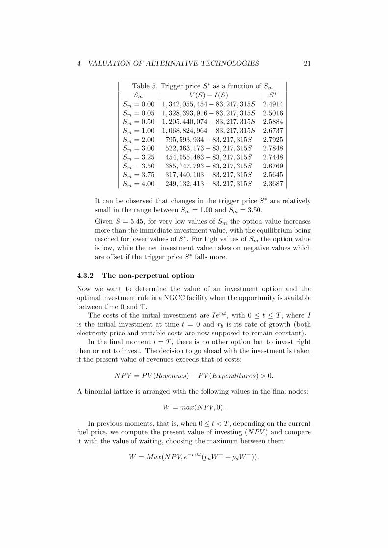
Table 5. Trigger price S∗ as a function of Sm

Sm V (S)− I(S) S∗

Sm = 0.00 1, 342, 055, 454− 83, 217, 315S 2.4914Sm = 0.05 1, 328, 393, 916− 83, 217, 315S 2.5016Sm = 0.50 1, 205, 440, 074− 83, 217, 315S 2.5884Sm = 1.00 1, 068, 824, 964− 83, 217, 315S 2.6737Sm = 2.00 795, 593, 934− 83, 217, 315S 2.7925Sm = 3.00 522, 363, 173− 83, 217, 315S 2.7848Sm = 3.25 454, 055, 483− 83, 217, 315S 2.7448Sm = 3.50 385, 747, 793− 83, 217, 315S 2.6769Sm = 3.75 317, 440, 103− 83, 217, 315S 2.5645Sm = 4.00 249, 132, 413− 83, 217, 315S 2.3687

It can be observed that changes in the trigger price S∗ are relativelysmall in the range between Sm = 1.00 and Sm = 3.50.

Given S = 5.45, for very low values of Sm the option value increasesmore than the immediate investment value, with the equilibrium beingreached for lower values of S∗. For high values of Sm the option valueis low, while the net investment value takes on negative values whichare offset if the trigger price S∗ falls more.

4.3.2 The non-perpetual option

Now we want to determine the value of an investment option and theoptimal investment rule in a NGCC facility when the opportunity is availablebetween time 0 and T.

The costs of the initial investment are Ierbt, with 0 ≤ t ≤ T , where Iis the initial investment at time t = 0 and rb is its rate of growth (bothelectricity price and variable costs are now supposed to remain constant).

In the final moment t = T , there is no other option but to invest rightthen or not to invest. The decision to go ahead with the investment is takenif the present value of revenues exceeds that of costs:

NPV = PV (Revenues)− PV (Expenditures) > 0.

A binomial lattice is arranged with the following values in the final nodes:

W = max(NPV, 0).

In previous moments, that is, when 0 ≤ t < T , depending on the currentfuel price, we compute the present value of investing (NPV ) and compareit with the value of waiting, choosing the maximum between them:

W = Max(NPV, e−r∆t(puW+ + pdW−)).


The lattice is solved backwards, which provides the time-0 value. Ifwe compare this value with that of an investment made at the outset, thedifference will be the value of the option to wait. Logically, this option’svalue will always be nonnegative.

By changing the initial value of the fuel unit cost it is possible todetermine the fuel price at which the option value switches from positive tozero. This will be the optimal exercise price at t = 0. Similarly, arranginga binomial lattice for the investment opportunity with maturity t < T andchanging the fuel price, the optimal exercise price for intermediate momentsis determined.

At the final date, investment is realized only if NPV > 0. The optimalpoint to invest will be found by computing the gas price for which NPV = 0;in our case, this value is S∗0 = 5.4563. As could be expected, when ra =rb = 0, it must be S∗∞ = 2.7448, which comes from the analytical solutionfor the perpetual option. These results appear in Table 6. They show aconvergence towards those of the perpetual option when the maturity of theinvestment opportunity increases.

Table 6. Trigger price S∗ with finite timeTerm ra = 0, rb = 0 ra = 0, rb = 0.025 ra = 0, rb = 0.05

0 5.4563 5.4563 5.456312 3.3268 3.5587 3.78231 3.2200 3.4417 3.65032 3.0864 3.3035 3.51073 3.0040 3.2250 3.43944 2.9480 3.1751 3.39825 2.9079 3.1413 3.37316 2.8782 3.1179 3.35757 2.8557 3.1012 3.34818 2.8386 3.0893 3.34239 2.8253 3.0808 3.339210 2.8151 3.0746 3.3378∞ 2.7448 - -

It can be observed that a higher rb, ceteris paribus, quickens the time toinvest, as can be seen from the higher S∗. When the time to maturity iszero, though, there is no influence from the rate of growth of the initialinvestment.

Next we analyze the optimal choice between investing or waiting, whenthe investment opportunity is available for five years, depending on theinitial fuel price.


Table 7. NPV and option values with T = 5 yearsS0 NPV(AC) Option value Max(NPV,Option) Optimal decision

5.45 521,120 119,170,000 119,170,000 Wait5.00 37,969,000 129,040,000 129,040,000 Wait4.50 79,578,000 141,640,000 141,640,000 Wait4.00 121,190,000 156,820,000 156,820,000 Wait3.50 162,790,000 176,420,000 176,420,000 Wait3.00 204,400,000 205,010,000 205,010,000 Wait

2.9079 212,070,000 212,070,000 212,070,000 Indifferent2.50 246,010,000 245,900,000 246,010,000 Invest2.00 287,620,000 287,450,000 287,620,000 Invest

As shown in Table 7, when S0 = 5.45, the NPV is very low and the option towait is worth more than 119 million euros. As the value of S0 decreases, theoption to wait increases in value but less than the NPV, with the equalitybeing reached when S0 = 2.9079. For lower values, it is preferable to investimmediately.

4.4 Valuation of an operating IGCC plant

Now we must compute the value of an operating IGCC power station, bothright upon the initial outlay and at any moment along its useful life to deriveits remaining value. We accomplish this by means of two two-dimensionalbinomial lattices which refer to initial states consuming either coal or naturalgas, respectively.

At the end of the plant’s useful life, its value is zero, whether that instanthas been reached consuming coal or natural gas:

Wc = 0 if useful life is finished consuming coal,Wg = 0 if useful life is finished consuming natural gas,

where Wc stands for the values of the lattice nodes for coal and Wg denotesthose of the lattice nodes for natural gas. At earlier times t we compute, fora time interval ∆t, the profits by mode of operation, which are determinedas the difference between electricity revenues and the sum of variable plusfuel costs:

πc = A.E.erat (1− e−∆t(r−ra))r − ra

−Bc∆tSc −A.Cvarc .erat (1− e−∆t(r−ra))

r − ra,

(56)

πg = A.E.erat (1− e−∆t(r−ra))r − ra

−Bg∆tSg −A.Cvarg .erat (1− e−∆t(r−ra))

r − ra.

(57)where:


πc : Net profits from operating with coal.πg : Net profits from operating with natural gas.Sc: current coal price,Sg: current natural gas price.

A.E.erat (1−e−∆t(r−ra))r−ra

: value at time t of revenues from electricity overthe period ∆t.

A.Cvar.erat (1−e−∆t(r−ra))

r−ra: value at time t of variable costs incurred over

∆t.Bc: the coal energy needed per year in GJ,Bg: the natural gas energy needed per year in GJ,Bc∆tSc : Costs of coal consumed during ∆t.Bg∆tSg : Costs of natural gas consumed during ∆t.I(c → g) : Switching cost from coal to gas.I(g → c) : Switching cost from gas to coal.If initially the IGCC plant was consuming coal, the best of two options

is chosen:20

• continue: the present value of the coal lattice is obtained, plus theprofits from operating in coal-mode at that instant.

• switch: the present value of the gas lattice is obtained, plus theprofits from operating in gas-mode at that instant, minus the coststo switching from coal to gas, I(c → g).

Thus the binomial lattices will take on the following values:21

Wc = Max(πc+e−r∆t(puuWc+++pudWc+−pduWc−++pddWc−−), πg−I(c → g)+

+e−r∆t(puuWg++ + pudWg+−pduWg−+ + pddWg−−)). (58)

Similary, when the initial state corresponds to operating with natural gas,we would compute:

Wg = Max(πc−I(g → c)+e−r∆t(puuWc+++pudWc+−pduWc−++pddWc−−),

πg + e−r∆t(puuWg++ + pudWg+−pduWg−+ + pddWg−−)). (59)

Finally, at time zero the optimal initial mode of operation is chosen by:

Max(Wc, Wg).20We have not considered the option not to operate, though it could be taken into

account easily. It could be included by a third lattice, corresponding to an idle initialstate. At every time we should maximize over three possible values, taking into accountthe switching costs between states. If we denote the idle state by p, in this case there couldbe a stopping cost: I(c→ p) or I(g → p), and a restarting cost: I(p→ c) or I(p→ g). Ifrestarting costs were very high, stopping could amount to abandone.

21We follow a similar procedure to Trigeorgis [20], pp. 177-184 (the case with switchingcosts).


In this way, we have derived the value of a flexible plant in operation.In this computation, for a plant operating for some time, the cost of the

initial investment plays no role, but it could be included at the outset inorder to compare this outlay with the present value of expected profits.

Table 8 shows the values adopted in the base case. Some of them aretaken from Table 1 but are repeated here for convenience.

Table 8. An IGCC PlantConcepts Coal Mode Gas Mode

Plant Size Mw (P) 500 500Production Factor(FP) 80% 80%

Net Efficiency(%) (RDTO) 41.0% 50.5%Investment cost AC/Kw (i) 1,300 1,300

Operation cost (ACcents/Kwh) (CVAR) 0.71 0.32Fuel price (AC/GJ) 1.90 5.45

Reversion value Sm(AC/GJ) 1.40 3.25Reversion speed (k) 0.125 0.25

Plant’s useful life (years)(τ) 25 25Risk-free interest rate (r) 0.05 0.05Market price of risk (φ) 0.40 0.40

Volatility (σ) 0.05 0.20Correlation with the market (ρ1, ρ2) 0 0

Correlation between fuels (ρ12) 0.15 0.15Investment cost rate of growth (rb) 0 0Electricity price rate of growth (ra) 0 0

Switching costs (AC) 20,000 20,000

Making the computations with a lattice of 300 steps (one for each monthof useful life), Table 9 shows the ensuing results, as a function of switchingcosts.

Table 9. Value of an IGCC PlantSwitching costs (AC) Plant’s value Plant’s value - Initial investment

0 702,662,000 52,662,00010,000 702,598,000 52,598,00020,000 702,534,000 52,534,00050,000 702,345,000 52,345,000100,000 702,129,000 52,129,000

1,000,000 700,049,000 50,049,000∞ 691,987,000 41,987,000

When there are no switching costs, the value of the plant exceeds the initialinvestment (650,000,000 AC) by 52,662,000 AC. Thus it is worth an 8.10%more than the amount disbursed.

Comparing the value in each case with that of infinite switching costs,the difference shows the value of flexibility, which amounts to 10,675,000


AC in the absence of switching costs, just 1.5% over the initial investment.Note tha flexibility in the IGCC plant may be valuable because of reasonsdifferent from harnessing at each instant the best fuel option. For instance,it may be due to failures in elements necessary to operate in coal-mode,but that do not prevent the plant from operating in gas-mode and avert thetotal stopping of the facility. The same could happen in the case of problemsconcerning supplies of a certain kind of fuel.

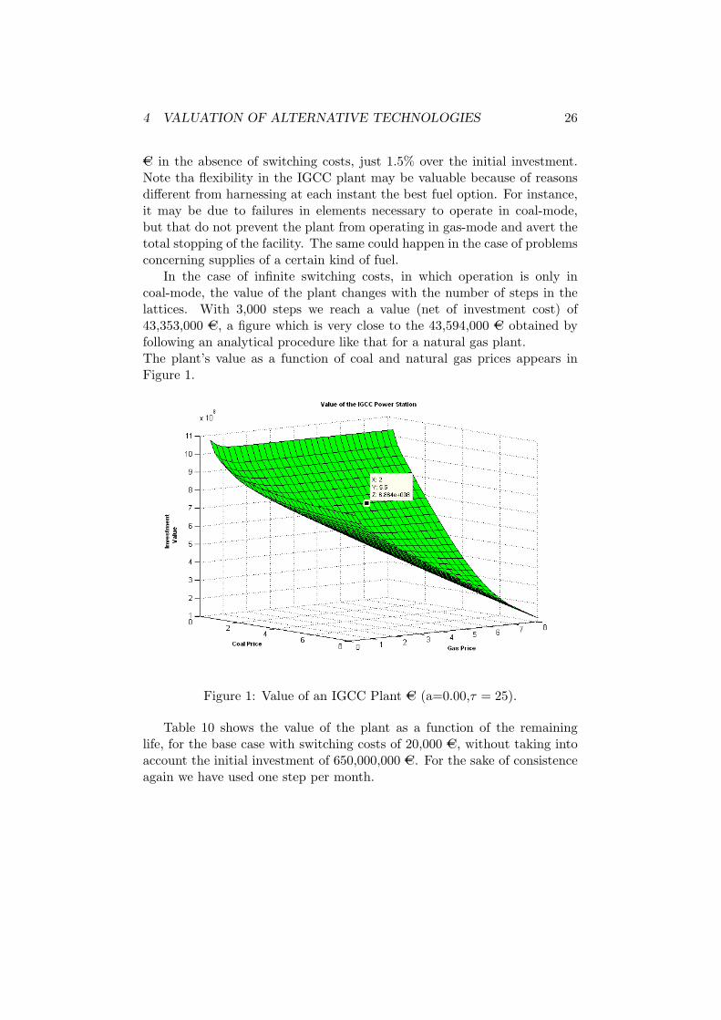
In the case of infinite switching costs, in which operation is only incoal-mode, the value of the plant changes with the number of steps in thelattices. With 3,000 steps we reach a value (net of investment cost) of43,353,000 AC, a figure which is very close to the 43,594,000 AC obtained byfollowing an analytical procedure like that for a natural gas plant.The plant’s value as a function of coal and natural gas prices appears inFigure 1.

Figure 1: Value of an IGCC Plant AC (a=0.00,τ = 25).

Table 10 shows the value of the plant as a function of the remaininglife, for the base case with switching costs of 20,000 AC, without taking intoaccount the initial investment of 650,000,000 AC. For the sake of consistenceagain we have used one step per month.


Table 10. Value of an operating IGCC plant as a function of thegrowth rate of electricity price and variable cost (ra)

Remaining life Plant value ra = 0.00 Plant value ra = 0.0325 years 702,534,000 1,245,700,00020 years 613,835,000 999,120,00015 years 501,490,000 742,186,00010 years 361,090,000 479,990,0005 years 191,020,000 223,980,0004 years 153,950,000 175,460,0003 years 116,150,000 128,500,0002 years 77,806,000 83,409,0001 year 39,044,000 40,477,0000 year 0 0

The shape of the curve for ra = 0 has to do with the discount rater = 0.05, since the electricity price remains unchanged. If ra = 0.03, thevalue with two years to operate exceeds twice that with one year since,because of the reversion effect, a bigger drop in fuel cost would be expectedover two remaining years.

4.5 Valuation of the opportunity to invest in an IGCC plant

Let us assume that the investment opportunity is available from time 0 toT . In this case, the procedure is very similar to that for the optimal timingto invest in a NGCC plant. However, the value of an operating plant mustbe determined at each node of the two-dimensional lattice from anothertwo-dimensional lattice which takes as a starting point the prices at thatnode.

At the final date, the choice must be made between investing then if theplant’s value is positive or not to invest:

W = max(NPVigcc, 0).

With switching costs of 20,000 AC as in the base case, Table 11 showscombinations of coal and natural gas prices that imply a zero value (that is,the plant value matches initial outlay) at maturity.


Table 11. IGCC Critical curve at t = T

Gas price (AC/GJ) Coal price (AC/GJ)∞ 2.1410

5.4563 2.23255.45 2.23275.00 2.24464.50 2.26424.00 2.29743.50 2.36843.25 2.44853.00 2.58022.50 3.06822.00 4.06101.50 6.26461.00 18.9226

0.9897 ∞

If, with a very high price for coal, the IGCC plant is to be profitable, itis necessary that natural gas prices remain below 0.9897. This is due to thefact that the reversion process pushes gas prices towards 3.25 AC/GJ.

At previous instants, the best of the two options (to invest or to continue)has to be chosen:

W = Max(NPVigcc, e−r∆t(puuW++ + pudW

+−pduW−+ + pddW−−)). (60)

At t = 0, the value obtained from the lattice is compared with that of aninvestment realized right then. The difference is the value of the option towait.

By using a lattice with quarterly steps for the option to wait, and onewith monthly steps to value the plant, we get the valuations in Table 12,for the base case, as a function of the time to maturity of the investmentoption:

Table 12. Value of the option to wait (IGCC plant)Term (years) Plant NPV Option to wait Option to wait - Plant NPV

5 52,534,000 76,398,000 23,864,0004 52,534,000 74,179,000 21,645,0003 52,534,000 71,048,000 18,514,0002 52,534,000 66,651,000 14,117,0001 52,534,000 60,592,000 8,058,000

0.5 52,534,000 56,835,000 4,301,0000 52,534,000 52,534,000 0

The second column refers to the plant value under the assumption of a “nowor never” investment in the flexible technology. It includes the value of theplant’s flexibility.


The value of the option to wait, given the starting point of the prices,increases with the maturity of the opportunity to invest. The highest yearlyincrease takes place in the first period (8, 058, 000 AC); henceforth, thatincrease is much lower, since the effect of reversion is stronger in the initialperiods.22

The optimal investment rule in an IGCC technology can be derived followinga procedure akin to that used for the NGCC technology in the base case.Nonetheless, in this case and at each time, we will have to compute thecombinations of coal price and gas price for which the option to wait isworthless.

At any t, a range of initial prices for coal is chosen; then, for each one ofthem, we compute the natural gas price for which the option to wait turnsfrom positive to zero. For an option to wait up to two years, we get Table13.

Table 13. Optimal values with option to wait 2 years (IGCC)Gas price Coal price

∞ 1.575.45 1.565.00 1.564.50 1.564.00 1.563.50 1.563.25 1.573.00 1.572.50 1.592.25 1.852.00 2.981.50 5.150.96 ∞

These results are shown in Figure 2. It can be observed that the curve hasshifted downwards and to the left, in relation to the case in which there is nooption to wait (Table 11). In other words, it makes sense to give up (“kill”)the option to wait if the prices are relatively lower but not otherwise.For a natural gas price of 5.00AC/GJ, the resulting values for the investmentin the IGCC plant and for the option to wait appear in Figure 3. As canbe observed, given a natural gas price of 5.00AC/GJ, it is better to invest ifcoal price is low, but one must wait if coal price is high.

22With t1/2 = ln(2)k

one would guess that gas price will change from 5.45 AC/GJ to4.35 AC/GJ in 2.77 years time. On the other hand, the expected price for coal 5.55 yearsfrom now would be 1.65 AC/GJ. The value of t1/2 results from solving: S0 − (S0−Sm

2) =

Sm + (S0 − Sm)e−kt1/2 .


Figure 2: Border of Continuation area for investment in an IGCC PowerPlant with option to wait for two years.

4.6 Valuation of the opportunity to invest in NGCC orIGCC

Up to now we have considered both the flexible and the inflexibletechnologies in isolation. When there is an opportunity to invest in eitherone of the two technologies, at each moment we face the choice:

• to invest in the inflexible technology (NGCC),

• to invest in the flexible technology (IGCC),

• to wait and at maturity give up the investment.

At the final date, since there is no remaining option, the best alternativeamong the three available is chosen:

W = max(NPVigcc, NPVngcc, 0),

where the value NPVigcc, at each point in the binomial lattice, iscomputed by means of a two-dimensional binomial lattice with the fuel pricesat that node.

If, at time T , the only possibility is to invest in the NGCC technology,the investment is realized whenever the natural gas price is lower than 5.4563


Figure 3: Values of the investment and the option to wait for two years.

AC/GJ; see Table 6. Similarly, if, at time T , the only alternative is to invest inthe IGCC technology, the plant is built when the combinations of gas priceand coal price lay below the curve resulting from Table 11. Now Figure 4shows both decision rules, but it must be remembered that, in this case, itis not possible to choose the best possibility.

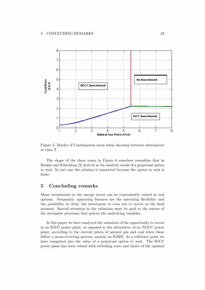
When, at time T , it is possible to choose between the two alternatives(Figure 5), there is a set of combinations natural gas price-coal price suchthat the value of the investment is positive for the two plants; consequentlythe investment with the highest value will be chosen. This area will bedivided into two by a line starting at the point (Sg = 5.4563;Sc = 2.2325),along which there is indifference among investing in IGCC, investing inNGCC, and not investing. There is also a region in which the optimaldecision is not to invest.

At previous moments, the choice is:

W = max(NPVigcc, NPVngcc, e−r∆t(puuW+++pudW

+−pduW−++pddW−−)).

This computing procedure is iteratively followed until the initial value isobtained. At that instant, the NGCC technology will be adopted if W =NPVngcc; similarly, the IGCC technology is chosen if W = NPVigcc. If thereis no investment at t = 0, this means that the best option is to wait.

The points along the optimal exercise curve are those for which the valueof the option to wait changes from positive to zero. In principle, there maybe two curves, one for the IGCC plant and another one for the NGCC plant.See Figure 6 for an option to invest with two years to maturity. It can be


Figure 4: Border of Continuation areas without choosing betweenalternatives at time T.

observed that:

• In order to invest, prices must be rather lower than those when thereis no option to wait. The reversion effect, given the initial prices,promotes this behaviour.

• For a very high natural gas price, there will be investment in an IGCCplant if coal price is below 1.57 AC/GJ, which is the same that wecomputed for the waiting option in the IGCC investment and this wasthe only technology available (Table 13).

• Similarly, for a very high coal price, there will be investment in aGNCC plant if gas price is below 3.17 AC/GJ.23

• For values close to the iso-value line between immediate investmentin NGCC and IGCC, the best choice is to wait in order to see howuncertainty unfolds. The waiting zone expands into the regions ofimmediate investment like a wedge.

23This result would apply as an option to wait for two years in a NGCC plant with alattice of 8 steps, the same step size used in the option to wait with the two technologieson offer.

5 CONCLUDING REMARKS 33

Figure 5: Border of Continuation areas when choosing between alternativesat time T.

The shape of the three zones in Figure 6 somehow resembles that inBrekke and Schieldrop [3] derived as the analytic result of a perpetual optionto wait. In our case the solution is numerical because the option to wait isfinite.

5 Concluding remarks

Many investments in the energy sector can be conveniently valued as realoptions. Frequently appearing features are the operating flexibility andthe possibility to delay the investment or even not to invest at the finalmoment. Special attention in the valuation must be paid to the nature ofthe stochastic processes that govern the underlying variables.

In this paper we have analyzed the valuation of the opportunity to investin an IGCC power plant, as opposed to the alternative of an NGCC powerplant, according to the current prices of natural gas and coal when thesefollow a mean-reverting process, namely an IGBM. As a reference point wehave computed also the value of a perpetual option to wait. The IGCCpower plant has been valued with switching costs and choice of the optimal

5 CONCLUDING REMARKS 34

Figure 6: Border of Continuation areas when selecting between alternativeswith option to wait for two years.

mode of operation; actual parameters from an operating plant have beenused.First we have computed the value of an operating NGCC plant. This isrelatively easy since there is no special flexibility in its usage. Then thevalue of a perpetual option to invest in it has been estimated; besides, asensitivity analysis has been developed. It has served as a limiting case orreference point for the finite-lived option. This has been valued by meansof a binomial lattice for different maturities and growth rates of electricityprice and investment outlay. The optimal investment rule for a given termas a function of natural gas price has also been analyzed.Second we have valued an IGCC plant in operation using twotwo-dimensional lattices, depending on whether initially the plant is coal- ornatural gas-fired. The value of the plant has been computed as a function ofswitching costs and for different useful life spans with constant or growingelectricity prices. Next the non-perpetual option to invest in an IGCCplant has been considered, assuming again that this is the only technologyavailable. In this case, an optimal locus of fuel prices arises above which itis optimal to wait. As could be expected, the longer the option’s maturitythe closer the locus is to the origin in the prices space.

A VALUATION OF AN ANNUITY IN PRESENCE OF MEAN REVERSION35

Third we have assumed that both technologies are on offer. Our resultsshow the influence of the mean-reverting process on the critical values whencurrent fuel prices are above their level expected in the long run. The valueof the operating flexibility in the IGCC power plant seems to be low, becauseit is designed to function mainly with coal. We show that prior to option‘smaturity there is a small region in the prices space in which it is optimalto wait instead of investing, since the values of both technologies are veryclose; outside it, optimal decisions are clear-cut.

A Valuation of an annuity in presence of meanreversion

Our aim is to value an asset V wich pays Xdt continuously over afinite number of periods τ of remaining asset life, with X following amean-reverting process of the type:

dX = k(Xm −X)dt + σXdZt.

It can be shown that the asset V satisfies the differential equation:

12VXXσ2X2 + (k(Xm −X)− ρσφX)VX − rV − Vτ = −X, (61)

where it is assumed that the existing traded assets dynamically span theprice X. Let ρ denote the correlation with the market portfolio, and φ themarket price of risk:

φ =(rM − r)

σM,

where rM stands for the expected return on the market portfolio and σM itsstandard deviation. The solution V (X, τ) to the differential equation mustsatisfy the following boundary conditions:

• At τ = 0 the value must be zero: V (X, 0) = 0,

• Bounded derivative as X →∞: VX(∞, τ) < ∞,

• Bounded derivative as X → 0: VX(0, τ) < ∞.

Using Laplace transforms we get:

12hXXσ2X2 + (k(Xm −X)− ρσφX)hX − h(r + s) = −X

s.

Rearranging:

12hXXσ2X2 − (k + ρσφ)XhX − h(r + s) = −kXmhX −

X

s.

A VALUATION OF AN ANNUITY IN PRESENCE OF MEAN REVERSION36

The general solution has the form:

h(X) = A1Xβ1 + A2X

β2 +X − kXm

k+ρσφ

s(s + r + k + ρσφ)+

kXm

(k + ρσφ)s(s + r).

The derivative is bounded; thus A1 = 0. Besides, h(0) = 0; therefore A2 = 0.The solution simplifies to:

h(X) =X − kXm

k+ρσφ

s(s + r + k + ρσφ)+

kXm

(k + ρσφ)s(s + r).

With the first and second derivatives: hX = 1s(s+r+k+ρσφ) , hXX = 0, it is

possible to show, by substitution, that the differential equation applies.At this moment, the inverse Laplace transforms are taken. To do so we

use formula 29.3.12 in Abramowitz and Stegun [1], the final result being:

V =kXm(1− e−rτ)

r(k + ρσφ)+

X − kXmk+ρσφ

r + k + ρσφ(1− e−(r+k+ρσφ)τ ). (62)

This formula may be useful to compute the present value of fuel costs overthe whole life of a plant with inflexible technology, like an NGCC or coalplant.24

A series of particular, frequently used, cases may be derived from theabove general solution:

• a) If φ = 0 or ρ = 0, then the formula reduces to

V =Xm(1− e−rτ )

r+

X −Xm

r + k(1− e−(r+k)τ ).

• b) If τ →∞:

V =kXm

r(k + ρσφ)+

X − kXmk+ρσφ

r + k + ρσφ. (63)

In this case, it can be observed that the project value is the sum oftwo components: one related to the reversion value and another onewhich is a function of the initial difference between the observed valueand the ”normal” level of X.

• c) When it is a perpetuity and also Xm = 0 and k + ρσφ = −α, then:

V =X

r − α. (64)

• d) When it is a perpetuity and also Xm = 0 and k + ρσφ = −r + δ,then:

V =X

δ. (65)

24See Bhattacharya [2](eq. 15) and Sarkar [15] (eq. 2-4).

REFERENCES 37

References

[1] M. Abramowitz and I. Stegun. Handbook of Mathematical Functions.Dover Publications, 1972.

[2] S. Bhattacharya. Project valuation with mean-reverting cash flowstreams. Journal of Finance, XXXIII(5):1317-1331, 1978.

[3] J.A. Brekke and B. Schieldrop. Investment in Flexible Technologiesunder Uncertainty. In: Brennan M. J. and L. Trigeorgis (eds.), ProjectFlexibility, Agency and Competition, , Oxford University Press, 2000,34-49.

[4] M.J. Brennan and L. Trigeorgis. Project Flexibility, Agency, andCompetition. Oxford University Press, 2000.

[5] L. Clewlow and C. Strickland. Implementing Derivatives Models. JohnWiley and Sons, Inc., 1998.

[6] A. K. Dixit and R. S. Pindyck. Investment under Uncertainty.Princeton University Press, 1994.

[7] O. Herbelot. Option Valuation of Flexible Investments: The Case ofEnvironmental Investments in the Electric Power Industry. PhD thesis,Massachusetts Institute of Technology, 1992.

[8] M. Insley. A real option approach to the valuation of a forestryinvestment. Journal of Environmental Economics and Management,44:471-492, 2002.

[9] P. E. Kloeden and E. Platen. Numerical Solution of StochasticDifferential Equations. Springer, 1992.

[10] N. Kulatilaka. Valuing the flexibility of flexible manufacturing systems.IEEE Transactions on Engineering Management, 35(4):250-257, 1988.

[11] N. Kulatilaka. The value of flexibility: The case of a dual-fuel steamboiler. Financial Management, 22(3):271-279, 1993.

[12] N. Kulatilaka. The Value of Flexibility: A General Model ofReal Options. In: Lenos Trigeorgis (ed.), Real Options in CapitalInvestment. Praeger, 1995.

[13] J. Mun. Real Option Analysis. John Wiley and Sons, Inc., 2002.

[14] G. F. Robel. Real options and mean-reverting prices. The 5th AnnualReal Options Conference, 2001.

REFERENCES 38

[15] S. Sarkar. The effect of mean reversion on investment underuncertainty. Journal of Economic Dynamics and Control, 28:377-396,2003.

[16] E. S. Schwartz. The stochastic behavior of commodity prices:Implications for valuation and hedging. Journal of Finance,52(3):923-973, 1997.

[17] E. S. Schwartz and L. Trigeorgis. Real Options and Investment underUncertainty. MIT, 2001.

[18] D. C. Shimko. Finance in Continuous Time: A Primer. KolbPublishing Company, 1992.

[19] G. Sick. Real options. In: Jarrow R. et al. (eds) Handbooks inOperations Research and Management Science, vol 9, Elsevier Science1995, 631-691.

[20] L. Trigeorgis. Real Options - Managerial Flexibility and Strategyin Resource Allocation. The MIT Press, Cambridge, Massachusetts,1996.

valuing flexibility: the case of an integrated

Documents