Value Prediction Network

Junhyuk Oh† Satinder Singh† Honglak Lee∗,††University of Michigan

∗Google Brain{junhyuk,baveja,honglak}@umich.edu, honglak@google.com

AbstractThis paper proposes a novel deep reinforcement learning (RL) architecture, calledValue Prediction Network (VPN), which integrates model-free and model-basedRL methods into a single neural network. In contrast to typical model-basedRL methods, VPN learns a dynamics model whose abstract states are trainedto make option-conditional predictions of future values (discounted sum of re-wards) rather than of future observations. Our experimental results show thatVPN has several advantages over both model-free and model-based baselines in astochastic environment where careful planning is required but building an accurateobservation-prediction model is difficult. Furthermore, VPN outperforms DeepQ-Network (DQN) on several Atari games even with short-lookahead planning,demonstrating its potential as a new way of learning a good state representation.

1 Introduction

Model-based reinforcement learning (RL) approaches attempt to learn a model that predicts futureobservations conditioned on actions and can thus be used to simulate the real environment and domulti-step lookaheads for planning. We will call such models an observation-prediction model todistinguish it from another form of model introduced in this paper. Building an accurate observation-prediction model is often very challenging when the observation space is large [24, 6, 14, 4] (e.g., high-dimensional pixel-level image frames), and even more difficult when the environment is stochastic.Therefore, a natural question is whether it is possible to plan without predicting future observations.

In fact, raw observations may contain information unnecessary for planning, such as dynamicallychanging backgrounds in visual observations that are irrelevant to their value/utility. The starting pointof this work is the premise that what planning truly requires is the ability to predict the rewards andvalues of future states. An observation-prediction model relies on its predictions of observations topredict future rewards and values. What if we could predict future rewards and values directly withoutpredicting future observations? Such a model could be more easily learnable for complex domains ormore flexible for dealing with stochasticity. In this paper, we address the problem of learning andplanning from a value-prediction model that can directly generate/predict the value/reward of futurestates without generating future observations.

Our main contribution is a novel neural network architecture we call the Value Prediction Network(VPN). The VPN combines model-based RL (i.e., learning the dynamics of an abstract state spacesufficient for computing future rewards and values) and model-free RL (i.e., mapping the learnedabstract states to rewards and values) in a unified framework. In order to train a VPN, we proposea combination of temporal-difference search [29] (TD search) and n-step Q-learning [21]. In brief,VPNs learn to predict values via Q-learning and rewards via supervised learning. At the same time,VPNs perform lookahead planning to choose actions and compute bootstrapped target Q-values.

Our empirical results on a 2D navigation task demonstrate the advantage of VPN over model-freebaselines (e.g., Deep Q-Network [22]). We also show that VPN is more robust to stochasticity in theenvironment than an observation-prediction model approach. Furthermore, we show that our VPNoutperforms DQN on several Atari games [2] even with short-lookahead planning, which suggests

31st Conference on Neural Information Processing Systems (NIPS 2017), Long Beach, CA, USA.

arX

iv:1

707.

0349

7v2

[cs

.AI]

6 N

ov 2

017

that our approach can be potentially useful for learning better abstract-state representations andreducing sample-complexity.

2 Related Work

Model-based Reinforcement Learning. Dyna-Q [33, 35, 40] integrates model-free and model-based RL by learning an observation-prediction model and using it to generate samples for Q-learningin addition to the model-free samples obtained by acting in the real environment. Gu et al. [8]extended these ideas to continuous control problems. Our work is similar to Dyna-Q in the sense thatplanning and learning are integrated into one architecture. However, VPNs perform a lookahead treesearch to choose actions and compute bootstrapped targets, whereas Dyna-Q uses a learned modelto generate imaginary samples. In addition, Dyna-Q learns a model of the environment separatelyfrom a value function approximator. In contrast, the dynamics model in VPN is combined with thevalue function approximator in a single neural network and indirectly learned from reward and valuepredictions through backpropagation.

Another line of work [24, 4, 9, 31] uses observation-prediction models not for planning, but for improv-ing exploration. A key distinction from these prior works is that our method learns abstract-state dy-namics not to predict future observations, but instead to predict future rewards/values. For continuouscontrol problems, deep learning has been combined with model predictive control (MPC) [7, 19, 27],a specific way of using an observation-prediction model. In cases where the observation-predictionmodel is differentiable with respect to continuous actions, backpropagation can be used to find theoptimal action [20] or to compute value gradients [12]. In contrast, our work focuses on learning andplanning using lookahead for discrete control problems.

Our VPNs are related to Value Iteration Networks [36] (VINs) which perform value iteration (VI) byapproximating the Bellman-update through a convolutional neural network (CNN). However, VINsperform VI over the entire state space, which in practice requires that 1) the state space is small andrepresentable as a vector with each dimension corresponding to a separate state and 2) the states havea topology with local transition dynamics (e.g., 2D grid). VPNs do not have these limitations and arethus more generally applicable, as we will show empirically in this paper.

VPN is close to and in-part inspired by Predictron [30] in that a recurrent neural network (RNN) actsas a transition function over abstract states. VPN can be viewed as a grounded Predictron in that eachrollout corresponds to the transition in the environment, whereas each rollout in Predictron is purelyabstract. In addition, Predictrons are limited to uncontrolled settings and thus policy evaluation,whereas our VPNs can learn an optimal policy in controlled settings.

Model-free Deep Reinforcement Learning. Mnih et al. [22] proposed the Deep Q-Network(DQN) architecture which learns to estimate Q-values using deep neural networks. A lot of variationsof DQN have been proposed for learning better state representation [38, 17, 10, 23, 37, 25], includingthe use of memory-based networks for handling partial observability [10, 23, 25], estimating bothstate-values and advantage-values as a decomposition of Q-values [38], learning successor staterepresentations [17], and learning several auxiliary predictions in addition to the main RL values [13].Our VPN can be viewed as a model-free architecture which 1) decomposes Q-value into reward,discount, and the value of the next state and 2) uses multi-step reward/value predictions as auxiliarytasks to learn a good representation. A key difference from the prior work listed above is that ourVPN learns to simulate the future rewards/values which enables planning. Although STRAW [37]can maintain a sequence of future actions using an external memory, it cannot explicitly performplanning by simulating future rewards/values.

Monte-Carlo Planning. Monte-Carlo Tree Search (MCTS) methods [16, 3] have been used forcomplex search problems, such as the game of Go, where a simulator of the environment is alreadyavailable and thus does not have to be learned. Most recently, AlphaGo [28] introduced a valuenetwork that directly estimates the value of state in Go in order to better approximate the value ofleaf-node states during tree search. Our VPN takes a similar approach by predicting the value ofabstract future states during tree search using a value function approximator. Temporal-differencesearch [29] (TD search) combined TD-learning with MCTS by computing target values for a valuefunction approximator through MCTS. Our algorithm for training VPN can be viewed as an instanceof TD search, but it learns the dynamics of future rewards/values instead of being given a simulator.

2

(a) One-step rollout (b) Multi-step rolloutFigure 1: Value prediction network. (a) VPN learns to predict immediate reward, discount, and the value of thenext abstract-state. (b) VPN unrolls the core module in the abstract-state space to compute multi-step rollouts.

3 Value Prediction Network

The value prediction network is developed for semi-Markov decision processes (SMDPs). Let xt bethe observation or a history of observations for partially observable MDPs (henceforth referred toas just observation) and let ot be the option [34, 32, 26] at time t. Each option maps observationsto primitive actions, and the following Bellman equation holds for all policies π: Qπ(xt, ot) =

E[∑k−1i=0 γ

irt+i + γkV π(xt+k)], where γ is a discount factor, rt is the immediate reward at time t,and k is the number of time steps taken by the option ot before terminating in observation xt+k.

A VPN not only learns an option-value function Qθ (xt, ot) through a neural network parameterizedby θ like model-free RL, but also learns the dynamics of the rewards/values to perform planning. Wedescribe the architecture of VPN in Section 3.1. In Section 3.2, we describe how to perform planningusing VPN. Section 3.3 describes how to train VPN in a Q-Learning-like framework [39].

3.1 Architecture

The VPN consists of the following modules parameterized by θ = {θenc, θvalue, θout, θtrans}:

Encoding fencθ : x 7→ s Value fvalueθ : s 7→ Vθ(s)Outcome foutθ : s, o 7→ r, γ Transition f transθ : s, o 7→ s′

• Encoding module maps the observation (x) to the abstract state (s ∈ Rm) using neural networks(e.g., CNN for visual observations). Thus, s is an abstract-state representation which will belearned by the network (and not an environment state or even an approximation to one).

• Value module estimates the value of the abstract-state (Vθ(s)). Note that the value module is not afunction of the observation, but a function of the abstract-state.

• Outcome module predicts the option-reward (r ∈ R) for executing the option o at abstract-states. If the option takes k primitive actions before termination, the outcome module should predictthe discounted sum of the k immediate rewards as a scalar. The outcome module also predicts theoption-discount (γ ∈ R) induced by the number of steps taken by the option.

• Transition module transforms the abstract-state to the next abstract-state (s′ ∈ Rm) in an option-conditional manner.

Figure 1a illustrates the core module which performs 1-step rollout by composing the above modules:f coreθ : s, o 7→ r, γ, Vθ(s′), s′. The core module takes an abstract-state and option as input and makesseparate option-conditional predictions of the option-reward (henceforth, reward), the option-discount(henceforth, discount), and the value of the abstract-state at option-termination. By combining thepredictions, we can estimate the Q-value as follows: Qθ(s, o) = r + γVθ(s′). In addition, the VPNrecursively applies the core module to predict the sequence of future abstract-states as well as rewardsand discounts given an initial abstract-state and a sequence of options as illustrated in Figure 1b.

3.2 Planning

VPN has the ability to simulate the future and plan based on the simulated future abstract-states.Although many existing planning methods (e.g., MCTS) can be applied to the VPN, we implementa simple planning method which performs rollouts using the VPN up to a certain depth (say d),henceforth denoted as planning depth, and aggregates all intermediate value estimates as described inAlgorithm 1 and Figure 2. More formally, given an abstract-state s = fencθ (x) and an option o, the

3

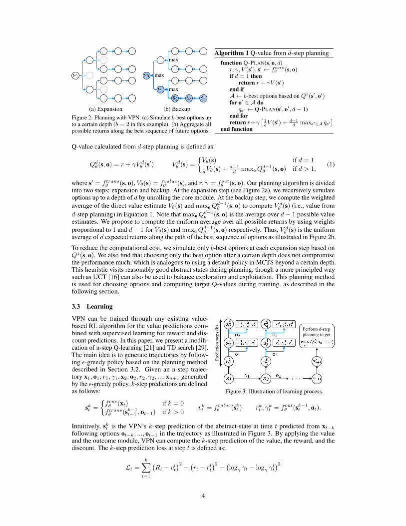
(a) Expansion (b) BackupFigure 2: Planning with VPN. (a) Simulate b-best options upto a certain depth (b = 2 in this example). (b) Aggregate allpossible returns along the best sequence of future options.

Algorithm 1 Q-value from d-step planningfunction Q-PLAN(s, o, d)

r, γ, V (s′), s′ ← fcoreθ (s, o)if d = 1 then

return r + γV (s′)end ifA ← b-best options based on Q1(s′, o′)for o′ ∈ A do

qo′ ← Q-PLAN(s′, o′, d− 1)end forreturn r+γ

[1dV (s′) + d−1

dmaxo′∈A qo′

]end function

Q-value calculated from d-step planning is defined as:

Qdθ(s, o) = r + γV dθ (s′) V dθ (s) =

{Vθ(s) if d = 11dVθ(s) +

d−1d maxo Q

d−1θ (s, o) if d > 1,

(1)

where s′ = f transθ (s, o), Vθ(s) = fvalueθ (s), and r, γ = foutθ (s, o). Our planning algorithm is dividedinto two steps: expansion and backup. At the expansion step (see Figure 2a), we recursively simulateoptions up to a depth of d by unrolling the core module. At the backup step, we compute the weightedaverage of the direct value estimate Vθ(s) and maxo Q

d−1θ (s, o) to compute V dθ (s) (i.e., value from

d-step planning) in Equation 1. Note that maxo Qd−1θ (s, o) is the average over d− 1 possible value

estimates. We propose to compute the uniform average over all possible returns by using weightsproportional to 1 and d− 1 for Vθ(s) and maxo Q

d−1θ (s, o) respectively. Thus, V dθ (s) is the uniform

average of d expected returns along the path of the best sequence of options as illustrated in Figure 2b.

To reduce the computational cost, we simulate only b-best options at each expansion step based onQ1(s, o). We also find that choosing only the best option after a certain depth does not compromisethe performance much, which is analogous to using a default policy in MCTS beyond a certain depth.This heuristic visits reasonably good abstract states during planning, though a more principled waysuch as UCT [16] can also be used to balance exploration and exploitation. This planning methodis used for choosing options and computing target Q-values during training, as described in thefollowing section.

3.3 Learning

Figure 3: Illustration of learning process.

VPN can be trained through any existing value-based RL algorithm for the value predictions com-bined with supervised learning for reward and dis-count predictions. In this paper, we present a modifi-cation of n-step Q-learning [21] and TD search [29].The main idea is to generate trajectories by follow-ing ε-greedy policy based on the planning methoddescribed in Section 3.2. Given an n-step trajec-tory x1, o1, r1, γ1, x2, o2, r2, γ2, ..., xn+1 generatedby the ε-greedy policy, k-step predictions are definedas follows:

skt =

{fencθ (xt) if k = 0

f transθ (sk−1t−1 , ot−1) if k > 0vkt = fvalueθ (skt ) rkt , γ

kt = foutθ (sk−1t , ot).

Intuitively, skt is the VPN’s k-step prediction of the abstract-state at time t predicted from xt−kfollowing options ot−k, ..., ot−1 in the trajectory as illustrated in Figure 3. By applying the valueand the outcome module, VPN can compute the k-step prediction of the value, the reward, and thediscount. The k-step prediction loss at step t is defined as:

Lt =k∑l=1

(Rt − vlt

)2+(rt − rlt

)2+(logγ γt − logγ γ

lt

)2

4

where Rt =

{rt + γtRt+1 if t ≤ nmaxo Q

dθ−(sn+1, o) if t = n+ 1

is the target value, and Qdθ−(sn+1, o) is the Q-

value computed by the d-step planning method described in 3.2. Intuitively, Lt accumulates lossesover 1-step to k-step predictions of values, rewards, and discounts. We find that applying logγ forthe discount prediction loss helps optimization, which amounts to computing the squared loss withrespect to the number of steps.

Our learning algorithm introduces two hyperparameters: the number of prediction steps (k) andplanning depth (dtrain) used for choosing options and computing bootstrapped targets. We also makeuse of a target network parameterized by θ− which is synchronized with θ after a certain numberof steps to stabilize training as suggested by [21]. The loss is accumulated over n-steps and theparameter is updated by computing its gradient as follows: ∇θL =

∑nt=1∇θLt. The full algorithm

is described in the Appendix.

3.4 Relationship to Existing Approaches

VPN is model-based in the sense that it learns an abstract-state transition function sufficient to predictrewards/discount/values. Meanwhile, VPN can also be viewed as model-free in the sense that itlearns to directly estimate the value of the abstract-state. From this perspective, VPN exploits severalauxiliary prediction tasks, such as reward and discount predictions to learn a good abstract-staterepresentation. An interesting property of VPN is that its planning ability is used to compute thebootstrapped target as well as choose options during Q-learning. Therefore, as VPN improves thequality of its future predictions, it can not only perform better during evaluation through its improvedplanning ability, but also generate more accurate target Q-values during training, which encouragesfaster convergence compared to conventional Q-learning.

4 Experiments

Our experiments investigated the following questions: 1) Does VPN outperform model-free baselines(e.g., DQN)? 2) What is the advantage of planning with a VPN over observation-based planning? 3)Is VPN useful for complex domains with high-dimensional sensory inputs, such as Atari games?

4.1 Experimental Setting

Network Architecture. A CNN was used as the encoding module of VPN, and the transitionmodule consists of one option-conditional convolution layer which uses different weights dependingon the option followed by a few more convolution layers. We used a residual connection [11] fromthe previous abstract-state to the next abstract-state so that the transition module learns the changeof the abstract-state. The outcome module is similar to the transition module except that it does nothave a residual connection and two fully-connected layers are used to produce reward and discount.The value module consists of two fully-connected layers. The number of layers and hidden units varydepending on the domain. These details are described in the Appendix.

Implementation Details. Our algorithm is based on asynchronous n-step Q-learning [21] wheren is 10 and 16 threads are used. The target network is synchronized after every 10K steps.We used the Adam optimizer [15], and the best learning rate and its decay were chosen from{0.0001, 0.0002, 0.0005, 0.001} and {0.98, 0.95, 0.9, 0.8} respectively. The learning rate is multi-plied by the decay every 1M steps. Our implementation is based on TensorFlow [1].1

VPN has four more hyperparameters: 1) the number of predictions steps (k) during training, 2) theplan depth (dtrain) during training, 3) the plan depth (dtest) during evaluation, and 4) the branchingfactor (b) which indicates the number of options to be simulated for each expansion step duringplanning. We used k = dtrain = dtest throughout the experiment unless otherwise stated. VPN(d)represents our model which learns to predict and simulate up to d-step futures during training andevaluation. The branching factor (b) was set to 4 until depth of 3 and set to 1 after depth of 3, whichmeans that VPN simulates 4-best options up to depth of 3 and only the best option after that.

Baselines. We compared our approach to the following baselines.

1The code is available on https://github.com/junhyukoh/value-prediction-network.

5

(a) Observation (b) DQN’s trajectory (c) VPN’s trajectoryFigure 4: Collect domain. (a) The agent should collect as manygoals as possible within a time limit which is given as additionalinput. (b-c) DQN collects 5 goals given 20 steps, while VPN(5)found the optimal trajectory via planning which collects 6 goals.

(a) Plan with 20 steps (b) Plan with 12 stepsFigure 5: Example of VPN’s plan. VPNcan plan the best future options just fromthe current state. The figures show VPN’sdifferent plans depending on the time limit.

• DQN: This baseline directly estimates Q-values as its output and is trained through asynchronousn-step Q-learning. Unlike the original DQN, however, our DQN baseline takes an option asadditional input and applies an option-conditional convolution layer to the top of the last encodingconvolution layer, which is very similar to our VPN architecture.2

• VPN(1): This is identical to our VPN with the same training procedure except that it performsonly 1-step rollout to estimate Q-value as shown in Figure 1a. This can be viewed as a variation ofDQN that predicts reward, discount, and the value of the next state as a decomposition of Q-value.

• OPN(d): We call this Observation Prediction Network (OPN), which is similar to VPN except thatit directly predicts future observations. More specifically, we train two independent networks: amodel network (fmodel : x, o 7→ r, γ, x′) which predicts reward, discount, and the next observation,and a value network (fvalue : x 7→ V (x)) which estimates the value from the observation. Thetraining scheme is similar to our algorithm except that a squared loss for observation prediction isused to train the model network. This baseline performs d-step planning like VPN(d).

4.2 Collect Domain

Task Description. We defined a simple but challenging 2D navigation task where the agent shouldcollect as many goals as possible within a time limit, as illustrated in Figure 4. In this task, theagent, goals, and walls are randomly placed for each episode. The agent has four options: moveleft/right/up/down to the first crossing branch or the end of the corridor in the chosen direction. Theagent is given 20 steps for each episode and receives a positive reward (2.0) when it collects a goal bymoving on top of it and a time-penalty (−0.2) for each step. Although it is easy to learn a sub-optimalpolicy which collects nearby goals, finding the optimal trajectory in each episode requires carefulplanning because the optimal solution cannot be computed in polynomial time.

An observation is represented as a 3D tensor (R3×10×10) with binary values indicating the pres-ence/absence of each object type. The time remaining is normalized to [0, 1] and is concatenated tothe 3rd convolution layer of the network as a channel.

We evaluated all architectures first in a deterministic environment and then investigated the robustnessin a stochastic environment separately. In the stochastic environment, each goal moves by one blockwith probability of 0.3 for each step. In addition, each option can be repeated multiple times withprobability of 0.3. This makes it difficult to predict and plan the future precisely.

Overall Performance. The result is summarized in Figure 6. To understand the quality of differentpolicies, we implemented a greedy algorithm which always collects the nearest goal first and ashortest-path algorithm which finds the optimal solution through exhaustive search assuming thatthe environment is deterministic. Note that even a small gap in terms of reward can be qualitativelysubstantial as indicated by the small gap between greedy and shortest-path algorithms.

The results show that many architectures learned a better-than-greedy policy in the deterministic andstochastic environments except that OPN baselines perform poorly in the stochastic environment. Inaddition, the performance of VPN is improved as the plan depth increases, which implies that deeperpredictions are reliable enough to provide more accurate value estimates of future states. As a result,VPN with 5-step planning represented by ‘VPN(5)’ performs best in both environments.

2This architecture outperformed the original DQN architecture in our preliminary experiments.

6

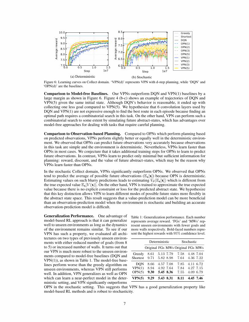
0.0 0.5 1.0 1.5Step 1e7

7.0

7.5

8.0

8.5

9.0

9.5

10.0

Avera

ge r

ew

ard

(a) Deterministic

0.0 0.5 1.0 1.5Step 1e7

6.0

6.5

7.0

7.5

8.0

8.5

Avera

ge r

ew

ard

(b) Stochastic

GreedyShortestDQNOPN(1)OPN(2)OPN(3)OPN(5)VPN(1)VPN(2)VPN(3)VPN(5)

Figure 6: Learning curves on Collect domain. ‘VPN(d)’ represents VPN with d-step planning, while ‘DQN’ and‘OPN(d)’ are the baselines.

Comparison to Model-free Baselines. Our VPNs outperform DQN and VPN(1) baselines by alarge margin as shown in Figure 6. Figure 4 (b-c) shows an example of trajectories of DQN andVPN(5) given the same initial state. Although DQN’s behavior is reasonable, it ended up withcollecting one less goal compared to VPN(5). We hypothesize that 6 convolution layers used byDQN and VPN(1) are not expressive enough to find the best route in each episode because finding anoptimal path requires a combinatorial search in this task. On the other hand, VPN can perform such acombinatorial search to some extent by simulating future abstract-states, which has advantages overmodel-free approaches for dealing with tasks that require careful planning.

Comparison to Observation-based Planning. Compared to OPNs which perform planning basedon predicted observations, VPNs perform slightly better or equally well in the deterministic environ-ment. We observed that OPNs can predict future observations very accurately because observationsin this task are simple and the environment is deterministic. Nevertheless, VPNs learn faster thanOPNs in most cases. We conjecture that it takes additional training steps for OPNs to learn to predictfuture observations. In contrast, VPNs learn to predict only minimal but sufficient information forplanning: reward, discount, and the value of future abstract-states, which may be the reason whyVPNs learn faster than OPNs.

In the stochastic Collect domain, VPNs significantly outperform OPNs. We observed that OPNstend to predict the average of possible future observations (Ex[x]) because OPN is deterministic.Estimating values on such blurry predictions leads to estimating Vθ(Ex[x]) which is different fromthe true expected value Ex[V (x)]. On the other hand, VPN is trained to approximate the true expectedvalue because there is no explicit constraint or loss for the predicted abstract state. We hypothesizethat this key distinction allows VPN to learn different modes of possible future states more flexibly inthe abstract state space. This result suggests that a value-prediction model can be more beneficialthan an observation-prediction model when the environment is stochastic and building an accurateobservation-prediction model is difficult.

Table 1: Generalization performance. Each numberrepresents average reward. ‘FGs’ and ‘MWs’ rep-resent unseen environments with fewer goals andmore walls respectively. Bold-faced numbers repre-sent the highest rewards with 95% confidence level.

Deterministic Stochastic

Original FGs MWs Original FGs MWs

Greedy 8.61 5.13 7.79 7.58 4.48 7.04Shortest 9.71 5.82 8.98 7.64 4.36 7.22

DQN 8.66 4.57 7.08 7.85 4.11 6.72VPN(1) 8.94 4.92 7.64 7.84 4.27 7.15OPN(5) 9.30 5.45 8.36 7.55 4.09 6.79

VPN(5) 9.29 5.43 8.31 8.11 4.45 7.46

Generalization Performance. One advantage ofmodel-based RL approach is that it can generalizewell to unseen environments as long as the dynamicsof the environment remains similar. To see if ourVPN has such a property, we evaluated all archi-tectures on two types of previously unseen environ-ments with either reduced number of goals (from 8to 5) or increased number of walls. It turns out thatour VPN is much more robust to the unseen environ-ments compared to model-free baselines (DQN andVPN(1)), as shown in Table 1. The model-free base-lines perform worse than the greedy algorithm onunseen environments, whereas VPN still performswell. In addition, VPN generalizes as well as OPNwhich can learn a near-perfect model in the deter-ministic setting, and VPN significantly outperformsOPN in the stochastic setting. This suggests that VPN has a good generalization property likemodel-based RL methods and is robust to stochasticity.

7

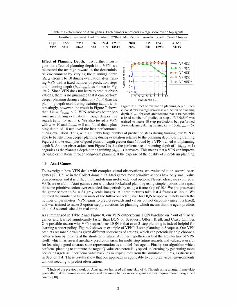
Table 2: Performance on Atari games. Each number represents average score over 5 top agents.

Frostbite Seaquest Enduro Alien Q*Bert Ms. Pacman Amidar Krull Crazy Climber

DQN 3058 2951 326 1804 12592 2804 535 12438 41658VPN 3811 5628 382 1429 14517 2689 641 15930 54119

1 2 3 4 5 6 7 8 9 10Plan depth (dtest)

−2

0

2

4

6

8

10

Avera

ge r

ew

ard

VPN(1)VPN(2)VPN(3)VPN(5)VPN(5)*

Figure 7: Effect of evaluation planning depth. Eachcurve shows average reward as a function of planningdepth, dtest, for each architecture that is trained witha fixed number of prediction steps. ‘VPN(5)*’ wastrained to make 10-step predictions but performed5-step planning during training (k = 10, dtrain = 5).

Effect of Planning Depth. To further investi-gate the effect of planning depth in a VPN, wemeasured the average reward in the determinis-tic environment by varying the planning depth(dtest) from 1 to 10 during evaluation after train-ing VPN with a fixed number of prediction stepsand planning depth (k, dtrain), as shown in Fig-ure 7. Since VPN does not learn to predict obser-vations, there is no guarantee that it can performdeeper planning during evaluation (dtest) than theplanning depth used during training (dtrain). In-terestingly, however, the result in Figure 7 showsthat if k = dtrain > 2, VPN achieves better per-formance during evaluation through deeper treesearch (dtest > dtrain). We also tested a VPNwith k = 10 and dtrain = 5 and found that a plan-ning depth of 10 achieved the best performanceduring evaluation. Thus, with a suitably large number of prediction steps during training, our VPN isable to benefit from deeper planning during evaluation relative to the planning depth during training.Figure 5 shows examples of good plans of length greater than 5 found by a VPN trained with planningdepth 5. Another observation from Figure 7 is that the performance of planning depth of 1 (dtest = 1)degrades as the planning depth during training (dtrain) increases. This means that a VPN can improveits value estimations through long-term planning at the expense of the quality of short-term planning.

4.3 Atari Games

To investigate how VPN deals with complex visual observations, we evaluated it on several Atarigames [2]. Unlike in the Collect domain, in Atari games most primitive actions have only small valueconsequences and it is difficult to hand-design useful extended options. Nevertheless, we explored ifVPNs are useful in Atari games even with short-lookahead planning using simple options that repeatthe same primitive action over extended time periods by using a frame-skip of 10.3 We pre-processedthe game screen to 84 × 84 gray-scale images. All architectures take last 4 frames as input. Wedoubled the number of hidden units of the fully-connected layer for DQN to approximately match thenumber of parameters. VPN learns to predict rewards and values but not discount (since it is fixed),and was trained to make 3-option-step predictions for planning which means that the agent predictsup to 0.5 seconds ahead in real-time.

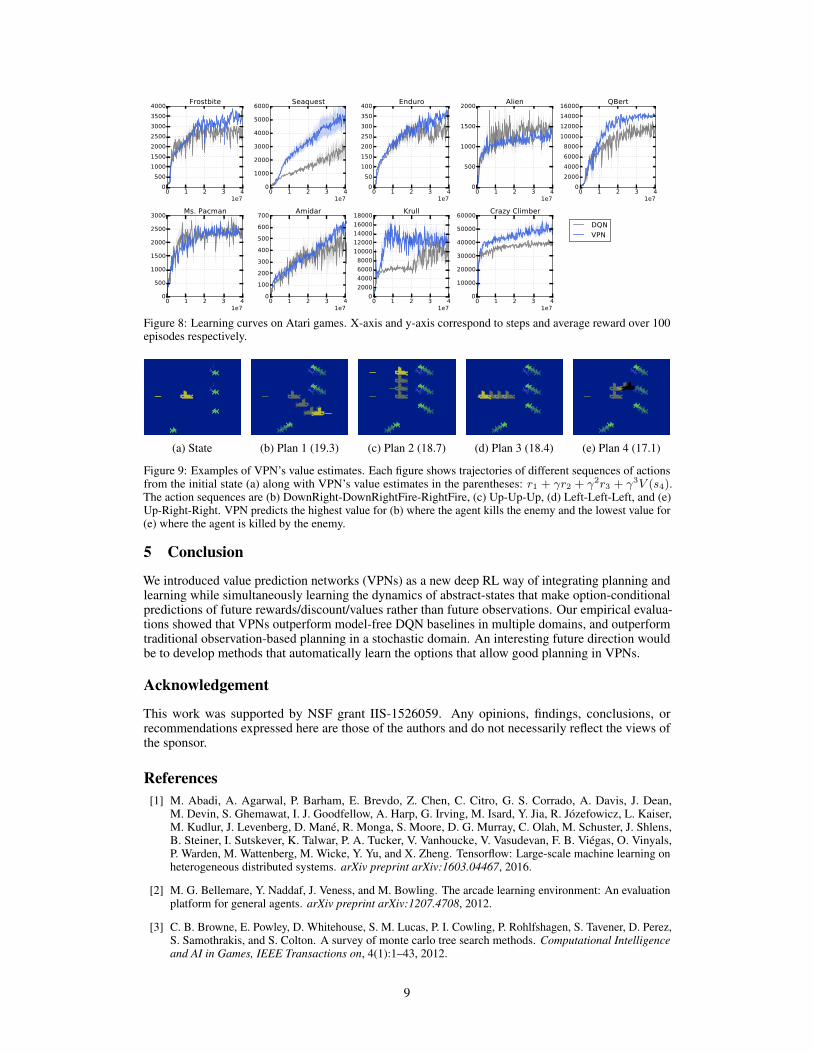
As summarized in Table 2 and Figure 8, our VPN outperforms DQN baseline on 7 out of 9 Atarigames and learned significantly faster than DQN on Seaquest, QBert, Krull, and Crazy Climber.One possible reason why VPN outperforms DQN is that even 3-step planning is indeed helpful forlearning a better policy. Figure 9 shows an example of VPN’s 3-step planning in Seaquest. Our VPNpredicts reasonable values given different sequences of actions, which can potentially help choose abetter action by looking at the short-term future. Another hypothesis is that the architecture of VPNitself, which has several auxiliary prediction tasks for multi-step future rewards and values, is usefulfor learning a good abstract-state representation as a model-free agent. Finally, our algorithm whichperforms planning to compute the target Q-value can potentially speed up learning by generating moreaccurate targets as it performs value backups multiple times from the simulated futures, as discussedin Section 3.4. These results show that our approach is applicable to complex visual environmentswithout needing to predict observations.

3Much of the previous work on Atari games has used a frame-skip of 4. Though using a larger frame-skipgenerally makes training easier, it may make training harder in some games if they require more fine-grainedcontrol [18].

8

0 1 2 3 41e7

0

500

1000

1500

2000

2500

3000

3500

4000Frostbite

0 1 2 3 41e7

0

1000

2000

3000

4000

5000

6000Seaquest

0 1 2 3 41e7

0

50

100

150

200

250

300

350

400Enduro

0 1 2 3 41e7

0

500

1000

1500

2000Alien

0 1 2 3 41e7

0

2000

4000

6000

8000

10000

12000

14000

16000QBert

0 1 2 3 41e7

0

500

1000

1500

2000

2500

3000Ms. Pacman

0 1 2 3 41e7

0

100

200

300

400

500

600

700Amidar

0 1 2 3 41e7

0

2000

4000

6000

8000

10000

12000

14000

16000

18000Krull

0 1 2 3 41e7

0

10000

20000

30000

40000

50000

60000Crazy Climber

DQNVPN

Figure 8: Learning curves on Atari games. X-axis and y-axis correspond to steps and average reward over 100episodes respectively.

(a) State (b) Plan 1 (19.3) (c) Plan 2 (18.7) (d) Plan 3 (18.4) (e) Plan 4 (17.1)

Figure 9: Examples of VPN’s value estimates. Each figure shows trajectories of different sequences of actionsfrom the initial state (a) along with VPN’s value estimates in the parentheses: r1 + γr2 + γ2r3 + γ3V (s4).The action sequences are (b) DownRight-DownRightFire-RightFire, (c) Up-Up-Up, (d) Left-Left-Left, and (e)Up-Right-Right. VPN predicts the highest value for (b) where the agent kills the enemy and the lowest value for(e) where the agent is killed by the enemy.

5 Conclusion

We introduced value prediction networks (VPNs) as a new deep RL way of integrating planning andlearning while simultaneously learning the dynamics of abstract-states that make option-conditionalpredictions of future rewards/discount/values rather than future observations. Our empirical evalua-tions showed that VPNs outperform model-free DQN baselines in multiple domains, and outperformtraditional observation-based planning in a stochastic domain. An interesting future direction wouldbe to develop methods that automatically learn the options that allow good planning in VPNs.

Acknowledgement

This work was supported by NSF grant IIS-1526059. Any opinions, findings, conclusions, orrecommendations expressed here are those of the authors and do not necessarily reflect the views ofthe sponsor.

References[1] M. Abadi, A. Agarwal, P. Barham, E. Brevdo, Z. Chen, C. Citro, G. S. Corrado, A. Davis, J. Dean,

M. Devin, S. Ghemawat, I. J. Goodfellow, A. Harp, G. Irving, M. Isard, Y. Jia, R. Józefowicz, L. Kaiser,M. Kudlur, J. Levenberg, D. Mané, R. Monga, S. Moore, D. G. Murray, C. Olah, M. Schuster, J. Shlens,B. Steiner, I. Sutskever, K. Talwar, P. A. Tucker, V. Vanhoucke, V. Vasudevan, F. B. Viégas, O. Vinyals,P. Warden, M. Wattenberg, M. Wicke, Y. Yu, and X. Zheng. Tensorflow: Large-scale machine learning onheterogeneous distributed systems. arXiv preprint arXiv:1603.04467, 2016.

[2] M. G. Bellemare, Y. Naddaf, J. Veness, and M. Bowling. The arcade learning environment: An evaluationplatform for general agents. arXiv preprint arXiv:1207.4708, 2012.

[3] C. B. Browne, E. Powley, D. Whitehouse, S. M. Lucas, P. I. Cowling, P. Rohlfshagen, S. Tavener, D. Perez,S. Samothrakis, and S. Colton. A survey of monte carlo tree search methods. Computational Intelligenceand AI in Games, IEEE Transactions on, 4(1):1–43, 2012.

9

[4] S. Chiappa, S. Racaniere, D. Wierstra, and S. Mohamed. Recurrent environment simulators. In ICLR,2017.

[5] D.-A. Clevert, T. Unterthiner, and S. Hochreiter. Fast and accurate deep network learning by exponentiallinear units (ELUs). arXiv preprint arXiv:1511.07289, 2015.

[6] C. Finn, I. J. Goodfellow, and S. Levine. Unsupervised learning for physical interaction through videoprediction. In NIPS, 2016.

[7] C. Finn and S. Levine. Deep visual foresight for planning robot motion. In ICRA, 2017.

[8] S. Gu, T. P. Lillicrap, I. Sutskever, and S. Levine. Continuous deep q-learning with model-based acceleration.In ICML, 2016.

[9] X. Guo, S. P. Singh, R. L. Lewis, and H. Lee. Deep learning for reward design to improve monte carlo treesearch in atari games. In IJCAI, 2016.

[10] M. Hausknecht and P. Stone. Deep recurrent q-learning for partially observable MDPs. arXiv preprintarXiv:1507.06527, 2015.

[11] K. He, X. Zhang, S. Ren, and J. Sun. Deep residual learning for image recognition. In CVPR, 2016.

[12] N. Heess, G. Wayne, D. Silver, T. P. Lillicrap, Y. Tassa, and T. Erez. Learning continuous control policiesby stochastic value gradients. In NIPS, 2015.

[13] M. Jaderberg, V. Mnih, W. Czarnecki, T. Schaul, J. Z. Leibo, D. Silver, and K. Kavukcuoglu. Reinforcementlearning with unsupervised auxiliary tasks. In ICLR, 2017.

[14] N. Kalchbrenner, A. van den Oord, K. Simonyan, I. Danihelka, O. Vinyals, A. Graves, and K. Kavukcuoglu.Video pixel networks. arXiv preprint arXiv:1610.00527, 2016.

[15] D. P. Kingma and J. Ba. Adam: A method for stochastic optimization. In ICLR, 2015.

[16] L. Kocsis and C. Szepesvári. Bandit based monte-carlo planning. In ECML, 2006.

[17] T. D. Kulkarni, A. Saeedi, S. Gautam, and S. Gershman. Deep successor reinforcement learning. arXivpreprint arXiv:1606.02396, 2016.

[18] A. S. Lakshminarayanan, S. Sharma, and B. Ravindran. Dynamic action repetition for deep reinforcementlearning. In AAAI, 2017.

[19] I. Lenz, R. A. Knepper, and A. Saxena. DeepMPC: Learning deep latent features for model predictivecontrol. In RSS, 2015.

[20] N. Mishra, P. Abbeel, and I. Mordatch. Prediction and control with temporal segment models. In ICML,2017.

[21] V. Mnih, A. P. Badia, M. Mirza, A. Graves, T. P. Lillicrap, T. Harley, D. Silver, and K. Kavukcuoglu.Asynchronous methods for deep reinforcement learning. In ICML, 2016.

[22] V. Mnih, K. Kavukcuoglu, D. Silver, A. A. Rusu, J. Veness, M. G. Bellemare, A. Graves, M. Riedmiller,A. K. Fidjeland, G. Ostrovski, S. Petersen, C. Beattie, A. Sadik, I. Antonoglou, H. King, D. Kumaran,D. Wierstra, S. Legg, and D. Hassabis. Human-level control through deep reinforcement learning. Nature,518(7540):529–533, 2015.

[23] J. Oh, V. Chockalingam, S. Singh, and H. Lee. Control of memory, active perception, and action inminecraft. In ICML, 2016.

[24] J. Oh, X. Guo, H. Lee, R. L. Lewis, and S. Singh. Action-conditional video prediction using deep networksin atari games. In NIPS, 2015.

[25] E. Parisotto and R. Salakhutdinov. Neural map: Structured memory for deep reinforcement learning. arXivpreprint arXiv:1702.08360, 2017.

[26] D. Precup. Temporal abstraction in reinforcement learning. PhD thesis, University of Massachusetts,Amherst, 2000.

[27] T. Raiko and M. Tornio. Variational bayesian learning of nonlinear hidden state-space models for modelpredictive control. Neurocomputing, 72(16):3704–3712, 2009.

10

[28] D. Silver, A. Huang, C. J. Maddison, A. Guez, L. Sifre, G. van den Driessche, J. Schrittwieser,I. Antonoglou, V. Panneershelvam, M. Lanctot, S. Dieleman, D. Grewe, J. Nham, N. Kalchbrenner,I. Sutskever, T. Lillicrap, M. Leach, K. Kavukcuoglu, T. Graepel, and D. Hassabis. Mastering the game ofgo with deep neural networks and tree search. Nature, 529(7587):484–489, 2016.

[29] D. Silver, R. S. Sutton, and M. Müller. Temporal-difference search in computer go. Machine Learning,87:183–219, 2012.

[30] D. Silver, H. van Hasselt, M. Hessel, T. Schaul, A. Guez, T. Harley, G. Dulac-Arnold, D. Reichert,N. Rabinowitz, A. Barreto, and T. Degris. The predictron: End-to-end learning and planning. In ICML,2017.

[31] B. C. Stadie, S. Levine, and P. Abbeel. Incentivizing exploration in reinforcement learning with deeppredictive models. arXiv preprint arXiv:1507.00814, 2015.

[32] M. Stolle and D. Precup. Learning options in reinforcement learning. In SARA, 2002.

[33] R. S. Sutton. Integrated architectures for learning, planning, and reacting based on approximating dynamicprogramming. In ICML, 1990.

[34] R. S. Sutton, D. Precup, and S. Singh. Between MDPs and semi-MDPs: A framework for temporalabstraction in reinforcement learning. Artificial intelligence, 112(1):181–211, 1999.

[35] R. S. Sutton, C. Szepesvári, A. Geramifard, and M. H. Bowling. Dyna-style planning with linear functionapproximation and prioritized sweeping. In UAI, 2008.

[36] A. Tamar, S. Levine, P. Abbeel, Y. Wu, and G. Thomas. Value iteration networks. In NIPS, 2016.

[37] A. Vezhnevets, V. Mnih, S. Osindero, A. Graves, O. Vinyals, J. Agapiou, and K. Kavukcuoglu. Strategicattentive writer for learning macro-actions. In NIPS, 2016.

[38] Z. Wang, T. Schaul, M. Hessel, H. van Hasselt, M. Lanctot, and N. de Freitas. Dueling network architecturesfor deep reinforcement learning. In ICML, 2016.

[39] C. J. Watkins and P. Dayan. Q-learning. Machine learning, 8(3-4):279–292, 1992.

[40] H. Yao, S. Bhatnagar, D. Diao, R. S. Sutton, and C. Szepesvári. Multi-step Dyna planning for policyevaluation and control. In NIPS, 2009.

11

A Comparison between VPN and DQN in the Deterministic Collect

Observation DQN’s trajectory VPN’s trajectory VPN’s 10-step plan

Figure 10: Examples of trajectories and planning on the deterministic Collect domain. The first column showsinitial observations, and the following two columns show trajectories of DQN and VPN respectively. It is shownthat DQN sometimes chooses a non-optimal option and ends up with collecting fewer goals than VPN. The lastcolumn visualizes VPN’s 10 option-step planning from the initial state. Note that VPN’s initial plans do notalways match with its actual trajectories because the VPN re-plans at every step as it observes its new state.

12

B Comparison between VPN and OPN in the Stochastic Collect

OPN

VPN

OPN

VPN

OPN

VPN

t = 1 t = 2 t = 3 t = 4 t = 5 t = 6 t = 7

t = 8 t = 9 t = 10 t = 11 t = 12 t = 13 t = 14

t = 15 t = 16 t = 17 t = 18 t = 19 t = 20

Figure 11: Example of trajectory on the stochastic Collect domain. Each row shows a trajectory of VPN (top)and OPN (bottom) given the same initial state. At t=6, the VPN decides to move up to collect nearby goals,while the OPN moves left to collect the other goals. As a result, the OPN collects two fewer goals compared toVPN. Since goals move randomly and the outcome of option is stochastic, the agent should take into accountmany different possible futures to find the best option with the highest expected outcome. Though the outcomeis noisy due to the stochasticity of the environment, our VPN tends to make better decisions more often thanOPN does in expectation.

13

C Examples of Planning on Atari Games

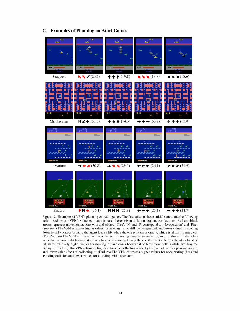
Figure 12: Examples of VPN’s planning on Atari games. The first column shows initial states, and the followingcolumns show our VPN’s value estimates in parentheses given different sequences of actions. Red and blackarrows represent movement actions with and without ‘Fire’. ‘N’ and ‘F’ correspond to ‘No-operation’ and ‘Fire’.(Seaquest) The VPN estimates higher values for moving up to refill the oxygen tank and lower values for movingdown to kill enemies because the agent loses a life when the oxygen tank is empty, which is almost running out.(Ms. Pacman) The VPN estimates the lowest value for moving towards an enemy (ghost). It also estimates a lowvalue for moving right because it already has eaten some yellow pellets on the right side. On the other hand, itestimates relatively higher values for moving left and down because it collects more pellets while avoiding theenemy. (Frostbite) The VPN estimates higher values for collecting a nearby fish, which gives a positive reward,and lower values for not collecting it. (Enduro) The VPN estimates higher values for accelerating (fire) andavoiding collision and lower values for colliding with other cars.

14

D Details of Learning

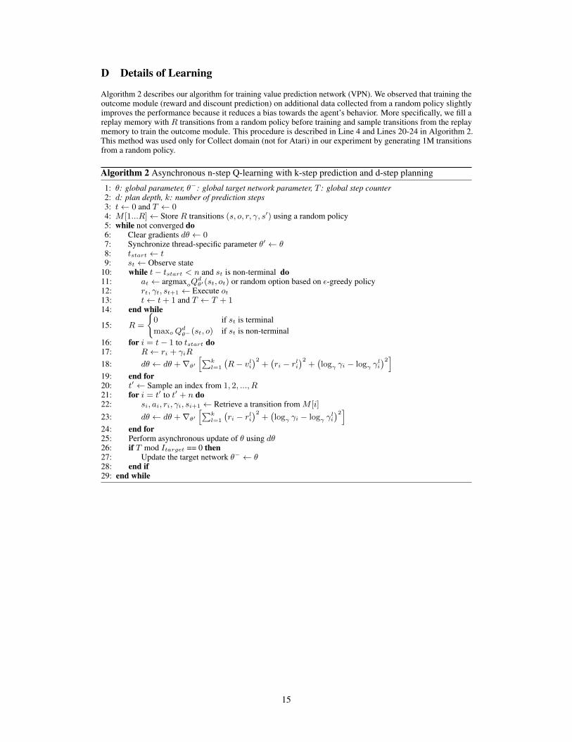
Algorithm 2 describes our algorithm for training value prediction network (VPN). We observed that training theoutcome module (reward and discount prediction) on additional data collected from a random policy slightlyimproves the performance because it reduces a bias towards the agent’s behavior. More specifically, we fill areplay memory with R transitions from a random policy before training and sample transitions from the replaymemory to train the outcome module. This procedure is described in Line 4 and Lines 20-24 in Algorithm 2.This method was used only for Collect domain (not for Atari) in our experiment by generating 1M transitionsfrom a random policy.

Algorithm 2 Asynchronous n-step Q-learning with k-step prediction and d-step planning

1: θ: global parameter, θ−: global target network parameter, T : global step counter2: d: plan depth, k: number of prediction steps3: t← 0 and T ← 04: M [1...R]← Store R transitions (s, o, r, γ, s′) using a random policy5: while not converged do6: Clear gradients dθ ← 07: Synchronize thread-specific parameter θ′ ← θ8: tstart ← t9: st ← Observe state

10: while t− tstart < n and st is non-terminal do11: at ← argmaxoQ

dθ′(st, ot) or random option based on ε-greedy policy

12: rt, γt, st+1 ← Execute ot13: t← t+ 1 and T ← T + 114: end while

15: R =

{0 if st is terminalmaxoQ

dθ−(st, o) if st is non-terminal

16: for i = t− 1 to tstart do17: R← ri + γiR

18: dθ ← dθ +∇θ′[∑k

l=1

(R− vli

)2+(ri − rli

)2+(logγ γi − logγ γ

li

)2]19: end for20: t′ ← Sample an index from 1, 2, ..., R21: for i = t′ to t′ + n do22: si, ai, ri, γi, si+1 ← Retrieve a transition from M [i]

23: dθ ← dθ +∇θ′[∑k

l=1

(ri − rli

)2+(logγ γi − logγ γ

li

)2]24: end for25: Perform asynchronous update of θ using dθ26: if T mod Itarget == 0 then27: Update the target network θ− ← θ28: end if29: end while

15

E Details of Hyperparameters

Figure 13: Transition module used for Collect domain. The first convolution layer uses different weightsdepending on the given option. Sigmoid activation function is used for the last 1x1 convolution such that itsoutput forms a mask. This mask is multiplied to the output from the 3rd convolution layer. Note that there is aresidual connection from s to s′. Thus, the transition module learns the change of the consecutive abstract states.

E.1 Collect

The encoding module of our VPN consists of Conv(32-3x3-1)-Conv(32-3x3-1)-Conv(64-4x4-2) where Conv(N-KxK-S) represents N filters with size of KxK with a stride of S. The transition module is illustrated in Figure 13.It consists of OptionConv(64-3x3-1)-Conv(64-3x3-1)-Conv(64-3x3-1) and a separate Conv(64-1x1-1) for themask which is multiplied to the output of the 3rd convolution layer of the transition module. ‘OptionConv’uses different convolution weights depending on the given option. We also used a residual connection from theprevious abstract state to the next abstract state such that the transition module learns the difference between twostates. The outcome module has OptionConv(64-3x3-1)-Conv(64-3x3-1)-FC(64)-FC(2) where FC(N) representsa fully-connected layer with N hidden units. The value module consists of FC(64)-FC(1). Exponential linearunit (ELU) [5] was used as an activation function for all architectures.

Our DQN baseline consists of the encoding module followed by the transition module followed by the valuemodule. Thus, the overall architecture is very similar to VPN except that it does not have the outcome module.To match the number of parameters, we used 256 hidden units for DQN’s value module. We found that thisarchitecture outperforms the original DQN architecture [22] on Collect domain and several Atari games.

The model network of OPN baseline has the same architecture as VPN except that it has an additional decodingmodule which consists of Deconv(64-4x4-2)-Deconv(32-3x3-1)-Deconv(32-3x3-1). This module is applied tothe predicted abstract-state so that it can predict the future observations. The value network of OPN has the samearchitecture as our DQN baseline.

A discount factor of 0.98 was used, and the target network was synchronized after every 10K steps. The epsilonfor ε-greedy policy was linearly decreased from 1 to 0.05 for the first 1M steps.

E.2 Atari Games

The encoding module consists of Conv(16-8x8-4)-Conv(32-4x4-2), and the transition module has OptionConv(32-3x3-1)-Conv(32-3x3-1) with a mask and a residual connection as described above. The outcome module hasOptionConv(32-3x3-1)-Conv(32-3x3-1)-FC(128)-FC(1), and the value module consists of FC(128)-FC(1). TheDQN baseline has the same encoding module followed by the transition module and the value module, and weused 256 hidden units for the value module of DQN to approximately match the number of parameters. Theother hyperparameters are same as the ones used in the Collect domain except that a discount factor of 0.99 wasused.

16