value enhancing capital budgeting and firm-specific stock returns variation
TRANSCRIPT

First draft: September 1st, 1999 This draft: October 8th 2001 Comments Welcome
Value Enhancing Capital Budgeting and Firm-Specific Stock Returns Variation
Artyom Durnev*, Randall Morck**, and Bernard Yeung***
* Graduate Student, University of Michigan Business School, Ann Arbor, MI 48109. Tel: (734) 763-6126. E-mail: [email protected]. ** Stephen A. Jarislowsky Distinguished Professor of Finance, Faculty of Business, University of Alberta, Edmonton, Alberta, Canada, T6G 2R6. Tel: (780) 492-5683. E-mail [email protected]; Research Associate, National Bureau of Economic Research, 1050 Massachusetts Avenue, Cambridge, MA 02138 USA. *** Abraham Krasnoff Professor of International Business and Professor of Economics, Stern School of Business, New York University, New York, NY 10012. Tel: (212) 998-0425. Fax: (212) 995-4221. E-mail [email protected]. We are grateful for helpful comments by Yakov Amihud, Serdar Dinc, Bjørne Jørgensen, Han Kim, Claudio Loderer, Roberta Romano, Andrei Shleifer, Richard Sloan, Jeremy Stein, and Larry White; and to participants at the NBER Corporate Finance Seminar, le Centre Interuniversitaire de Recherche en Analyse des Organisations (CIRANO) in Montreal, the European Financial Management Association meeting in Lugano, Baruch-CUNY, Columbia Business School, Indiana University, the University of Michigan, MIT Sloan School, New York University, the University of North Carolina, and the University of Chicago; and to students in Andrei Shleifer’s Research Seminar on Behavioral Finance at Harvard.

1
Value Enhancing Capital Budgeting and Firm-Specific Stock Returns Variation
Artyom Durnev, Randall Morck, and Bernard Yeung
Abstract A major issue in corporate finance is the extent to which managers’ decisions enhance firm
value. We show that capital budgeting decisions are more consistent with value maximization in
industries whose stocks exhibit greater firm-specific return variation. This finding argues against
the view that firm-specific return variation is noise, and supports Roll’s (1988) view that firm-
specific return variation indicates activity by risk arbitrageurs. Given this, we argue that
corporate investment decisions tend to be more firm value enhancing where firm-specific risk
arbitrage activity is greater.
1. Introduction
It is plausible that the extent to which stock prices approximate fundamental (full
information) values is related to the extent to which corporate capital budgeting decisions
enhance firm market value. First, stock prices play critical signaling and incentive alignment
roles in many corporate governance mechanisms that can curb the sorts of self-serving or inept
managerial behavior that lead to non-value-maximizing capital budgeting decisions.1 For
example, shareholder derivative lawsuits, executive stock options, and the market for corporate
control all depend upon the efficiency of the stock market as an information processor. Second,
stock prices convey information about investors’ perceptions to managers. Stock price reactions
to managers’ decisions can provide useful feedback that improves corporate governance (and so
1 See e.g. Amihud and Lev (1981), Shleifer and Vishny (1989), Jensen (1986). See Stein (2001) for a survey.

2
capital budgeting) if shareholders are well informed. Third, the more informed investors are, the
easier it is for managers to raise external financing to fund value-enhancing projects.
Thus, a higher incidence of value enhancing corporate capital budgeting decisions should
be evident where stock prices are better informed, by which we mean that a greater fraction of
public and private information is capitalized into the stock price. To empirically examine this
proposition requires two steps:
First, we need a measure of how informed stock prices are. To do this, we follow Roll
(1988) and distinguish firm-specific returns variation from market-related and industry-related
returns variation. Roll shows that common asset pricing models have low R2 statistics because
of high firms-specific return variation not associated with public information. He argues that
“the financial press misses a great deal of relevant information generated privately” (p. 564), and
concludes that this firm-specific returns variation reflects the capitalization of private
information into share prices as a result of informed trading by risk arbitrageurs. However, he
concedes (p. 56) that firm-specific returns variation might reflect “either private information or
else occasional frenzy unrelated to concrete information.”
If firm-specific returns variation reflects investor frenzy, it is larger when prices are less
informed. If firm-specific returns variation reflects the capitalization of private firm-specific
information, several possibilities arise. First, greater firm-specific variation might again reflect
less informed pricing because mispricing must exist to attract arbitrageurs. Second, greater firm-
specific variation might be unrelated to how informed stock prices are because arbitrageur
activity keeps all stock prices roughly equally informed. Third, greater firm-specific variation
might reflect more informed pricing, perhaps because the presence of informed arbitrageurs
reduces the influence of noise traders, as in De Long et al. (1986).

3
Second, we require a measure of the extent to which corporate capital budgeting
decisions enhance firm market value. To achieve that, we directly estimate Tobin’s marginal q
ratios, one plus the net present value (NPV) of the firm’s marginal capital budgeting project over
its set-up cost, all as perceived by investors. The deviation of Tobin’s marginal q, based on firm
market value, from its optimal level (which is one when tax factors are ignored) measures the
extent to which firms’ capital budgeting decisions enhance firm market value.
We find highly significant and robust empirical evidence that greater firm-specific stock
return variation is associated with marginal q ratios closer to its optimal level. This finding is
consistent with the joint hypothesis that more informed stock prices are associated with capital
budgeting more aligned to market value maximization and that greater firm-specific stock returns
variation is indicative of more informed stock prices. That is, high firm-specific returns
variation, far from reflecting investor frenzy, signifies the capitalization of private information
into stock prices through risk arbitrage trading, which leads to more informed, rather than less
informed, stock prices.
Section 2 explains our firm specific stock return variation variables, while section 3
explains our measure of the quality of corporate capital budgeting decisions. Section 4 describes
our empirical estimation techniques and our main control variables. Section 5 presents our
empirical results, and section 6 reports robustness checks. Section 7 discusses our results and
section 8 concludes. The appendix contains details about the construction of our data and a
complete description of our marginal q estimation technique.

4
2. Firm-Specific Returns Variation
2.1 Motivation
Information about fundamentals is capitalized into stock prices via two channels: a
general revaluation of stock values following the release of public information (such as Fed
interest rate announcements or SEC filings), and the trading activity of risk arbitrageurs who
gather and possess private information. Shleifer and Vishny (1997a) argue that risk arbitrage is
limited, and may be more limited in some circumstances than others.
Roll (1988) concludes that firm-specific return variation could reflect either the
capitalization of private information into stock prices by informed risk arbitrageurs or investor
frenzy. Current evidence suggests that Roll’s former interpretation is more plausible.
First, Figure 1 shows the average R2 statistics of regressions of firm-level stock returns on
local and US market returns using 1995 data for a range of countries, as reported by Morck et al.
(2000). These R2s are very low for countries with well-developed financial systems, such as the
United States, Canada, and the United Kingdom; but are very high for emerging markets such as
Poland and China. Morck et al. (2000) show that these results are clearly not due to differences
in country or market size, and that they are unlikely to be due to more synchronous fundamentals
in emerging economies. They propose that low average market model R2s reflect greater activity
by the risk arbitrageurs Roll (1988) posits as responsible for firm-specific price movements, and
conjecture that a low market model R2 may actually mark a more efficient stock market.
Second, Durnev et al. (2001) show that stock returns more accurately predict future
earnings changes in industries where returns are less synchronous, as measured by a market
model R2 statistic. Collins et al. (1987) and others in the accounting literature regard such
predictive power as gauging the ‘information content’ of stock prices. In this sense, stock prices

5
have a higher information content when firm-specific variation is a larger fraction of total
variation.
Finally, Wurgler (2000) shows that capital flows are more responsive to changes in
value-added in countries exhibiting less synchronous stock returns. This suggests that capital
moves more quickly to its highest value uses in countries whose stocks move asynchronously.
That is, stock markets in which firm-specific variation is a larger fraction of total variation are
more functionally efficient in the sense of Tobin (1982).
We nonetheless retain an ecumenical attitude, and allow the data to suggest the best
interpretation of firm-specific returns variation.
2.2 Measuring Firm-Specific Returns Variation
This section describes the estimation of our firm-specific return variation measures. Its
contents are summarized in Table 1. The data used in this estimation procedure are daily total
returns for 1990 through 1992 for the 6,021 firms for which both CRSP and Compustat data
exist. These firms span 214 three-digit SIC industries. The construction of the dataset is
described in detail in the appendix.
We gauge firm-specific return variation by regressing the return of the stock of firm j in
industry i, ri,j,t, on market and industry returns, rm,t and ri,t.
r r ri j t j j m m t j i i t i j t, , , , , , , , ,= + + +β β β ε0 [1]
for each firm j in industry i, where t is a daily time index over the period from 1990 through
1992, ri j t, , is firm j’s stock return, rm t, is a market return, and ri t, an industry return for industry i
(which contains firm j). The market index and industry indices in [1] are value-weighted
averages excluding the firm in question. This exclusion prevents spurious correlations between

6
firm returns and industry returns in industries that contain few firms. One minus the average R2
of regression [1] for all firms in an industry is a measure of the importance of firm-specific
return variation in that industry, and we interpret this as gauging the activity of risk arbitrageurs
capitalizing private information.
Although regression [1] resembles standard asset pricing equations, we do not emphasize
this. Our purpose is not to explain a relationship between returns and systematic risk, but to
understand the economic importance of firm-specific stock price variation. Stock price variation
associated with macroeconomic or industry information is of interest to us primarily as a control
variable. Note also that we depart from the standard terminology of asset pricing and follow
Roll (1988) in distinguishing ‘firm-specific’ variation from the sum of market-related and
industry-related variation. For simplicity, we refer to the latter sum as ‘systematic’ variation,
though this is not strictly correct. We decompose return variation in this way because Roll (1988)
specifically links arbitrage that capitalizes private information to firm-specific variation.
A standard variance decomposition lets us express an industry-average R2 as
Rim i
i m i
22
2 2=+
σσ σε
,
, ,, [2]
where
σ
σ
ε ,
,
,
,
i
i jj i
jj i
m i
i jj i
jj i
SSR
T
SSM
T
2
2
=
=
∈
∈
∈
∈
∑∑
∑∑
[3]

7
for SSRi,j and SSMi,j the unexplained and explained variations respectively of regression [1] for
firm j in industry i. As [3] indicates, the sums are scaled by the number of daily return
observations available in industry i, i.e., by Tjj i∈∑ .
Since σ ε ,i2 and σ m i,
2 have skewness coefficients of 5.31 and 5.30 respectively and kurtoses
of 40.7 and 36.7 respectively, we apply a logarithmic transformation. The distributions of
ln(σ ε ,i2 ) and ln(σ m i,
2 ) are both more symmetric (skewness coefficients of 0.16 and 0.52
respectively) and less leptokurtic (kurtoses of 4.11 and 4.59 respectively).
The distribution of 1 2− Ri is also negatively skewed (skewness = -0.91) and mildly
leptokurtic (kurtosis = 4.64). Moreover, it has the econometrically undesirable characteristic of
being bounded within the unit interval. As recommended by Theil (1971, chapter 12), we
circumvent the bounded nature of R2 by applying a logistic transformation
Ψii
i
RR
=−
ln 1 2
2 [4]
taking 1- Ri2 ∈ [0,1] to Ψi ∈ ℜ . We thus use the Greek letter psi to denote firm-specific stock
return variation measured relative to variations due to industry- and market-wide factors. The
transformed variable is again less skewed (skewness = 0.24) and less leptokurtic (kurtosis =
3.87). The hypothesis that Ψi is normally distributed cannot be rejected in a standard W-test (p-
value = 0.14).
The transformed variable Ψi also possesses the useful trait that
Ψ ii
i
i
m ii m i
RR
=−
=
= −ln ln ln( ) ln( ),
,, ,
1 2
2
2
22 2σ
σσ σε
ε [5]

8
Intuitively, the higher the value of Ψi, the more important is firm-specific variation, σ ε ,i2 ,
relative to market and industry-wide variation, σ m i,2 , in explaining the stock price movements of
firms in industry i.
In the following, we refer to ln(σ ε ,i2 ) as absolute firm-specific stock return variation,
ln(σ m i,2 ) as absolute systematic stock return variation, and Ψi as relative firm-specific stock
return variation.
Table 1 contains brief descriptions of these variables, and of all other variables used in
this study. Panel A of Table 2 shows the mean, standard deviation, minimum and maximum of
each measure of stock return variations: ln(σ ε ,i2 ), ln(σ m i,
2 ) and Ψi. The substantial standard
deviations of all three measures and the substantial difference between their minimum and
maximum values attest to their variation across industries. Higher firm-specific and systematic
stock return variations tend to occur together (ρ = 0.761, p-val = 0.00).2
3. Tobin’s Marginal q Ratio
3.1 Motivation
Optimal capital budgeting consists of undertaking all available projects with positive
expected net present value (NPV) and avoiding all those projects with negative expected NPV.
The NPV of a project is the present value of the net cash flows, cft, it will produce at all future
times t less its set up cost, C0. Thus, optimal capital budgeting requires undertaking projects if
and only if
2 In our sample, examples of high firm-specific stock return variation industries include: commercial sports, knitting mills, crude petroleum & natural gas, periodical publications, and tobacco. Examples of low firm-specific stock

9
( )E[ ] ENPVcf
rCt
tt
=+
−
>
=
∞
∑ 10
10 [6]
where E is the expectations operator. Under ordinary circumstances, managers are the decision
makers, and the E operator should be based on the manager’s information set.
To make the NPV of corporate capital expenditure comparable across firms, we scale by
set up costs to obtain a profitability index (PI). Optimal capital budgeting entails undertaking a
project if and only if its expected profitability index surpasses one.
( )E [ ] EE [ ]
mgt mgtt
tt
mgtPIC
cfr
NPVC
=+
= + >
=
∞
∑11
1 10 1 0
[7]
where we now explicitly use Emgt to denote management’s expectations.
The change in firm market value due to its (unexpected) capital expenditure equals
investors’ estimate of the NPV of the projects undertaken. The change in the value of a firm
associated with a unit increase in its stock of capital goods (replacement cost) is the firm’s
marginal Tobin’s q ratio, denoted
& E( )
E [ ],q
VK C
cfr
NPVCj t s
tt
t
s= =+
= +
=
∞
∑∆∆
11
10 1 0
[8]
where we redefine C0 to be the total setup cost of all projects undertaken this period, cft to be the
total cash flows those projects generate in future periods t, and Es to investors’ expectations.
In summary, market value maximizing corporate investment requires that managers
undertake all projects to which investors assign positive NPVs and no projects to which investors
assign negative NPVs. A firm that follows this strategy should have a Tobin’s marginal q ratio
approximately equal to one. Tax factors, discussed in more detail below, can cause value
return variation industries include engines and turbines, general building constructors, department stores, drug and proprietary stores, electric, gas and other services (regulated industries), and operative builders.

10
maximization to push marginal q’s towards a threshold value slightly different from one. We
account for tax factors in our empirical tests.
We wish to see in which industries marginal q, as depicted in [8], is close to its optimal
value. Where marginal q exceeds its optimal value, we may infer underinvestment. Likewise,
where marginal q is below its optimal value, we may infer overinvestment. We discuss reasons
why marginal q might differ from its value maximizing level in the next section. We now
explain our procedure for estimating marginal q.
3.2 Measuring Tobin’s Marginal q Ratio
To obtain reliable estimates of the impact of investment on firm market value, we must
use annual data. (Quarterly financial data are unaudited). If we used a long time window to
estimate our variables, it is likely that shifting technological constraints, market conditions, and
governance changes would make our estimates unreliable. Also, relying only on firms with data
available for many years creates a survival bias and makes our estimates unrepresentative of all
firms. We therefore pool cross-section and time-series data over the relatively short window
from 1993 to 1997 to construct more reliable industry-level marginal Tobin’s q ratio estimates.
To match this, our firm-specific stock return variation and control variables are also industry
average measures.
The estimation procedure we use to estimate marginal q ratios, as defined in [8], is
complicated, and a full description is provided in the appendix. The following is a brief
overview.
Our basic approach is to write the marginal q of firm j as the ratio

11
&( $ $ )
( $ $ ), ,
, ,
, , , ,
, , , ,
qV E VA E A
V V r d
A A gjj t t j t
j t t j t
j t j t j t j t
j t j t j t j t
=−−
=− + −
− + −−
−
−
−
1
1
1
1
1
1 δ [9]
where Vj,t and Aj,t are the market value (equity value plus debt value) and stock of capital goods
respectively of firm j at time t, and Et is the expectations operator using all information extant at
time t.3 The expected market value of the firm in period t is its market value in period t-1
augmented by the expected return from owning the firm, $ ,rj t , and its disbursements to investors,
which includes cash dividends, share repurchases, and interest expenses, $ ,d j t .4 The expected
value of the firm’s capital assets in period t is the value of its capital assets in period t-1
augmented by its expected rate of spending on capital goods, $ ,g j t and the expected depreciation
rate on those capital goods, $ ,δ j t .
Cross multiplying and simplifying [9] leads to
V V
Aq g q
A AA
rVA
divA
j t j t
j tj j j j
j t j t
j tj
j t
j tj
j t
j t
, ,
,
, ,
,
,
,
,
,
& ( ) &−
= − − +−
+ −−
−
−
−
−
−
−
−
1
1
1
1
1
1
1
1δ ξ [10]
where ξj is a tax wedge measure.5
We can estimate [10] as a regression
∆ ∆VA
AA
VA
divA
uj ti
j ti
i i j ti
j ti
i j ti
j ti
i j ti
j ti j t
i,
,
,
,
,
,
,
,,
− −
−
−
−
−
= + + +1
01
11
12
1
1
α β β β + [11]
3 An alternative approach would be to use equity value only as the numerator of marginal q. This would be consistent with the view that managers maximize shareholder value, rather than firm value, but ignores many legal requirements that managers consider creditors’ interests as well if bankruptcy is a reasonable possibility. Focusing on equity value also highlights the issue of whether managers should maximize the value of existing shareholders’ wealth or that of existing and new shareholders. We assume the latter and also add the value of creditors claims in [9], so that our implicit maximand is Vt rather than shareholder value. However, we shall point out later that the alternative approach leads to qualitatively similar results. 4 We can omit interest if debt is assumed to be perpetual so that periodic repayments do not affect the principal. Omitting interest expenses does not affect our results. Since we are calculating the return from owning the entire firm, not from owning a single share, stock repurchases must be included as part of cash payments to investors. 5 This relationship can also be derived as an Euler equation resulting from the firm’s intertemporal value maximization problem.

12
across all firms j in industry i at time t. We pool firm observations to estimate an industry
average marginal q ratio &qii≅ β0 for each of 214 three-digit nonfinancial industries i using 1993
to 1997 annual data. Details about the construction of this dataset and the precise econometric
specification of the regressions are presented in the appendix.
Summary statistics of our marginal Tobin’s q ratio estimates are presented in panel B of
Table 2. The average marginal q across our sample of industries is 0.69, with a standard
deviation of 0.64, a minimum value of -2.45 and a maximum value of 2.68. These estimates are
consistent with a prevalence of overinvestment in the US nonfinancial corporate sector in the
mid 1990s.
The average estimated values of β1i and β2
i are broadly consistent with their
interpretations in [10]. The average estimated coefficient β1i (the coefficient of lagged average
q) is 0.104, implying an average cost of capital of 10.4%. The average estimated value of β2i on
the disbursement rate is -0.799, and is insignificantly different from negative one at 10% level in
63 out of 214 industries. The average intercept, α δij j t j tq g= − −& ( ), , , is -0.048, and is
insignificantly different from zero at 10% level in 110 out of 214 industries.
Additional collaborative evidence adds credence to our marginal q estimates. The
regression coefficient α δij j t j tq g = − −& ( ), , is indeed negative and significantly correlated with
growth in physical capital. Also, β1i is indeed highly significantly positively correlated with
estimated weighted average costs of capital.
We are interested in whether firm-specific stock return variation is associated with the
distance of marginal q’s from its optimal value, which we temporarily assume to be one. We
measure the distance between &q and one as either ( &q -1)2, the square of marginal q minus one, or

13
as | &q -1|, the absolute value of marginal q minus one. The former metric places a heavier
weighting of extreme values of marginal q.
Summary statistics of &q , ( &q -1)2 and | &q -1| are therefore presented together in panel B of
Table 2. For ease of exposition, we shall refer to ( &q -1)2 and | &q -1| as measures of the quality of
capital budgeting decisions, though they are more properly regarded as measures of investors’
aggregated opinions about the quality of capital budgeting decisions.
4. Empirical Framework
4.1 Motivation
We wish to understand under what circumstances marginal q deviates from its market
value maximizing level. Three possibly overlapping cases are worthy of note.
4.1.1 Corporate Governance Problems
Marginal q can deviate from its value maximizing level because of agency problems.
Managers may distort capital budgeting policies in ways that advance their individual self-
interest, as modeled by Jensen and Meckling (1976), Shleifer and Vishny (1989), and others.
Managers might overinvest because of free cash flow problems, empire building, etc.; or they
might underinvest because they are exposed to firm-specific risk that diversified investors
ignore. Alternatively, managers may be ill informed or simply incompetent, and hence unable to
identify their firm’s optimal capital budgeting policy. Roll’s (1986) hypothesis, that hubris can
induce managers to overestimate their ability to generate positive NPVs, is an example of the
latter sort of agency problem.

14
A range of corporate governance mechanisms, surveyed by Shleifer and Vishny (1997b),
limits such agency problems. These include shareholder derivative lawsuits, executive stock
options, board oversight, hostile takeovers, institutional investors, and various other mechanisms
that align top managers’ incentives to value maximization. For example, shareholder derivative
lawsuits can be launched by any shareholder against managers whose decisions caused the value
of the firm to fall precipitously. Performance based compensations reward CEOs when their
stock price rises, boards sack CEOs when their firms’ stock underperforms the stocks of industry
peers, raiders launch takeovers of firms with sagging stock prices, and institutional investor
activism is often triggered by lagging share prices. Finally, feedback from the trades of informed
investors can cause ill-informed CEOs to learn.
These corporate governance mechanisms are most likely to function properly when share
prices are good estimates of fundamental values. Shareholder derivative lawsuits, proxy fights,
and hostile takeovers are all mechanisms that remove managers when the share price falls
unacceptably, so as to replace them with new managers who will better maximize the market
value of the firm. Performance based compensations reward managers when share prices rise,
so as to retain a value maximizing management team. Most obviously, share prices make the
most sense as a feedback mechanism when they include as much information as possible.
Where boards, raiders, and shareholders themselves regard the share price as an accurate
estimate of fundamental value, these mechanisms drive marginal q ratios to their optimal levels.
Where the share price is widely believed to be a poor indicator of fundamental value, these
mechanisms work poorly, and may be deliberately disabled by managers.
Or, if not disabled, these corporate governance mechanisms may misfire in response to
false stock price signals, rewarding poor managers and punishing good managers

15
inappropriately. This dearth of informed oversight leaves greater scope for managerial discretion
in capital budgeting, and consequently permits managerial self-interest, error, and incompetence.
For all of these corporate governance considerations, it is plausible that capital budgeting
should more closely approximate market value maximization where share prices are better
informed.
4.1.2 Investors with Imperfect Information
We treated the case of managers being less informed than investors as a corporate
governance problem. We now turn to the case of managers being better informed than investors,
as when managers possess inside information.
The deviation of marginal q in [8] from its optimal value is the shareholders’ estimate of
the market value added by a marginal unit of capital investment. If managers have information
shareholders do not have, they may seek to disable market value-based corporate governance
mechanisms so as to maximize fundamental, rather than market value, for example, as in Stein
(1996). Observed marginal q would then deviate from its theoretical optimum.
If managers have better information than shareholders, Myers and Majluf (1984) argue
that shareholders rationally expect managers to issue more securities when outstanding securities
are overvalued in the market. Consequently, investors bid down any security’s price on news
that more of it will be issued, raising firms’ costs of external capital. This “lemons problem”
creates a discontinuity in the cost of capital when firms exhaust their internal funds and must
seek outside financing. This discontinuity can induce firms to cease investing when its internal
funds are exhausted, even though its last inframarginal project’s NPV is well above zero. This is
because the NPV of its next project, evaluated at the higher cost of capital associated with

16
external funds, is well below zero. This would lead us to observe q ratios above the theoretical
optimum.
In a similar vein, Hubbard (1998) argues that liquidity constraints are commonplace in
the economy, and that these lead to pervasive underinvestment, and consequently to observed
marginal qs above the theoretical optimum. These liquidity constraints often arise from banks or
investors fears that insiders possess confidential information, or that insiders may misuse the
funds advanced.
These information asymmetry problems are mitigated when shareholders are more nearly
as informed as managers. If investors have more nearly as much information as managers,
shareholder value maximization better approximates fundamental value maximization, the
“lemons problem” of Myers and Majluf (1984) is reduced, and managers can more easily
demonstrate their competence and ethics to overcome liquidity constraints. Better functioning
corporate governance mechanisms, which we tied above to better-informed stock prices, also
relax liquidity constraints by reassuring investors about the quality of management. However, if
share prices are poorly informed, information asymmetry problems (like corporate governance
problems) become more acute.
4.1.3 “Lumpy” Investment
Capital budgeting projects are often large discrete decisions, rather than a continuum of
small decisions. Finance theory posits that firms rank their projects from highest to lowest
profitability index along a marginal investment opportunity schedule, and undertake all those
with profitability indexes above one. Lumpiness (discontinuity) in a firm’s investment
opportunity schedule can cause a firm to stop investing even though its most recent inframarginal

17
projects has an NPV substantially above zero. This is because the next project has a
substantially negative NPV. If such lumpiness is commonplace, our marginal q ratio estimates
should tend to exceed their theoretical optima.
4.1.4 Summary
Our objective is to examine the relationship between firm-specific stock return variation
and the alignment of capital budgeting to market value maximization.
If firm-specific return variation reflects investor frenzy, greater firm-specific return
variation should ceteris paribus be associated with capital budgeting that is less aligned to
market value maximization. That is, the estimated marginal q, β0i in [11], should be farther from
its theoretical optimum.
If higher firm-specific return variation reflects activity by informed risk arbitrageurs, we
must consider three cases. If this arbitrage is financially possible because share prices are far
from fundamentals and incomplete arbitrage drives them only partially back to fundamentals,
capital budgeting might again be less aligned to market value maximization. If risk arbitrage
roughly equates the distance between stock prices and fundamental values across the economy,
we should expect no relationship between firm-specific returns variation and the alignment of
capital budgeting to market value maximization. Finally, if informed arbitrage pushes stocks
close to fundamentals, or reduces systematic variation created by noise trading as suggested by
De Long et al. (1986), then greater firm-specific return variation might ceteris paribus be
associated with more firm market value enhancing capital budgeting. That is, the estimated
marginal q, β0i in [11], might be closer to its optimal value.

18
In each of these cases, we are interested in the association, all else equal, between firm-
specific stock return variation and the quality of capital budgeting, as measured by the proximity
of marginal q to its theoretical optimum. Firm specific stock return variation is intrinsically
linked to firm-specific fundamental value variation. Therefore, we must try to control for firm
specific fundamentals’ variation as thoroughly as possible.
4.2 Simple Correlation Coefficients
Before discussing our multivariate regressions with control variables, it is interesting to
examine the simple correlation coefficients between our capital budgeting quality measures,
( &q -1)2 and | &q -1|, and our firm-specific stock return variation variables, presented in Table 3a.
For the moment, without considering tax factors, we interpret ( &q -1)2 and | &q -1| as indicators of
the deviation of capital budgeting decisions from their optimal. Marginal q tends to be closer to
one in industries where stock returns exhibit greater firm-specific variation as measured by both
absolute firm-specific return variation, )ln( 2,iεσ , and relative firm-specific stock return variation
Ψi.
Note also that deviation of marginal q from 1 is insignificantly related to systematic
variation )ln( 2,imσ and that &q itself is uncorrelated with all three stock return variation measures -
)ln( 2,iεσ , )ln( 2
,imσ , and Ψi.
Figures 2 and 3 illustrate these patterns. These figures group industries by the average R2
of regression [1]. This is done for ease of interpretation, and is equivalent to grouping industries
by Ψ ii
i
i
m ii m i
RR
=−
=
= −ln ln ln( ) ln( ),
,, ,
1 2
2
2
22 2σ
σσ σε
ε . A high R2 corresponds to a low level of firm-

19
specific return variation relative to systematic (market and industry-related) variation. Figure 2
shows that a low R2, indicating a high level of firm-specific variation relative to systematic
variation, is associated with marginal q ratios clustering more closely around one. Figure 3
shows that higher R2 is associated with higher incidences of marginal qs both significantly below
one and significantly above one.
These simple correlations and graphical representations of our data suggest that greater
firm specific stock return variation is associated with higher standards of capital budgeting
decisions. However, simple correlation coefficients of firm-specific return variation with capital
budgeting quality are inadequate for our purposes. This is because some firms might have more
firm-specific variation in their fundamental values than other firms. To some extent, we are
controlling for this in Ψi by scaling firm-specific variation relative to market and industry-related
variation; however, it is desirable to deal with this issue more directly.
4.3 Multivariate Regression Specification
We wish to determine whether, all else equal, greater firm-specific stock return variation
is associated with more or less (or no relationship) firm value enhancement in corporate capital
budgeting decision. This requires controlling for other factors that affect the quality of capital
budgeting, and for latent common factors related to both capital budgeting quality and firm-
specific returns variation.
Our regressions are thus of the form
| & |
| & | ln( ) ln( )
'
, ,'
q b u
q b b u
i i
i i m m i i
− = + ⋅ +
− = + + ⋅ +
1
1 2 2
Ψ Ψ c Z
c Z
i
iε εσ σ
[12]

20
where Zi is a list of additional control variables. (Absolute systematic variation, )ln( 2,imσ , as we
explain below, is appropriately considered a control variable too.)
We run alternative empirical specifications substituting the squared deviation of marginal
q from one, ( &q -1)2 for the absolute deviation, | &q -1| in [12]. Since the threshold optimum
marginal q value may deviate from one because of taxes, we repeat these analyses substituting a
tax adjusted threshold for one. That is, we estimate
| & |
| & | ln( ) ln( )
'
, ,'
q h b u
q h b b u
i i
i i m m i i
− = + ⋅ +
− = + + ⋅ +
Ψ Ψ c Z
c Z
i
iε εσ σ2 2
[13]
and analogous regressions of ( &q - h)2 while allowing the data to estimate h as well as the
regression coefficients.
This empirical framework is designed to minimize econometric problems. First, using
marginal q ratios to gauge the values of firms’ marginal capital budgeting projects is simple and
direct. Estimating net-present values using accounting data is less direct, more cumbersome, and
problematic because accounting data may not fully reflect the information utilized by either
shareholders or managers. Second, to mitigate endogeneity problems, we use capital budgeting
quality variables based on 1993 through 1997 data and lagged values (predetermined and
historical) of firm-specific stock return variation based on 1990 through 1992 data. It turns out
that using contemporaneous data does not materially affect our results. We describe such results
in our robustness discussions.

21
4.4 Control Variables
We require controls for underlying factors that affect the quality of capital budgeting per
se, and for latent common factors related to both capital budgeting quality and firm-specific
returns variation.
Controlling for underlying factors that affect the quality of capital budgeting per se is
necessary because the general quality of capital budgeting decisions might be higher in some
industries than in others for reasons that are exogenous in our context. For example, capital
budgeting decisions might be better in concentrated industries with high barriers to entry because
conditions in such industries are easier to predict. Not controlling for this industry characteristic
obscures the true relationship between capital budgeting quality and firm-specific returns
variation by causing heteroskedasticity in the regression errors. Thus, we include a measure of
industry concentration to control for this effect in our capital budgeting quality measures.
Controlling for latent common factors related to both capital budgeting quality and firm-
specific returns variation is necessary because, if our dependent and independent variables are
both affected by a common latent variable, any correlation we observe between them might be
due only to the latent variable. For example, concentrated industries, in addition to having better
quality capital budgeting decisions, might also mainly contain homogenous firms whose
fundamentals (and therefore stock returns) exhibit relatively little firm-specific variation. A
negative relationship between capital budgeting quality and firm-specific returns variation might
simply reflect the effects of industry concentration on both variables. Including industry
concentration as a control variable should remove this effect. In general, latent common factors
measure industry characteristics that are unrelated to informed risk arbitrage, and that affect
capital budgeting quality and that are also related to firm-specific fundamentals variation.

22
We therefore include as specialized control variables several such industry characteristics
that might proxy for underlying factors or latent common factors of these sorts. However, the
number of industry characteristics that might cause such problems is large, and our proxies may
be imperfect. We can mitigate the problem of missing underlying factors by using
heteroskedasticity consistent standard errors. Since latent common factors are variables related
to firm-specific fundamentals variation, we deal with missing latent common variables by
including proxies and direct estimates of firm-specific fundamentals variation itself.
Note that we do not include corporate governance variables, such as measures of board
structure, ownership structure, and the like. Corporate governance variables are themselves
rough proxies for the alignment of corporate decision-making with market value maximization,
which we estimate directly (at least with regard to capital budgeting) with our Tobin’s marginal
q ratio variable. Including corporate governance variables would amount to putting proxies for
our dependent variable on the right-hand side of our regressions. We are currently undertaking a
separate research project to examine the importance of various corporate governance variables in
the relationship between capital budgeting quality and firm-specific return variation, but this is
outside the scope of the present paper.
The next two subsections describe these controls and our reasons for including each.
These subsections can be skipped without loss of continuity, as a summary is presented in a final
subsection.
4.4.1 Specialized Control Variables
We wish to control for exogenous industry characteristics that might affect the quality of
capital budgeting decisions and that might be associated with firm-specific variation. This
subsection describes variables designed to control for particular industry characteristics.

23
First, as argued above, industry concentration might matter. To control for this, we use a
standard industry Herfindahl Index, denoted Hi, based on real sales averaged over 1990 to 1992.
Second, we ought to control for industry size. Firms in large, established industries
might have more internal cash, greater access to capital, and fewer value-creating investment
opportunities. They might consequently be more likely to exhibit the sorts of overinvestment
problems discussed by Jensen (1986) than firms in smaller industries. Firms in smaller
industries might be subject to greater information asymmetry problems, and so be more likely to
ration capital and underinvest. Also, larger industries may be more mature, contain more
homogenous firms, and so exhibit less firm-specific fundamentals variation. We therefore
include the logarithm of the 1990-1992 average of the total value of property for each industry,
denoted ln(Ki), as our Industry Size control variable. The estimation of Ki is explained in detail
in the appendix equations [A6] and [A7].
Third, corporate diversification might matter. A large literature documents possible links
between corporate diversification and both corporate governance problems and access to capital.6
Also, corporate diversification might also reduce firm-specific fundamentals variation.
Therefore, we control for the average level of diversification of firms whose core business is in
industry i. To construct a proxy for firm diversification, we count the number of different 3-digit
industry segments in which a firm operates in 1990-1992 according to the Compustat Industry
Segment Data Tape. Our Corporate Diversification measure for industry i, denoted segsi, is the
6 Lewellen (1971) proposes that diversification stabilizes earnings, and helps firms access debt financing on better terms, all else equal. Matsusaka and Nanda (1994) and Stein (1997) argue that the head office of a diversified firm can act like financial intermediary, investing surplus funds from one division in positive NPV projects in another, reducing the need for external funds. Amihud and Lev (1981), Morck et al. (1990), May (1995), and Khorana and Zenner (1998) all propose that managerial utility maximization might explain value-destroying diversification, so more diversified firms might be firms with larger agency problems. Scharfstein and Stein (1997) argue that diversified firms shift income from cash rich divisions to cash poor ones out of a sense of “fairness”. Rajan et al. (1998) propose that such transfers are due to self-interested divisional managers and weak head offices. Thus,

24
1990-1992 average of asset-weighted averages of firm level diversification for firms whose
primary business is industry i.
Fourth, capital budgeting might be more error-prone in industries where intangible assets
are important because the future cash flows they generate might be more difficult to evaluate ex
ante. Moreover, firms in these industries typically have fewer assets that can serve as collateral
for loans and bond issues and often have to rely more on internal capital, which might lead to
capital rationing. Firms in intangible intensive industries might have more firm-specific variation
in fundamentals. To control for the importance of intangibles, we include two control variables:
industry Research and Development Spending (R&D) and industry Advertising Spending,
denoted r&d and adv respectively. Both are measured per dollar of tangible assets in each
industry measured across our 1990 to 1992 sample. Tangible assets are real property, plant and
equipment and inventories, estimated as described in the Appendix. A firm’s R&D or
advertising is considered to be negligible if not reported and all other financial data are reported.
Fifth, general levels of liquidity might matter. This could affect capital budgeting
decision. For example, firms with large cash hoards might overinvest, while those without such
accumulations might employ capital rationing. To control for industry liquidity norms, we
therefore use net current assets as a fraction of total assets for each industry averaged over 1990-
1992. The denominator is real property, plant and equipment, estimated as described in the
Appendix. We denote this industry Liquidity control variable λi.
Sixth, firms’ existing capital structures may influence their capital budgeting decisions.
For example, Jensen (1986) argues that high leverage improves corporate governance, in part, by
preventing overinvestment. Others, such as Myers (1977), argue that various bankruptcy cost
different levels of corporate diversification could conceivably generate a spurious correlation between financing decisions and stock return variation in several ways.

25
arguments constrain or distort capital budgeting decisions in highly leveraged firms. If higher
leverage also affects fundamentals variation, such problems could bias our findings. We
therefore include as an additional control variable each industry’s average Leverage, levi, defined
as the 1990-1992 average of net long-term debt over tangible assets. Our procedures for
estimating long-term debt and tangible assets are described in the Appendix.
Seventh, the quality of capital budgeting decision may be affected by industry-specific
factors, which the above controls do not fully capture. We therefore also include one-digit
industry fixed effects.
We consider several other specific control variables in the robustness section below.
Including these additional variables does not qualitatively change our findings.
4.4.2 Firm-specific Fundamentals Variation Control Variables
Above we considered a variety of industry characteristic that might affect our ability to
estimate the true relationship between the quality of capital budgeting decisions and firm-specific
stock return variation. Unfortunately, the number of industry characteristics that might matter is
large, and many cannot be measured readily. We therefore include control variables that directly
gauge the variation in firm-level fundamentals that is not associated with industry and market
fundamentals variation. We first describe a proxy for firm-specific fundamentals variation that
can be estimated precisely, and then describe direct estimates of firm-specific fundamentals
variation that are likely to be estimated imprecisely.
It is plausible that firm-specific fundamentals variation should be larger in industries
where systematic (market and industry-related) variation is also larger. This would be the case if,
for example, firm-specific changes in fundamental value were larger and more frequent in

26
industries where changes in market and industry-related fundamentals are larger and more
frequent. Roll (1988) associates firm-specific variation with activity by arbitrageurs possessing
private information, but allows that market and industry-related variation might more often
reflect the capitalization of publicly announced information into share prices. If so, observed
systematic variation might be a useful proxy for (unobserved) firm-specific fundamentals
variation.
We therefore use our absolute systematic return variation measure, )ln( 2mσ , as a control
variable in regressions explaining absolute firm-specific return variation, )ln( 2εσ . We tentatively
interpret it as a proxy for firm-specific fundamentals variation, and revisit this issue later.
If this interpretation of )ln( 2mσ is valid, using relative, rather than absolute, firm-specific
return variation is an alternative way of controlling for firm-specific fundamentals variation.
Since relative firm-specific return variation, ψ, is the difference between )ln( 2εσ and )ln( 2
mσ ,
using ψ as the independent variable is equivalent to using )ln( 2εσ as the independent variable and
constraining the coefficient of )ln( 2mσ to be the inverse of the coefficient of ln( )σ ε
2 . We
therefore include )ln( 2mσ as a control variable in regressions explaining absolute firm-specific
return variation, but not in regressions explaining relative firm-specific return variation.
We can also estimate fundamentals variation directly. To do this, we follow Morck,
Yeung and Yu (2000) and construct variables analogous to our stock return variation measures
ln( 2εσ ), ln( 2
mσ ), and Ψ, but using annual return on assets (ROA) estimates instead of stock
returns. We define ROA as net income plus depreciation plus interest all divided by tangible
assets. The denominator is estimated as described in the Appendix.

27
To estimate firm-specific fundamentals variation for each industry, we run regressions of
the form of [1], but using ROA rather than stock returns. That is, we run
ROA ROA ROAi j t j j m m t j i i t i j t, , , , , , , , ,= + + +β β β ε0 [14]
for each firm j in each industry i with t an annual time index. ROAi j t, , is firm j’s ROA, ROAm t, is
a value weighted ROA index for the market, and ROAi t, is a value weighted industry ROA index.
Again, we calculate ROAi t, as the average return across all other firms in the industry (or the
market) except the firm in question. We run these regressions on our 1983 to 1992 sample of
nonfinancial firms, which is described in the Appendix. We drop firms for which fewer than six
years of data are available.
We follow the same step-by-step procedure outlined above with regards to [1] through
[5]. This variance decomposition lets us express an industry-average ROAR2 as
ROA iROA m i
ROA i ROA m i
R22
2 2=+σ
σ σε
,
, ,
, [15]
where
ROA i
i jj i
jj i
ROA m i
i jj i
jj i
SSR
T
SSM
T
σ
σ
ε ,
,
,
,
2
2
=
=
∈
∈
∈
∈
∑∑
∑∑
[16]
where SSRi,j and SSMi,j are now the unexplained and explained variations respectively of
regression [14] for firm j in industry i. The sum of SSRi,j and of SSMi,j for industry i is scaled by
the number of annual return observations Tjj i∈∑ .

28
We again apply logarithmic transformations to obtain our absolute firm-specific
fundamentals variation measure, ln( ROA iσε ,2 ), our absolute systematic fundamentals variation
measure, ln( ROA m iσ ,2 ), and our relative firm-specific fundamentals variation measure
ROA iROA i
ROA iROA i ROA m i
RR
Ψ =−
= −ln ln( ) ln( ), ,
1 2
22 2σ σε [17]
Note that we again follow Roll (1988) in distinguishing firm-specific variation from the sum of
market-related and industry-related variation, and refer to the latter sum as systematic variation.
Since we use annual data to estimate these direct measures of firm-specific fundamentals
variation, and we have at most ten years of data for each firm, the resulting variance
decomposition estimates are likely to be quite imprecise. Requiring more years risks cutting
down the number of firms we can use in each industry, and risks making the fundamentals
variation measures reflective of earlier conditions that no longer prevail in some industries.
Using quarterly data is unlikely to be useful because quarterly financial data is unaudited and is
considered less reliable than annual data.
We employ alternative ways of constructing these variables as robustness checks,
described below. Our results are qualitatively unaffected by these changes.
4.4.3 Summary
In summary, we include control variables that capture various industry characteristics that
might plausibly affect the quality of capital budgeting and that might be associated with firm-
specific variation in fundamental values. These are: an industry Herfindahl index, a measure of
industry size, the average level of diversification of firms whose core business is in each
industry, measures of the importance of intangibles (R&D and advertising) in each industry,
average liquidity, average leverage, and broader (one-digit) industry fixed effects.

29
We also include as a control variable absolute systematic return variation, ln(σ m i,2 ), which
we argue is a rough proxy for firm-specific fundamentals variation that can be estimated
precisely; and direct estimates of firm-specific fundamentals variation that are likely to be
estimated imprecisely. The latter include absolute firm-specific fundamentals (ROA) variation,
ln(ROAσ ε ,i2 ), absolute systematic fundamentals variation, ln(ROAσ m i,
2 ), and relative firm-specific
fundamentals variation, ROA iΨ .
Univariate statistics for all of these control variables are presented in the bottom panel of
Table 2, and their correlations with our capital budgeting quality measures are presented in the
bottom panel of Table 3a. Table 3b presents the correlations of the control variables with each
other, with the marginal q, and the deviation of marginal q from 1. The absolute value deviation
of marginal q from 1 is positively correlated with industry size and negatively with liquidity.
With these two exceptions, our capital budgeting quality variables are uncorrelated with our
control variables.
This suggests that the simple correlation coefficients described above may in fact be
meaningful as tests of our hypotheses. However, even though they are individually
insignificantly correlated with capital budgeting quality, our control variables may be jointly
significant in multiple regressions, to which we now turn.
5. Main Regression Results
Table 4 presents regressions of the distance of marginal q from one on our firm-specific
stock price variation variables and the control variables discussed above. The central result in
Table 4 is that higher firm-specific stock return variation is statistically significantly associated
with marginal q being closer to one. This is true whether we measure distance from one as

30
absolute deviation, | &q -1|, or squared deviation, ( &q -1)2. It is also true whether we measure firm-
specific return variation as absolute variation, )ln( 2εσ , or as relative variation, Ψi. And it is also
true regardless of whether the controls are included or not.
Overall, these finding are consistent with greater firm-specific stock return variation
being associated with a higher quality capital budgeting.
6. Robustness of the Regression Results
In this section, we show that the central results described in the previous section are
highly robust. Our robustness checks include residual diagnostic tests, re-examination of the
dependent variable, variations in the construction of the control variables, inclusion of additional
controls, and alternative empirical specifications. These changes qualitatively alter neither our
findings nor our interpretation of them. By this we mean that, although the magnitudes of some
coefficients and standard errors may change, and some control variables may gain or lose
statistical significance, the signs and significance patterns of our stock return variation variables,
)ln( 2εσ and Ψi , do not change. That is, the relationships between firm-specific stock return
variation and the quality of capital budgeting decision remains significantly positive.
6.1 Residual diagnostic check
To safeguard against heteroskedasticity due to missing variables or general specification
problems we use Newey-West standard errors to calculate the t-statistics. We also perform
several tests to detect outliers. First, we apply Hadi’s (1992, 1994) method, with a five percent
cut-off, and detect no outliers. Second, we use critical a value of one for Cook’s D statistics, and
this also indicates no significant outlier problems. Finally, we trim the extreme values by

31
dropping top and bottom 5% of the sample of our main variables. Although this reduces the
sample size, it does not change our findings qualitatively.
6.2 Issues Regarding the Quality of Capital Budgeting Variables
A number of issues arise in connection with our use of marginal Tobin’s q ratios as the
dependent variable.
6.2.1 Taxes and Marginal q
One criticism of the results in Table 4 is that the threshold value of marginal q may not be
one. Taxes and other effects can lead to a threshold value of marginal q lower than one.
Investors' return from the firm plowing back a dollar of after-tax income into capital investment
is &( )( )q D TCG1 1+ − where D is the value of the depreciation tax shield generated and TCG is the
capital gains tax the investors pay upon selling the stock. For capital investment to make sense,
this must be larger than the value to the investor if the firm paying out a dollar in dividends (or
buying back a dollar’s worth of outstanding securities). Taking capital structure as given, the
value of the latter is ( )1− TDIV where TDIV is the personal tax on dividends. The value of the
former is ( )1− TCG . This comparison is complicated by issues such as the tax favored status of
interest payouts, timing of capital gains realization, depreciation tax rules, and the fact that some
investors are tax free while other face a variety of marginal rates. Reasonable figures for the
1990s are TDIV in the 33% to 39.6% range, TCG equal to 28%, the present value of the
depreciation tax shield equal to 23% of the value of capital invested, and repurchases equal to
20% of disbursement (Fama and French, 2000). These imply a threshold marginal q in the
general neighborhood of 0.8.

32
We therefore re-estimate Table 4 using the deviation of marginal q from an endogenously
determined threshold level h, which we estimate using nonlinear least squares.7 Depending on
specification, the estimated value of h ranges from 0.719 to 0.808 and it is significant in all
specification. These results are shown in Table 5.
Moreover, since tax effects differ across industries, the tax-adjusted threshold marginal q
might be industry-specific. Thus, the inclusion of one-digit industry dummies may already
capture such effects to some extent. Our results are qualitatively similar if we include two-digit
industry dummies, and if we exclude the industry dummies altogether.
6.2.2. Investment in Intangible Assets
Our measure of capital expenditure should perhaps include more than just spending on
property, plant and equipment. Spending on intangible assets, such R&D and advertising, is also
arguably a form of investment despite the fact that generally accepted accounting principles do
not recognize it as such. We can modify [9], [10], and [11] by adding spending on R&D and
advertising to ordinary capital expenditures in the estimation of &q .8 Doing so does not change
our results qualitatively.
6.2.3 Asset Depreciation Rates and Marginal q
In estimating marginal q ratios by running equation [11], we make use of total fixed
capital, denoted Ai,j,t, as a scaling factor. Equation [A7] in the Appendix shows how this variable
is estimated recursively by constructing an age profile of each firm’s capital based on past
7 A complete discussion of nonlinear least squares estimation technique can be found in Amemiya (1985). 8 For consistency, this alternative requires that we also capitalize R&D and advertising spending into the replacement cost of total assets. We assume a 25% annual depreciation rate on both types of intangible investment to do this.

33
reported capital expenditure. After applying a 10% economic depreciation rate to this capital, we
adjust the value of each tranche for inflation. We then add up these inflation adjusted values to
obtain Ai,j,t,. An alternative approach is to take accounting depreciation as an approximation of
true economic depreciation, as shown in equation [A13] of the Appendix. Re-estimating all our
marginal q ratios using this alternative approach generates qualitatively similar results to those
shown.
6.2.4 Discontinuous Marginal Investment Schedules
The normative statement that a firm should stop investing when its marginal capital
budgeting project has an NPV of zero (a marginal q of one) presumes a continuous schedule of
available investment projects with steadily decreasing NPVs. This may not describe the situation
in firms that must undertake large discrete projects. In such a firm, that last inframarginal project
may have a highly positive NPV while the marginal project has a large negative NPV.
Undertaking all positive NPV projects and no negative NPV ones would leave this firm with a
positive estimated NPV and an estimated marginal q ratio above one, but this does not indicate
under-investment. Undertaking the next best available project would in fact constitute over-
investment.
Most of the firms in our sample do not appear to be in such a situation, as the average
marginal q ratio reported in Table 2 is 0.69, and is statistically significantly below one (prob-
value = 0.00) and also below 0.8 (the estimated value of h, the “optimal” of marginal q as in eq.
13) (the prob-value is 0.05). Moreover, the marginal q ratios for 121 of our 214 industries are
below one. A high marginal q can indicate either underinvestment due to poor capital budgeting
or a lumpy investment schedule, but a low marginal q unambiguously indicates overinvestment.

34
We can exclude the problem of discontinuous investment schedules by dropping
industries with estimated marginal q ratios above one. In the remaining industries, we find that
high firm-specific return variation is associated with higher marginal q ratios, (that is, with
marginal q ratios closer to one). We obtained similar results when we drop industries with
estimated marginal q ratios above 0.8, the estimated “optimal” value of q as in Eq. 13.
6.2.5 Discontinuous Costs of Capital
Firms subject to liquidity constraints can exhibit behavior similar to those confronting
discontinuous investment schedules. For example, despite having a large range of projects with
positive NPVs evaluated at its internal cost of capital, a firm might only undertake a few projects
because its internal funds are limited. Raising further funds would require accessing outside
financing at a higher cost, and at this higher cost of capital, the remaining projects have negative
NPVs. Again, this allows the marginal project to have a negative NPV even though the last
(observed) inframarginal project has a positive NPV.
If this situation describes our high marginal q firms, there should be a positive
relationship between measures of the strength of liquidity constraints and marginal q across high
marginal q industries, but not necessarily any relationship between firm-specific return variation
and marginal q unless our firm-specific variation measures are somehow proxying for liquidity
constraints.
To investigate this, we re-estimate Table 5 for the &q > 0.80 subsample of industries, but
include as controls not only our basic liquidity measure (λ, which is equal to net current assets
over total assets for 1990 to 1992), but also additional liquidity variables, cash flow over total

35
assets and past external financing activity, both defined over 1990 to 1992 and both constructed
as described in section A3 of the Appendix.
We find that the firm-specific stock return variation is negatively and significantly related
to marginal q in the high marginal q sub-sample. This is true regardless of whether what
combination or subset of the three liquidity variables we use.
We conclude that, while such liquidity constraints may be important, they are not solely
responsible for our main findings.
6.2.6 Noisy Stock Prices and Marginal q
Finally, we estimate marginal q, by running regressions that explain current changes in
firm market value, as in [11]. If stock prices contain noise (which we observe as high firm-
specific stock return variation), this noise could cause our marginal q estimates to deviate from
their “true” value as assessed by investors. This could create a spurious positive correlation
between firm-specific return variation and the deviation of marginal q from its optimal value.
However, we observe higher firm-specific return variation associated with marginal q
ratios closer to one. That is, noise of this sort should bias our tests against finding the results we
obtain.
6.2.7 Shareholder Value or Firm Value?
Our marginal q estimated is the change in firm value (equity plus debt) associated with a
marginal increase in capital assets. An alternative approach is to estimate a marginal equity q
ratio, the change in shareholder value associated with a marginal increase in capital assets.
While the latter approach superficially corresponds to our focus on stock returns variation rather

36
than value variation, we believe using the change in firm value is the better methodology. This
is because events that affect firms’ costs of and access to debt financing also affect their share
prices.
Nonetheless, we repeat our regressions using an alternative marginal q ratio based on
shareholder value alone. The results are qualitatively similar to those shown in the tables.
Consequently, we are unable to shed light on conflicts between shareholders and bond holders.
This may be because our marginal q estimates are for industries rather than firms, and no entire
industry in our sample period verged on bankruptcy, the threat of which galvanizes conflicts
between shareholders and bondholders.
6.3 Other Control Variables
We now return to our list of control variables. We consider alternative constructions for
our basic control variables as well as additional control variables. We find that these changes do
not qualitatively alter our basic findings. The information included in this sub-section can be
omitted without loss of continuity.
6.3.1 Alternative Specialized Control Variables
First, we can control for industry competitive structure with Herfindahl index based on
firm assets or employees, rather than sales. These alternative competitive pressure indices lead
to results qualitatively similar to those shown.
Second, we can control for industry size in various ways. In Tables 4 and 5, we use the
natural logarithm of total fixed capital, as estimated using equation [A7] in the Appendix. This
procedure assumes a 10% depreciation rate on all property, plant and equipment. We can re-

37
estimate total fixed assets using equation [A13] instead, which used reported income-statement
depreciation instead. As yet another measure of industry size, we use the logarithms of 1990 to
1992 average total book assets or number of employees. All of these alternative size measures
generate qualitatively similar results to those shown.
In discussing possible problems with our capital budgeting quality measures above, we
introduced two additional liquidity measures, cash flow over assets and past use of external
financing (both described in detail in section A3 of the Appendix). Substituting either of these
alternative liquidity measures for our basic liquidity variable generates qualitatively similar
results. So does including all three together.
Our regressions in Table 4 include one-digit industry fixed effects. Using two-digit fixed
effects instead generates qualitatively similar results, and the 59 two-digit dummies are mostly
insignificant.
6.3.2 Alternative Firm-specific Fundamentals Variation Control Variables
We can substitute variants of our basic fundamentals co-movement variables and
generate qualitatively similar results.
We use [A7] to adjust the denominator of ROA for inflation. Constructing ROA entirely
from book values generates the same pattern of signs and significance, as does adjusting PP&E
with reported depreciation, as in [A13].
Dropping observations where |ROAi,j,t – ROAi,j,t-1| > 25% to avoid spurs in accounting
ROA caused not by changes in real fundamentals, but by transitory extraordinary events and tax
saving practices, eliminates 17 firms from our sample. Leaving these observations in does not
qualitatively affect our results.

38
Another straightforward variant is to substitute co-movement in return on equity (ROE),
equal to net income plus depreciation all over net worth, for ROA in [14]. Constructing this
alternative fundamentals co-movement control variable necessitates dropping four observations
where net worth is negative. Using co-movement in ROE to control for fundamentals co-
movement yields results similar to those shown in the tables.
Also, both ROA and ROE co-movement can be estimated relative to an equal, rather than
market value, weighting of the indices. Weightings based on sales, book assets, or book equity
also yield qualitatively similar results to those shown in the tables.
An issue with all the above direct measures of fundamental variation is that while they
are based on a long window they are unreliable estimates because of changes in firm conditions
and the like. Since our purpose is to estimate how similar firms’ fundamentals are, we can use a
panel variance of ROAi,j,t using all firms j in each industry i in 1990 to 1992 as an alternative
control variable. This also produces qualitatively similar results. Using a time-series average of
cross-sectional variances also yields qualitatively similar results.
6.3.3 Additional Control Variables
Several other industry characteristics are worthy of mention.
Some industries are more exposed to pressure from foreign trade competitive than are
others. Movement toward free trade due to NAFTA and the WTO might subject these industries
to intensified competitive pressure. This pressure might, in turn, improve the quality of capital
budgeting decisions in such exposed industries. We therefore included as an additional control

39
variable industry exports minus imports over industry sales.9 This does not qualitatively change
our findings. Including industry capital-labor ratios, which are indirect measures of comparative
advantage, also fails to qualitatively alter our results.10
Arguably, firm size might be as important as industry size. Although the dominance of
particularly large firms is already captured by our Herfindahl indices, we can include further
controls. We therefore include as additional independent variables several alternative measures
of the average firm size in each industry. These are the logarithms of 1990 to 1992 average real
firm assets estimated using [A7], average real assets estimated using [A13], book assets, real
sales, and employees. Adding these variables, individually or together, does not qualitatively
change our results.
It may be intrinsically more difficult to predict the future in rapidly growing industries,
such as high-technology sectors. Also, information asymmetry between managers and investors
is conceivable greater in such industries. These complications could affect the market’s
assessment of the quality of firms’ capital budgeting decisions. If stock return variation is also
different in such industries, this could bias our results. To take account of this possibility, we
repeat our Table 4 regressions using only the industries that report zero R&D spending,
assuming that R&D spending can proxy for expected future growth option value. We obtain
results qualitatively similar to those shown in Table 4.
A final possibility is that, since Table 3a shows high firm-specific variation
accompanying high systematic variation, the cost of equity capital is higher when firm-specific
variation is higher. However, all our regressions either scale firm-specific risk by systematic
9 Industry imports and exports are from the NBER-CES Manufacturing Industry Database. These data are available only for manufacturing (SIC codes from 2000 to 3999) industries, so our regressions are restricted to these industries. 10 Capital-labor ratios are deviations from the economy-wide weighted average.

40
risk, as in Ψ, or include systematic risk as a control variable, ln( 2mσ ). This seems adequate
because, when we divide industries into above- and below-median Ψ, the two resulting returns
distributions are statistically identical, indicating similar ‘cost of equity’ distributions.11
Nonetheless, we can control for the cost of equity capital directly. Explicitly including 1990 to
1992 industry-average equity returns or equity betas generates qualitatively similar findings to
those shown in Table 4. So does including 1990 to 1992 industry-average weighted average
costs of capital or unlevered betas.12
6.4 Alternative Specifications
Our results are also robust to various changes in the specification.
First, we use 1990 to 1992 data to construct our stock return variation measures and 1993
to 1997 data to construct our marginal q estimates. This is to mitigate possible endogeneity
problems and because the consequences of investment decisions may not become obvious to
shareholders for several years. Using contemporaneous marginal q and return variation
measures, constructed with data from either of these periods, generates qualitatively similar
results.
Second, non-optimal marginal q ratios can be either too high or too low. It is of interest
to see whether one or both types of nonoptimality are important. Repeating our correlations and
regressions using only industries with marginal q less than one (121 observations) generates
qualitatively results consistent with those shown. Higher firm-specific return variation is
associated with higher marginal q. For the marginal q > 1 sample (93 observations), both ln( 2εσ )
11 For the 1990 to 1992 period, Kolmogorov-Smirnov D-statistic for rejecting identical distributions is 0.106 (p-value = 0.74). For the 1993-97 period, the D-statistic is 0.241 (p-value = 0.62).

41
and Ψ are statistically insignificant but retain signs consistent with higher firm-specific
variation being linked to lower marginal q. We are concerned that this insignificance may be
due to the smaller sample size. When we repeat the analyses using marginal q = 0.80 as the
dividing line between the high and low marginal q subsamples, we find significant relationships
in both subsamples consistent with those shown in the tables. Higher ln( 2εσ ) and Ψ are linked
with lower marginal q in the marginal q > 0.80 subsample (116 observations), and with higher
marginal q in the marginal q < 0.80 subsample (98 observations). Although we recognize the
econometric problems associated with using the dependent variable to censor the sample, these
results support the reliability of our main results.
Third, the regressions in Table 4 should not work if we use marginal q itself, rather than
its deviation from one, or 0.80, as the dependent variable. When we run &q on the independent
variables in Table 4 across the full sample of industries, we obtain insignificant coefficients on
our firm-specific stock return variation variables.
Finally, studies of corporate investment often consider average Tobin’s q, rather than
marginal q, since average q measures total, rather than marginal, market value added. Average q
is the total market value of the firm, Vj,t, over the total replacement cost of all the firm’s assets,
Aj,t, which we denote
qVAj t
j t
j t,
,
,
≡ , [18]
As a firm invests in ever more marginally value-increasing projects, its marginal q falls to
one. Its average q, however, need not fall to one, for the firm’s average q is investors’ expected
present value of cash flows from its marginal and inframarginal capital investments; all scaled
12 We are grateful to seminar participants at the University of North Carolina at Chapel Hill and at Indiana University for stressing this point and suggesting these robustness checks.

42
by the sum of the replacement costs of the assets associated with those investments. Thus, all
else equal and in the absence of liquidity constraints, a high average q ratio signifies a history of
ex post value-creating investments. If higher firm-specific stock return variation is associated
with a long history of value creating investment decisions, a positive relationship between
average q and firm-specific stock return variation should be evident.
To estimate an industry’s average q, we sum the market values of all firms in that
industry, and divide this by the sum of all their replacement costs. The market value and the
replacement costs of tangible assets are as described in the Appendix. We then take an average
for each industry from 1993 through 1997. Although average q is uncorrelated with marginal q
and negatively correlated with marginal q’s deviation from one, it is positively significantly
related to all five measures of the use of external financing. Regressions analogous to those in
Table 4, but with average q as the dependent variable, show both absolute and relative firm-
specific return variation, measured by ln( 2εσ ) and Ψ, to be positively and significantly related to
the value of average q. Also, in these regressions, as well as simple correlation tests, systematic
variation, ln( 2mσ ), is uncorrelated with average q.
These average q results survive the above mentioned robustness checks for Table 4. For
example, using alternative liquidity controls such as net current assets over total assets, cash flow
over total assets, and past external financing activity generate qualitatively similar results. Since
average q estimates are simple ratios, rather than regression coefficient like our marginal q
estimates, we can run firm-level average q regressions. These generate qualitatively similar
results. Using value to sales ratios instead of average q also generates qualitatively similar
results, as does using contemporaneous dependent and independent variables rather than lagging
the latter.

43
6.5 Summary
Our results survive a battery of robustness checks. While we acknowledge that further
analysis may overturn these results, we believe we have presented persuasive evidence that
greater firm-specific stock return variation is associated with marginal q ratios more consistent
with value maximization.
7. Discussion
Our results indicate that capital budgeting is more aligned with market value
maximization in industries where firm-specific stock return variation is higher. This finding is
highly statistically significant and robust.
7.1 Economic Significance
Our results are highly economically significant. In regression 4.5, a one standard
deviation increase in absolute firm-specific stock return variation, ln( 2εσ ), reduces | &q -1| by
0.174 × 0.859 or 0.149, roughly 31% of the absolute distance of marginal q from one across
industries. A one standard deviation increase in relative firm-specific stock return variation, Ψ,
reduces the absolute distances of marginal q from one by 16%. The improvements, when
measured by the squared distances of marginal q from one, are 74% and 30%, respectively.
7.2 The Information Content of Stock Prices
We feel that the simplest interpretation of our result is that capital budgeting is more
aligned with share value maximization in industries where firm specific returns variation is

44
higher because share prices are more informed in those industries. More informed share prices
allow corporate governance mechanisms to work better, so that non-value-maximizing managers
are reigned in or removed quickly. More informed share prices mean information asymmetry
problems are reduced, so that firms are better able to undertake all available positive NPV
projects (and no negative NPV ones). More informed stock prices mean investors and managers
more closely agree as to what decisions constitute optimal capital budgeting.
Since marginal q ratios are both above and below, but predominantly below, the
theoretical optimum, our results can be driven neither by lumpiness in capital investments nor by
binding liquidity constraints. Consequently, our results suggest that agency problems, especially
those that lead to overinvestment such as Jensen’s (1986) free cash flow theory or Roll’s (1988)
Hubris hypothesis, must become more important when share prices are less informed. This is
consistent with our observation that the proper functioning of corporate governance mechanisms
depends on the information contained in share prices.
This interpretation is consistent with the conclusions of Durnev et al. (2001) that stock
price asynchronicity is a measure of the information content of stock prices, as defined by Lev
and Ramu (1993), Collins and Kothari (1989), and others. It is also consistent with the use of
stock returns asynchronicity as a measure of informed trading by Morck et al. (2000) and
Wurgler (2000). Finally, it buttresses contention of French and Roll (1986) and Roll (1988) that
firm-specific returns variation reflects the incorporation of private information into share prices
by informed risk arbitrageurs.
Indeed, our results not only suggest that firm-specific variation is a characteristic of an
efficient market, but that higher firm specific risk may actually be associated with more informed
stock prices. If higher firm specific stock returns do indeed indicate a higher information

45
content, this implies that capital allocation is more in accordance with shareholders perceptions
of their own interests when share prices are more informed. In short, the stock market may be
more functionally efficient, in the sense of Tobin (1982), for higher Ψ stocks.
This discussion begs the question of how stock prices should track fundamentals more
closely in industries whose stocks move less synchronously (i.e. have higher Ψ). Morck et al.
(2000) and Wurgler (2000) stress differences in institutional environments across countries, such
as the varying levels of public sectors corruption and investor protection, and different legal
systems. Obviously, all firms in the US are subject to the same legal, regulatory and institutional
environment. Institutional differences may explain cross-country differences in stock return
synchronicity, but cross-industry differences within the US must be due to other factors.
7.3 Noisy Stock Prices – A Caveat
It is important to underscore that our Tobin’s marginal q ratios measure shareholders’
perceptions about the quality of capital investment. If higher firm-specific stock returns variation
does indeed indicate that shareholders are less well informed or subject to worse fits of frenzy,
their perceptions may be in error. Thus, while it is tempting to equate marginal q ratios farther
from one, or the tax adjusted optimum, with economically inefficient capital budgeting, we can
not rule out the possibility that managers might be more informed than shareholders, and that
marginal q’s deviating from their theoretical optima might reflect managers maximizing
fundamental firm values. If this is so, a closer alignment of capital budgeting to shareholders
perceptions of optimality would decrease, rather than increase the microeconomic efficiency of
capital allocation.

46
Since marginal q deviations are larger in industries with lower firm-specific returns
variation, this interpretation requires that low firm-specific variation be associated with share
prices deviating further from fundamentals. It therefore leads to the same ultimate conclusion –
higher firm-specific variation cannot be indicative of greater errors in asset pricing, but rather
reflects informed trading.
7.4 Incomplete Risk Arbitrage?
In this section, we speculate about how stock prices might come to track fundamentals
more closely in industries with more asynchronous stock returns. We do this very tentatively, as
we are far from certain of the validity of this explanation, and welcome other explanations of our
findings.
Our speculation all turns on the possibility that risk arbitrage might be more complete in
industries where stock returns are less synchronous. Shleifer and Vishny (1997) and Shleifer
(2000, chapter 4) argue that arbitrage activity is limited by arbitrageurs’ risk aversion and by the
cost of obtaining and analyzing the information needed to estimate fundamental values.
Arbitrageurs’ risk aversion matters because arbitrageurs must hold large undiversified portfolios
and bear holding period risk - the risk that new information will send the price in the wrong
direction before the stock price has time to move to the arbitrageur’s previously correct estimate
of its fundamental value. Information gathering and processing costs and holding period risk
matter because arbitrageurs will not gather and process information if their expected return from
doing so does not justify the cost and risk.
These considerations raise the possibility that risk arbitrage might be more severely
limited in some industries than in others. In the next subsection, we consider some specific ways

47
in which this might happen. First, this might occur because some industries are inherently more
opaque to outside investors than others. Second, this situation might also arise because managers
can better divert shareholders’ earnings to themselves in some industries. Third, such
differences might arise because noise traders are more active in some industries than others. Our
speculations are based on these three possibilities, however we readily invite other explanations.
7.4.1 The Absence of Firm-specific Arbitrage
First, such differences might arise if the basic business activities of firms in some
industries are intrinsically harder for arbitrageurs to predict than those of firms in other
industries. If so, arbitrage limits might more severely curtail firm-specific arbitrage plays than
market or industry plays, where holding period risk is partly diversified away. Since French and
Roll (1986) and Roll (1988) find firm-specific stock price fluctuations mainly to reflect private
information being incorporated into prices by informed arbitrageurs’ trading, an absence of
arbitrage on firm-specific information might be evident as depressed firm-specific returns
variation – at least over short intervals.
Over long intervals, a steadily increasing divergence of the firm-specific component of a
stock return from its fundamental value should eventually induce arbitrage, and a consequent
discrete jump as of the price finally moves to its fundamental value. That is, uncapitalized firm-
specific information is “built up and discharged”. This capacitance view of information
capitalization implies that our measured differences in firm-specific returns variation should fade
if we measure them over sufficiently long intervals. We use a three year window to estimate
ln( 2εσ ) and Ψ. As we extend our estimation window, the differences across industries are
reduced and the statistical significance of these variables in the regressions fall, though their

48
signs do not change. A ten-year window is sufficient to render all their coefficients statistically
insignificant. Unfortunately, this might also merely reflect the greater use of stale return
variation data in estimating these variables over longer windows, and so cannot be taken as clear
confirmation of this explanation. We are pursuing this avenue of investigation in a subsequent
paper.
However, a lack of firm-specific arbitrage might not lead to a steadily increasing
divergence of the share price from its fundamental value if the firm-specific component of
fundamental value is mean reverting. This might occur if firm-specific differences in returns are
due to firm-specific corporate governance problems, which are corrected over the longer term, or
to exceptional firm-specific corporate governance, which does not last. If old firm-specific
information grows stale, or depreciates, in this way, an absence of informed trading might not
cause an uncapitalized information build-up. Such ‘depreciation’ in the value of private
information would mean that the gap between true value and market value need not grow with
elapsed time and need not eventually trigger arbitrage. Some firm-specific events might thus
pass into irrelevance without ever being capitalized into share prices.
If this ‘depreciation of firm-specific information’ hypothesis underlies our results, we
might expect the firm-specific component of earnings to exhibit more mean reversion than
industry or market-wide earnings averages. We are pursuing this possibility in a subsequent
paper.
7.4.2 Agency Problems and Firm-specific Arbitrage
A second closely related possibility is that management might more readily appropriate
earnings, rather than pay earnings out as dividends, in some industries than in others. If

49
management appropriates abnormally high earnings due to abnormally high market-wide or
industry-wide earnings, this is obvious to shareholders unless all other managers do likewise.
However, if management appropriates abnormally high firm-specific earnings, shareholders may
never know of this. Arbitrageurs might, however, come to rationally expect such appropriations,
and thus view predicting firm-specific fundamentals changes as of little value. Consequently,
firm-specific returns variation is depressed, there is little variation across firms in the industry in
fundamental returns from shareholders’ perspective, and our earnings-based fundamentals co-
movement variables may not capture this.
If insiders’ misappropriation raises operating costs, we should see a corresponding effect
on firm-specific fundamentals variation, 2εσROA . Since 2
εσROA should control for such an effect
in Tables 4 and 5, this story depends on the inadequacy of our controls for fundamentals
variation decomposition. However, it is also possible that insiders’ misappropriations reduce the
linkage between earnings and dividends without increasing operating costs. If so, earnings
variation might be unaffected, with shareholders merely doubting that high firm-specific
earnings would ever translate into high firm-specific future dividends. This effect might,
however, be distinguishable as a negative skewness in the firm-specific components of
individual stock returns, for insiders would tend to appropriate positive firm-specific returns, but
not negative ones. We are pursuing this possibility elsewhere.
7.4.3 Noise Traders and Firm-specific Arbitrage
A third possibility is that noise traders concentrate their trading in certain ‘fad’ industries.
Black (1988) shows that noise traders are required for the stock market to function. De Long et
al. (1990) show that noise trader induced stock price movements are not always immediately

50
dampened by arbitrageurs, and argue that this is especially likely when noise traders’ mispricing
errors are systematic. They consequently propose that noise trading induces market-wide returns
variation unrelated to fundamentals – which we would observe as an elevated ln( 2mσ ) and a
depressed Ψ. This noise trader induced systematic variation increases the holding period risk
arbitrageurs must bear, and so deters risk arbitrage. As explained in 7.2.1, this could lower our
measured values of ln( 2εσ ) and Ψ.
However, this interpretation would seem inconsistent with the typical insignificance of
systematic variation, ln( 2mσ ), in our results, and with firm-specific relative to systematic
variation, Ψi, not working as well as absolute firm-specific variation, ln( 2εσ ), in many of the our
regressions. Nonetheless, our incomplete understanding of the real importance and nature of
noise trading prevents a categorical rejection of this hypothesis at present.
7.5 Qualifications
In our Table 4 and 5 regressions, we attempt to control for fundamental return variation
decomposition as thoroughly as we can. However, we recognize that our controls are imperfect.
Consequently, we also cannot categorically reject the possibility that our results might be driven
by a relationship between firm-specific fundamentals variation, proxied for by ln( 2εσ ) or Ψ, and
the quality of capital budgeting decisions.
Finally, the idea that different stock prices might track their fundamental values with
different degrees of precision underlies our interpretation of our empirical findings. If valid, this
notion itself is potentially quite important. We recognize that extensive further empirical
investigation is needed to fully ascertain its validity, and to deduce the nature of the information

51
economics that must underlie it. Moreover, we recognize that our interpretation of our finding
may be erroneous. Consequently, we welcome other explanations of our empirical finding that
industries in which stock returns are less synchronous have marginal q ratios closer to its optimal
value.
8. Conclusions
Our main finding is capital budgeting policies more closely approximate market value
maximization in industries where stocks exhibit greater firm-specific return variation. That is,
we find fewer marginal q ratios far above and far below its theoretical optimal value in industries
exhibiting higher firm-specific stock return variation. This finding is highly statistically and
economically significant. It is quite robust, and survives controlling for firm-specific
fundamentals variation and other factors that might affect stock return synchronicity.
This is of interest for several reasons.
First, Roll (1988) finds that common asset pricing models have low R2 statistics, and
attributes this to high levels of firm-specific return variation. He further shows that this firm-
specific variation is not associated with public information releases, and concludes (p. 56) that it
reflects “either private information or else occasional frenzy unrelated to concrete information.”
Our findings are inconsistent with firm-specific returns variation reflecting investor frenzy.
Moreover, not only do our results imply that firm-specific returns variation is due to informed
arbitrageurs’ trading, they suggest that share prices might actually be closer to fundamental
values where firm-specific returns variation is higher! One possibility is that activity by
informed arbitrageurs reduces noise trader induced errors in share prices, as predicted by De
Long et al. (1989).

52
Second, the extent to which corporate capital budgeting decisions maximize firm value is
a crucial issue in finance. Managers may fail to make capital budgeting decisions that maximize
firm value because of corporate governance problems associated with managerial self-interest,
ignorance, or incompetence. Sub-optimal capital budgeting decision can also result from costly
external financing (due to information asymmetry between managers and investors) or other
sorts of liquidity constraints. If our interpretation of our results is correct, firms follow capital
budgeting policies more aligned with market value maximization where stock prices are more
informed.
Third, we find marginal qs both above and below the theoretical optimum, but
predominantly the latter, where firm-specific variation is small. Our results therefore cannot be
solely due to lumpiness in investment schedules or underinvestment due to liquidity constraints,
for these would lead to excessively high marginal qs. Agency problems, which can lead to
overinvestment and hence excessively low marginal qs, must thus be worse where firm-specific
returns variation is low. If higher firm specific returns variation does indeed indicate more
informed stock prices, this is consistent with corporate governance mechanisms working better
where share prices are more informed.
Fourth, our interpretation of our results suggests that the US stock prices track
fundamental values with differing degrees of accuracy in different industries. How is this
possible? We speculate that such differences might arise because informed risk arbitrage is
complete to different degrees across industries. But this begs the question of what determines
the completeness of arbitrage. We speculate about possible roles for difference in transparency,
arbitrage costs, arbitrage risks, monitoring costs, agency problems, and noise trading activity.

53
Our findings suggest that a better understanding of what determines the limits to arbitrage is of
fundamental importance.
Fifth, if we follow Tobin (1982) and defines the stock market as functional-form efficient
if stock price movements bring about economically efficient capital budgeting, our results
suggest stock prices are more functionally efficient where firm-specific returns variation is
larger. This functional form of the efficient markets hypothesis is important because the quality
of corporate capital allocation decisions has major ramifications for the real economy.
Finally, although we believe the above interpretation of our findings to be sound, we
recognize that this work is preliminary and welcome other explanations of our finding that
greater firm-specific returns variation coincides with marginal Tobin’s q ratios closer to optimal
values.

54
References
Amemiya, T., 1985. Advanced Econometrics (Cambridge: Harvard University Press).
Amihud, Yakov, and Baruch Lev, 1981, Risk Reductions as a Managerial Motive for
Conglomerate Mergers, Bell Journal of Economics 12, 605-617.
Black, Fischer, 1986, Noise, Journal of Finance 41, 529-543.
Collins, Daniel W., S. P. Kothari, and Judy Rayburn, 1987, Firm Size and the Information
Content of Prices With Respect to Earnings, Journal of Accounting and Economics 9,
111-138.
Diamond, Douglas, 1993, Seniority and Maturity of Debt Contracts, Journal of Financial
Economics 33, 341-368.
De Long, J. Bradford, Andrei Shleifer, Lawrence Summers, and Robert J. H. Waldmann, 1990,
Noise Trader Risk in Financial Markets, Journal of Political Economy 98, 703-738.
Durnev, Artyom, Randall Morck, Bernard Yeung, and Paul Zarowin, 2001, Does Greater Firm-
specific Return Variation Mean More or Less Informed Stock Pricing?, New York
University working paper.
Fama, Eugene F., and Kenneth French, 2000, Disappearing Dividends: Changing Firm
Characteristics or Lower Propensity to Pay?, Journal of Financial Economics,
forthcoming.
French, Kenneth R., and Richard Roll, 1986, Stock Return Variances: the Arrival of Information
and the Reaction of Traders, Journal of Financial Economics 17, 5-26.
Grossman, Sanford, 1976, On the Efficiency of Competitive Stock Markets Where Traders Have
Diverse Information, Journal of Finance 31, 573-585.

55
Hadi, A.S., 1992, Identifying Multiple Outliers in Multivariate Data, Journal of the Royal
Statistical Society, Series B 54, 761-771.
Hadi, A.S., 1994, A Modification of a Method for the Detection of Outliers in Multivariate
Samples, Journal of the Royal Statistical Society, Series B 56, 393-396.
Holmström, Bengt, and Jean Tirole, 1993, Market Liquidity and Performance Monitoring,
Journal of Political Economy 101, 678-709.
Hubbard, R. Glenn, 1998, “Capital-Market Imperfections and Investment,” Journal of Economic
Literature 36, 193-226.
Jensen, M., 1986, Agency Costs of Free Cash Flows, Corporate Finance and Takeovers,
American Economic Review 76, 323-329.
Jensen M., and W. Meckling, 1976, Theory of the Firm: Managerial Behavior, Agency Costs and
Ownership Structure, Journal of Financial Economics 3, 305-360.
King, Robert G., and Ross Levine, 1993, Finance and Growth: Schumpeter Might Be Right,
Quarterly Journal of Economics 108, 717–737.
Khorana, Ajay, and Marc Zenner, 1998, Executive Compensation of Large Acquirers in the
1980s, Journal of Corporate Finance 4, 209-240.
La Porta, Rafael, Florencio Lopez de-Silanes, Andrei Shleifer, and Robert W. Vishny, 1997,
Legal Determinants of External Finance, Journal of Finance 52, 1131-1146.
Lev, Baruch, and S. Ramu Thiagarajan, 1993, Fundamental Information Analysis, Journal of
Accounting Research 31, 190-215.
Levine, Ross, 1997, Financial Development and Economic Growth: Views and Agenda, Journal
of Economic Literature 35, 688-726.

56
Lewellen, Wilbur G., 1971, A Pure Financial Rationale for the Conglomerate Merger, Journal of
Finance 26, 521-545.
MacKinley, Craig A, 1997, Event Studies in Economic and Finance, Journal of Economic
Literature 35, 13-39.
Mason, Scott P., and Robert C. Merton, 1985, The Role of Contingent Claims Analysis in
Corporate Finance, in E. I. Altman, and M. G. Subramanyan, ed.: Recent Advances in
Corporate Finance (Richard D. Irwin, Inc. Homewood, IL).
Matsusaka, John G., and Vikram Nanda, 1994, Internal Capital Markets and Corporate
Refocusing, Journal of Financial Intermediation, forthcoming.
May, Don O., 1995, Do Managerial Motives Influence Firm Risk Reduction Strategies?, Journal
of Finance 50, 1291-1308.
Morck, Randall, Andrei Shleifer, and Robert W. Vishny, 1990, Do Managerial Objectives Drive
Bad Acquisitions?, Journal of Finance 45, 31-48.
Morck, Randall, Bernard Yeung, and Wayne Yu, 2000, The Information Content of Stock
Markets: Why Do Emerging Markets Have Synchronous Stock Price Movements?,
Journal of Financial Economics 58, 215-238.
Myers, Stewart C., 1977, Determinants of Corporate Borrowing, Journal of Financial Economics
5, 147-175.
Myers, Stewart C., 2001, Capital Structure, Journal of Economic Perspectives 15, 81-102.
Myers, Stewart C., and Nicholas S. Majluf, 1984, Corporate Financing and Investment Decisions
When Firms Have Information That Investors Do Not Have, Journal of Financial
Economics 13, 187-222.

57
Petersen, Mitchell A., and Raghuram G. Rajan, 1994, The Benefits of Lending Relationships:
Evidence from Small Business Data, Journal of Finance 49, 3-38.
Pontiff, Jeffrey, 1996, Costly Arbitrage: Evidence from Closed-End Funds, Quarterly Journal of
Economics 111, 1135-1151.
Rajan, Raghuram, Henri Servaes, and Luigi Zingales, 1998, The Cost of Diversity: The
Diversification Discount and Inefficient Investment, NBER working paper No. W6368,
forthcoming, Journal of Finance.
Roll, Richard, 1986, The Hubris Hypothesis of Corporate Takeovers, Journal of Business 59
197-216.
Roll, Richard, 1988, R2, Journal of Finance 43, 541-566.
Ross, Stephen, A., R. W. Westerfield, and B. D. Jordan, 1993. Fundamentals of Corporate
Finance (Irwin Press, 2nd edition).
Tabellini, Guido, 1988, Learning and the Volatility of Exchange Rates, Journal of International
Money and Finance 7, 243-251.
Schumpeter, Joseph A., 1950. Capitalism, Socialism and Democracy, 3rd ed. (New York:
Harper).
Scharfstein, David S., and Jeremy C. Stein, 1997, The Dark Side of Internal Capital Markets:
Divisional Rent-Seeking and Inefficient Investment, NBER working paper No. W5969.
Shleifer, Andrei, and Robert W. Vishny, 1989, Management Entrenchment: The Case of Manger
Specific Investments, Journal of Financial Economics 25, 123-39.
Shleifer, Andrei, and Robert W. Vishny, 1997a, The Limits of Arbitrage, Journal of Finance 52,
35-55.

58
Shleifer, Andrei, and Robert W. Vishny, 1997b, A survey of Corporate Governance, Journal of
Finance 52, 737-783.
Shleifer, Andrei, 2000. Inefficient Markets: An Introduction to Behavioral Finance - Clarendon
Lectures in Economics (Oxford University Press).
Stein, Jeremy C., 1997, Internal Capital Markets and the Competition for Corporate Resources,
Journal of Finance 52, 111-133.
Stein, Jeremy C., 2001, Agency, Information and Corporate Investment, NBER working paper
No. W8342.
Subrahmanyam, Avanidhar, and Sheridan Titman, 1999, The Going Public Decision and the
Development of Financial Markets, Journal of Finance 54, 1043-1082.
Theil, Henri, 1971. Principles of Econometrics (Wiley).
Tobin, James, 1982, On the Efficiency of the Financial System, Lloyd’s Banking Review, July.
Wurgler, Jeffrey, 2000, Financial Markets and the Allocation of Capital, Journal of Financial
Economics 58, 187-214.

59
Appendix
A1. Construction of the Datasets
Our sample begins with all companies listed in CRSP from 1990 to 1992. We discard
duplicate entries for preferred stock, class B stock, and the like by deleting entries whose CUSIP
identifiers CRSP appends a number other than 10. We match these companies with those listed
in Standard and Poor’s annual COMPUSTAT tapes, and delete four firms that report negative
sales. Because CRSP and COMPUSTAT occasionally assign the same firm different CUSIP
identifiers, we visually inspected the lists of unmatched firms in both. Where company name
matches (or near matches) are evident, we check the CRSP permanent identification number,
ticker symbols and stock prices to reject false matches. This matching procedure adds 165 firms
to our firm-level full sample, leaving 6 firms listed in COMPUSTAT but not CRSP and 14 firms
in CRSP but not COMPUSTAT. We discard these.
Since the analysis below requires more than one firm in each industry in constructing the
firm-specific stock return variables, we drop seven industries that contain three or fewer firms.
Since accounting variables for financial and banking industries (SIC codes from 6000 through
6999) are not comparable to those of non-financial industries we exclude the former. Regulated
utilities (SIC 4900 through 4999) are arguably subject to different investment constraints than
unregulated firms, though liberalization in the 1980s may have mitigated this difference to some
extend. Although we leave utilities in our sample of industries, dropping them does not
qualitatively change our results.
Finally, we drop firm-year observations with fewer than thirty days of daily stock returns
data. When firms are delisted and COMPUSTAT indicates that a bankruptcy occurred, we

60
assume a final daily return of minus 100%. When firms are delisted and COMPUSTAT
indicates that a corporate control event occurred the final return is taken as given.
After these procedures, our final ‘1990 to 1992 sample’ contains 6,021 firms spanning
214 three-digit SIC industries. We use this sample to construct our firm-specific stock return
variation variables and most of our control variables.
Constructing some control variables requires a longer panel prior to 1993. For these, we
expand the 1990 to 1992 sample backward to 1983 by keeping sample firms that remain listed in
COMPUSTAT in the period demarcated by those years. This ‘1983 to 1992 sample’ contains
5,680 firms spanning 214 industries.
We use data from a ‘1993 to 1997 sample’ to construct our capital budgeting quality
variables. This sample consists of all firms listed in COMPUSTAT during those years in the
industries spanned by our 1990 to 1992 sample. Our final 1993 to 1997 sample contains 6,375
firms spanning 214 three-digit industries. (The length of this window is arbitrary; our results
remain using a shorter data window, e.g., 1993 to 1995.)
When COMPUSTAT reports a value as ‘insignificant’ we set it to zero. When
companies change their fiscal years, COMPUSTAT records one fiscal year with fewer than
twelve months and another with more than twelve months. Under some circumstances, this
causes COMPUSTAT to report a missing year observation. If a firm’s fiscal year ends before
June 15th, COMPUSTAT reports it as data for the previous year on the grounds that more than
half of the fiscal year occurred in the previous calendar year. This convention causes missing
values if no fiscal year has the majority of its months in the calendar year of the change. We
drop those firms.

61
In all three samples, we define industries as sets of firms that share the same primary
three-digit SIC code in the COMPUSTAT Business Segment database. Firms need not have data
for all time periods to be included in any of the samples; so all are unbalanced panels.
A2. Marginal Tobin’s q Estimation Procedure
We consider marginal q as the unexpected change in firm value during period t divided
by the unexpected increase in capital goods during period t. We write this as
&( $ $ )
( $ $ ), ,
, ,
, , , ,
, , , ,
qV E VA E A
V V r d
A A gjj t t j t
j t t j t
j t j t j t j t
j t j t j t j t
=−−
=− + −
− + −−
−
−
−
1
1
1
1
1
1 δ [A1]
where $ ,rj t is the expected return from owning the firm, $,d j t its expected disbursement rate
(including cash dividends, share repurchases, and interest expensive), $ ,g j t the expected rate of
spending on capital goods, and $ ,δ j t the expected depreciation rate on those capital goods.
Rewriting this, normalizing by Aj,t-1, we obtain
V V q A A g V r dj t j t j j t j t j t j t j t j t j t, , , , , , , , ,& [ ( )] ( $ $ )− = − + − + −− − −1 1 11 δ [A2]
or
V V
Aq g q
A AA
divA
rVA
j t j t
j tj j j j
j t j t
j tj
j t
j tj
j t
j t
, ,
,
, ,
,
,
,
,
,
& ( ) &−
= − − +−
− +−
−
−
−
−
−
−
−
1
1
1
1
1
1
1
1δ ξ [A3]
where divj,t-1 is dollar disbursements.
Note that the intercept in [A3] is an estimate of - &q j (gj - δj), where the j subscript indicates
a time average. The coefficients of lagged disbursements and lagged average q can be loosely
interpreted as a tax correction factor and an estimate of the firm's weighted average cost of
capital.

62
We estimate Vj,t and Aj,t as
)( ,,,,,, tjtjtjtjtjttj STASDLTDPSCSPV −+++= [A4]
Aj,t ≡ tjtj INVK ,, + [A5]
where
CSj,t = the year t calendar year-end market value of the outstanding common shares of firm j. PSj,t = the estimated market value of preferred shares (the preferred dividends paid over the Moody’s
baa preferred dividend yield). LTDj,t = estimated market value of long-term debt. SDj,t = book value of short-term debt. STAj,t = book value of short-term assets. Pt = inflation adjustment using the GDP deflator. K j t, = estimated market value of firm j's property, plant and equipment. INV = estimated market value of inventories.
Before continuing, we provide details on the estimation of the market values of long-term
debt, property, plant and equipment, and inventories.
We estimate the market value of long-term debt recursively. We construct a fifteen-year
age profile of each firm’s debt each year based on changes in book values. We estimate the
market value of each vintage of each firm’s debt in each year assuming all bonds to be 15 year
coupon bonds issued at par. We use Moody’s Baa bond rates to proxy for all bond yields.
We use a recursive algorithm to estimate the value of property, plant and equipment,
K j t, . This is necessary because historical cost accounting makes simple deflators questionable
in adjusting for inflation. We begin by converting all figures to 1983 dollars. We assume that
physical assets depreciate by ten percent a year. Let Kj,t-10 be the book value of net PP&E (in
63
1983 dollars) for firm j in year t. (If a company’s history is shorter than ten years, we start the
rolling equation with the first year available.) PP&E in year t-9 is then
9
9,10,9, 1
)1(−
−−− +
∆+−=
t
tjtjtj
XKK
πδ . [A6]
More generally, we apply the recursive equation
∏ +
=
++
+
∆+−= 1
0
1,,1,
)1()1( t
tjtjtj
XKK
τ τπδ [A7]
Thus, PP&E in year t + 1 is PP&E from year t minus 10% depreciation plus current capital
spending, denoted ∆Xj,t+1, deflated to 1983 dollars using πt, the fractional change in the
seasonally adjusted producer price index for finished goods published by the U.S. Department of
Labor, Bureau of Labor Statistics13.
A similar recursive process is sometimes necessary to estimate the market value of
inventories. The market value is taken as equal to the book value for firms using FIFO
accounting. For firms using LIFO accounting, a recursive process analogous to that described in
[A7] is used to estimate the age structure of inventories. Inventories of each age cohort are then
adjusted for inflation using the GDP deflator.
We partition the 1993 to 1997 sample into three-digit industry subsamples of firms. For
each subsample, we regress
∆ ∆VA
AA
VA
divA
uj ti
j ti
i i j ti
j ti
i j ti
j ti
i j ti
j ti j t
i,
,
,
,
,
,
,
,,
− −
−
−
−
−
= + + +1
01
11
12
1
1α β β β + [A8]
to obtain a marginal q estimate, &qii≅ β0 , for that industry ( div j t
i, −1 is defined as dividends for
common shares plus repurchases of common shares plus interest expenses).
13 This index is available at http://www.stls.frb.org/fred/data/ppi/ppifgs.

64
Error terms are assumed to satisfy the following conditions: uj ti, has zero mean,
cov( uj ti, , uj s
i, ) ≠ ∀0 t and s; and cov( uj t
i, , uk t
i, ) ≠ ∀0 j and k. Equation [16] is estimated in a firm-
time random effects model. All variables are scaled by Aj ti, −1 to mitigate heteroskedasticity
problems.
A3. Additional Variables
Our basic liquidity measure is net current assets as a fraction of total assets
D ij t j tj i t
j tj i t
current assets current liabilities
tangible assets=
−∈ ∈
∈ ∈
∑∑
, ,, [ , ]
,, [ , ]
1990 1992
1990 1992
[A9]
for each industry i for the years from 1990 through 1992, where firm j is in industry i. The
denominator is real property, plant and equipment, estimated using the recursive procedure in
[17], plus real inventories.
We define cash flow over total assets as
cincome depreciation
tangible assetsi
i j t i j tj i t
i j tj i t
=+
∈ ∈
∈ ∈
∑∑
, , , ,, [ , ]
, ,, [ , ]
1990 1992
1990 1992
[A10]
where j is an index over firms that are members of industry i. The numerator is constructed by
summing inflation-adjusted 1990, 1991, and 1992 data for all firms in each industry. The
denominator is industry real property, plant and equipment, estimated using the recursive
procedure in [A7], plus real inventory.
We define leverage as
[A11]
lev
LD
Xi
j tj i t
j tj i t
=
∈ ∈
∈ ∈
∑∑max ,min ,
,, [ , ]
,, [ , ]
0 11990 1992
1990 1992
∆
∆

65
where ∆LDj,t is the book value of net long-term debt issued by firm j in industry i during year t ∈
[1990, 1992], as reported in Compustat. The total value of capital spending by firm j in industry
i in year t ∈ [1990, 1992] is ∆Xj,t. This variable is bounded within the unit interval.
We analogously define past outside financing as
d eLD SD E
Xi
j tj i t j t j t
j tj i t
& max ,min( )
,,, [ , ] , ,
,, [ , ]
=+ +
∈ ∈
∈ ∈
∑∑0 11990 1992
1990 1992
∆ ∆ ∆
∆ [A12]
where ∆LDj,t and ∆Xj,t are defined as in A[11], ∆SDj t, is net new short-term debts and account
payable from the balance sheets of all firms j in industry i, and ∆Ej,t is net new equity issues by
all firms j in industry i, both again from 1990 to 1992. This past outside financing variable is
again bounded within the unit interval. In constructing levi and d&ei, we assume new debt or
equity to be nil if these variables are not reported in Compustat but all major financial variables
are reported.
As an alternative estimate of the total value of property, plant and equipment, we use
reported accounting depreciation each year, Dj,t, rather than the assumed 10% economic
depreciation rate used in [A7]. The resulting recursive formula,
∏ +
=
+++
+
∆+−= 1
0
1,1,,1,
)1(ttj
tjtjtj
XDKK
τ τπ [A13]
generates an alternative panel of firm-level fixed assets. Using this measure throughout, rather
than that from [A7] does not qualitatively change our findings.

66
Table 1 Definitions of Main Variables
Variable Definition Panel A. Firm-specific stock return variation variables absolute firm-specific stock return variation )ln( 2
εσ Logarithm of residual sum of squares (scaled by number of firm-year observations) from regressions of firm return on market and 3-digit industry value-weighted indices (constructed excluding own return) run on daily data by 3-digit industry from 1990 through 1992.
relative firm-specific stock return variation Ψ Logarithm of residual sum of squares minus logarithm of explained sum of squares (both scaled by number of firm-year
observations) from the regressions described above. Panel B. Quality of capital budgeting variables
marginal q &q The coefficient in regression of unexpected change in firm value on unexpected change in tangible assets and controls by 3-digit industry using annual data from 1993 through 1997. Tangible assets is defined as the sum of real property, plant, estimated using recursive formula in [A7] and real inventory.
Panel C. Control variables absolute systematic stock return variation )ln( 2
mσ Logarithm of explained sum of squares (scaled by number of firm-year observations) from the regressions described above.
absolute firm-specific fundamentals variation )ln( 2
εσROA
Logarithm of residual sum of squares (scaled by number of firm-year observations) from regressions of firm ROA on market and 3-digit industry value-weight ed ROA indices (constructed excluding own return) run on annual data by 3-digit industry from 1983 through 1992. ROA is the sum of income, interest expenses, and depreciation over tangible assets. Tangible assets is defined as above.
absolute systematic fundamentals variation )ln( 2
mROAσ Logarithm of explained sum of squares (scaled by number of firm-year observations) from the regressions described above.
relative firm-specific fundamentals variation ROAΨ Logarithm of residual sum of squares minus logarithm of explained sum of squares (both scaled by number of firm-year
observations) from the regressions described above. corporate diversification segs Total assets weighted average number of 3-digit industries a firm operates in, 1990-1992 average. Herfindahl index H Three-digit industry Herfindahl index constructed using sales data, average of indices from 1990 through 1992. size ln(K) Log of average from 1990 through 1992 of real property, plant, and equipment, estimated using recursive formula in [A7]. liquidity D The ratio of the difference between book values of current assets and current liabilities to tangible assets from 1990
through 1992. Tangible assets is defined as above. leverage lev 1990-1992 total book value of net long-term debt over total capital spending. This variable is truncated from 0 and 1. advertising spending adv Total from 1990 through 1992 of inflation adjusted advertising expenditures over tangible assets. Tangible assets is
defined as above. R&D spending r&d Total from 1990 through 1992 of inflation adjusted R&D expenditures over tangible assets. Tangible assets is defined as
above.

67
Table 2 Univariate Statistics for Main Variables
Variable mean standard deviation minimum maximum
Panel A. Stock return variation variables firm-specific stock return variation σ2
ε 0.032 0.043 0.013 0.418 systematic stock return variation σ2
m 0.008 0.107 0.001 0.094 systematic rel. to firm-specific stock return variation R2 0.211 0.087 0.040 0.566 absolute firm-specific stock return variation )ln( 2
εσ -3.854 0.859 -6.635 -0.871 absolute systematic stock return variation )ln( 2
mσ -5.255 0.794 -7.418 -2.364 relative firm-specific stock return variation Ψ 1.401 0.549 -0.265 3.184 Panel B. Quality of capital budgeting variables marginal q &q 0.687 0.638 -2.454 2.676 squared deviation of marginal q from one ( &q -1)2 0.405 1.035 0.000 11.935 absolute deviation of marginal q from one | &q -1| 0.475 0.425 0.006 3.454 Panel C. Control variablesabsolute firm-specific fundamentals variation )ln( 2
εσROA -0.172 1.036 -5.470 1.918 absolute systematic fundamentals variation )ln( 2
mROAσ -0.411 1.076 -3.371 2.029 relative firm-specific fundamentals variation ROAΨ 0.239 0.722 -2.651 2.419 corporate diversification segs 1.262 0.021 1.143 1.297 Herfindahl index H 0.121 0.128 0.004 0.925 Size ln(K) 8.357 1.907 3.701 13.87 Liquidity D 0.320 0.474 -2.701 2.309 Leverage lev 0.697 0.313 0.000 1.230 advertising spending adv 0.026 0.446 0.000 0.295 R&D spending r&d 0.036 0.092 0.000 0.641
Note for Table 2. This table reports means, standard deviations, min, and max of main variables. Refer to Table 1 for variable definitions. Sample is 214 three-digit industries for all variables. Stock return variation measures (σ2
ε, σ2m, R2, )ln( 2
εσ , )ln( 2mσ , Ψ) are constructed using 1990-1992 data
and based on a sample consisting of 214 three-digit industries (6,021 firms). Quality of capital budgeting variables (( &q -1)2 and | &q -1|) are constructed using 1993-1997 data and based on a sample consisting of 214 three-digit industries (6,375 firms). (seg, H, ln(K), D , lev, adv, r&d) sample is constructed using 1990-1992 data and consists of 214 three-digit industries based on 6,021 firms. )ln( 2
εσROA , )ln( 2mROAσ , and ROAΨ are
constructed using 1983-1992 data and consists of 214 three-digit industries based on 5,680 firms. Finance industries (SIC code 6000 - 6999) are omitted.

Table 3a Simple Correlation Coefficients of Capital Budgeting Quality and
Firm-specific Stock Return Variation Variables with Each Other and with Control Variables
( &q -1)2 | &q -1| )ln( 2εσ Ψ
Panel A: Quality of capital budgeting variables 0.888 - -0.135 -0.131
absolute deviation of marginal q from 1 | &q -1| (0.00) (0.05) (0.05)
Panel B: Firm-specific stock return variation variables -0.157 - - 0.434 absolute firm-specific stock return variation )ln( 2
εσ (0.02) (0.00) -0.132 - - -
relative firm-specific stock return variation Ψ (0.05) Panel C: Control variables
-0.079 -0.088 0.761 -0.222 absolute systematic return variation )ln( 2
mσ (0.24) (0.19) (0.00) (0.00)
0.053 0.066 0.363 0.276 absolute firm-specific ROA variation )ln( 2
εσROA (0.44) (0.33) (0.00) (0.00)
0.006 0.048 0.230 0.194 absolute systematic ROA variation )ln( 2
mROAσ(0.93) (0.48) (0.00) (0.01) 0.066 0.024 0.182 0.110
relative firm-specific ROA variation ROAΨ (0.33) (0.72) (0.03) (0.10)
0.009 -0.067 -0.101 -0.120 corporate diversification segs
(0.90) (0.52) (0.10) (0.09)
0.024 0.013 -0.219 -0.093 Herfindahl index
H (0.61) (0.84) (0.00) (0.16)
0.069 0.156 -0.243 -0.063 industry size
ln(K) (0.30) (0.02) (0.00) (0.35)
-0.046 -0.110 0.090 0.031 liquidity D
(0.49) (0.10) (0.18) (0.60)
-0.131 -0.148 0.0800 0.0200 leverage lev
(0.05) (0.03) (0.27) (0.74)
0.062 0.037 0.148 0.104 advertising spending adv
(0.36) (0.58) (0.03) (0.13)
0.109 0.038 0.0580 0.0620 R&D spending r&d
(0.10) (0.57) (0.40) (0.37)

Note for Table 3a. This table reports correlation coefficients. Quality of capital budgeting variables (( &q -1)2 and | &q -1|) are constructed using 1993-1997 data and based on a sample consisting of 214 three-digit industries (6,375 firms). Stock return variation measures ( )ln( 2
εσ , )ln( 2mσ , Ψ) are constructed
using 1990-1992 data and based on a sample consisting of 214 three-digit industries (6,021 firms). (seg, H, ln(K), D , lev, adv, r&d) sample is constructed using 1990-1992 data and consists of 214 three-digit industries based on 6,021 firms. )ln( 2
εσROA , )ln( 2mROAσ , and ROAΨ are constructed using 1983-1992
data and consists of 214 three-digit industries based on 5,680 firms. Finance industries (SIC code 6000 - 6999) are omitted. Refer to Table 1 for variable definitions. Correlation coefficients are based on 214 three-digit industries sample. Numbers in parentheses are probability levels at which the null hypothesis of zero correlation is rejected. Coefficients significant at 10% or better (based on 2-tail test) are in boldface.

Table 3b Simple Correlation Coefficients of Main Control Variables with Firm-
specific Stock Return Variation Variables and with Each Other )ln( 2
εσROA )ln( 2mROAσ ROAΨ segs H ln(K) D lev adv r&d r&d R&D spending
0.204 0.116 0.121 -0.093 -0.173 -0.219 0.070 0.104 0.089 0.020(0.00) (0.08) (0.07) (0.17) (0.01) (0.00) (0.30) (0.12) (0.20) (0.77)
)ln( 2mσ absolute systematic
stock return variation 0.771 0.296 -0.182 -0.348 0.018 -0.117 0.053 0.059 -0.029 (0.00) (0.00) (0.01) (0.00) (0.79) (0.08) (0.40) (0.39) (0.68) )ln( 2
εσROA absolute firm-specific fundamentals variation
-0.378 -0.291 -0.21 0.061 -0.094 0.155 -0.060 -0.059 (0.00) (0.00) (0.00) (0.36) (0.17) (0.00) (0.38) (0.39)
)ln( 2mROAσ absolute systematic
fundamentals variation -0.172 -0.191 -0.066 0.022 -0.121 0.174 0.048 (0.00) (0.00) (0.33) (0.74) (0.07) (0.01) (0.50) ROAΨ rel. firm-specific
fundamentals variation -0.080 0.257 0.081 -0.111 0.095 0.023 (0.25) (0.00) (0.24) (0.10) (0.16) (0.73) segs corporate diversification
0.112 0.044 0.076 -0.138 -0.045 (0.10) (0.00) (0.25) (0.05) (0.51) H Herfindahl index
-0.359 0.066 0.045 -0.081 (0.00) (0.32) (0.51) (0.24) ln(K) size
-0.207 0.141 0.345 (0.00) (0.00) (0.00) D liquidity
-0.361 -0.132 (0.00) (0.04) lev leverage
0.111 (0.10) adv advertising spending
Note for Table 3b. This table reports correlation coefficients. (seg, H, ln(K), D , lev, adv, r&d) sample is constructed using 1990-1992 data and consists of 214 three-digit industries based on 6,021 firms.
)ln( 2εσROA , )ln( 2
mROAσ , and ROAΨ are constructed using 1983-1992 data and consists of 214 three-digit
industries based on 5,680 firms. Stock return variation measures ( )ln( 2εσ , )ln( 2
mσ , Ψ) are constructed using 1990-1992 data and based on a sample consisting of 214 three-digit industries (6,021 firms). Finance industries (SIC code 6000 - 6999) are omitted. Refer to Table 1 for variable definitions. Correlation coefficients are based on 214 three-digit industries sample. Numbers in parentheses are probability levels at which the null hypothesis of zero correlation is rejected. Coefficients significant at 10% or better (based on 2-tail test) are in boldface.

Table 4 OLS Regressions of Capital Budgeting Quality Variables (Measured as
Deviation of Marginal q from One) on Firm-specific Stock Return Variation and Control Variables
4.1 4.2 4.3 4.4 4.5 4.6
dependent variable squared deviation of
marginal q from 1, ( &q -1)2 absolute value of deviation of
marginal q from 1, | &q -1| -0.290 -0.350 - -0.176 -0.174 - absolute firm-specific
stock return variation )ln( 2εσ
(0.03) (0.02) (0.05) (0.10) 0.146 0.165 - 0.020 0.025 - absolute systematic
stock return variation )ln( 2mσ (0.32) (0.27) (0.74) (0.67)
- - -0.218 - - -0.138 relative firm-specific stock return variation Ψ (0.10) (0.10)
- 0.220 - - 0.056 - absolute firm-specific fundamentals variation )ln( 2
εσROA (0.08) (0.27) - -0.099 - - -0.020 - absolute systematic
fundamentals variation )ln( 2mROAσ
(0.37) (0.65) - - 0.122 - - 0.028 relative firm-specific
fundamentals variation ROAΨ (0.25) (0.53) - -2.679 -1.707 - -0.742 -0.492
corporate diversification segs
(0.59) (0.73)
(0.71) (0.81)
- 0.745 0.897 - 0.481 0.515 Herfindahl index H
(0.31)
(0.20)
(0.10) (0.07) - -0.005 0.020 - 0.028 0.034
size ln(K) (0.93) (0.70) (0.20) (0.10) - -0.101 -0.079 - -0.019 -0.013
liquidity D
(0.59) (0.68)
(0.81) (0.86)
- -0.323 -0.332 - -0.128 -0.130 leverage lev
(0.14) (0.13) (0.15) (0.14)
- 2.266 2.190 - 1.001 0.988 Advertising spending adv (0.23) (0.25) (0.20) (0.20)
- 1.630 1.636 - 0.418 0.421 R&D spending r&d (0.05) (0.05) (0.22) (0.22)
14.001 5.832 6.230 19.988 11.965 11.805 F-statistics
(0.00) (0.00) (0.00) (0.00) (0.00) (0.00) Regression R2 0.060 0.117 0.098 0.072 0.121 0.113
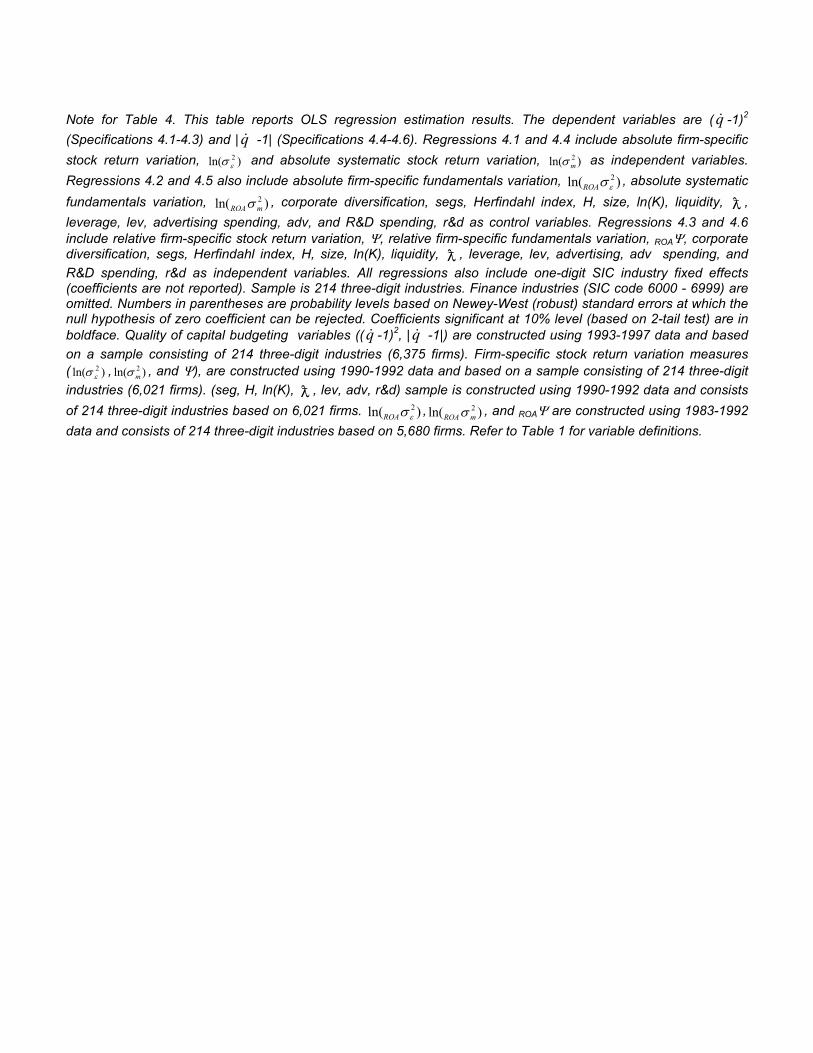
Note for Table 4. This table reports OLS regression estimation results. The dependent variables are ( &q -1)2 (Specifications 4.1-4.3) and | &q -1| (Specifications 4.4-4.6). Regressions 4.1 and 4.4 include absolute firm-specific stock return variation, )ln( 2
εσ and absolute systematic stock return variation, )ln( 2mσ as independent variables.
Regressions 4.2 and 4.5 also include absolute firm-specific fundamentals variation, )ln( 2εσROA , absolute systematic
fundamentals variation, )ln( 2mROAσ , corporate diversification, segs, Herfindahl index, H, size, ln(K), liquidity, D ,
leverage, lev, advertising spending, adv, and R&D spending, r&d as control variables. Regressions 4.3 and 4.6 include relative firm-specific stock return variation, Ψ, relative firm-specific fundamentals variation, ROAΨ, corporate diversification, segs, Herfindahl index, H, size, ln(K), liquidity, D , leverage, lev, advertising, adv spending, and R&D spending, r&d as independent variables. All regressions also include one-digit SIC industry fixed effects (coefficients are not reported). Sample is 214 three-digit industries. Finance industries (SIC code 6000 - 6999) are omitted. Numbers in parentheses are probability levels based on Newey-West (robust) standard errors at which the null hypothesis of zero coefficient can be rejected. Coefficients significant at 10% level (based on 2-tail test) are in boldface. Quality of capital budgeting variables (( &q -1)2, | &q -1|) are constructed using 1993-1997 data and based on a sample consisting of 214 three-digit industries (6,375 firms). Firm-specific stock return variation measures ( )ln( 2
εσ , )ln( 2mσ , and Ψ), are constructed using 1990-1992 data and based on a sample consisting of 214 three-digit
industries (6,021 firms). (seg, H, ln(K), D , lev, adv, r&d) sample is constructed using 1990-1992 data and consists of 214 three-digit industries based on 6,021 firms. )ln( 2
εσROA , )ln( 2mROAσ , and ROAΨ are constructed using 1983-1992
data and consists of 214 three-digit industries based on 5,680 firms. Refer to Table 1 for variable definitions.

Table 5 Nonlinear LS Regressions of the Capital Budgeting Quality Measures (Measured as Deviation from Threshold Value) on Firm-specific Stock
Return Variation and Control Variables 5.1 5.2 5.3 5.4 5.5 5.6
dependent variable
squared deviation of marginal q from an endogenously
estimated threshold value h, ( &q -h)2
absolute value of deviation of marginal q from an endogenously
estimated threshold value h, | &q -h|
0.757 0.754 0.753 0.808 0.786 0.719 threshold value of marginal q for capital
budgeting h (0.00) (0.00) (0.00) (0.00) (0.00) (0.00)
-0.185 -0.254 - -0.070 -0.081 - absolute firm-specific stock return variation )ln( 2
εσ (0.10) (0.05) (0.05) (0.05) 0.178 0.195 - 0.016 0.022 - absolute systematic stock
return variation )ln( 2mσ (0.15) (0.12) (0.50) (0.40)
- - -0.196 - - -0.028 relative firm-specific stock return variation Ψ
(0.08) (0.10) - 0.140 - - 0.051 - absolute firm-specific
fundamentals variation )ln( 2εσROA (0.19) (0.22)
- -0.061 - - -0.018 - absolute systematic fundamentals variation
)ln( 2mROAσ
(0.51) (0.68) - - 0.080 - - 0.031 relative firm-specific
fundamentals variation ROAΨ (0.38) (0.10) - 0.702 1.014 - -0.721 -0.490
corporate diversification segs (0.87) (0.81) (0.15) (0.20)
- -0.087 -0.080 - 0.494 0.588 Herfindahl index H (0.06) (0.08) (0.05) (0.01)
- 0.605 0.583 - 0.023 0.032 size ln(K) (0.33) (0.32) (0.10) (0.10)
- -0.295 -0.292 - -0.015 -0.010 liquidity D (0.07) (0.07) (0.81) (0.81)
- -0.164 -0.162 - -0.122 -0.128 leverage lev (0.37) (0.38) (0.05) (0.10)
- 3.294 3.353 - 1.666 1.113 advertising spending adv (0.04) (0.04) (0.30) (0.22)
- 1.870 1.886 - 0.974 0.968 R&D spending r&d (0.01) (0.01) (0.20) (0.18)
12.318 8.886 9.837 17.083 16.531 17.210 F-statistics
(0.00) (0.00) (0.00) (0.00) (0.00) (0.00) Regression R2 0.424 0.479 0.475 0.414 0.480 0.444
735.935 79.308 84.141 404.944 56.080 60.734 F-statistics of Wald test of comparison with
specification in Table 4 (0.00) (0.00) (0.00) (0.00) (0.00) (0.00)

Note for Table 5. This table reports non-linear LS regression estimation results. The dependent variables are ( &q - h)2 (Specifications 5.1-5.3) and | &q - h| (Specifications 5.4-5.6) where the threshold level h is estimated endogenously. Regressions 5.1 and 5.4 include absolute firm-specific stock return variation, )ln( 2
εσ and absolute systematic stock return variation, )ln( 2
mσ as independent variables. Regressions 5.2 and 5.5 also include absolute firm-specific fundamentals variation, )ln( 2
εσROA , absolute systematic fundamentals variation, )ln( 2mROAσ , corporate
diversification, segs, Herfindahl index, H, size, ln(K), liquidity, D , leverage, lev, advertising spending, adv, and R&D spending, r&d as control variables. Regressions 5.3 and 5.6 include relative firm-specific stock return variation, Ψ, relative firm-specific fundamentals variation, ROAΨ, corporate diversification, segs, Herfindahl index, H, size, ln(K), liquidity, D , leverage, lev, advertising, adv spending, and R&D spending, r&d as independent variables. All regressions also include one-digit SIC industry fixed effects (coefficients are not reported). Sample is 214 three-digit industries. Finance industries (SIC code 6000 - 6999) are omitted. Numbers in parentheses are probability levels based at which the null hypothesis of zero coefficient can be rejected. Coefficients significant at 10% level (based on 2-tail test) are in boldface. Wald test is computed for each specification in this table where a constraint regression is a corresponding regression in Table 5. Quality of capital budgeting variables (( &q -1)2, | &q -1|) are constructed using 1993-1997 data and based on a sample consisting of 214 three-digit industries (6,375 firms). Firm-specific stock return variation measures ( )ln( 2
εσ , )ln( 2mσ , and Ψ), are constructed using 1990-1992 data and
based on a sample consisting of 214 three-digit industries (6,021 firms). (seg, H, ln(K), D , lev, adv, r&d) sample is constructed using 1990-1992 data and consists of 214 three-digit industries based on 6,021 firms.
)ln( 2εσROA , )ln( 2
mROAσ , and ROAΨ are constructed using 1983-1992 data and consists of 214 three-digit industries based on 5,680 firms. Refer to Table 1 for variable definitions.

Figure 1
Stock Returns Synchronicity in Various Countries as Measured by the Average R2 of Regressions of Firm Returns on Domestic and US Market Returns
0% 5% 10% 15% 20% 25% 30% 35% 40% 45% 50% 55% 60%
United StatesIreland
CanadaU.K.
AustraliaNew Zealand
PortugalFrance
DenmarkAustriaHolland
GermanyNorway
IndonesiaSwedenFinland
BelgiumHong Kong
BrazilPhilippines
KoreaPakistan
ItalyCzech
IndiaSingapore
GreeceSpain
South AfricaColumbia
ChileJapan
ThailandPeru
MexicoTurkeyTaiwan
MalaysiaChina
Poland
Note for Figure 1. This figure presents Stock Returns Synchronicity in Various Countries as Measured by the Average R2 of Regressions of Firm Returns on Domestic and US Market Returns. See Yeung, Morck, Yu (2001).

Figure 2 The Deviation of Marginal Tobin’s q from One, with Industries Grouped by Industry-Average Firm-Level Market Model R2. A low R2 Indicates High Firm-specific Return Variation Relative to Market and Industry-related Variation. The Length of Each Bar Is the Group Average Deviation of Marginal q from One
0 0.25 0.5 0.75 1 1.25 1.5 1.75 2 2.25 2.5 2.75
0.00 to 0.05
0.05 to 0.10
0.10 to 0.15
0.15 to 0.20
0.20 to 0.25
0.25 to 0.30
0.30 to 0.35
0.35 to 0.40
0.40 to 0.45
0.45 to 0.50
above 0.5
Mar
ket M
odel
R-s
quar
ed S
tatis
tic
Deviation of Marginal q from 1
Squared Deviation of Marginal q from One Absolute Deviation of Marginal q from One

Figure 3
The Proportion of US Industry with Marginal Tobin’s q Significantly Greater or Lower Than One at a 10% Confidence Level, with Industries Grouped by Industry-Average Firm-Level Market Model R2. A low R2 Indicates a High Firm-specific Return Variation Relative to Market and Industry-related variation. The length of each bar is equal to the proportion of industries whose marginal q is significantly below or above 1 at 10% level
0% 10% 20% 30% 40% 50% 60% 70% 80% 90% 100%
0.00 to 0.05
0.05 to 0.10
0.10 to 0.15
0.15 to 0.20
0.20 to 0.25
0.25 to 0.30
0.30 to 0.35
0.35 to 0.40
0.40 to 0.45
0.45 to 0.50
above 0.50
Mar
ket M
odel
R-s
quar
ed S
tatis
tic
Fraction of Industries with Marginal q Significantly Different from One
fraction significantly below 1 fraction significantly above 1