value-at-risk and extreme returns - repub

Value-at-Riskand Extreme Returns

Jon DANIELSSON, Casper G. DE VRIES *

ABSTRACT. – We propose a semi-parametric method for unconditionalValue-at-Risk (VaR) evaluation. The largest risks are modelled parametri-cally, while smaller risks are captured by the non-parametric empirical dis-tribution function. A comparison of methods on a portfolio of stock andoption returns reveals that at the 5 % level the RiskMetrics analysis is best,but for predictions of low probability worst outcomes, it strongly underpre-dicts the VaR while the semi-parametric method is the most accurate.

Valeurs-à-Risque et les rendements extrêmes

RÉSUMÉ. – Nous présentons une méthode semi-paramétrique pourévaluer la valeur-à-risque (VaR). Les risques les plus grands sont modéli-sés paramétriquement, alors que les petits risques sont approchés par ladistribution empirique. Une comparaison des méthodes sur les rendementsd’un portefeuille d’actions et options montre qu’au niveau de confiance de5 %, la méthode proposée par J. P. MORGAN (RiskMetrics) est la meilleure,mais que pour les prédictions pour les plus grandes pertes à des basniveaux de probabilité, la méthode semi-paramétrique est supérieure, laméthode RiskMetrics sous-évalue la VaR.

* J. DANIELSSON: London School of Economics; C.G. DE VRIES: Tinbergen Institute andErasmus University Rotterdam.Our e-mail is [email protected] and [email protected] papers can be downladed from www.RiskResearch.org.We wish to thank F. X. DIEBOLD, P. HARTMANN, D. PYLE, T. VORST, E. ZIVOT, and workshopparticipants at the London School of Economics, University of Edinburgh, CambridgeUniversity, Pompeu Fabra University, Erasmus University Rotterdam and two refereesfor excellent comments. The University of Iceland research fund, the Fullbright program,and the Research Contribution of the Icelandic Banks supported this research. The firstdraft of this paper was written while the first author was visiting at the University ofPennsylvania, and we thank the university for its hospitality.

ANNALES D’ÉCONOMIE ET DE STATISTIQUE. – N° 60 – 2000

1 Introduction

A major concern for regulators and owners of financial institutions is catas-trophic market risk and the adequacy of capital to meet such risk. Wellpublicized losses incurred by several institutions such as Orange County,Procter and Gamble, and NatWest, through inappropriate derivatives pricingand management, as well as fraudulent cases such as Barings Bank, andSumitomo, have brought risk management and regulation of financial institu-tions to the forefront of policy making and public discussion.

A primary tool for financial risk assessment is the Value-at-Risk (VaR)methodology where VaR is defined as an amount lost on a portfolio with agiven small probability over a fixed number of days. The major challenge inimplementing VaR analysis is the specification of the probability distributionof extreme returns used in the calculation of the VaR estimate.

By its very nature, VaR estimation is highly dependent on good predictionsof uncommon events, or catastrophic risk, since the VaR is calculated fromthe lowest portfolio returns. As a result, any statistical method used for VaRestimation has to have the prediction of tail events as its primary goal.Statistical techniques and rules of thumb that have been proven useful inanalysis and prediction of intra-day and day-to-day risk, are not necessarilyappropriate for VaR analysis. This is discussed in a VaR context by e.g.DUFFIE and PAN [1997] and JORION [2000].

The development of techniques to evaluate and forecast the risk ofuncommon events has moved at a rapid rate, and specialized methods for VaRprediction are now available. These methods fall into two main classes: para-metric prediction of conditional volatilities, of which the J. P. MORGAN

RiskMetrics method is the best known, and non-parametric prediction ofunconditional volatilities such as techniques based on historical simulation orstress testing methods.

In this paper, we propose a semi-parametric method for VaR estimationwhich is a mixture of these two approaches, where we combine non-parame-tric historical simulation with parametric estimation of the tails of the returndistribution. These methods build upon recent research in extreme value-theory, which enable us to accurately estimate the tails of a distribution.DANIELSSON and DE VRIES [1997a] and DANIELSSON and DE VRIES [1997b]propose an efficient, semi-parametric method for estimating tails of financialreturns, and this method is expanded here to the efficient estimation of “port-folio tails”.

We evaluate various methods for VaR analysis, and compare the traditionalmethods with our tail distribution estimator using a portfolio of stocks. First,we construct a number of random portfolios over several time periods, andcompare the results of one step ahead VaR predictions. Second, we investi-gate multi-day VaR analysis. Third, we study the implications of adding anindex option to the portfolio. Fourth, the issues relating to the determinationof capital are discussed. Finally, we discuss the practical implementations ofthese methods for real portfolio management, with special emphasis on theease of implementation and computational issues.

240

2 The Methodologyof Risk Forecasting

2.1 Dependence

Financial return data are characterized by (at least) two stylized facts. First,returns are non-normal, with heavy tails. Second, returns exhibit dependencein the second moment. In risk forecasting, there is a choice between twogeneral approaches. The risk forecast may either be conditioned on currentmarket conditions, or can be based on the unconditional market risk. Bothapproaches have advantages and disadvantages, where the choice of methodo-logy is situation dependent.

2.1.1 Unconditional Models

A pension fund manager has an average horizon which is quite the oppositefrom an options trader. It is well known that conditional volatility is basicallyabsent from monthly return series, but the fat tail property does not fade. Forlonger horizon problems, an unconditional model is appropriate for the calcu-lation of large loss forecasts. Furthermore, even if the time horizon is shorter,financial institutions often prefer unconditional risk forecast methods to avoidundesirable frequent changes in risk limits for traders and portfolio managers.For more in this issue, see DANIELSSON [2000]. For a typical large portfolio(in terms of number of assets), the conditional approach may also just not befeasible since this requires constructing and updating huge conditionalvariance-covariance matrices.

2.1.2 Conditional Models

Building on the realization that returns exhibit volatility clusters, condi-tional volatility forecasts are important for several applications. In manysituations where the investment horizon is short, conditional volatility modelsmay be preferred for risk forecasting. This is especially the case in intra-dayrisk forecasting where predictable patterns in intra-day volatility seasonalityare an essential component of risk forecasting. In such situations bothGARCH and Stochastic Volatility models have been applied successfully. Ingeneral, where there are predictable regime changes, e.g. intra-day patterns,structural breaks, or macroeconomic announcements, a conditional model isessential. In the case of intra-day volatility, DANIELSSON and PAYNE [2000]demonstrate that traders in foreign exchange markets build expectations ofintra-day volatility patterns, where primarily unexpected volatility changesare important.

2.1.3 Conditionality versus Unconditionalityin Risk Forecasting

Neither the conditional nor the unconditional approach is able to tell whendisaster strikes, but GARCH type models typically perform worse when

VALUE-AT-RISK AND EXTREME RETURNS 241

disaster strikes since the unconditional approach structures the portfolioagainst disasters, whereas GARCH does this only once it recognizes one hashit a high volatility regime. Per contrast, GARCH performs better in signal-ling the continuation of a high risk regime since it adapts to the new situation.The conditional GARCH methodology thus necessarily implies more volatilerisk forecasts than the unconditional approach; see e.g. DANIELSSON [2000]who find that risk volatility from a GARCH model can be 4 times higher thanfor an unconditional model. Because the GARCH methodology quicklyadapts to recent market developments, it meets the VaR constraint morefrequently than the unconditional approach. But this frequency is just oneaspect, the size of the misses also counts. Lastly, conditional hedging can beself defeating at times it is most needed due to macro effects stalling themarket once many market participants receive sell signals from their condi-tional models, cf. the 1987 crash and the impact of portfolio insurance.

In the initial version of this paper, DANIELSSON and DE Vries [1997c],unconditional risk forecasts were recommended over the conditional type. Atthe time, empirical discussion of risk forecasting was in its infancy, and ourpurpose was primarily to introduce and demonstrate the uses of semi-parame-tric unconditional Extreme Value Theory (EVT) based methods. Thisapproach was subsequently criticized, in particular by MCNEIL and FREY

[1999], who propose a hybrid method, where a GARCH model is first esti-mated and EVT is applied to the estimated residuals. It is our present positionthat the choice of methodology should depend on the situation and question athand, and that both the conditional and unconditional approach belong in thetoolbox of the risk manager. In this paper, without prejudice, we focus onlyon the unconditional methods.

2.2 Data Features

In finance, it is natural to assume normality of returns in daily and multi-day conditional and unconditional volatility predictions, in applications suchas derivatives pricing. As the volatility smile effect demonstrates, however,for infrequent events the normal model is less useful. Since returns are knownto be fat tailed, the conditional normality assumption leads to a sizable under-prediction of tail events. Moreover, the return variances are well known tocome in clusters. The popular RiskMetrics technique, in essence an IGARCHmodel, is based on conditional normal analysis that recognizes the clusteringphenomenon and comes with frequent parameter updates to adapt to changingmarket regimes. The price one has to pay for the normality assumption andfrequent parameter updating is that such model is not well suited for analy-zing large risks. The normality assumption implies that one under estimatesthe chances of heavy losses. The frequent updating implies a high variabilityin the estimates and thus recurrent costly capital adjustments. For this reason,RiskMetrics focuses on the 5 % quantile, or the probability of losses thatoccur once every 20 days. These losses are so small that they can be handledby any financial institution. We argue below that RiskMetrics is ill suited forlower probability loses.

Furthermore, conditional parametric methods typically depend on condi-tional normality for the derivation of multi-period VaR estimates. Relaxation

242

of the normality assumption leads to difficulties due to the “square-root-of-time” method, i.e. the practice of obtaining multi-period volatility predictionsby multiplying the one day prediction by the square root of the length of thetime horizon. As CHRISTOFFERSEN and DIEBOLD [2000] argue, conditionalvolatility predictions are not very useful for multi-day predictions. We arguethat the appropriate method for scaling up a single day VaR to a multi-dayVaR is the alpha-root rule, where alpha is the number of finite boundedmoments, also known as the tail index. We implement the alpha-root methodand compare it with the square-root rule.

As an alternative to the fully parametric approach to (unconditional) VaRforecasts, one can either use the historical returns as a sampling distributionfor future returns as in Historical Simulation (HS) and stress testing, or use aform of kernel estimation to smooth the sampling distribution as in BUTLER

and SCHACHTER [1996]. The advantages of historical simulation have beenwell documented by e.g. JACKSON, MAUDE, and PERRAUDIN [1997], MAHONEY

[1996], and HENDRICKS [1996]. A disadvantage is that the low frequency andinaccuracy of tail returns leads to predictions which exhibit a very highvariance, i.e. the variance of the highest order statistics is very high, and is insome cases even infinite. As a result, the highest realizations lead to poor esti-mates of the tails, which may invalidate HS as a method for stress testing. Inaddition, it is not possible to do out-of-sample prediction with HS, i.e. predictlosses that occur less frequently than are covered by the HS sample period.

2.3 Properties of Extreme Returns

Value-at-Risk analysis is highly dependent on extreme returns or spikes.The empirical properties of the spikes, are not the same as the properties ofthe entire return process. A major result from empirical research of returns, isthe almost zero autocorrelation and significant positive serial correlation inthe volatility of returns. As a result volatilities can be relatively well predictedwith a parametric model such as ARCH. If, however, one focuses only onspikes, the dependency is much reduced. This is due to the fact that theARCH process is strong mixing (in combination with another technicalcondition). In DE HAAN, RESNICK, ROOTZEN, and DE VRIES [1989] it wasdemonstrated that the ARCH process satisfies these conditions so that if thethreshold level, indicating the beginning of the tails, rises as the sample sizeincreases, the spikes eventually behave like a Poisson process. In particular,for the ARCH(1) process DE HAAN, RESNICK, ROOTZEN, and DE VRIES [1989]obtain the tail index and the extremal index by which the mean cluster sizehas to be rescaled to obtain the associated independent process, see below.

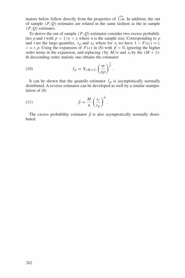
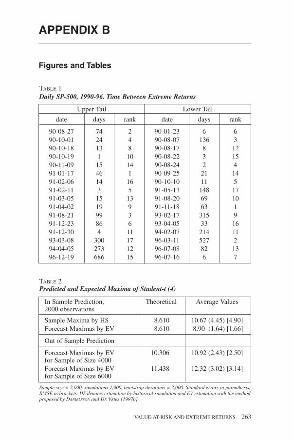
Some evidence for the reduced dependency over larger thresholds is givenin Table 1, which lists the number of trading days between the daily extremesfor the SP-500 index along with the rank of the corresponding observation.Figure 1 shows the 1 % highest and lowest returns on the daily SP-500 indexin the 1990’s along with the 7 stocks used below in testing the VaR estimationtechniques. No clear pattern emerges for these return series. In some cases wesee clustering, but typically the extreme events are almost randomly scattered.Furthermore, there does not appear to be strong correlation in the tail events.


There were 2 days when 5 assets had tail events, no days with 4 tail events, 5 days with 3 events, 21 days with 2 events, 185 days with 1 event, and 1,558days with no tail events. For the SP-500, two of the upper tail observationsare on adjacent days but none of the lower tailed observations, and in mostcases there are a number of days between the extreme observations. One doesnot observe market crashes many days in a row. There are indications of someclustering of the tail events over time. However, the measurement of a spikeon a given day, is not indicative of a high probability of a spike the followingfew days. The modelling of the dependency structure of spikes would there-fore be different than in e.g. GARCH models.

Another important issue is pointed out by DIMSON and MARSH [1996] whoanalyze spikes in 20 years of the British FTSE All Share Index, where theydefine spikes as fluctuations of 5 % or more. They find 6 daily spikes,however they also search for non-overlapping multi day spikes, and find 4 2-day spikes, 3 3-day, 3 4-day, 8 weekly, and up to 7 biweekly. Apparently, thenumber of spikes is insensitive to the time span over which the returns aredefined. This is an example of the fractal property of the distribution ofreturns and the extremes in particular, and is highly relevant for spike forecas-ting when the time horizon is longer than one day.

On the basis of the above evidence, we conclude that for computing theVaR, which is necessarily concerned with the most extreme returns, theARCH dependency effect is of no great importance. One can show, moreover,that the estimators are still asymptotically normal, albeit with higher variancedue to the ARCH effect. Hence, it suffices to assume that the highest andlowest realizations are i.i.d. This is corroborated by the evidence fromCHRISTOFFERSEN and DIEBOLD [2000] that when the forecast horizon is severaldays, conditional prediction performs no better than using the unconditionaldistribution as predictive distribution. The reason is that most current historycontains little information on the likelihood that a spike will occur, especiallyin the exponential weighting of recent history by RiskMetrics.

3 Modelling Extremes

3.1 Tail Estimation

Extreme value theory is the study of the tails of distributions. Severalresearchers have proposed empirical methods for estimation of tail thickness.The primary difficulty in estimating the tails is the determination of the startof the tails. Typically, these estimators use the highest/lowest realizations toestimate the parameter of tail thickness which is called the tail index. HILL

[1975] proposed a moments based estimator for the tail index. The estimatoris conditional on knowing how many extreme order statistics for a givensample size have to be taken into account. HALL [1990] suggested a bootstrapprocedure for estimation of the start of the tail. His method is too restrictive tobe of use for financial data, e.g., it is not applicable to the Student-t distribu-

244

tion, which has been used repeatedly to model asset returns. Recently,DANIELSSON and DE VRIES [1997a] and DANIELSSON, DE HAAN, PENG, DE

VRIES [2000] have proposed general estimation methods for the number ofextreme order statistics that are in the tails, but presuppose i.i.d. data.1 Thismethod is used here to choose the optimal number of extreme order statistics.A brief formal summary of these results is presented in Appendix A.

It is known that only one limit law governs the tail behavior of data drawnfrom almost any fat tailed distribution.2 The condition on the distributionF(x) for it to be in the domain of attraction of the limit law is given by (7) inAppendix A. Since financial returns are heavy tailed, this implies that forobtaining the tail behavior we only have to deal with this limit distribution.By taking an expansion of F(x) at infinity and imposing mild regularityconditions one can show that for most heavy tailed distributions the secondorder expansion of the tails is:

(1) F(x) � 1 − ax−α[1 + bx−β

], α,β > 0

for x large, while a, b, α, and β are parameters. In this expansion, the keycoefficient is α, which is denoted as the tail index, and indicates the thicknessof the tails. The parameter a determines the scale, and embodies the depen-dency effect through the extremal index; the other two parameters b and β arethe second order equivalents to a and α. For example, for the Student-t or thenon-normal stable densities, α equals the degrees of freedom or the characte-ristic exponent. For the ARCH process α equals the number of boundedmoments of the unconditional distribution of the ARCH innovations.

HILL [1975] proposed a moments based estimator of the tail index which isestimated conditional on a threshold index M where all values xi > X M+1are used in the estimation. The Xi indicate the decreasing order statistics,X1 � X2 � ... � X M � ... � Xn, in a sample of returns x. DANIELSSON andDE VRIES [1997] discuss the following estimator for the tail probabilities,given estimates of α and the threshold:

(2) F̂(x) = p = M

n

(X M+1

x

)α̂

, x > X M+1

where n is the number of observations, and p is the probability. This appliesequally to the lower tails. By taking the inverse of F̂(x) we obtain an extremequantile estimator:

(3) x̂p = F̂−1(x) = X M+1

(M

np

) 1α̂

.

Note that F̂(x) is always conditional on a given sample. In order to use thedistribution F̂(x) we need to specify the parameters α and the randomvariables M and X M+1, before we can obtain a quantile estimate for a proba-bility. The empirical and estimated distribution functions of the SP-500 index


1. For dependent data it is not known yet how to choose the number of highest order statistics opti-mally.

2. DANIELSSON and DE VRIES [1997a] discuss this issue in details some.

are presented in Figure 3. Some practical issues of the tail estimation arediscussed below.

3.2 Multi-Period Extreme Analysis

The method for obtaining multi-period predictions follows from the work ofFELLER [1971, VIII.8]. FELLER shows that the tail risk for fat tailed distribu-tions is, to a first approximation, linearly additive. Assume that the tails of thedistribution are symmetric in the sense that for a single period returnPr [|X | > x] ≈ ax−α when x is large.3 For the T-period return we then have

(4) Pr [X1 + X2 + ... + Xn > x] ≈ T ax−α.

The implication for portfolio analysis of this result has been discussed inthe specific case of non-normal stable distributions by FAMA and MILLER

[1972, p. 270]. In that case α < 2 and the variance is infinite. DACOROGNA,MULLER, PICTET, and DE VRIES [1995] are the first to discuss the finitevariance case when α > 2. It is well known that the self-additivity of normaldistributions implies that the T 1/2 scaling factor for multi-period VaR, i.e. the“square-root-of-time rule” implemented in RiskMetrics. But for heavy taileddistributions this factor is different for the largest risks. Heavy tailed distribu-tions are self-additive in the tails, see e.g. (4). This implies a scaling factorT 1/α for VaR in a T-period analysis. With finite variance where α > 2 andhence T 1/2 > T 1/α, i.e. the scaling factor for heavy tailed distributed returnsis smaller than for normal distributed returns. In comparison with the normalmodel, there are two counter balancing forces. If daily returns are fat taileddistributed, then there is a higher probability of extreme losses and thisincreases the one day possible loss vis-à-vis the normal model. This is a leveleffect. But there is also a slope effect. Due to the above result, the multiplica-tion factor (slope) used to obtain the multi-day extreme is smaller for fattailed distributed returns than for normal returns. For this reason, extremepredictions from the two models cross at different probability levels if weconsider different time horizons. This is demonstrated in Table 5.

3.3 Monte Carlo Evidence

In order to evaluate the performance of the estimated tail distribution in (2)DANIELSSON and DE VRIES [1997a] do extensive Monte Carlo experiments toevaluate the properties of the estimator. In Table 2, a small subset of theresults is presented. We generate repeated samples of size 2000 from aStudent-t distribution with 4 degrees of freedom and compare the averagemaxima, denoted here as the sample maxima by historical simulation (HS),from the samples with the average predicted value by F̂(x), denoted asextreme value (EV). The specific distribution was chosen since its tail beha-vior is similar to a typical return series. The Monte Carlo results are reportedin Table 2.

246

3. For more general results and conditions on the tails, see GELUK, PENG, DE VRIES [2000].

Out-of-sample predictions were obtained by using the estimated tail of thedistribution to predict the value of the maxima of a sample of size 4,000 and6,000, the true values are reported as well. We can see that the tail estimatorperforms quite well in predicting the maxima while the sample averages yieldmuch lower quality results. Note that the variance of HS approach is muchhigher than the variance by EV method. Moreover, HS is necessarily silent onthe out of sample sizes 4,000 to 6,000, where EV provides an accurate esti-mate. Obviously, if one used the normal to predict the maximums, the resultwould be grossly inaccurate, and would in fact predict values about one thirdof the theoretical values. See also Figures 3 and 4 in Section 5 below for agraphical illustration of this claim.

4 Value-at-Riskand Common Methods

Value-at-Risk form the basis of the determination of market risk capital (seeSection 6.1.3). The formal definition of Value-at-Risk (VaR) is easily givenimplicitly:

(5) Pr [�P�t � V a R] = π,

where �P�t is a change in the market value of portfolio P over time horizon�t with probability π. Equation (5) states that a loss equal to, or larger thanthe specific VaR occurs with probability π. Or conversely, (5) for a givenprobability π losses, equal to or larger than the VaR, happen. In this latterinterpretation the VaR is written as a function of the probability π. LetF(�P�t ) be the probability distribution of �P�t, then

(6) F−1(π) = V a R;where F−1(·) denotes the inverse of F(·). The major problem in implemen-ting VaR analysis is the specification of the probability distribution F(·)which is used in the calculation in (5).

Two methods are commonly used to evaluate VaR:

1. Historical Simulation (Non Parametric, Unconditional Volatility)2. Parametric Methods (Fully Parametric, Conditional Volatility)

Both these methods are discussed in this section. The semi-parametricextreme value (EV) method falls in between these two methodologies.

4.1 Historical Simulation

A popular method for VaR assessment is historical simulation (HS). Insteadof making distributional assumptions about returns, past returns are used topredict future returns.


The advantage of historical simulation is that few assumptions are required,and the method is easy to implement. The primary assumption is that thedistribution of the returns in the portfolio is constant over the sample period.Historical simulation has been shown to compare well with other methods,see e.g. MAHONEY [1996], however past extreme returns can be a poorpredictor of extreme events, and as a result historical simulation should beused with care. The reason for this is easy to see. By its very nature HS hasnothing to say about the probability outcomes which are worse than thesample minimum return. But HS also does not give very accurate probabilityestimates for the borderline in sample extremes, as is demonstrated below.Furthermore, the choice of sample size can have a large impact on the valuepredicted by historical simulation. In addition, the very simplicity of HSmakes it difficult to conduct sensitivity experiments, where a VaR isevaluated under a number of scenarios.

A major problem with HS is the discreteness of extreme returns. In theinterior, the empirical sampling distribution is very dense, with adjacentobservations very close to each other. As a result the sampling distribution isvery smooth in the interior and is the mean squared error consistent estimateof the true distribution. The closer one gets to the extremes, the longer theinterval between adjacent returns becomes. This can be seen in Table 3 wherethe 7 largest and smallest returns on the stocks in the sample portfolio andSP-500 Index for 10 years are listed.

These extreme observations are typically the most important for VaRanalysis, however since these values are clearly discrete, the VaR will also bediscrete, and hence be either underpredicted or overpredicted. We see that thiseffect is somewhat more pronounced for the individual assets, than for themarket portfolio SP-500, due to diversification. Furthermore, the variance ofthe extreme order statistics is very high; and can be infinite. As a result, VaRestimates that are dependent on the tails, will be measured discretely, with ahigh variance, making HS in many cases a poor predictor of the VaR. Resultsfrom a small Monte Carlo (MC) experiment demonstrating this are presentedin Section 3.3. In Figure (2) we plot the 99th percentile of the S&P for thepast 500 and 1,000 days, i.e. the 5th and 10th largest and smallest observationsfor the past 500 and 1,000 days respectively. It is clear from the figure that thewindow length in assessing the probability of spikes is very important, andthis creates a serious problem. Note how rapidly the percentile changes whennew data enter and exit the window. In VaR prediction with HS, the inclusionor exclusion of one or two days at the beginning of the sample can cause largeswings in the VaR estimate, while no guidelines exist for assessing whichestimate is the better.

BUTLER and SCHACHTER [1996] propose a variation of HS by use of a kernelsmoother to estimate the distribution of returns, which is in essence an esti-mation of the distribution of returns. This type of methodology has bothadvantages and draw backs. The advantage is that a properly constructedkernel distribution provides a smooth sampling distribution. Hence sensitivityexperiments can be readily constructed, and valuable insight can be gainedabout the return process. Furthermore, such distribution may not be as sensi-tive to the sample length as HS is. Note that these advantages are dependenton a properly constructed kernel distribution. In kernel estimation, thespecific choice of a kernel and window length is extremely important. Almost

248

all kernels are estimated with the entire data set, with interior observationsdominating the kernel estimation. While even the most careful kernel estima-tion will provide good estimates for the interior, there is no reason to believethat the kernel will describe the tails adequately. Tail bumpiness is a commonproblem in kernel estimation. Note especially that financial data are thicktailed with high excess kurtosis. Therefore, a Gaussian kernel, which assumesthat the estimated distribution has the same shape as the normal, is unsuitablefor financial data.

A referee suggested that an optimal window length might be obtained fromeconomic rather than statistical considerations. This is an appropriate recom-mendation for those who plan to apply kernel estimation to risk problems. Inaddition, we feel that a similar suggestion could also apply to the choice ofnumber of extreme order statistics in EVT estimation, specifically that amoney metric may be an appropriate side constraint; cf. PENG [1998].

4.2 Parametric Forecasting

In parametric forecasting, the predicted future volatility of an asset is anexplicit function of past returns, and the estimated model parameters. Themost common models are the unconditional normal with frequently updatedvariance estimate, or explicit models for conditional heteroscedasticity likethe GARCH model, with normal innovations. The popular RiskMetricsapproach which uses the frequently updated normal model is asymptoticallyequivalent to an IGARCH model. This implies a counterfactual hypothesis ofan unconditional infinite variance. However, since in most cases, only shorthorizon conditional forecasts are made, this does not affect the results signifi-cantly. GARCH models with normal innovations have proved valuable inforecasting common volatilities, however they perform poorly in predictingextreme observations, or spikes, in returns. Furthermore, while the GARCHnormal model unconditionally has heavy tails, conditionally, they are thin.The normality assumption is primarily a matter of convenience, and aGARCH model with non-normal innovations can easily be estimated, withthe most common specification being the Student-t. The advantage ofStudent-t innovations is that they are thick tailed and hence will in generalprovide better predictive densities; note that the Student-t contains Gaussianerrors as a special case. The disadvantages of non-normal innovations for theVaR exercise are several, e.g. multivariate versions of such models are typi-cally hard to estimate and recursive forecasts of multi-step ahead VaR levelsare difficult to compute, since the GARCH process is not self additive.

There are several reasons for the failure of RiskMetrics to adequatelycapture the tail probabilities. For example, the normal likelihood functionweight values close to zero higher than large values, so the contribution of thelarge values to the likelihood function is relatively small. Since most observa-tions are in the interior, they dominate the estimation, especially since tailevents are may be 1-2 % of the observations. While a GARCH model withnormal innovations preforms poorly, it does not imply that parametric fore-casting will in general provide biased VaR estimates, however such a modelwould have to be constructed with the tails as the primary focus. SeeJACKSON, MAUDE, and PERRAUDIN [1997] for discussion on this issue.


There is yet another problem with the way RiskMetrics implements theGARCH methodology. Instead of going by the GARCH scheme for predictingfuture volatilities, RiskMetrics ignores GARCH and simply uses the square-root-of-time method which is only appropriate under an i.i.d. normal assumption. Ifthe predicted next day volatility is σ̂ 2

t+1, then the predicted T day ahead volatilityis T σ̂ 2

t+1 in the RiskMetrics analysis. This implies that for the next T days,returns are essentially assumed to be normally distributed with variance T σ̂ 2

t+1.The underlying assumption is that returns are i.i.d., in which case there would beno reason to estimate a conditional volatility model. Note that this problem canbe by passed by using T day data to obtain T day ahead predictions as suggestedin the RiskMetrics manual. But the methodology of entertaining differentGARCH processes at different frequencies lacks internal consistency.

In Table 4, we show the six highest and lowest returns on the daily SP-500index from 1990 to 1996, or 1,771 observations. We used the normal GARCHand Student-t GARCH models to predict the conditional volatility, and show,in the table, the probability of an outcome equal to or more extreme than theobserved return, conditional on the predicted volatility for each observation.In addition, we show the probability as predicted by the extreme value esti-mator, and values of the empirical distribution function. We see from the tablethat the normal GARCH model performs very poorly in predicting tail events,while the Student-t GARCH model gives some what better results. Bothmethods are plagued by high variability and inaccurate probability estimates,while the extreme value estimator provides much better estimates.

5 Extreme Value Theory and VaR

Accurate prediction of extreme realizations is of central importance to VaRanalysis. VaR estimates are calculated from the lower extreme of a portfolioforecast distribution; therefore, accurate estimation of the lower tail of port-folio returns is of primary importance in any VaR application. Most availabletools, such as GARCH, are however designed to predict common volatilities,and therefore have poor tail properties. Even historical simulation (HS) hasless than desirable sampling properties out in the tails. Therefore, a hybridtechnique that combines sampling from the empirical distribution for commonobservations with sampling from a fitted tail distribution has the potential toperform better than either HS or fully parametric methods by themselves.

In Figure 3, the empirical distribution of the SP-500 index is plotted alongwith the fitted power tail distribution F(x) and the estimated normal distribu-tion. We see the problems with HS in the tails from Figure 3, e.g. discretenessof observations and the inability to provide out-of-sample low probabilitypredictions. The normal distribution clearly under estimates the probability ofthe highest returns. On the other hand, the fitted distribution is a smooth func-tion through the empirical distribution, both in and out of sample. Forcomparison, in figure 4 we plot the fitted distribution along with the normaldistribution estimated from the sample mean and variance, and the distribu-

250

tion obtained from the normal GARCH(1,1) process if one conditions on themaximum observed past volatility. This means that the normal distribution,with the variance of the largest of the one day GARCH volatility predictions,is plotted. This gives the normal GARCH the maximum benefit of the doubt.Since this conditional distribution is still normal, it underestimates theextreme tails. There are several advantages in using the estimated power tailin VaR estimation. For example:

• In HS, the presence of an event like the ‘87 crash in the sample,will causea large VaR estimate. However, since a ‘87 magnitude crash only occursrarely, say once every 60 years, the presence of such an event in thesample will produce upward biased VaR estimates. And, hence, imposestoo conservative capital provisions. By sampling from the tail distribu-tion, the probability of a ‘87 type event will be much smaller, leading tobetter VaR estimates.

• The empirical distribution is sampled discretely out in the tails, with thevariance of the extreme order statistics being very high. This implies thata VaR that relies on tail realizations will exhibit the same properties, withthe resulting estimates being highly variable. A Monte Carlo example ofthis is given in Table 2.

• By sampling from the tail of the distribution, one can easily obtain thelowest return that occurs at a given desired probability level, say 0.1 %,greatly facilitating sensitivity experiments. This is typically not possiblewith HS by itself.

• The probability theory of tail observations, or extreme value theory, is wellknown, and the tail estimator therefore rests on firm statistical foundations.In contrast, most traditional kernel estimators have bad properties in the tails.

5.1 Estimated Tails and Historical Simulation

We propose combining the HS for the interior with the fitted distribution from(1) along the lines of DANIELSSON and DE VRIES [1997a]. Recall from above thatthe fitted distribution, F̂(x), is conditional on one of the highest order statisticsX M+1. Therefore, we can view X M+1 as the start of the tail, and use F̂(x) asthe sampling distribution for extreme returns. Below this threshold X M+1 wecan see the empirical distribution for interior returns. This can be implementedin the following algorithm, where X Mupper+1 and X M lower−1 are the thresholdsfor the upper and lower tail respectively, and T is the window size.

Draw xs from {xt }Tt=1 with replacement

if xs < X M lower−1 thendraw xs from F̂(x) for the lower tail

elseif xs > X Mupper+1then

draw xs from F̂(x) for the uper tailelse

keep xs

end ifend if


Note that this guarantees that the combined density integrates out to one.Wecan then view x as one draw from the combined empirical and extreme valuedistributions, and we denote the method as the combined extreme value esti-mator and historical simulation method.

5.2 Tails of Portfolios

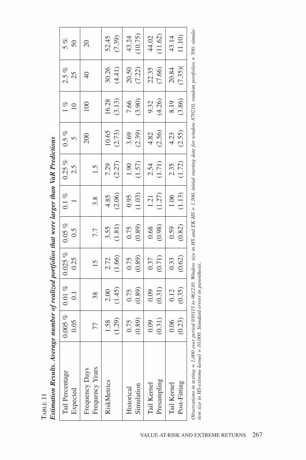
In general, multiple assets are used to construct a portfolio. We can imple-ment simulations of portfolio returns with one of two methods, post fitting orpre-sampling. Results from implementing both methods are presented inTable 11 and discussed below. Note that while we would not necessarilyexpect strong interdependency between the tails of stock returns, strong tail“correlation” is often expected in exchange rates, e.g. in the EMS, largemovements often occur at the same time for several countries.

5.2.1 Post-Fitting

In post-fitting, one proceeds along the lines of the combined extreme valueand historical simulation procedures and applies the current portfolio weightsto the historical prices to obtain a vector of simulated portfolio returns. This isexactly as in historical simulation. Subsequently, the tails of the simulatedreturns are fitted, and any probability-VaR combination can be read from thefitted tails. This procedure has several advantages. No restrictive assumptionsare needed, the method can be applied to the largest of portfolios, and doesnot require significant additional computation time over HS. The primarydisadvantage is that it carries with it the assumption of constant correlationacross returns, while systematic changes in correlation may occur over time.However, in the results below this does not seem to cause any significantproblems.

5.2.2 Presampling

In the presampling method, each asset is sampled independently from thehybrid extreme value estimator and empirical distribution, and subsequentlyscaled to obtain properly correlated returns. Then the value of the portfolio iscalculated. The scaling is achieved as follows. Let �t be the covariance matrixof the sample, and Lt L ′

t = �t be the Cholesky transformation. The number ofassets in the portfolio is K and the number of simulations is N. We then draw aK N matrix of simulated returns, denoted as X̃n. Let the covariance matrix ofX̃n be denoted by �n, with the Cholesky transformation Mn M ′

n = �n. ScaleX̃n to an identity covariance matrix by M−1

n X̃n, which can then be scaled tothe sample covariance by Lt. The matrix of simulated returns X is:

Xn = Lt M−1n X̃n.

If w = {wi }Ki=1 is the vector of portfolio weights, the simulated return

vector R is:

Rn =K∑

i=1

wi Xt,n,i n = 1,N .

252

By sorting the simulated portfolio returns R, one can read off the tail proba-bilities for the VaR, in the same manner as in HS. By using this method, it ispossible to use a different covariance matrix for sub samples than for thewhole sample. This may be desirable when the covariance matrix of returnschanges over time where it may yield better results to replace the covariancematrix � with the covariance matrix of the last part of the sample. If theeffects of a regime change can be anticipated by imputing the appropriatechanges in the covariance structure, such as in the case of monetary unifica-tion, the presampling approach has an advantage over the post-fitting method.

6 Estimation

To test the performance of our VaR procedure, we selected 6 US stocksrandomly as the basis for portfolio analysis in addition to the JP Morgan bankstock price. The stocks in the tables are referred by their ticker tape symbols.The window length for HS and the combined extreme value-empirical distri-bution procedure was set at 6 years or 1,500 trading days. Note this is muchlarger than the regulatory window length of one year. The reason for this longperiod is that for accurate estimation of events that happen once every100 days, as in the 1 % VaR, one year is not enough for accurate estimation.In general, one should try to use as large a sample as is possible. Using asmaller sample than 1,500 trading days in the performance testing was notshown to improve the results. Performance testing starts at Jan. 15. 1993, andthe beginning of the sample is 1,500 days before that on Feb. 12, 1987. It is astylized fact in empirical studies of financial returns, that returns exhibitseveral common properties, regardless of the underlying asset. This extends tothe tails of returns. In Table 12, we present summary statistics on a widerange of financial returns for the period 1987-1996, and it is clear that thetails all have similar properties. Summary statistics for each stock return arelisted in Table 7 for the entire sample period, and in Table 8 for the 1990-1996testing period. The corresponding correlation matrixes are presented inTables 9 and 10. The sample correlations drop in the 1990’s. Given thischange in correlation, we tested changing correlations in the pre-fittingmethod, but it did not have much impact for our data, and therefore we do notreport those results here.

6.1 VaR Prediction

6.1.1 Interpretation of Results

Results are reported in Table 11. The VaR return estimates for each methodare compared with the realized returns each day. The number of violations ofthe VaR estimates were counted, and the ratio of violations to the length of thetesting period was compared with the critical value. This is done for severalcritical values. This is perhaps the simplest possible testing procedure. Several


authors, most recently DAVÉ and STAHL [1997], propose much more elaboratetesting procedures, e.g. the likelihood based method of DAVÉ and STAHL whichis used to test a single portfolio. However by using a large number of randomportfolios one obtains accurate measurements of the performance of thevarious methods, without resorting to specific distributional assumptions, suchas the normality assumption of DAVÉ and STAHL. In addition, while the green,yellow, and red zone classification method proposed by BIS may seem attrac-tive for the comparison, it is less informative than the ratio method used here.

The test sample length was 1,000 trading days, and the window size in HS andEV was 1,500. For the 1 % risk level, we expect a single violation of the VaRevery 100 days, or 10 times over the entire testing period. This risk level is givenin the eight column from the left in Table 11. At this risk level RiskMetrics yieldstoo many violations, i.e. 16.3, on average, while the other methods give too fewviolations, or from 7.6 for HS to 9.3 for the presampling EV method, on average.If the number of violations is higher than the expected value, it indicates that thetails are underpredicted, thinner or lower than expected, and conversely too fewviolations indicate that the estimated tail is thicker than expected. In addition tothe tail percentages, we show the implied number of days, i.e. how frequentlyone would expect a tail event to occur. If the number of days is large, we trans-form the days into years, assuming 260 trading days per year.

6.1.2 Comparison of Methods

For the 5th percentile, RiskMetrics performs best. The reason for this is thatat the 5 % level we are sufficiently inside the sample so that the conditionalprediction performs better than unconditional prediction. However, as wemove to the tails, RiskMetrics consistently underpredicts the tail, with everlarger biases as we move farther into the tails. For example, at the 0.1 % levelRiskMetrics predicts 5 violations, while the expected number is one.Therefore RiskMetrics will underpredict the true number of losses at a givenrisk level. Historical simulation has in a way the opposite problem, in that itconsistently overpredicts the tails. Note that for HS we can not obtain esti-mates for lower probabilities than one over the sample size, or in our caseprobabilities lower than once every 1,500 days. Hence the lowest prediction,0.75, is repeated in the last four columns in the table. Obviously for smallersample sizes HS is not able to predict the VaR for even relatively high proba-bilities. Both EV estimators have good performance, especially out in thetails. The presampling version of the EV estimator can not provide estimatesfor the lowest probability. The simulation size was 10,000 and this limits thelowest probability at 1/10,000. The post fitting version has no such problems.It is interesting to note that the EV estimators do a very good job at trackingthe expected value of exceedances. Even at the lowest probability, theexpected value is 0.05 while the post fitting EV method predicts 0.06.

6.1.3 Implication for Capital Requirements

A major reason for the implementation of VaR methods is the determinationof capital requirements (CR). Financial regulators determine the CR accor-ding to the formula

CR = 3 × VaR + constant

254

Individual financial institutions estimate the VaR, from which the CR arecalculated. If the banks underestimate the VaR they get penalized by anincrease in the multiplicative factor or the additive constant. The multiplica-tive constant may be increased to 4. If, however, the financial institution overestimates the VaR, it presumably gets penalized by shareholders. Hence accu-rate estimation of the VaR is important. The scaling factor 3 appears to besomewhat arbitrary, and has come under criticism from financial institutionsfor being too high. STAHL [1997] argues that the factor is justified by applyingChebyshev’s inequality to the ratio of the true and model VaR distributions. Inthis worst case scenario, STAHL calculates 2.7 as an appropriate scaling factorat the 5 % level, 4.3 at the 1 % level, and increasing with lower probabilities.But according to Table 11, this factor is much too high or conservative. Bycomparing the RiskMetrics and the EV results at the 5 % level, we see thatthey are very close to the expected number of violations, and in that case amultiplicative constant close to one would be appropriate. At the 0.1 % level,RiskMetrics has five times the expected number of violations and in that casea large multiplicative constant may be appropriate, but the EV method givesresults close to the expected value, suggesting that the constant should beclose to one if EV is used for VaR. While a high scaling factor may be justi-fied in the normal case, by using the estimate of the tails, as we do with theEV method, the multiplicative factor can be taken much lower. Note that HS,implies too high capital requirements in our case, while RiskMetrics impliestoo low CR. The extreme value estimator method appears to provide accuratetail estimates, and hence the most accurate way to set capital requirements.4

DANIELSSON, HARTMANN, and DE VRIES [1998] raise an issue regardingimplications for incentive compatibility. The banks want to keep capitalrequirements as low as possible, and are faced with a sliding multiplicativefactor in the range from three to four. Given that using a simple normal modelimplies considerably smaller capital requirements than the more accuratehistorical simulation or extreme tail methods, or even RiskMetrics, and thatthe penalty for under predicting the VaR is relatively small, i.e. the possibleincrease from 3 to 4, it is in the banks best interest to use the VaR methodwhich provides the lowest VaR predictions. This will, in general be close tothe worst VaR method available. This may explain the current prevalenceamong banks of using a moving average normal model for VaR prediction. Itis like using a protective sunblock, because one has to, but choosing the onewith lowest protection factor because its cheapest, with the result that one stillgets burned.

6.2 Multi-Day Prediction

While most financial firms use one day VaR analysis for internal riskassessment, regulators require VaR estimates for 10 day returns. There aretwo ways to implement a multi-day VaR. If the time horizon is denoted by T,one can either look at past non-overlapping T day returns, and use these in thesame fashion as the one day VaR analysis, or extrapolate the one day VaR


4. For more general results and conditions on the tails, see GELUK, PENG, DE VRIES [2000].

returns to the T day VaR. The latter method has the advantage that the samplesize remains as it is. Possibly for this reason, RiskMetrics implements thelatter method by the so called “square-root-of-time” rule which implies thatreturns are normal with no serial correlation. However, for fat tailed data, aT 1/α is appropriate. See section 3.1 for discussion on this issue.

It is not possible to backtest the T = 10 day VaR estimates because wehave to compare the VaR predictions with non-overlapping T day returns.This implies that the sample available for testing is T times smaller than theone day sample. Since we are looking at uncommon events, we need to back-test over a large number of observations. In our experience, 1,000 days is aminimum test length. Therefore, for 10 day VaR we would need 10,000 daysin the test sample.

In order to demonstrate the multi-day VaR methods, we use the one dayVaR at the last day of our sample, December 30, 1996 to obtain 10 day VaRs.This is the VaR prediction on the last day of the results in Table 1, the numberof random portfolios was 500. In Table 5, we present the one day and 10 dayVaR predictions from RiskMetrics type and extreme value post-fittingmethods. The numbers in the table reflect losses in millions of dollars on aportfolio of 100 million dollars. We see in Table 5 the same result as inTable 11, i.e. RiskMetrics underpredicts the amount of losses vis-à-vis EV atthe 0.05 % and 0.005 % probabilities, while for the 10 day predictionsRiskMetrics over predicts the loss, relative to EV, even for very low risklevels. Recall that EV uses the multiplicative factor T 1/α while RiskMetricsuses T 1/2. Due to this, the loss levels of the two methods cross at differentprobability levels depending on the time horizon. The average α was 4.6, withthe average scaling factor of 1.7 which is much smaller than T 1/2 = 3. 7. Asa result, at the 0.05 % level RiskMetrics predicts a 10 day VaR of $6.3mwhile EV only predicts $5.1m, on average.

6.3 Options

The inclusion of liquid nonlinear derivatives like options in the portfoliodoes not cause much extra difficulty. In general one has to price the option bymeans of risk neutral probabilities. However, the risk neutral measure is notobserved, at least not directly. This is a generic problem for any VaR method,and for this reason RiskMetrics proceeds under the assumption of risk neutra-lity, and the assumption is followed here as well. The extreme value methodcan be used to generate the data for the underlying asset, and these simulateddata can be used to price the option under risk neutrality. A structured MonteCarlo method is easily implemented by the post fitting method.

For simulation of returns on an European option, the path of returns on theunderlying is simulated from the current day until expiration, sampling eachday return from the combined empirical and estimated distributions, asdescribed above, with the mean subtracted, and summing up the one dayreturns to obtain a simulated return for the entire period, yi. If P F is thefuture spot price of the asset, then a simulated future price of the underlying isP F exp [yi ], and the simulated payoff follows directly. By repeating this Ntimes, we get a vector of simulated options payoffs, which is discounted backwith the rescaled three month t-bill rate, the vector is averaged, and the price

256

of the option is subtracted. We then update the current futures price by oneday through an element from the historical return distribution of the under-lying, and repeat the simulation. This is done for each realization in thehistorical sample. Together this gives us the value of the option, and a vectorof option prices quoted tomorrow. Finally, we calculate the one day optionreturns and can treat these returns as any other asset in the portfolio.

We used the same data as in the VaR exercise above, and added a Europeanput option on the SP-500 index to the portfolio. The VaR was evaluated withvalues on September 4, 1997, the future price of the index was 943 and thestrike price was 950. We used random portfolio weights, where the optionreceived a weight of 4.9 %, and evaluated the VaR on the portfolio with andwithout the option. The results are in Table 6, where we can see that the optionresults in lower VaR estimates than if it is left out. Interestingly, the differencesin monetary value are the greatest at the two confidence levels in the middle.

7 Practical Issues

There are several practical issues in implementing the extreme valuemethod, e.g. the length of the data set, the estimation of the tail shape, and thecalculation of the VaR for individual portfolios.

For any application where we are concerned with extreme outcomes, orevents that happen perhaps once every 100 days or less, as is typical in VaRanalysis, the data set has to include a sufficient number of extreme events inorder to obtain an accurate prediction of VaR. For example, if we areconcerned with a 1 % VaR, or the worst outcome every 100 days, a windowlength of one year, or 250 days is not very sensible. In effect the degrees offreedom are around two, and the VaR estimates will be highly inaccurate.This is recognized by the Basle Committee which emphasizes stress testingover multiple tumultuous periods such as the 1987 Crash and the 1993 ERMcrisis. In this paper, we use a window length of 1,500 days, or about 7 years,and feel that a much shorter sample is not practical. This is reflected when weapply our extreme value procedure to a short sample in Monte Carlo experi-ments. When the sample is small, say 500 days or two years, the estimate ofthe tail index is rather inaccurate. There is no way around this issue, historicalsimulation and parametric methods will have the same small sampleproblems. In general the sample should be as large as possible. The primaryreason to prefer a relatively small sample size is if the correlation structure inthe sample is changing over time. However, in that case one can use thepresampling version of the tail estimator, and use a covariance matrix that isonly estimated with the most recent realizations in the sample. In general, onewould expect lower correlation in extremes among stocks than e.g. exchangerates; and we were not able to demonstrate any benefit for our sample byusing a frequently updated covariance matrix. However, we would expect thatto happen for a sample that includes exchange rates that belong to managedexchange rate systems like the EMS.


It is not difficult to implement the tail estimation procedure. Using thehistorical sample to construct the simulated portfolio is in general notcomputer intensive for even very large portfolios, and in most cases can bedone in a spread sheet like Excel. The subsequent estimation of the tails maytake a few seconds at most using an add-in module with a dynamic linklibrary(dll) to fit the tails. So the additional computational complexity comparedwith historical simulation is a few seconds.

8 Conclusion

Many financial applications are dependent on accurate estimation of down-side risk, such as optimal hedging, insurance, pricing of far out of the moneyoptions, and the application in this paper, Value-at-Risk (VaR). Severalmethods have been proposed for VaR estimation. Some are based on usingconditional volatilities, such as the GARCH based RiskMetrics method.Others rely on the unconditional historical distribution of returns, such ashistorical simulation. We propose the use of the extreme value method as asemi-parametric method for estimation of tail probabilities. We show thatconditional parametric methods, such as GARCH with normal innovations, asimplemented in RiskMetrics, underpredict the VaR for a sample of US stockreturns at the 1 % risk level, or below. Historical simulation performs better inpredicting the VaR, but suffers from a high variance and discrete sampling farout in the tails. Moreover, HS is unable to address losses which are outsidethe sample. The performance of the extreme value estimator method performsbetter than both RiskMetrics and historical simulation far out in the tails.

The reason for the improved performance of the EV method is that itcombines some of the advantages of both the non-parametric HS approach andthe fully parametric RiskMetrics method. By only modelling the tails parame-trically, we can also evaluate the risk on observed losses. In addition, becausewe know that financial return data are heavy tailed distributed, one can rely ona limit expansion for the tail behavior that is shared by all heavy tailed distri-butions. The importance of the central limit law for extremes is similar to theimportance of the central limit law, i.e. one does not have to choose a particularparametric distribution. Furthermore, this limit law shares with the normaldistribution the additivity property, albeit only for the tails. This enables us todevelop a straightforward rule for obtaining multi-period VaR from the singleperiod VaR, much like the normal based square root of time rule. At a futuredate, we plan to investigate the cross section implication of this rule, whichmay enable us to deal in a single manner with very widely diversified tradingportfolios. We demonstrated that adding non-linear derivatives to the portfoliocan be implemented quite easily by using a structured Monte Carlo procedure.We also observed that the present incentives are detrimental to implementingthese improved VaR techniques. The current Basle directives rather encouragethe opposite, and we would hope that, prudence nonwithstanding, positiveincentives will be forthcoming to enhance future improvements in the VaRmethodology and implementation thereof in practice. �

258

• References

BUTLER J. S., SCHACHTER B. (1996). – « Improving Value-at-Risk Estimates by CombiningKernel Estimation with Historical Simulation », Mimeo, Vanderbilt University andComptroller of the Currency.

CHRISTOFFERSEN P. F., DIEBOLD F. X. (2000). – « How Relevant is Volatility Forecasting forFinancial Risk Management? », Review of Economics and Statistics, 82, pp. 1-11.

DACOROGNA M. M., MULLER U. A., PICTET O. V., DE VRIES C. G. (1995). – « TheDistribution of External Foreign Exchange Rate Returns in Extremely Large Data Sets »,Tinbergen Institute Working Paper, TI 95-70.

DANIELSSON J. (2000). – « (Un)Conditionality of Risk Forecasting », Mimeo, LondonSchool of Economics.

DANIELSSON J., DE HAAN L., PENG L., DE VRIES C. G. (2000). – « Using a Bootstrap Methodto Choose the Sample Fraction in Tail Index Estimation », Journal of MultivariateAnalysis, forthcoming.

DANIELSSON J., DE VRIES C. G. (1997a). – « Beyond the Sample: Extreme Quantile andProbability Estimation », Mimeo, Tinbergen Institute Rotterdam.

DANIELSSON J., DE VRIES C. G. (1997b). – « Tail Index and Quantile Estimation with VeryHigh Frequency Data », Journal of Empirical Finance, 4, pp. 241-257.

DANIELSSON J., DE VRIES C. G. (1997c). – « Value at Risk and Extreme Returns », LondonSchool of Economics, Financial Markets Group Discussion Paper, no. 273.

DANIELSSON J., HARTMANN P., DE VRIES C. G. (1998). – « The Cost of Conservatism: ExtremeReturns, Value-at-Risk, and the Basle “Multiplication Factor” », Risk, January 1998.

DANIELSSON J., PAYNE R. (2000). – « Dynamic Liquidity in Electronic Limit OrderMarkets », Mimeo, London School of Economics.

DAVÉ R. D., STAHL G. (1997). – « On the Accuracy of VaR Estimates Based on the Variance-Covariance Approach », Mimeo, Olsen & Associates.

DE HAAN L., RESNICK S. I., ROOTZEN H., DE VRIES C. G. (1989). – « Extremal Behavior ofSolutions to a Stochastic Difference Equation with Applications to ARCH Processes »,Stochastic Process and their Applications, 32, pp. 213-224.

DIMSON E., MARSH P. (1996). – « Stress Tests of Capital Requirements », Mimeo, LondonBusiness School.

DUFFIE D., PAN J. (1997). – « An Overview of Value-at-Risk », The Journal of Derivatives,Spring 1997, pp. 7-49.

FAMA E. T., MILLER M. H. (1972). – The Theory of Finance, Dryden Press.FELLER W. (1971). – An Introduction to Probability Theory and its Applications, Wiley,

New York, vol. ii, 2nd, ed. edn.GELUK J., PENG L., DE VRIES C. (2000). – « Convolutions of Heavy Tailed Random

Variables and Applications to Portfolio Diversification and MA(1) Time Series », Journalof Applied Probability, forthcoming.

HALL P. (1990). – « Using the Bootstrap to Estimate Mean Squared Error and SelectSmoothing Parameter in Nonparametric Problems », Journal of Multivariate Analysis,32, pp. 177-203.

HENDRICKS D. (1996). – « Evaluation of Value-at-Risk Models Using Historical Data »,Federal Reserve bank of New York Economic Policy Review, April, pp. 39-69.

HILL B. M. (1975). – « A Simple General Approach to Inference about the Tail of aDistribution », Annals of Statistics, 35, pp. 1163-1173.

JACKSON P., MAUDE D. J., PERRAUDIN W. (1997). – « Bank Capital and Value-at-Risk »,Journal of Derivatives, Spring 1997, pp. 73-111.

JORION P. (2000). – Value-at-Risk, McGraw Hill.MORGAN J. P. (1995). – RiskMetrics-Technical Manual, Third edn.MAHONEY J. M. (1996). – « Forecast Biases in Value-at-Risk Estimations: Evidence from

Foreign Exchange and Global Equity Portfolios », Mimeo, Federal Reserve Bank of NewYork.


MCNEIL A. J., FREY R. (1999). – « Estimation of Tail-Related Risk Measures forHeteroskedastic Financial Time Series: An Extreme Value Approach », Mimeo, ETH Zurich.

PENG L. (1998). – « Second Order Condition and Extreme Value Theory », Ph.D. Thesis,Erasmus University Rotterdam, Tinbergen Institute, # 178.

STAHL G. (1997). – « Three Cheers », Risk, 10, pp. 67-69

260

APPENDIX A

Extreme Value Theory and Tail Estimators

This appendix gives an overview of the statistical methods used in obtai-ning estimates of the tail of a distribution. The following is a brief summaryof results in DANIELSSON and DE VRIES [1997a] which also provide all theproofs. Let x be the return on a risky financial asset where the distribution ofx is heavy tailed. Suppose the distribution function F(x) varies regularly atinfinity with tail index α:

(7) limt→∞

1 − F(t x)

1 − F(t)= x−α, α > 0, x > 0.

This implies that the unconditional distribution of the returns is heavy tailedand that unconditional moments which are larger than α are unbounded. Theassumption of regular variation at infinity as specified in (7) is essentially theonly assumption that is needed for analysis of tail behavior of the returns x.Regular variation at infinity is a necessary and sufficient condition for thedistribution of the maximum or minimum to be in the domain of attraction ofthe limit law (extreme value distribution) for heavy tailed distributed randomvariables.

A parametric form for the tail shape of F(x) can be obtained by taking asecond order expansion of F(x) as x → ∞. The only non-trivial possibilityunder mild assumptions is:

(8) F(x) = 1 − ax−α[1 + bx−β + o

(x−β

)], β > 0 as x → ∞

The tail index can be estimated by the HILL estimator (HILL [1975]), whereM is the random number of exceedances over a high threshold observationX M+1

(9)1

α= 1

M

n∑i=M

logXi

X M+1,

The asymptotic normality, variance, and bias, are known for this estimatorboth for i.i.d. data and for certain stochastic processes like MA(1) andARCH(1). It can be shown that a unique AMSE minimizing threshold levelexists which is a function of the parameters and number of observations.5

This value is estimated by the bootstrap estimator of DANIELSSON and DE

VRIES [1997a] and DANIELSSON, DE HAAN, PENG and DE VRIES [2000], butpresumes independent observations.

It is possible to use (8) and (9) to obtain estimators for out of sample quan-tile and probability (P,Q) combinations given that the data exhibit fat taileddistributed innovations. The properties of the quantile and tail probability esti-


5. Instead of minimizing the MSE of the tail index estimator, one can choose a different criterion andminimize the MSE of the quantile estimator (10), see PENG [1998].

mators below follow directly from the properties of 1̂/α. In addition, the outof sample (P,Q) estimates are related in the same fashion as the in sample(P,Q) estimates.

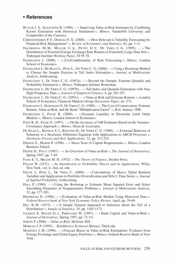
To derive the out of sample (P,Q) estimator consider two excess probabili-ties p and t with p < 1/n < t, where n is the sample size. Corresponding to pand t are the large quantiles, xp and xt, where for xi we have 1 − F(xi ) = i,i = t,p. Using the expansion of F(x) in (8) with β > 0, ignoring the higherorder terms in the expansion, and replacing t by M/n and xt by the (M + 1)-th descending order statistic one obtains the estimator

(10) x̂p = X(M+1)

(m

np

) 1α̂

.

It can be shown that the quantile estimator x̂p is asymptotically normallydistributed. A reverse estimator can be developed as well by a similar manipu-lation of (8)

(11) p̂ = M

n

(xt

xp

)α̂

.

The excess probability estimator p̂ is also asymptotically normally distri-buted.

262

APPENDIX B

Figures and Tables


TABLE 1Daily SP-500, 1990-96. Time Between Extreme Returns

Upper Tail Lower Tail

date days rank date days rank

90-08-27 74 2 90-01-23 6 690-10-01 24 4 90-08-07 136 390-10-18 13 8 90-08-17 8 1290-10-19 1 10 90-08-22 3 1590-11-09 15 14 90-08-24 2 491-01-17 46 1 90-09-25 21 1491-02-06 14 16 90-10-10 11 591-02-11 3 5 91-05-13 148 1791-03-05 15 13 91-08-20 69 1091-04-02 19 9 91-11-18 63 191-08-21 99 3 93-02-17 315 991-12-23 86 6 93-04-05 33 1691-12-30 4 11 94-02-07 214 1193-03-08 300 17 96-03-11 527 294-04-05 273 12 96-07-08 82 1396-12-19 686 15 96-07-16 6 7

TABLE 2Predicted and Expected Maxima of Student-t (4)

In Sample Prediction, Theoretical Average Values2000 observations

Sample Maxima by HS 8.610 10.67 (4.45) [4.90]Forecast Maximas by EV 8.610 8.90 (1.64) [1.66]

Out of Sample Prediction

Forecast Maximas by EV 10.306 10.92 (2.43) [2.50]for Sample of Size 4000Forecast Maximas by EV 11.438 12.32 (3.02) [3.14]for Sample of Size 6000

Sample size = 2,000, simulations 1,000, bootstrap iterations = 2,000. Standard errors in parenthesis,RMSE in brackets. HS denotes estimation by historical simulation and EV estimation with the methodproposed by DANIELSSON and DE VRIES [1997b].

264

TABLE 3Extreme Daily returns 1987-1996

JPM 25 % 12 % 8.8 % 6.7 % 6.5 % 6.4 % 6.3 %– 41 % – 6.7 % – 6.3 % – 6.1 % – 6.0 % – 5.8 % – 5.7 %

MMM 11 % 7.1 % 5.9 % 5.7 % 5.7 % 5.0 % 4.8 %– 30 % – 10 % – 10 % – 9.0 % – 6.2 % – 6.1 % – 5.6 %

MCD 10 % 7.9 % 6.3 % 6.2 % 5.4 % 5.0 % 5.0 %– 18 % – 10 % – 8.7 % – 8.5 % – 8.3 % – 7.3 % – 6.9 %

INTC 24 % 11 % 9.9 % 9.0 % 8.9 % 8.6 % 8.6 %– 21 % – 21 % – 16 % – 15 % – 14 % – 12 % – 12 %

IBM 12 % 11 % 11 % 10 % 9.4 % 7.4 % 6.5 %– 26 % – 11 % – 11 % – 9.3 % – 7.9 % – 7.5 % – 7.1 %

XRX 12 % 8.0 % 7.8 % 7.5 % 7.1 % 6.8 % 6.3 %– 22 % – 16 % – 11 % – 8.4 % – 7.5 % – 6.9 % – 6.2 %

XON 17 % 10 % 6.0 % 5.8 % 5.8 % 5.6 % 5.4 %– 27 % – 8.7 % – 7.9 % – 6.6 % – 6.3 % – 5.7 % – 5.4 %

SP-500 8.7 % 5.1 % 4.8 % 3.7 % 3.5 % 3.4 % 3.3 %– 23 % – 8.6 % – 7.0 % – 6.3 % – 5.3 % – 4.5 % – 4.3 %

TABLE 4Observed Extreme Returns of the daily SP-500, 1990-1996, and theProbability of that Return as Predicted by the Normal GARCH, Student-tGARCH Model, the Extreme Value Estimation Method, and the EmpiricalDistribution. Due to Moving Estimation Windows Results RepresentDifferent Samples

Observed Probabilities

Return Normal Student-t EV Estimator Empirical

– 3.72 % 0.0000 0.0002 0.0007 0.0006– 3.13 % 0.0000 0.0010 0.0015 0.0011– 3.07 % 0.0002 0.0021 0.0016 0.0017– 3.04 % 0.0032 0.0071 0.0016 0.0023– 2.71 % 0.0098 0.0146 0.0026 0.0028– 2.62 % 0.0015 0.0073 0.0029 0.0034

3.66 % 0.0000 0.0011 0.0004 0.00063.13 % 0.0060 0.0096 0.0009 0.00112.89 % 0.0002 0.0022 0.0013 0.00172.86 % 0.0069 0.0117 0.0014 0.00232.53 % 0.0059 0.0109 0.0025 0.00282.50 % 0.0007 0.0038 0.0026 0.0034


TABLE 510 Day VaR Prediction on December 30, 1996 in Millions of US Dollars fora $100 Million Trading Portfolio

Risk Level 5 % 1.0 % 0.5 % 0.10 % 0.05 % 0.005 %

EVOne day $0.9 $1.5 $1.7 $2.5 $3.0 $5.110 day $1.6 $2.5 $3.0 $4.3 $5.1 $8.9

RMOne day $1.0 $1.4 $1.6 $1.9 $2.0 $2.310 day $3.2 $4.5 $4.9 $5.9 $6.3 $7.5

TABLE 6Effect of Inclusion of Option in Portfolio

Confidence Level VaR with Option VaR without Option Difference

95 % $895,501 $1,381,519 $486,01999 % $1,474,056 $2,453,564 $979,50899.5 % $1,823,735 $2,754,562 $930,82799.9 % $3,195,847 $3,856,747 $669,90099.99 % $7,130,721 $6,277,714 – $853,007

TABLE 7Summary Statistics. Jan. 27, 1984 to Dec. 31, 1996

JPM MMM MCD INTC IBM XRX XON

Mean 0.05 0.04 0.07 0.09 0.01 0.04 0.05S.D. 1.75 1.41 1.55 2.67 1.62 1.62 1.39Kurtosis 100.28 68.07 8.36 5.88 25.71 16.44 49.23Skewness – 2.70 – 3.17 – 0.58 – 0.36 – 1.08 – 1.06 – 1.74Minimum – 40.56 – 30.10 – 18.25 – 21.40 – 26.09 – 22.03 – 26.69Maximum 24.63 10.92 10.05 23.48 12.18 11.67 16.48

Note: JPM = J. P. Morgan; MMM = 3m; MCD = McDonalds; INTC = Intel; IBM = IBM;XRX = Xerox; XON = Exxon.Source: DATASTREAM

TABLE 8Summary Statistics. Jan. 2, 1990 to Dec. 31, 1996


Mean 0.05 0.04 0.05 0.15 0.03 0.06 0.04S.D. 1.45 1.19 1.48 2.34 1.72 1.60 1.12Kurtosis 1.83 3.78 1.51 2.86 6.67 9.46 1.10Skewness 0.28 – 0.32 0.05 – 0.36 0.25 – 0.35 0.11Minimum – 6.03 – 9.03 – 8.70 – 14.60 – 11.36 – 15.63 – 4.32Maximum 6.70 4.98 6.27 9.01 12.18 11.67 5.62

TABLE 9Correlation Matrix. Jan. 27, 1984 to Dec. 31, 1996


JPM 1.00MMM 0.49 1.00MCD 0.42 0.44 1.00INTC 0.30 0.36 0.29 1.00IBM 0.38 0.42 0.34 0.40 1.00XRX 0.35 0.39 0.34 0.32 0.35 1.00XON 0.44 0.48 0.37 0.24 0.35 0.30 1.00

TABLE 10Correlation Matrix. Jan. 2, 1990 to Dec. 31, 1996


JPM 1.00MMM 0.28 1.00MCD 0.28 0.28 1.00INTC 0.24 0.21 0.21 1.00IBM 0.18 0.19 0.19 0.32 1.00XRX 0.23 0.23 0.22 0.21 0.19 1.00XON 0.20 0.25 0.21 0.12 0.10 0.12 1.00

266


Tail

Perc

enta

ge0.

005

%0.

01%

0.02

5%

0.05

%0.

1%

0.25

%0.

5%

1%

2.5

%5

%E

xpec

ted

0.05

0.1

0.25

0.5

12.

55

1025

50

Freq

uenc

y D

ays

200

100

4020

Freq

uenc

y Y

ears

7738

157.

73.

81.

5

Ris

kMet

rics

1.58

2.00

2.72

3.55

4.85

7.29

10.6

516

.28

30.2

652

.45

(1.2

9)(1

.45)

(1.6

6)(1

.81)

(2.0

6)(2

.27)

(2.7

3)(3

.13)

(4.4

1)(7

.39)

His

tori

cal

0.75

0.75

0.75

0.75

0.95

1.90

3.69

7.66

20.5

043

.24

Sim

ulat

ion

(0.8

9)(0

.89)

(0.8

9)(0

.89)

(1.0

3)(1

.57)

(2.3

9)(3

.90)

(7.2

2)(1

0.75

)

Tail

Ker

nel

0.09

0.09

0.37

0.68

1.21

2.54

4.82

9.32

22.3

544

.02

Pres

ampl

ing

(0.3

1)(0

.31)

(0.7

1)(0

.98)

(1.2

7)(1

.71)

(2.5

6)(4

.26)

(7.6

6)(1

1.62

)

Tail

Ker

nel

0.06

0.12

0.33

0.59

1.06

2.35

4.23

8.19

20.8

443

.14

Post

-Fitt

ing

(0.2

3)(0

.35)

(0.6

2)(0

.82)

(1.1

3)(1

.72)

(2.5

5)(3

.86)

(7.3

5)(

11.1

0)

TAB

LE

11E

stim

atio

n R

esul

ts. A

vera

ge n

umbe

r of

rea

lized

por

tfol

ios

that

wer

e la

rger

than

VaR

Pre

dict

ions

Obs

erva

tion

s in

tes

ting

= 1

,000

ove

r pe

riod

930

115

to 9

6123

0. W

indo

w s

ize

in H

S an

d E

K-H

S =

1,5

00, i

niti

al s

tart

ing

date

for

win

dow

870

210,

ran

dom

por

tfol

ios

= 5

00, s

imul

a-ti

on s

ize

in H

S-ex

trem

e ke

rnel

= 1

0,00

0. S

tand

ard

erro

rs i

n pa

rent

hesi

s.

uppe

r ta

illo

wer

tail

mea

nva

rku

rtos

ism

axm

insk

ewα

mX

(m+1

)m

axα

mX

(m+1

)m

ax

Stoc

k In

dex

Han

g Se

ng0.

062.

714

4.5

8.9

–40

.5–

6.5

3.5

323.

53.

6%

2.2

49–

3.2

–3.

3%

Stra

ight

s T

imes

0.03

1.5

64.4

11.5

–23

.4–

3.7

3.1

362.

52.

6%

2.2

59–

2.3

–2.

3%

Wor

d0.

030.

625

.77.

9–

10.0

–1.

43.

537

1.6

1.7

%3.

144

–1.

6–

1.7

%D

AX

0.03

1.4

12.2

7.3

–13

.7–

1.1

2.9

522.

32.

3%

2.6

43–

2.7

–2.

8%

FTA

ll Sh

are

0.03

0.7

25.9

5.7

–12

.1–

2.0

2.9

581.

51.

5%

3.1

86–

1.3

–1.

3%

SP-5

000.

041.

011

5.8

8.7

–22

.8–

5.1

3.8

262.

32.

4%

2.5

51–

1.9

–1.

9%

Mis

cella

neou

s A

sset

s

Gol

d B

ulio

n0.

000.

57.

63.

6–

7.2

–1.

04.

816

2.2

2.2

%3.

033

–1.

9–

1.9

%U

S B

onds

0.00

0.9

73.5

17.8

–10

.71.

72.

486

1.3

1.4

%2.

579

–1.

4–

1.5

%

US

Stoc

ks

JPM

0.03

3.3

106.

924

.6–

40.6

–3.

13.

531

4.2

4.3

%3.

148

–3.

2–

3.3

%M

MM

0.04

2.1

72.5

10.9

–30

.1–

3.6

4.5

293.

43.

5%

2.4

52–

2.8

–2.

9%

MC

D0.

062.

56.

610

.0–

18.3

–0.

75.

222

4.1

4.2

%3.

045

–3.

3–

3.4

%IN

TC

0.13

6.8

5.1

23.5

–21

.4–

0.5

4.7

296.

36.

6%

2.8

37–

6.2

–6.

4%

IBM

0.01

2.9

23.5

12.2

–26

.1–

1.2

3.2

284.

34.

5%

2.9

38–

3.8

–3.

9%

XR

X0.

032.

616

.911

.7–

22.0

–1.

23.

629

4.0

4.1

%2.

750

–3.

3–3

.4%

XO

N0.

042.

056

.716

.5–

26.7

–2.

03.

534

3.1

3.2

%2.

770

–2.

3–

2.4

%

Fore

x

FRF/

USD

–0.

010.

4–

0.8

2.7

–3.

20.

06.

216

2.0

2.0

%8.

217

–2.

1–

2.1

%D

M/U

SD–

0.01

0.5

–0.

93.

2–

3.0

0.0

7.0

162.

22.

2%

6.7

16–

2.1

–2.

2%

YE

N/U

SD–

0.01

0.4

0.2

3.4

–3.

6–

0.2

4.9

161.

92.

0%

4.7

18–

2.1

–2.

1%

GB

P/U

SD–

0.01

0.4

–0.

53.

3–

2.8

0.3

9.5

162.

32.

3%

6.3

17–

1.9

–2.

0%

TAB

LE

1210

Yea

rs, 2

,600

Dai

ly R

etur

ns, 1

987-

1996

. With

Pre

dict

ed M

axim

um D

aily

Dro

p in

one

Yea

r (2

50 d

ays)

268


FIGURE 11 % Largest and Smallest Daily Returns on Stocks in Portfolio

(a) J. P. Morgan (b) 3M

(c) McDonalds (d) Intel

(e) IBM (f) Xerox

(h) SP-500(g) Exxon

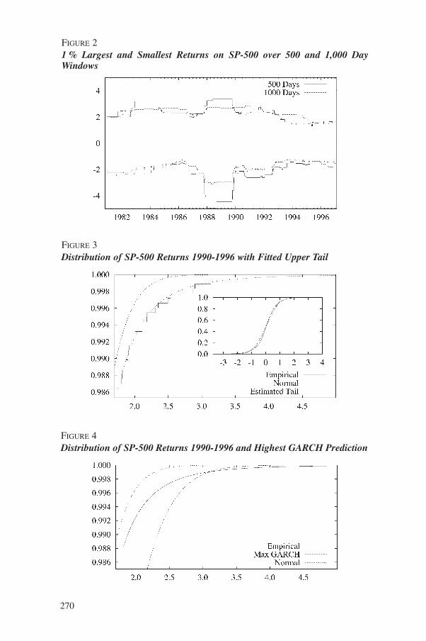
FIGURE 21 % Largest and Smallest Returns on SP-500 over 500 and 1,000 DayWindows

FIGURE 3Distribution of SP-500 Returns 1990-1996 with Fitted Upper Tail

FIGURE 4Distribution of SP-500 Returns 1990-1996 and Highest GARCH Prediction

270

value-at-risk and extreme returns - repub

Documents