validation of the recipe for broadband ground-motion ... of the recipe for broadband ground-motion...
TRANSCRIPT

Validation of the Recipe for Broadband Ground-Motion
Simulations of Japanese Crustal Earthquakes
by Asako Iwaki, Takahiro Maeda, Nobuyuki Morikawa, Hiroe Miyake,* and Hiroyuki Fujiwara
Abstract The robustness of broadband ground-motion simulation can promoteseismic-hazard assessment. A broadband ground-motion simulation technique called“the recipe” is used in the scenario earthquake shaking maps of the National SeismicHazard Maps for Japan. The recipe represents a fault rupture based on a multipleasperity model referred to as the characterized source model. Broadband ground-motion time histories on the engineering bedrock are computed by a hybrid approachof the 3D finite-difference method and the stochastic Green’s function method for thelong- (>1 s) and short-period (<1 s) ranges, respectively, using a 3D velocity struc-ture model. The ground motion on the ground surface is computed using the 1D siteresponse of the surface soil layers. Because the need for ground-motion simulations ofscenario earthquakes is increasing, it is important to validate the method from seis-mological and engineering perspectives. This study presents a validation of the recipeusing velocity waveforms, peak ground velocity (PGV), seismic intensity, and pseu-doacceleration response spectra. The validation scheme follows the framework of theSouthern California Earthquake Center Broadband Platform. We selected twoMw 6.6crustal earthquakes that occurred in Japan as the targets of this study: the 2000 Tottoriand the 2004 Chuetsu (mid-Niigata) earthquakes. The validation results are satisfac-tory except for those in the shortest-period range (0.01–0.1 s) at large hypocentraldistances (>70 km); such conditions are outside of the target range of the recipe.Simulations using a 1D velocity structure model were also examined. The simulationresults for the 1D and 3D velocity structure models indicated that the 3D velocitystructure models are important in reproducing PGV and the later phases with longduration, especially on deep sediment sites.
Introduction
Prediction of broadband ground motion for scenarioearthquakes requires numerous processes including model-ing the fault rupture, wave propagation, and site responsewithin the near-surface soil structure. Such ground-motionprediction will be important for precise seismic-hazard as-sessments in modern society. Reproducibility of broadbandground motion by third-party researchers has become an im-portant requirement. The Southern California EarthquakeCenter (SCEC) worked to solve this issue and establishedthe Broadband Platform (BBP) (e.g., Maechling et al., 2015).This is an ideal open-source tool that allows the integrationof several rupture-generator models and ground-motion sim-ulation techniques (e.g., Motazedian and Atkinson, 2005;Graves and Pitarka, 2010; Olsen and Takedatsu, 2015). Inthe current SCEC BBP version, most fault rupture models
are based on random slip realization or the k-squared slipdistribution in the wavenumber domain. Their main objectiveis to perform a huge amount of ground-motion simulationswith random source parameters. The Green’s functions arebased on 1D velocity structure models specified by the user.The ground-motion simulation methods are validated bycomparing the simulated ground motion with the observedground motion for past earthquakes or ground-motion pre-diction equations (GMPEs) for scenario earthquakes, usingcriteria for pseudoacceleration response spectra (PSA) (Gou-let et al., 2015). Lately, many works focus on validation ofground-motion prediction methods; a number of papers referto the criteria used in the SCEC BBP validation (e.g., Booreet al., 2014; Sun et al., 2015).
The Earthquake Research Committee (ERC) of theHeadquarters for Earthquake Research Promotion (HERP) ofJapan has developed a broadband ground-motion simula-tion method that integrates the characterized source modeland the 3D velocity structure model into a standard
*Also at Earthquake Research Institute, The University of Tokyo, 1-1-1Yayoi, Bunkyo-ku, Tokyo 113-0032, Japan.
2214
Bulletin of the Seismological Society of America, Vol. 106, No. 5, pp. 2214–2232, October 2016, doi: 10.1785/0120150304
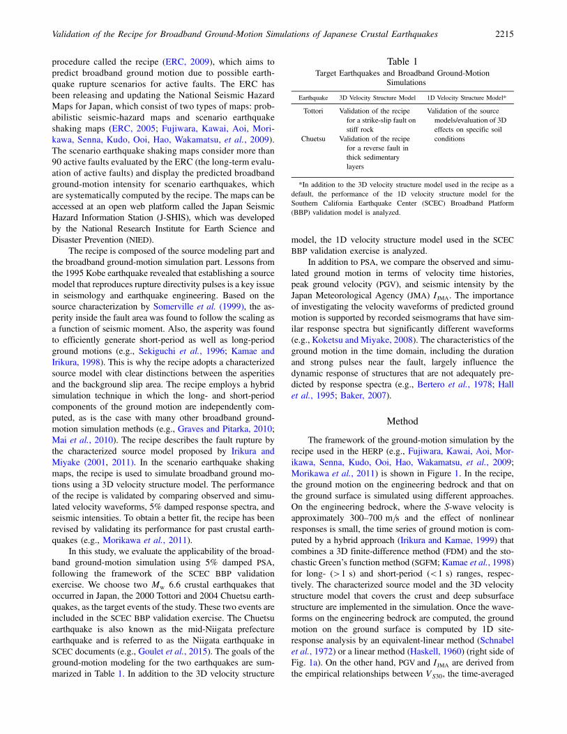
procedure called the recipe (ERC, 2009), which aims topredict broadband ground motion due to possible earth-quake rupture scenarios for active faults. The ERC hasbeen releasing and updating the National Seismic HazardMaps for Japan, which consist of two types of maps: prob-abilistic seismic-hazard maps and scenario earthquakeshaking maps (ERC, 2005; Fujiwara, Kawai, Aoi, Mori-kawa, Senna, Kudo, Ooi, Hao, Wakamatsu, et al., 2009).The scenario earthquake shaking maps consider more than90 active faults evaluated by the ERC (the long-term evalu-ation of active faults) and display the predicted broadbandground-motion intensity for scenario earthquakes, whichare systematically computed by the recipe. The maps can beaccessed at an open web platform called the Japan SeismicHazard Information Station (J-SHIS), which was developedby the National Research Institute for Earth Science andDisaster Prevention (NIED).
The recipe is composed of the source modeling part andthe broadband ground-motion simulation part. Lessons fromthe 1995 Kobe earthquake revealed that establishing a sourcemodel that reproduces rupture directivity pulses is a key issuein seismology and earthquake engineering. Based on thesource characterization by Somerville et al. (1999), the as-perity inside the fault area was found to follow the scaling asa function of seismic moment. Also, the asperity was foundto efficiently generate short-period as well as long-periodground motions (e.g., Sekiguchi et al., 1996; Kamae andIrikura, 1998). This is why the recipe adopts a characterizedsource model with clear distinctions between the asperitiesand the background slip area. The recipe employs a hybridsimulation technique in which the long- and short-periodcomponents of the ground motion are independently com-puted, as is the case with many other broadband ground-motion simulation methods (e.g., Graves and Pitarka, 2010;Mai et al., 2010). The recipe describes the fault rupture bythe characterized source model proposed by Irikura andMiyake (2001, 2011). In the scenario earthquake shakingmaps, the recipe is used to simulate broadband ground mo-tions using a 3D velocity structure model. The performanceof the recipe is validated by comparing observed and simu-lated velocity waveforms, 5% damped response spectra, andseismic intensities. To obtain a better fit, the recipe has beenrevised by validating its performance for past crustal earth-quakes (e.g., Morikawa et al., 2011).
In this study, we evaluate the applicability of the broad-band ground-motion simulation using 5% damped PSA,following the framework of the SCEC BBP validationexercise. We choose two Mw 6.6 crustal earthquakes thatoccurred in Japan, the 2000 Tottori and 2004 Chuetsu earth-quakes, as the target events of the study. These two events areincluded in the SCEC BBP validation exercise. The Chuetsuearthquake is also known as the mid-Niigata prefectureearthquake and is referred to as the Niigata earthquake inSCEC documents (e.g., Goulet et al., 2015). The goals of theground-motion modeling for the two earthquakes are sum-marized in Table 1. In addition to the 3D velocity structure
model, the 1D velocity structure model used in the SCECBBP validation exercise is analyzed.
In addition to PSA, we compare the observed and simu-lated ground motion in terms of velocity time histories,peak ground velocity (PGV), and seismic intensity by theJapan Meteorological Agency (JMA) IJMA. The importanceof investigating the velocity waveforms of predicted groundmotion is supported by recorded seismograms that have sim-ilar response spectra but significantly different waveforms(e.g., Koketsu and Miyake, 2008). The characteristics of theground motion in the time domain, including the durationand strong pulses near the fault, largely influence thedynamic response of structures that are not adequately pre-dicted by response spectra (e.g., Bertero et al., 1978; Hallet al., 1995; Baker, 2007).
Method
The framework of the ground-motion simulation by therecipe used in the HERP (e.g., Fujiwara, Kawai, Aoi, Mor-ikawa, Senna, Kudo, Ooi, Hao, Wakamatsu, et al., 2009;Morikawa et al., 2011) is shown in Figure 1. In the recipe,the ground motion on the engineering bedrock and that onthe ground surface is simulated using different approaches.On the engineering bedrock, where the S-wave velocity isapproximately 300–700 m=s and the effect of nonlinearresponses is small, the time series of ground motion is com-puted by a hybrid approach (Irikura and Kamae, 1999) thatcombines a 3D finite-difference method (FDM) and the sto-chastic Green’s function method (SGFM; Kamae et al., 1998)for long- (>1 s) and short-period (<1 s) ranges, respec-tively. The characterized source model and the 3D velocitystructure model that covers the crust and deep subsurfacestructure are implemented in the simulation. Once the wave-forms on the engineering bedrock are computed, the groundmotion on the ground surface is computed by 1D site-response analysis by an equivalent-linear method (Schnabelet al., 1972) or a linear method (Haskell, 1960) (right side ofFig. 1a). On the other hand, PGV and IJMA are derived fromthe empirical relationships between VS30, the time-averaged
Table 1Target Earthquakes and Broadband Ground-Motion
Simulations
Earthquake 3D Velocity Structure Model 1D Velocity Structure Model*
Tottori Validation of the recipefor a strike-slip fault onstiff rock
Validation of the sourcemodels/evaluation of 3Deffects on specific soilconditionsChuetsu Validation of the recipe
for a reverse fault inthick sedimentarylayers
*In addition to the 3D velocity structure model used in the recipe as adefault, the performance of the 1D velocity structure model for theSouthern California Earthquake Center (SCEC) Broadband Platform(BBP) validation model is analyzed.
Validation of the Recipe for Broadband Ground-Motion Simulations of Japanese Crustal Earthquakes 2215

S-wave velocity to a depth of 30 m, and the amplificationfactors of PGVand IJMA (left side of Fig. 1a; see the Appendixfor detail).
Characterized Source Models
The recipe employs the characterized source model(Irikura and Miyake, 2001, 2011) to model the fault ruptureof crustal earthquakes. The characterized source model is
composed of multiple asperities and the surrounding back-ground area, where the asperities are defined as regions, orpatches, that have a larger slip than the average slip of theentire rupture area. Following Das and Kostrov (1986), asper-ities with large slips generate long-period as well as short-period seismic-wave radiations due to large stress drop. Thebackground area with a stress-free field also generateslong-period seismic-wave radiation. The scaling relationshipsof the rupture areas of the entire fault and asperities with
Figure 1. (a) Flow diagram for the broadband ground-motion simulations following the recipe (modified fromMorikawa et al., 2011; a boxfor pseudoacceleration response spectra [PSA] RotD50 was added in this study). (b) Schematic illustration showing the velocity structure (fromFujiwara, Kawai, Aoi, Morikawa, Senna, Kudo, Ooi, Hao, Wakamatsu, et al., 2009). The 3D velocity structure model covers the crust and deepvelocity structure, and the surface soil layers correspond to the velocity structure between the engineering bedrock and the ground surface.
2216 A. Iwaki, T. Maeda, N. Morikawa, H. Miyake, and H. Fujiwara

respect to the total seismic moment are used to derive threekinds of parameters: the outer, inner, and extra fault parame-ters. The outer fault parameters define the size, configuration,and seismic moment of the entire rupture area. The inner faultparameters describe the heterogeneity of the slip within thefault: the size, seismic moment, and the stress drop of theasperities. The extra fault parameters include the rupture start-ing point and the rupture velocity. The procedures for derivingthe fault parameters used in the HERP are described inFujiwara, Kawai, Aoi, Morikawa, Senna, Kudo, Ooi, Hao,Wakamatsu, et al. (2009) and Morikawa et al. (2011). Thecharacterized source model well reproduces the rupture direc-tivity pulse (e.g., Somerville et al., 1997), which enhances theresponse spectra, as in the 1995 Kobe earthquake.
In the recipe, information from the long-term evaluationof active faults by the HERP is used to set the location of therupture fault as well as those of the asperities whenever pos-sible. If such information is not available, the recipe recom-
mends considering several patterns of asperity locationsand rupture nucleation points. In this study, we assume thatthe approximate fault configuration, asperity locations, andthe rupture starting point are roughly known, allowing thesource characterization and ground-motion simulation proc-esses to be validated. Although the recipe provides the basicprocedure to derive the parameters following the scalingrelationships, it also recommends incorporating other geo-logical, seismological, or engineering information that isconsidered better suited to a specific situation. Therefore,we present two and four cases for the Tottori and Chuetsuearthquakes, respectively, using different fault parameters.The fault configurations are shown in Figure 2, and the faultparameters are given in Tables 2 and 3, which are describedin more detail in later paragraphs. The Kostrov-like slip timefunction is given by the formulation of Nakamura and Miya-take (2000). The rupture front propagates from the hypocen-ter with a constant rupture velocity VR. The fault is spatially
Case1 Case2
asp.2
asp.1
26 km
2 km
14 km
S150°E
dip 90º
asp.2
asp.1
S150°E
dip 90°
(a)
Case1
Case3
Case2
Case4
26 km
16 km
N215°E
asp.1
(b)
dip 50°
4 km
N215°E
dip 50°
N215°E
dip 50°
N215°E
dip 50°
asp.2
asp.1
asp.3
asp.1asp.2
asp.1 asp.2
Figure 2. Configuration of the characterized source models for the (a) Tottori and (b) Chuetsu earthquakes with 2 km grid lines. Thehorizontal and vertical directions correspond to the directions along strike and dip, respectively. More detailed parameters are listed inTables 2 and 3.
Validation of the Recipe for Broadband Ground-Motion Simulations of Japanese Crustal Earthquakes 2217

discretized into 0:5 × 0:5 and 2:0 × 2:0 km2 subfaults forFDM and SGFM, respectively.
3D Velocity Structure Models
The recipe employs three types of velocity structuremodels: the crustal structure of the seismic bedrock anddeeper, the deep subsurface structure, and the shallow sub-surface structure as shown in Figure 1b. The crustal structuremodel and the deep subsurface structure model are used tocompute the waveforms on the engineering bedrock, whereasthe shallow subsurface structure model is used to computethose on the ground surface. The velocity structure modelis described in detail by Fujiwara, Kawai, Aoi, Morikawa,Senna, Kudo, Ooi, Hao, Hayakawa, et al. (2009), and also
briefly by Fujiwara, Kawai, Aoi, Morikawa, Senna, Kudo,Ooi, Hao, Wakamatsu, et al. (2009).
The 3D crustal structure model that extends from theupper crust to the mantle is attached to the deep subsurfacestructure and is based on the tomography model of Matsubaraet al. (2008). The 3D deep subsurface structure is based on v.2of the J-SHIS velocity structure model (J-SHIS V2) (Fujiwara,Kawai, Aoi, Morikawa, Senna, Kudo, Ooi, Hao, Hayakawa,et al., 2009; see Data and Resources for reference). It spans thestructure between the seismic bedrock (VS ∼ 3000 m=s) andthe engineering bedrock (VS ∼ 500–1000 m=s). The physicalproperties of the bedrock vary depending on the geologicalconditions. The first three layers (VS < 500 m=s) are excludedin this study to reduce the computational cost because they aremodeled only in limited small areas of Japan.
The shallow subsurface structure is constructed based onthe 250-m-grid Japan engineering geomorphologic classifi-cation map of Wakamatsu and Matsuoka (2013). The distri-bution of VS30 is estimated from the map, considering thegeomorphologic classification, elevation, slope gradient, anddistance from mountains and hills.
Broadband Ground Motion on the EngineeringBedrock by a Hybrid Approach
As mentioned previously, the time series of the broad-band ground motion on the engineering bedrock is computedby a hybrid approach of 3D FDM and SGFM for long- (>1 s)and short-period (<1 s) ranges, respectively. The procedureof the hybrid approach is described in detail by Fujiwara,Kawai, Aoi, Morikawa, Senna, Kudo, Ooi, Hao, Wakamatsu,et al. (2009) and Morikawa et al. (2011).
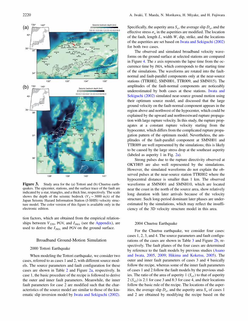
The long-period component is computed by the 3D FDMusing discontinuous grids (Aoi and Fujiwara, 1999), whichruns on an open-source code called Ground Motion Simulator(Aoi et al., 2004). The rupture and wave propagation effectsare incorporated into the FDM computation using the charac-terized source model and the J-SHIS V2 3D velocity structuremodel. Figure 3a,b shows the depth distribution of the seismicbedrock (VS ∼ 3000 m=s) in the study area for the Tottori andChuetsu earthquakes, respectively. The source area of theTottori earthquake is on a stiff rock site, whereas that of theChuetsu earthquake is on significantly deep sedimentarylayers. The depth of the sedimentary layers varies spatially andextends to a maximum of nearly 10 km. The minimum VS isset to 500 m=s, and the grid spacing is set to 80 m at depthssmaller than 2 and 8 km for the Tottori and Chuetsu earth-quakes, respectively, to ensure accuracy up to the crossoverperiod of 1 s. The grid spacing is set to 240 m in the deeperregion. In the FDM computation,Q-value is given byQ�f � �QSf=f0 in which f0 � 1 Hz and QS is the reference Q-valuefor S wave.
The short-period component is computed by the SGFMcode of Dan and Sato (1998). In the SGFM, the stochasticground motion following the ω−2 source model (Boore,1983) of a small earthquake, or the SGF, is synthesized on
Table 2Source Parameters for the Tottori Earthquake
Unit Case 1 Case 2
Length L* km 27(26)Width W* km 15(14)Latitude, longitude at topcenter
degrees (°) 35.27, 133.34
Strike degrees (°) N150EDip degrees (°) 90Rake degrees (°) 180Depth to top km 2.0Total seismic moment M0 N·m 9:12 × 1018
Mw 6.6Short-period level A† N·m=s=s 1:11 × 1019
Average slip D m 0.68Rupture velocity m=s 2500Hypocenter depth alongdip
km 12‡ 8§
Asperity area Sa km2 52 108§
Asperity 1Area Sa1* km2 35�6 × 6� 54�6 × 8�§Seismic moment M0a1 N·m 1:8 × 10¹⁸ 3:9 × 10¹⁸
Effective stress σa1 MPa 21.1 16.0§
Average slip Da1 m 1.51 2.21§
Rise time tr s 1.18 1.47Asperity 2Area Sa2* km2 18�6 × 4� 54�8 × 6�§Seismic moment M0a2 N·m 6:2 × 10¹⁷ 3:9 × 10¹⁸
Effective stress σa2 MPa 21.1 11.3§
Average slip Da2 m 1.07 2.21§
Rise time tr s 0.84 1.47Background areaArea Sb km2 338 297Seismic moment M0b N·m 6:8 × 10¹⁸ 1:7 × 10¹⁸
Effective stress σb MPa 3.2 1.6Average slip Db m 0.6 0.13Rise time tr s 3.8 3.4
Locations of the asperities are shown in Figure 2a.*Lengths and widths of the fault and the asperities that are adjusted to the
2 km × 2 km subfaults are denoted in the parentheses.†Acceleration source spectral amplitude at short periods inferred from the
empirical relation with seismic moment by Dan et al. (2001).‡Hypocenter depth from the top of the fault along dip by Goulet
et al. (2015).§Estimated from Iwata and Sekiguchi (2002).
2218 A. Iwaki, T. Maeda, N. Morikawa, H. Miyake, and H. Fujiwara
the engineering bedrock. Then, the SGF is summed over thefault of a large earthquake based on the self-similar scalingrelations and the ω−2 source spectral model in a similar man-ner as in the empirical Green’s function method (Irikura,1986). The horizontal and vertical components are computedby considering SH and SV waves, respectively, with verticalincident, using a 1D velocity structure extracted from theJ-SHIS V2 3D velocity structure model at each site. Theempirical vertical-to-horizontal spectral ratio proposed byNishimura et al. (2001) is used to adjust the amplitude of thevertical component.
The long- and short-period components are superposi-tioned in the time domain to create a time series of a broadbandground motion at the crossover period (1 s) after applying apair of high- and low-cut filters. The sampling frequency is
200 Hz for both the long- and short-period components. Weapplied high-cut filter at 30 Hz to the broadband waveforms.
Broadband Ground Motion on the Ground Surface
As shown in Figure 1a, the recipe recommends twomethods to simulate the ground motion on the ground sur-face. In this study, we take the method on the right side ofFigure 1 to compute the velocity time series by the 1D site-response analysis (Haskell, 1960) using the surface soillayers estimated from the logging data of K-NET and KiK-net. On the other hand, we compute PGV and IJMA based onthe empirical relationship between VS30, PGV, and IJMA (leftside of Fig. 1a). First, IJMA and PGV are calculated from thewaveforms on the engineering bedrock. Then, the amplifica-
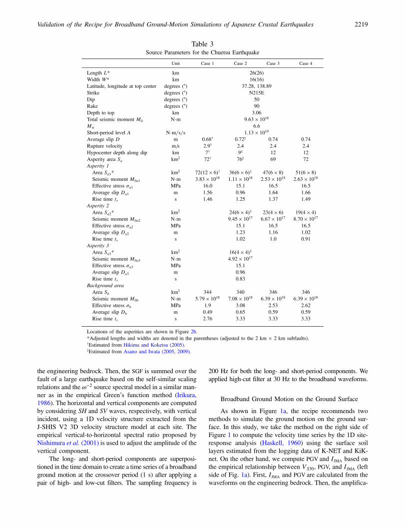
Table 3Source Parameters for the Chuetsu Earthquake
Unit Case 1 Case 2 Case 3 Case 4
Length L* km 26(26)Width W* km 16(16)Latitude, longitude at top center degrees (°) 37.28, 138.89Strike degrees (°) N215EDip degrees (°) 50Rake degrees (°) 90Depth to top km 3.06Total seismic moment M0 N·m 9:63 × 1018
Mw 6.6Short-period level A N·m=s=s 1:13 × 1019
Average slip D m 0.68† 0.72‡ 0.74 0.74Rupture velocity m=s 2.9† 2.4 2.4 2.4Hypocenter depth along dip km 7† 9‡ 12 12Asperity area Sa km2 72† 76‡ 69 72Asperity 1Area Sa1* km2 72�12 × 6�† 36�6 × 6�‡ 47�6 × 8� 51�6 × 8�Seismic moment M0a1 N·m 3:83 × 1018 1:11 × 1018 2:53 × 1018 2:63 × 1018
Effective stress σa1 MPa 16.0 15.1 16.5 16.5Average slip Da1 m 1.56 0.96 1.64 1.66Rise time tr s 1.46 1.25 1.37 1.49
Asperity 2Area Sa2* km2 24�6 × 4�‡ 23�4 × 6� 19�4 × 4�Seismic moment M0a2 N·m 9:45 × 1017 6:67 × 1017 8:70 × 1017
Effective stress σa2 MPa 15.1 16.5 16.5Average slip Da2 m 1.23 1.16 1.02Rise time tr s 1.02 1.0 0.91
Asperity 3Area Sa3* km2 16�4 × 4�‡Seismic moment M0a3 N·m 4:92 × 1017
Effective stress σa3 MPa 15.1Average slip Da3 m 0.96Rise time tr s 0.83
Background areaArea Sb km2 344 340 346 346Seismic moment M0b N·m 5:79 × 1018 7:08 × 1018 6:39 × 1018 6:39 × 1018
Effective stress σb MPa 1.9 3.08 2.53 2.62Average slip Db m 0.49 0.65 0.59 0.59Rise time tr s 2.76 3.33 3.33 3.33
Locations of the asperities are shown in Figure 2b.*Adjusted lengths and widths are denoted in the parentheses (adjusted to the 2 km × 2 km subfaults).†Estimated from Hikima and Koketsu (2005).‡Estimated from Asano and Iwata (2005, 2009).
Validation of the Recipe for Broadband Ground-Motion Simulations of Japanese Crustal Earthquakes 2219
tion factors, which are obtained from the empirical relation-ships between VS30, PGV, and IJMA (see the Appendix), areused to derive the IJMA and PGV on the ground surface.
Broadband Ground-Motion Simulation
2000 Tottori Earthquake
When modeling the Tottori earthquake, we consider twocases, referred to as cases 1 and 2, with different source mod-els. The source parameters and fault configuration for thesecases are shown in Table 2 and Figure 2a, respectively. Incase 1, the basic procedure of the recipe is followed to derivethe outer and inner fault parameters. Meanwhile, the innerfault parameters for case 2 are modified such that the char-acteristics of the source model are similar to those of the kin-ematic slip inversion model by Iwata and Sekiguchi (2002).
Specifically, the asperity area Sa, the average slipDa, and theeffective stress σa in the asperities are modified. The locationof the fault, length L, width W, dip, strike, and the locationsof the asperities are set based on Iwata and Sekiguchi (2002)for both two cases.
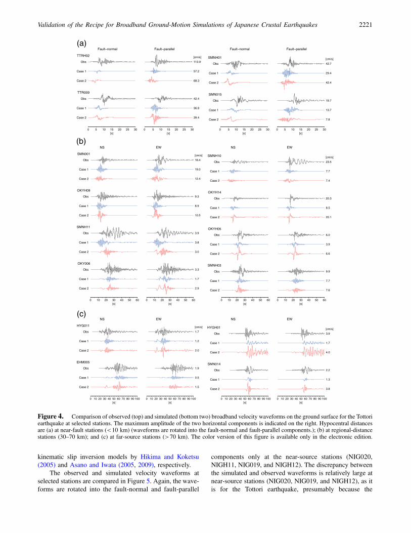
The observed and simulated broadband velocity wave-forms on the ground surface at selected stations are comparedin Figure 4. The x axis represents the lapse time from the oc-currence time by JMA, which corresponds to the starting timeof the simulations. The waveforms are rotated into the fault-normal and fault-parallel components only at the near-sourcestations (TTRH02, SMNH01, TTR009, and SMN015). Theamplitudes of the fault-normal components are noticeablyunderestimated by both cases at these stations. Iwata andSekiguchi (2002) simulated near-source ground motion usingtheir optimum source model, and discussed that the largeground velocity on the fault-normal component appears in theregion above and northwest of the hypocenter, which could beexplained by the upward and northwestward rupture propaga-tion with large rupture velocity. In this study, the rupture prop-agates at a constant rupture velocity starting from thehypocenter, which differs from the complicated rupture propa-gation pattern of the optimum model. Nevertheless, the am-plitudes of the fault-parallel component at SMNH01 andTTR009 are well represented by the simulations; this is likelyto be caused by the large stress drop at the southeast asperity(labeled as asperity 1 in Fig. 2a).
Strong pulses due to the rupture directivity observed atOKYH05 are also well represented by the simulations.However, the simulated waveforms do not explain the ob-served pulses at the near-source station TTRH02 where thehypocentral distance is smaller than 1 km. The observedwaveforms at SMN001 and SMNH10, which are locatednear the coast in the north of the source area, show relativelylong duration with later arrivals because of the velocitystructure. Such long-period dominant later phases are under-estimated by the simulations, which may reflect the insuffi-ciency of the 3D velocity structure model in this area.
2004 Chuetsu Earthquake
For the Chuetsu earthquake, we consider four cases:cases 1, 2, 3, and 4. The source parameters and fault configu-rations of the cases are shown in Table 3 and Figure 2b, re-spectively. The fault planes of the four cases are determinedby reference to the fault models by previous studies (Asanoand Iwata, 2005, 2009; Hikima and Koketsu, 2005). Theouter and inner fault parameters of cases 3 and 4 basicallyfollow the recipe, whereas some of the inner fault parametersof cases 1 and 2 follow the fault models by the previous stud-ies. The ratio of the area of asperity 1 (Sa1) to that of asperity2 (Sa2) is 2:1 for case 3 and 8:3 for case 4, and their locationsfollow the basic rule of the recipe. The locations of the asper-ities, the average slip Da, and the asperity area Sa of cases 1and 2 are obtained by modifying the recipe based on the
132º 133º 134º 135º
34º
35º
0 100
TTRH02
SMNH01
TTR009
SMN015
TTR007SMNH02
OKY015
OKYH07
OKYH10
SMNH11
OKYH08OKY006
HRS002
SMNH12
HRS021
OKY007
SMN001SMN001
SMN003
OKYH14
SMNH10SMNH10
OKYH09SMNH03
OKYH05
HRSH05
HYG004
SMN014
HYG011
OSKH01
EHM005
EHM001
HYG009
HYGH01
SMNH07
YMGH09
OSK001HYGH02
TKS011
SMN012
SMNH08
OKYH12
Seismic bedrock depth [km]
0.0 0.1 0.3 0.6 1.0 2.0 4.0 8.016.0
130º 140º
30º
40º
km
(a)
138º 139º 140º 141º
36º
37º
38º
0 100
NIG020NIGH11
NIG019
NIGH12
NIG021
NIGH06
NIGH10
NIG016
NIG015NIGH07
FKSH21
NIG023
NIG024
FKS028
NIGH15NIGH13
NIGH09
FKSH05
TCG003
TCGH17
FKS030
NIGH16
FKS026
NGNH07
GNM005
FKS029
GNMH09NGN004
NGNH29
YMT007
IBRH16
NGN018
SITH05
YMN006
FKSH12
GNMH10
FKSH08
FKS015
NIGH02
NGNH31
Seismic bedrock depth [km]
0.0 0.1 0.3 0.6 1.0 2.0 4.0 8.016.0
130º 140º
30º
40º
km
(b)
Figure 3. Study area for the (a) Tottori and (b) Chuetsu earth-quakes. The epicenter, stations, and the surface trace of the fault areindicated by a star, triangles, and a thick line, respectively. The scaleshows the depth of the seismic bedrock (VS ∼ 3000 m=s) of theJapan Seismic Hazard Information Station (J-SHIS) velocity struc-ture model. The color version of this figure is available only in theelectronic edition.
2220 A. Iwaki, T. Maeda, N. Morikawa, H. Miyake, and H. Fujiwara
kinematic slip inversion models by Hikima and Koketsu(2005) and Asano and Iwata (2005, 2009), respectively.
The observed and simulated velocity waveforms atselected stations are compared in Figure 5. Again, the wave-forms are rotated into the fault-normal and fault-parallel
components only at the near-source stations (NIG020,NIGH11, NIG019, and NIGH12). The discrepancy betweenthe simulated and observed waveforms is relatively large atnear-source stations (NIG020, NIG019, and NIGH12), as itis for the Tottori earthquake, presumably because the
(a)Fault−normal Fault−parallel Fault−normal Fault−parallel
TTRH02
Obs
Case 1
Case 2
113.9
57.2
68.3
[cm/s] SMNH01
Obs
Case 1
Case 2
42.7
29.4
42.4
[cm/s]
TTR009
Obs
Case 1
Case 2
42.4
36.8
39.4
SMN015
Obs
Case 1
Case 2
19.7
13.7
7.8
0 5 10 15 20 25 30[s]
0 5 10 15 20 25 30[s]
0 5 10 15 20 25 30[s]
0 5 10 15 20 25 30[s]
(b)NS EW NS EW
SMN001
Obs
Case 1
Case 2
16.4
19.0
12.4
[cm/s] SMNH10
Obs
Case 1
Case 2
23.5
7.7
7.4
[cm/s]
OKYH09
Obs
Case 1
Case 2
9.3
8.9
10.5
OKYH14
Obs
Case 1
Case 2
20.3
8.5
20.1
SMNH11
Obs
Case 1
Case 2
3.9
3.8
3.0
OKYH05
Obs
Case 1
Case 2
6.0
3.9
6.6
OKY006
Obs
Case 1
Case 2
3.3
1.7
2.9
SMNH03
Obs
Case 1
Case 2
9.9
7.7
7.6
0 10 20 30 40 50 60[s]
0 10 20 30 40 50 60[s] [s]
0 10 20 30 40 50 60 0 10 20 30 40 50 60[s]
(c)NS EW NS EW
HYG011
Obs
Case 1
Case 2
1.7
1.2
2.0
[cm/s] HYGH01
Obs
Case 1
Case 2
3.9
1.7
4.0
[cm/s]
EHM005
Obs
Case 1
Case 2
1.9
0.5
1.5
SMN014
Obs
Case 1
Case 2
2.2
1.3
3.8
0 10 20 30 40 50 60 70 80 90 100[s]
0 10 20 30 40 50 60 70 80 90 100[s]
0 10 20 30 40 50 60 70 80 90 100[s]
0 10 20 30 40 50 60 70 80 90 100[s]
Figure 4. Comparison of observed (top) and simulated (bottom two) broadband velocity waveforms on the ground surface for the Tottoriearthquake at selected stations. The maximum amplitude of the two horizontal components is indicated on the right. Hypocentral distancesare (a) at near-fault stations (<10 km) (waveforms are rotated into the fault-normal and fault-parallel components.); (b) at regional-distancestations (30–70 km); and (c) at far-source stations (>70 km). The color version of this figure is available only in the electronic edition.
Validation of the Recipe for Broadband Ground-Motion Simulations of Japanese Crustal Earthquakes 2221

(a)Fault−normal Fault−parallel Fault−normal Fault−parallel
NIG020
Obs
Case 1
Case 2
Case 3
Case 4
37.7
32.2
44.6
45.8
46.3
[cm/s] NIGH11
Obs
Case 1
Case 2
Case 3
Case 4
64.6
37.1
34.6
33.6
34.2
[cm/s]
NIG019
Obs
Case 1
Case 2
Case 3
Case 4
128.2
56.9
49.3
73.8
61.7
NIGH12
Obs
Case 1
Case 2
Case 3
Case 4
28.5
15.7
19.6
26.8
26.5
0 5 10 15 20 25 30[s]
0 5 10 15 20 25 30[s]
0 5 10 15 20 25 30[s]
0 5 10 15 20 25 30[s]
(b)NS EW NS EW
NIG023
Obs
Case 1
Case 2
Case 3
Case 4
27.7
12.4
13.4
11.8
13.5
[cm/s] FKS028
Obs
Case 1
Case 2
Case 3
Case 4
11.8
10.0
10.0
7.0
6.3
[cm/s]
NIGH13
Obs
Case 1
Case 2
Case 3
Case 4
5.4
3.1
2.7
3.0
3.3
NIGH07
Obs
Case 1
Case 2
Case 3
Case 4
3.5
5.2
3.7
3.2
3.8
FKS030
Obs
Case 1
Case 2
Case 3
Case 4
5.9
6.9
4.7
4.2
4.0
NGNH07
Obs
Case 1
Case 2
Case 3
Case 4
3.1
2.0
3.0
2.2
2.2
0 10 20 30 40 50 60[s]
0 10 20 30 40 50 06[s]
0 10 20 30 40 50 60[s]
0 10 20 30 40 50 60[s]
(c)NS EW NS EW
GNM005
Obs
Case 1
Case 2
Case 3
Case 4
2.6
1.5
1.9
1.6
1.8
[cm/s] NGN004
Obs
Case 1
Case 2
Case 3
Case 4
1.9
1.1
1.4
1.2
1.2
[cm/s]
FKSH08
Obs
Case 1
Case 2
Case 3
Case 4
1.0
1.1
1.2
1.1
1.2
YMN006
Obs
Case 1
Case 2
Case 3
Case 4
0.5
0.3
0.3
0.3
0.4
0 10 20 30 40 50 60 70 80 90 100[s]
0 10 20 30 40 50 60 70 80 90 100[s]
0 10 20 30 40 50 60 70 80 90 100[s]
0 10 20 30 40 50 60 70 80 90 100[s]
Figure 5. Comparison of observed (top) and simulated (bottom two) broadband velocity waveforms on the ground surface for the Chuetsuearthquake at selected stations. The maximum amplitude of the two horizontal components is indicated on the right. Hypocentral distancesare (a) at near-fault stations (<10 km) (waveforms are rotated into the fault-normal and fault-parallel components.); (b) at regional-distancestations (30–70 km); and (c) at far-source stations (>70 km). The color version of this figure is available only in the electronic edition.
2222 A. Iwaki, T. Maeda, N. Morikawa, H. Miyake, and H. Fujiwara

simulation results at near-source stations are directly affectedby the source parameters. As the source region of theChuetsu earthquake is located on deep sedimentary layers,the waveforms are particularly complicated because of thecombination of the fault rupture and the wave propagationeffects, but they are generally well reproduced by the simu-lations at regional and far-source stations. For example, theobserved waveforms at NIGH13 show not only large pulsesfrom the source with short duration but also later arrivalsfrom the surface wave, which is reproduced by the simula-tions. The simulated waveforms overestimate the surfacewaves at NGNH07, suggesting the need for improvementof the velocity structure model in this area.
Broadband Ground-Motion Validation
Peak Ground Velocity and Seismic Intensity
PGVand IJMA, as well as the velocity waveforms, are theground-motion indexes that have been conventionally usedto validate the recipe (e.g., Fujiwara, Kawai, Aoi, Morikawa,
Senna, Kudo, Ooi, Hao, Wakamatsu, et al., 2009). Theobserved and simulated PGVs for the Tottori and Chuetsuearthquakes are compared in Figures 6 and 7, respectively.The overall spatial distribution of PGV is explained by thesimulations, except for case 2 of the Tottori earthquake inwhich the simulated PGV at some regional- and far-sourcestations overestimates the observation. It should be noted thatPGVs in Figures 6 and 7 may differ from the maximum am-plitudes of the velocity waveforms in Figures 4 and 5, reflect-ing the difference between the two methods (left and rightsides of Fig. 1a) for modeling the near-surface site effects.
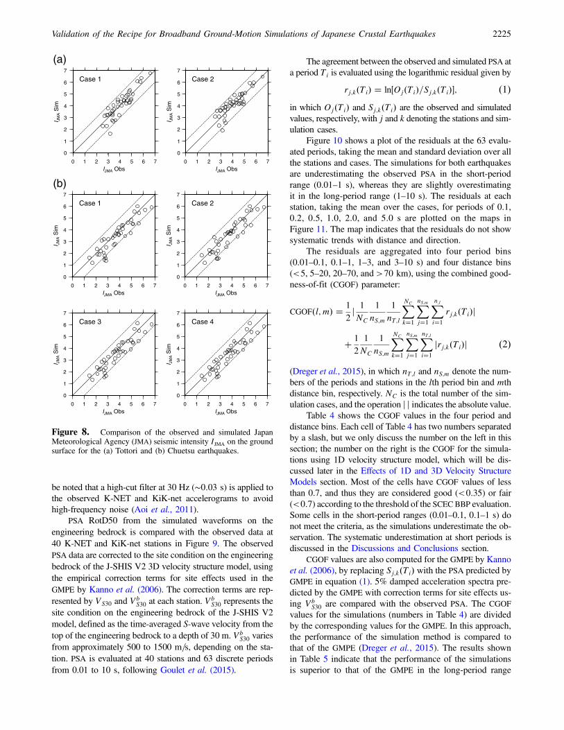
The observed and simulated IJMA values are compared inFigure 8. The observed IJMA is computed from the time seriesof the observed records. The simulated IJMA generally showsa good agreement with the observed values for both earth-quakes. However, the largest observed IJMA of 7 at NIG019for the Chuetsu earthquake was not reproduced by the simu-lations. Because IJMA is calculated from acceleration wave-forms, short-period components of ground motion may haveplayed a large role in such underestimation of IJMA.
132º 133º 134º 135º
34º
35º
Obs.
132º 133º 134º 135º
34º
35º
Case 1
132º 133º 134º 135º
34º
35º
Case 2
0
5
10
20
30
40
60
80
120PGV [cm/s]
100
101
102
PG
V S
im [c
m/s
]
100 101 102
PGV Obs [cm/s]
Case 1
100
101
102
PG
V S
im [c
m/s
]
100 101 102
PGV Obs [cm/s]
Case 2
Figure 6. Observed and simulated (cases 1 and 2) peak ground velocities (PGVs) on the ground surface plotted on the map for the Tottoriearthquakes. The stars represent the epicenters. The bottom panels compare the observed and simulated PGVs.
Validation of the Recipe for Broadband Ground-Motion Simulations of Japanese Crustal Earthquakes 2223
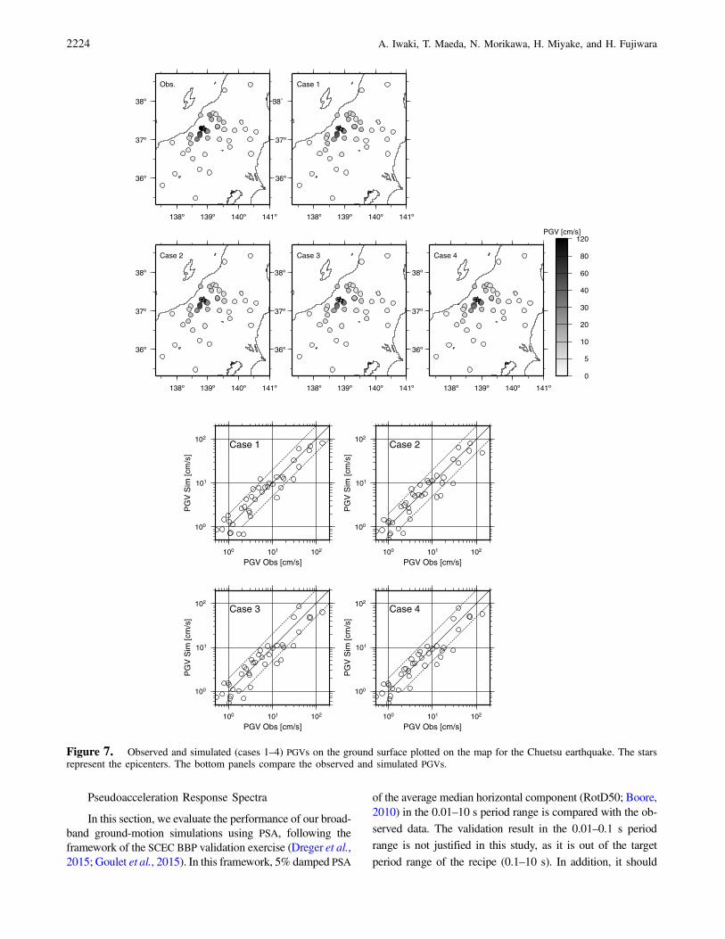
Pseudoacceleration Response Spectra
In this section, we evaluate the performance of our broad-band ground-motion simulations using PSA, following theframework of the SCEC BBP validation exercise (Dreger et al.,2015; Goulet et al., 2015). In this framework, 5% damped PSA
of the average median horizontal component (RotD50; Boore,2010) in the 0.01–10 s period range is compared with the ob-served data. The validation result in the 0.01–0.1 s periodrange is not justified in this study, as it is out of the targetperiod range of the recipe (0.1–10 s). In addition, it should
138º 139º 140º 141º
36º
37º
38º
Obs.
138º 139º 140º 141º
36º
37º
38˚
Case 1
138º 139º 140º 141º
36º
37º
38º
Case 2
138º 139º 140º 141º
36º
37º
38º
Case 3
138º 139º 140º 141º
36º
37º
38º
Case 4
0
5
10
20
30
40
60
80
120PGV [cm/s]
100
101
102
PG
V S
im [c
m/s
]
100 101 102
PGV Obs [cm/s]
Case 1
100
101
102
PG
V S
im [c
m/s
]
100 101 102
PGV Obs [cm/s]
Case 2
100
101
102
PG
V S
im [c
m/s
]
100 101 102
PGV Obs [cm/s]
Case 3
100
101
102
PG
V S
im [c
m/s
]
100 101 102
PGV Obs [cm/s]
Case 4
Figure 7. Observed and simulated (cases 1–4) PGVs on the ground surface plotted on the map for the Chuetsu earthquake. The starsrepresent the epicenters. The bottom panels compare the observed and simulated PGVs.
2224 A. Iwaki, T. Maeda, N. Morikawa, H. Miyake, and H. Fujiwara
be noted that a high-cut filter at 30 Hz (∼0:03 s) is applied tothe observed K-NET and KiK-net accelerograms to avoidhigh-frequency noise (Aoi et al., 2011).
PSA RotD50 from the simulated waveforms on theengineering bedrock is compared with the observed data at40 K-NET and KiK-net stations in Figure 9. The observedPSA data are corrected to the site condition on the engineeringbedrock of the J-SHIS V2 3D velocity structure model, usingthe empirical correction terms for site effects used in theGMPE by Kanno et al. (2006). The correction terms are rep-resented by VS30 and Vb
S30 at each station. VbS30 represents the
site condition on the engineering bedrock of the J-SHIS V2model, defined as the time-averaged S-wave velocity from thetop of the engineering bedrock to a depth of 30 m. Vb
S30 variesfrom approximately 500 to 1500 m=s, depending on the sta-tion. PSA is evaluated at 40 stations and 63 discrete periodsfrom 0.01 to 10 s, following Goulet et al. (2015).
The agreement between the observed and simulated PSA ata period Ti is evaluated using the logarithmic residual given by
EQ-TARGET;temp:intralink-;df1;313;709rj;k�Ti� � ln�Oj�Ti�=Sj;k�Ti��; �1�in which Oj�Ti� and Sj;k�Ti� are the observed and simulatedvalues, respectively, with j and k denoting the stations and sim-ulation cases.
Figure 10 shows a plot of the residuals at the 63 evalu-ated periods, taking the mean and standard deviation over allthe stations and cases. The simulations for both earthquakesare underestimating the observed PSA in the short-periodrange (0.01–1 s), whereas they are slightly overestimatingit in the long-period range (1–10 s). The residuals at eachstation, taking the mean over the cases, for periods of 0.1,0.2, 0.5, 1.0, 2.0, and 5.0 s are plotted on the maps inFigure 11. The map indicates that the residuals do not showsystematic trends with distance and direction.
The residuals are aggregated into four period bins(0.01–0.1, 0.1–1, 1–3, and 3–10 s) and four distance bins(<5, 5–20, 20–70, and >70 km), using the combined good-ness-of-fit (CGOF) parameter:EQ-TARGET;temp:intralink-;df2;313;481
CGOF�l; m� � 1
2j 1
NC
1
nS;m
1
nT;l
XNC
k�1
XnS;m
j�1
Xn;l
i�1
rj;k�Ti�j
� 1
2
1
NC
1
nS;m
XNC
k�1
XnS;m
j�1
XnT;l
i�1
jrj;k�Ti�j �2�
(Dreger et al., 2015), in which nT;l and nS;m denote the num-bers of the periods and stations in the lth period bin and mthdistance bin, respectively. NC is the total number of the sim-ulation cases, and the operation j j indicates the absolute value.
Table 4 shows the CGOF values in the four period anddistance bins. Each cell of Table 4 has two numbers separatedby a slash, but we only discuss the number on the left in thissection; the number on the right is the CGOF for the simula-tions using 1D velocity structure model, which will be dis-cussed later in the Effects of 1D and 3D Velocity StructureModels section. Most of the cells have CGOF values of lessthan 0.7, and thus they are considered good (<0:35) or fair(<0:7) according to the threshold of the SCEC BBP evaluation.Some cells in the short-period ranges (0.01–0.1, 0.1–1 s) donot meet the criteria, as the simulations underestimate the ob-servation. The systematic underestimation at short periods isdiscussed in the Discussions and Conclusions section.
CGOF values are also computed for the GMPE by Kannoet al. (2006), by replacing Sj;k�Ti� with the PSA predicted byGMPE in equation (1). 5% damped acceleration spectra pre-dicted by the GMPE with correction terms for site effects us-ing Vb
S30 are compared with the observed PSA. The CGOFvalues for the simulations (numbers in Table 4) are dividedby the corresponding values for the GMPE. In this approach,the performance of the simulation method is compared tothat of the GMPE (Dreger et al., 2015). The results shownin Table 5 indicate that the performance of the simulationsis superior to that of the GMPE in the long-period range
0
1
2
3
4
5
6
7
I JM
A S
im
0 1 2 3 4 5 6 7IJMA Obs
(a)
Case 1
0
1
2
3
4
5
6
7
I JM
A S
im0 1 2 3 4 5 6 7
IJMA Obs
Case 2
0
1
2
3
4
5
6
7
I JM
A S
im
0 1 2 3 4 5 6 7IJMA Obs
Case 1
0
1
2
3
4
5
6
7
I JM
A S
im
0 1 2 3 4 5 6 7IJMA Obs
Case 2
0
1
2
3
4
5
6
7
I JM
A S
im
0 1 2 3 4 5 6 7IJMA Obs
Case 3
0
1
2
3
4
5
6
7
I JM
A S
im
0 1 2 3 4 5 6 7IJMA Obs
Case 4
(b)
Figure 8. Comparison of the observed and simulated JapanMeteorological Agency (JMA) seismic intensity IJMA on the groundsurface for the (a) Tottori and (b) Chuetsu earthquakes.
Validation of the Recipe for Broadband Ground-Motion Simulations of Japanese Crustal Earthquakes 2225

(3–10 s), whereas many cells in the shorter-period ranges areindicated as being comparable to or inferior to the GMPE.
We recognize that the values in Tables 4 and 5 shouldnot be directly compared with those of the SCEC BBP val-idation results shown in Dreger et al. (2015) for two majorreasons: the first is that we assumed that the approximate
locations of the asperities are known prior to modelingthe source, and the second is that we used a well-calibrated3D velocity structure model. The latter will be discussed in alater section, by performing the broadband ground-motionsimulation using the same 1D velocity structure as in theSCEC BBP validation. However, the current results demon-strate the performance of the recipe including the character-ized source model and the 3D velocity structure model.
Effects of 1D and 3D Velocity Structure Models
As mentioned in the previous section, the velocity struc-ture model used in this study is different from that used in theSCEC BBP validation. In the SCEC BBP validation, 1D lay-ered velocity structure models for western and central Japanby Goulet et al. (2015) are used for the Tottori and Chuetsuearthquakes, respectively (hereafter referred as 1D velocitystructure model). We perform broadband ground-motion simu-lations using the 1D velocity structure models (1D simulations)with the same source models in the simulations discussed earlier(3D simulations) to validate the performance of PSA RotD50.We use the corrected PSA data by Goulet et al. (2015), whichare adjusted to a site condition with VS30 of 863 m=s, whichcorresponds to Vb
S30 of the 1D velocity structure models.The numbers on the right of the slashes in Table 4 are
the CGOF values obtained from the 1D simulations, andFigure 12 shows a plot of the residuals. 94% and 85% of thecells in Table 4 are found to meet the criterion (CGOF < 0:7)for the Tottori and Chuetsu earthquakes, respectively, which
(a)Obs Case 1
Case 2
TTRH02
10−3
10−2
10−1
100
PS
A [g
]
10−2 10−1 100 101
SMNH01
10−3
10−2
10−1
100
10−2 10−1 100 101
TTR009
10−3
10−2
10−1
100
10−2 10−1 100 101
SMN015
10−3
10−2
10−1
100
10−2 10−1 100 101
SMN001
10−3
10−2
10−1
100
PS
A [g
]
10−2 10−1 100 101
SMNH10
10−3
10−2
10−1
100
10−2 10−1 100 101
OKYH09
10−3
10−2
10−1
100
10−2 10−1 100 101
OKYH14
10−3
10−2
10−1
100
10−2 10−1 100 101
SMNH11
10−3
10−2
10−1
100
PS
A [g
]
10−2 10−1 100 101
OKYH05
10−3
10−2
10−1
100
10−2 10−1 100 101
OKY006
10−3
10−2
10−1
100
10−2 10−1 100 101
SMNH03
10−3
10−2
10−1
100
10−2 10−1 100 101
HYG011
10−3
10−2
10−1
100
PS
A [g
]
10−2 10−1 100 101
Period [s]
HYGH01
10−3
10−2
10−1
100
10−2 10−1 100 101
Period [s]
EHM005
10−3
10−2
10−1
100
10−2 10−1 100 101
Period [s]
SMN014
10−3
10−2
10−1
100
10−2 10−1 100 101
Period [s]
(b) Obs Case 1
Case 2
Case 3
Case 4
NIG020
10−3
10−2
10−1
100
PS
A [g
]
10−2 10−1 100 101
NIGH11
10−3
10−2
10−1
100
10−2 10−1 100 101
NIG019
10−3
10−2
10−1
100
10−2 10−1 100 101
NIGH12
10−3
10−2
10−1
100
10−2 10−1 100 101
NIG023
10−3
10−2
10−1
100
PS
A [g
]
10−2 10−1 100 101
FKS028
10−3
10−2
10−1
100
10−2 10−1 100 101
NIGH10
10−3
10−2
10−1
100
10−2 10−1 100 101
NIGH13
10−3
10−2
10−1
100
10−2 10−1 100 101
NIG015
10−3
10−2
10−1
100
PS
A [g
]
10−2 10−1 100 101
NIGH07
10−3
10−2
10−1
100
10−2 10−1 100 101
FKS030
10−3
10−2
10−1
100
10−2 10−1 100 101
NGNH07
10−3
10−2
10−1
100
10−2 10−1 100 101
GNM005
10−3
10−2
10−1
100
PS
A [g
]10−2 10−1 100 101
Period [s]
NGN004
10−3
10−2
10−1
100
10−2 10−1 100 101
Period [s]
FKSH08
10−3
10−2
10−1
100
10−2 10−1 100 101
Period [s]
YMN006
10−3
10−2
10−1
100
10−2 10−1 100 101
Period [s]
Figure 9. 5% damped PSA RotD50 for the (a) Tottori and (b) Chuetsu earthquakes. The thick lines correspond to the observed datacorrected to the site condition of the engineering bedrock. Simulated PSA are plotted by different lines given in the legend. The color versionof this figure is available only in the electronic edition.
−2.0−1.5−1.0−0.5
0.00.51.01.52.0
ln(o
bs/s
im)
0.01 0.1 1 10
Period [s]
(a)Tottori 3D
−2.0−1.5−1.0−0.5
0.00.51.01.52.0
ln(o
bs/s
im)
0.01 0.1 1 10
Period [s]
(b)Chuetsu 3D
Figure 10. Plot of PSA residuals (see equation 1) with a period0.01–10 s for the (a) Tottori and (b) Chuetsu earthquakes. The meanand standard deviation for all stations and cases are shown by solidand dashed lines, respectively.
2226 A. Iwaki, T. Maeda, N. Morikawa, H. Miyake, and H. Fujiwara

is considered acceptable because the cells that fail the cri-terion are in the 0.01–0.1 s period range. In the shorter-periodranges (<1 s), the CGOF values for the 1D simulations areslightly better than the 3D simulations (numbers on the left inTable 4). On the other hand, the 3D simulations performedbetter in the longer-period ranges (>1 s), especially for theChuetsu earthquake.
Figures 13 and 14 show PSA RotD50 and broadbandvelocity waveforms, respectively, obtained from the 1Dand 3D simulations, at stations located on deep sedimentarylayers. Only case 3 of the Chuetsu earthquake is shown as anexample. The difference between PSA of 1D and 3D simu-lations is especially large at long periods (>1 s). Waveformsfrom the 3D simulation have later phases with larger ampli-
132º 133º 134º 135º
34º
35º
Period = 0.100 s
132º 133º 134º 135º
34º
35º
Period = 0.200 s
132º 133º 134º 135º
34º
35º
Period = 0.500 s
132º 133º 134º 135º
34º
35º
Period = 1.000 s
132º 133º 134º 135º
34º
35º
Period = 2.000 s
132º 133º 134º 135º
34º
35º
Period = 5.000 s
−1.5
−1.2
−0.9
−0.6
−0.3
0.0
0.3
0.6
0.9
1.2
1.5
138º 139º 140º 141º
36º
37º
38º
Period = 0.100 s
138º 139º 140º 141º
36º
37º
38º
Period = 0.200 s
138º 139º 140º 141º
36º
37º
38º
Period = 0.500 s
138º 139º 140º 141º
36º
37º
38º
Period = 1.000 s
138º 139º 140º 141º
36º
37º
38º
Period = 2.000 s
138º 139º 140º 141º
36º
37º
38º
Period = 5.000 s
−1.5
−1.2
−0.9
−0.6
−0.3
0.0
0.3
0.6
0.9
1.2
1.5
(a)
(b)
Figure 11. PSA residuals on a map at periods 0.1, 0.2, 0.5, 1.0, 2.0, and 5.0 s for the (a) Tottori and (b) Chuetsu earthquakes. Positive andnegative values are plotted by circles and squares, respectively. The stars represent the epicenters.
Validation of the Recipe for Broadband Ground-Motion Simulations of Japanese Crustal Earthquakes 2227

tudes and longer durations and show better agreement withthe observation. The differences between the 1D and 3Dvelocity structure models beneath the stations are shownin Figure 15. The observed later phases with long-periodcomponents at these stations are underestimated by the1D simulation; this can be attributed to the lack of deepsediment with spatially dependent depth that varies from1 to 8 km. The results suggest the importance of using3D velocity structure models to obtain realistic ground-motion predictions.
Discussion and Conclusions
We performed a validation of the broadband ground-mo-tion method called the recipe for the Tottori and Chuetsuearthquakes (Mw 6.6) using velocity waveforms, PGV, IJMA,and 5% damped PSA of the RotD50 component. The simu-lated velocity waveforms well reproduced the characteristicsof the observed waveforms, including the near-fault pulsesand later arrival phases with relatively long-period compo-nents. However, the simulated waveforms did not matchwell with the observation particularly at near-source stations.At near-source stations, the simulation results are mostlyaffected by the source models. It should be noted that ourgoal is not to perfectly reproduce the observed waveforms
Table 4The Combined Goodness-of-fit (CGOF) for the BroadbandGround-Motion Simulations with the 3D and 1D Velocity
Structure Models
PSA Period/Distance(km) 0.01–0.1 s 0.1–1 s 1–3 s 3–10 s
Numberof
Stations*
Tottori<5 0.29/0.32 0.63/0.31 0.17/0.38 0.15/0.28 15–20 0.38/0.25 0.29/0.26 0.45/0.41 0.45/0.29 720–70 0.97/0.70 0.33/0.34 0.46/0.56 0.39/0.57 16>70 1.09/0.88 0.71/0.65 0.59/0.58 0.34/0.58 16
Chuetsu<5 05–20 0.82/0.60 0.45/0.41 0.45/0.53 0.17/0.39 520–70 1.03/0.72 0.55/0.41 0.32/0.41 0.25/0.35 18>70 1.33/1.00 0.68/0.53 0.53/0.41 0.35/0.37 17
In each cell, the numbers on the left and right sides of the slash denote theCGOFs for 3D and 1D velocity structure models, respectively. The bold,regular, and italic fonts indicate good (<0:35), fair (<0:7), and poor (>0:7)thresholds, respectively, following the Southern California EarthquakeCenter (SCEC) Broadband Platform (BBP) validation (Dreger et al., 2015).PSA, pseudoacceleration response spectra.*The number of stations that are included in the corresponding distance bins.
There is no station within 5 km from the hypocenter for Chuetsu earthquake.
Table 5Ratio of CGOF for the Broadband Ground-MotionSimulations and the Ground-Motion Prediction
Equation (GMPE)
PSA Period/Distance (km)
0.01–0.1 s 0.1–1 s 1–3 s 3–10 s Number ofStations
Tottori<5 0.19 0.70 0.16 0.14 15–20 0.75 1.04 2.20 0.96 720–70 2.36 1.02 1.26 0.78 16>70 2.12 1.23 1.55 0.87 16
Chuetsu<5 05–20 2.72 0.87 1.29 0.25 520–70 4.07 1.59 1.02 0.34 18>70 2.89 1.49 0.87 0.50 17
The CGOF numbers for 3D simulations in Table 4 are divided by thecorresponding numbers for the GMPE. Bold, regular, and italic fontsindicate better than GMPE (<1:0), comparable to GMPE (<1:5), andinferior to GMPE (>1:5) thresholds, respectively, following Dregeret al. (2015).
−2.0−1.5−1.0−0.5
0.00.51.01.52.0
ln(o
bs/s
im)
0.01 0.1 1 10
Period [s]
(a)Tottori 1D
−2.0−1.5−1.0−0.5
0.00.51.01.52.0
ln(o
bs/s
im)
0.01 0.1 1 10Period [s]
(b)Chuetsu 1D
Figure 12. Plot of the PSA residuals for the 1D simulations forthe (a) Tottori and (b) Chuetsu earthquakes. The mean and standarddeviation of all stations and cases are shown by solid and dashedlines, respectively.
Obs Case 3 3D
Case 3 1D
NIGH11
10−3
10−2
10−1
100
PS
A [g
]
10−2 10−1 100 101
NIG021
10−3
10−2
10−1
100
10−2 10−1 100 101
NIG023
10−3
10−2
10−1
100
10−2 10−1 100 101
GNM005
10−3
10−2
10−1
100
PS
A [g
]
10−2 10−1 100 101
Period [s]
NGN004
10−3
10−2
10−1
100
10−2 10−1 100 101
Period [s]
YMN006
10−3
10−2
10−1
100
10−2 10−1 100 101
Period [s]
Figure 13. Comparison of 5% damped PSA RotD50 from thecase 3 simulation of the Chuetsu earthquake using the 3D (thinlines) and 1D (dashed lines) velocity structure models. The thicktraces correspond to the observed data corrected to a site conditionwith VS30 of 863 m=s.
2228 A. Iwaki, T. Maeda, N. Morikawa, H. Miyake, and H. Fujiwara

NS EW NS EW
NIGH11
Obs
3D
1D
55.9
29.1
14.7
[cm/s] NIG021
Obs
3D
1D
58.0
18.3
12.8
[cm/s]
NIG023
Obs
3D
1D
27.7
11.8
4.6
GNM005
Obs
3D
1D
2.6
1.6
0.8
NGN004
Obs
3D
1D
1.9
1.2
0.9
YMN006
Obs
3D
1D
0.5
0.3
0.2
0 10 20 30 40 50 60 70 80 90 100
[s]
0 10 20 30 40 50 60 70 80 90 100
[s]
0 10 20 30 40 50 60 70 80 90 100
[s]
0 10 20 30 40 50 60 70 80 90 100
[s]
Figure 14. Comparison of the broadband velocity waveforms on the ground surface for the simulations using the 3D (case 3) and 1Dvelocity structure models for the Chuetsu earthquake. The top lines represent the observed data.
0
5
10
Dep
th [k
m]
0 1 2 3 4
VS [km/s]
NIGH11
0
5
10
Dep
th [k
m]
0 1 2 3 4
VS [km/s]
NIG021
0
5
10
Dep
th [k
m]
0 1 2 3 4
VS [km/s]
NIG023
3D
1D
0
5
10
Dep
th [k
m]
0 1 2 3 4
VS [km/s]
GNM005
0
5
10
Dep
th [k
m]
0 1 2 3 4
VS [km/s]
NGN004
0
5
10
Dep
th [k
m]
0 1 2 3 4
VS [km/s]
YMN006
Figure 15. VS structures extracted from the 3D (solid lines) and 1D (dashed lines) velocity structure models at selected sites for theChuetsu earthquake.
Validation of the Recipe for Broadband Ground-Motion Simulations of Japanese Crustal Earthquakes 2229

because the goal of this study is to validate the recipe as atool for predicting ground motion under conditions that thesource parameters are poorly constrained. The simulationsalso underestimated the later phases at some stations, sug-gesting the insufficiency of the 3D velocity structure model.When the velocity structure model is further improvedin the future, the simulation results are also expected to beimproved.
The simulated PGV and IJMA generally agreed well withthe observation, except for IJMA for the Chuetsu earthquake atthe nearest-fault station NIG019, where the simulationsunderestimated the observed IJMA of 7. We followed the pro-cedure of the SCEC BBP validation presented by Dreger et al.(2015) for the validation using PSA RotD50 and demon-strated that the performance of our simulations is generallyacceptable. We found that the performance could be deemedpoor in the short-period ranges (0.01–0.1 and 0.1–1 s) atlarge hypocentral distance (>70 km). It should be noted thatthe recipe has not been validated for the shortest-period rangeof 0.01–0.1 s so far; therefore, the results in this period rangeare not justified in this study.
There are at least two factors that may have caused thesystematic underestimation in the short-period ranges. Thefirst is the choice of fmax, the frequency at which an acceler-ation spectrum begins to fall off at high frequencies (Hanks,1982). Currently, fmax is set at 6 Hz for all crustal earthquakesin Japan in the scenario earthquake shaking maps. Becausefmax controls the amplitude of high-frequency ground motion,further investigation may be needed to determine appropriateregional values of fmax. The second factor is the deep subsur-face velocity structure model. As shown in Figure 9a, the sim-ulations largely underestimated the observed PSA for periodsin the 0.01–1 s range at some stations such as OKY006,OKYH14, and HYG011, most of which are in a mountainousarea where Vb
S30 is approximately 1200–1500 m=s. It is pos-sible that the short-period (<1 s) components of the groundmotion are not appropriately generated on the engineeringbedrock. Improvement on the deep subsurface structure modelis in progress (e.g., Senna et al., 2013), considering the weath-ered layer on the bedrock and the interaction between the shal-low and deep subsurface structure.
We also conducted ground-motion simulations using the1D velocity structure models used in SCEC BBP validationand compared the results with those obtained from the sim-ulations using the 3D velocity structure model. We found thatCGOF values for the 3D simulations were better than thosefor the 1D simulations at periods longer than 1 s. In addition,the time series of velocity waveforms from the two types ofsimulations significantly differed from each other. The veloc-ity waveforms from the 3D simulation show better agreementwith the observation, especially in reproducing the large laterphases and long durations observed at deep sediment sites,which demonstrated the importance of using 3D velocitystructure models in ground-motion prediction. Moreover,it is suggested that the characteristics of the ground motionshould be evaluated not only by response spectra but also by
some features of the time series waveforms, as shown byPaolucci et al. (2015). Therefore, future work should concen-trate on quantitative evaluation of waveforms, which is nec-essary for more comprehensive validation of broadbandground-motion prediction methods.
Data and Resources
The ground-motion data and the logging data were ob-tained from the National Research Institute for Earth Scienceand Disaster Prevention (NIED) strong-motion seismographnetworks K-NET and KiK-net (http://www.kyoshin.bosai.go.jp, last accessed May 2016; Aoi et al., 2011). The NationalSeismic Hazard Maps for Japan, the long-term evaluation ofthe active faults, and the recipe were documented by the Earth-quake Research Committee (ERC) of the Headquarters ofEarthquake Research Promotion (HERP) of Japan (http://www.jishin.go.jp/main/index-e.html, last accessed May 2016).The National Seismic Hazard Maps for Japan, the long-termevaluation of the active faults, and the Japan Seismic HazardInformation Station v.2 (J-SHIS V2) 3D velocity structuremodel can also be accessed online (http://www.j-shis.bosai.go.jp/en/, last accessedMay 2016). Most figures were drawnusing the Generic Mapping Tools v.4.5.8 (http://www.soest.hawaii.edu/gmt, last accessed May 2016; Wessel andSmith, 1998).
Acknowledgments
We thank the Earthquake Research Committee (ERC) of the Head-quarters of Earthquake Research Promotion (HERP) of Japan, as well as Ka-zuki Koketsu, James Mori, Kojiro Irikura, Hiroshi Kawase, Paul Somerville,Arben Pitarka, Christine Goulet, Phil Maechling, Fabio Silva, and NormAbrahamson for their helpful suggestions and discussions. Insightful com-ments from two anonymous reviewers and Associate Editor Luis A.Dalguer are greatly appreciated.
References
Aoi, S., and H. Fujiwara (1999). 3D finite-difference method using discon-tinuous grids, Bull. Seismol. Soc. Am. 89, 918–930.
Aoi, S., T. Hayakawa, and H. Fujiwara (2004). Ground Motion Simulator:GMS, BUTSURI-TANSA 57, 651–666 (in Japanese with Englishabstract).
Aoi, S., T. Kunugi, H. Nakamura, and H. Fujiwara (2011). Deployment ofnew strong motion seismographs of K-NETand KiK-net, in EarthquakeData in Engineering Seismology: Predictive Models, Data Managementand Networks, Geotechnical, Geological, and Earthquake Engineering,S. Akkar, P. Gülkan, and T. van Eck (Editors), Vol. 14, Springer,Dordrecht, The Netherlands, 167–186.
Asano, K., and T. Iwata (2005). Source rupture models of recent disastrousearthquakes in Japan, APRU/AEARU Research Symposium 2005,Kyoto, Japan, P08.
Asano, K., and T. Iwata (2009). Source rupture process of the 2004 Chuetsu,mid-Niigata prefecture, Japan, earthquake inferred from waveforminversion with dense strong-motion data, Bull. Seismol. Soc. Am. 99,123–140.
Baker, J. W. (2007). Quantitative classification of near-fault ground motionsusing wavelet analysis, Bull. Seismol. Soc. Am. 97, 1486–1501.
Bertero, V. V., S. A. Mahin, and R. A. Herrera (1978). Aseismic designimplications of near-fault San Fernando earthquake records, Earthq.Eng. Struct. Dynam. 6, 31–42.
2230 A. Iwaki, T. Maeda, N. Morikawa, H. Miyake, and H. Fujiwara

Boore, D. M. (1983). Stochastic simulation of high-frequency groundmotions based on seismological models of the radiated spectra, Bull.Seismol. Soc. Am. 73, 1865–1894.
Boore, D. M. (2010). Orientation-independent, nongeometric-mean mea-sures of seismic intensity from two horizontal components of motion,Bull. Seismol. Soc. Am. 100, 1830–1835.
Boore, D. M., C. D. Alessandro, and N. A. Abrahamson (2014). A gener-alization of the double-corner-frequency source spectral model and itsuse in the SCEC BBP validation exercise, Bull. Seismol. Soc. Am. 104,2387–2398.
Dan, K., and T. Sato (1998). Strong-motion prediction by semi-empiricalmethod based on variable-slip rupture model of earthquake fault, J.Arch. Inst. Japan 509, 49–60 (in Japanese with English abstract).
Dan, K., M. Watanabe, T. Sato, and T. Ishii (2001). Short-period sourcespectra inferred from variable-slip rupture models and modeling ofearthquake fault for strong motion prediction, J. Arch. Inst. Japan545, 51–62 (in Japanese with English abstract).
Das, S., and B. V. Kostrov (1986). Fracture of a single asperity on a finitefault: A model for weak earthquakes? in Earthquake Source Mechan-ics, S. Das, J. Boatwright, and C. H. Scholz (Editors), American Geo-physical Monograph, Vol. 37, 91–96.
Dreger, D. S., G. C. Beroza, S. M. Day, C. A. Goulet, T. H. Jordan, P. A.Spudich, and J. P. Stewart (2015). Validation of the SCEC broadbandplatform V14.3 simulation methods using pseudospectral accelerationdata, Seismol. Res. Lett. 86, 39–47.
Earthquake Research Committee (ERC) (2005). Report: National SeismicHazard Maps for Japan, http://www.jishin.go.jp/main/chousa/06mar_yosoku‑e/NationalSeismicHazardMaps.pdf (last accessed October2015).
Earthquake Research Committee (ERC) (2009). Strong Motion PredictionMethod (“Recipe”) for Earthquake with Specified Source Faults, http://jishin.go.jp/main/chousa/09_yosokuchizu/g_furoku3.pdf (last ac-cessed October 2015) (in Japanese).
Fujimoto, K., and S. Midorikawa (2006). Relationship between averageshear-wave velocity and site amplification inferred from strong motionrecords at nearby station pairs, J. Japan Assoc. Earthq. Eng. 6, no. 1,11–22 (in Japanese with English abstract).
Fujiwara, H., S. Kawai, S. Aoi, N. Morikawa, S. Senna, N. Kudo, M. Ooi,K. X.-S. Hao, Y. Hayakawa, N. Toyama, et al. (2009). A study onsubsurface structure model for deep sedimentary layers of Japanfor strong-motion evaluation, Technical Note of the National Res.Inst. for Earth Science and Disaster Prevention, Vol. 337, 272 pp.(in Japanese).
Fujiwara, H., S. Kawai, S. Aoi, N. Morikawa, S. Senna, N. Kudo, M. Ooi,K. X. Hao, K. Wakamatsu, Y. Ishikawa, et al. (2009). Technical re-ports on National Seismic Hazard Maps for Japan, Technical Note ofthe National Res. Inst. for Earth Science and Disaster Prevention,Vol. 336, 528 pp.
Goulet, C. A., N. A. Abrahamson, P. G. Somerville, and K. E. Woodbell(2015). The SCEC broadband platform validation exercise: Method-ology for code validation in the context of seismic-hazard analyses,Seismol. Res. Lett. 86, 17–26.
Graves, R. W., and A. Pitarka (2010). Broadband ground-motion simula-tion using a hybrid approach, Bull. Seismol. Soc. Am. 100, 2095–2123.
Hall, J. F., T. H. Heaton, M. W. Halling, and D. J. Wald (1995). Near-sourceground motion and its effects on flexible buildings, Earthq. Spectra 11,569–605.
Hanks, T. C. (1982). fmax, Bull. Seismol. Soc. Am. 72, 1867–1879.Haskell, N. A. (1960). Crustal reflection of plane SH waves, J. Geophys.
Res. 65, 4147–4150.Hikima, K., and K. Koketsu (2005). Rupture process of the 2004 Chuetsu
(mid-Niigata prefecture) earthquake, Japan: A series of events in acomplex fault system, Geophys. Res. Lett. 32, L18303, doi: 10.1029/2005GL023588.
Irikura, K. (1986). Prediction of strong acceleration motions using empiricalGreen’s function, Proc. 7th Japan Earthq. Eng. Symp., 151–156.
Irikura, K., and K. Kamae (1999). Strong ground motions during the1948 Fukui earthquake, Zisin 52, 129–150 (in Japanese with Englishabstract).
Irikura, K., and H. Miyake (2001). Prediction of strong ground motionsfor scenario earthquakes, J. Geogr. 110, 849–875 (in Japanese withEnglish abstract).
Irikura, K., and H. Miyake (2011). Recipe for predicting strong groundmotion from crustal earthquake scenarios, Pure Appl. Geophys.168, 85–104.
Iwata, T., and H. Sekiguchi (2002). Source model of the 2000 Tottori-ken Seibu earthquake and near-source strong ground motion, Proc.11th Japan Earthq. Eng. Symp., 125–128 (in Japanese with Englishabstract).
Kamae, K., and K. Irikura (1998). Rupture process of the 1995 Hyogo-kenNanbu earthquake and simulation of near-source ground motion, Bull.Seismol. Soc. Am. 88, 400–412.
Kamae, K., K. Irikura, and A. Pitarka (1998). A technique for simulatingstrong ground motion using hybrid Green’s function, Bull. Seismol.Soc. Am. 88, 357–367.
Kanno, T., A. Narita, N. Morikawa, H. Fujiwara, and Y. Fukushima (2006).A new attenuation relation for strong ground motion in Japan based onrecorded data, Bull. Seismol. Soc. Am. 96, 879–897.
Koketsu, K., and H. Miyake (2008). A seismological overview of long-period ground motion, J. Seismol. 12, 133–143.
Maechling, P. J., F. Silva, S. Callaghan, and T. H. Jordan (2015). SCECBroadband Platform: System architecture and software implementa-tion, Seismol. Res. Lett. 86, 27–38.
Mai, P. M., W. Imperatori, and K. B. Olsen (2010). Hybrid broadbandground-motion simulations: Combining long-period deterministic syn-thetics with high-frequency multiple S-to-S backscattering, Bull. Seis-mol. Soc. Am. 100, 2124–2142.
Matsubara, M., K. Obara, and K. Kasahara (2008). Three-dimensionalP- and S-wave velocity structures beneath Japan islands obtainedby high-density seismic stations by seismic tomography, Tectonophy-sics 454, 86–103.
Morikawa, N., S. Senna, Y. Hayakawa, and H. Fujiwara (2011). Shaking mapsfor scenario earthquakes by applying the upgraded version of the strongground motion prediction method “Recipe”, Pure Appl. Geophys. 168,645–657.
Motazedian, D., and G. M. Atkinson (2005). Stochastic finite-fault modelingbased on a dynamic corner frequency, Bull. Seismol. Soc. Am. 95,995–1010.
Nakamura, H., and T. Miyatake (2000). An approximate expression of slipvelocity time function for simulation of near-field strong ground mo-tion, Zisin 53, 1–9 (in Japanese with English abstract).
Nishimura, I., S. Noda, K. Takahashi, M. Takemura, S. Ohno, M. Todo,and T. Watanabe (2001). Response spectra for design purpose of stiffstructures on rock, Trans. 16th Int. Conf. Struct. Mechanics in Reac-tor Technology (SMiRT), Washington, D.C., 12–17 August 2001,Div. K, No. 1133.
Olsen, K., and R. Takedatsu (2015). The SDSU broadband ground-motiongeneration module BBtoolbox version 1.5, Seismol. Res. Lett. 86,81–88.
Paolucci, R., I. Mazzieri, and C. Smerzini (2015). Anatomy of strong groundmotion: Near-source records and three-dimensional physics-basednumerical simulations of the Mw 6.0 2012 May 29 Po Plain earth-quake, Italy, Geophys. J. Int. 203, 2001–2020.
Schnabel, P. B, J. Lysmer, and H. B. Seed (1972). SHAKE, a computerprogram for earthquake response analysis of horizontally layered sites,Rept. No. EERC 72-72, University of California, Berkeley, California.
Sekiguchi, H., K. Irikura, T. Iwata, Y. Kakehi, and M. Hoshiba (1996).Minute locating of faulting beneath Kobe and the waveform inversionof the source process during the 1995 Hyogo-ken Nanbu, Japan,earthquake using strong ground motion records, J. Phys. Earth 44,473–487.
Senna, S., T. Maeda, Y. Inagaki, H. Suzuki, H. Matsuyama, and H. Fujiwara(2013). Modeling of the subsurface structure from the seismic bedrock
Validation of the Recipe for Broadband Ground-Motion Simulations of Japanese Crustal Earthquakes 2231
to the ground surface for a broadband strong motion evaluation,J. Disast. Res. 8, 889–903.
Somerville, P., K. Irikura, R. Graves, S. Sawada, D. Wald, N. Abrahamson,Y. Iwasaki, T. Kagawa, N. Smith, and A. Kowada (1999). Character-izing crustal earthquake slip models for the prediction of strongmotion, Seismol. Res. Lett. 70, 59–80.
Somerville, P. G, N. F. Smith, R. W. Graves, and N. A. Abrahamson (1997).Modification of empirical strong ground motion attenuation relationsto include the amplitude and duration effects of rupture directivity,Seismol. Res. Lett. 68, 199–222.
Sun, X., S. Hartzell, and S. Rezaeian (2015). Ground motion simulation forthe 23 August 2011, Mineral, Virginia, earthquake using physics-based and stochastic broadband methods, Bull. Seismol. Soc. Am.105, 2641–2661.
Wakamatsu, K., and M. Matsuoka (2013). Nationwide 7.5-arc-second Japanengineering geomorphologic classification map and VS30 zoning,J. Disast. Res. 8, 904–911.
Wessel, P., and W. H. F. Smith (1998). New, improved version of the genericmapping tools released, Eos Trans. AGU 79, 579.
Appendix
This appendix describes the empirical relationshipsbetween VS30 in meters per second and the amplificationfactors of peak ground velocity (PGV) and seismic intensityby the Japan Meteorological Agency (IJMA).
The amplification factor of PGV, amp, is given by Fuji-moto and Midorikawa (2006)
EQ-TARGET;temp:intralink-;dfa1;55;427 log�amp� � −0:852 × log�VS30=VrefS30�; �A1�
in which VrefS30 is the VS30 at a reference rock site. By sub-
stituting VbS30 for Vref
S30, PGV on the ground surface PGVs
is given by multiplying the PGVon the engineering bedrockPGVb by the amplification factor amp
EQ-TARGET;temp:intralink-;dfa2;313;684PGVs � amp × PGVb �A2�IJMA on the ground surface is obtained by adding ΔI to IJMA
on the engineering bedrock. ΔI is given by the followingequation using amp:EQ-TARGET;temp:intralink-;dfa3;313;614
ΔI � 2:603 × log�amp� − 0:213 × �log�amp��2 − 0:426
× log�PGVb� × log�amp�: �A3�
National Research Institute for Earth Science and Disaster Resilience3-1 Tennodai, TsukubaIbaraki 305-0006, [email protected]
(A.I., T.M., N.M., H.F.)
Center for Integrated Disaster Information Research, Interfaculty Initiative inInformation StudiesThe University of Tokyo1-1-1 Yayoi, Bunkyo-kuTokyo 113-0032, Japan
(H.M.)
Manuscript received 4 November 2015;Published Online 26 July 2016
2232 A. Iwaki, T. Maeda, N. Morikawa, H. Miyake, and H. Fujiwara