validation of driving simulator and driver perception of
TRANSCRIPT

Scholars' Mine Scholars' Mine
Masters Theses Student Theses and Dissertations
Spring 2010
Validation of driving simulator and driver perception of vehicle Validation of driving simulator and driver perception of vehicle
mounted attenuator markings in work zones mounted attenuator markings in work zones
Durga Raj Mathur
Follow this and additional works at: https://scholarsmine.mst.edu/masters_theses
Part of the Mechanical Engineering Commons
Department: Department:
Recommended Citation Recommended Citation Mathur, Durga Raj, "Validation of driving simulator and driver perception of vehicle mounted attenuator markings in work zones" (2010). Masters Theses. 6838. https://scholarsmine.mst.edu/masters_theses/6838
This thesis is brought to you by Scholars' Mine, a service of the Missouri S&T Library and Learning Resources. This work is protected by U. S. Copyright Law. Unauthorized use including reproduction for redistribution requires the permission of the copyright holder. For more information, please contact [email protected].

VALIDATION OF DRIVING SIMULATOR AND DRIVER PERCEPTION OF
VEHICLE MOUNTED ATTENUATOR MARKINGS IN WORK ZONES
by
DURGA RAJ MATHUR
A THESIS
Presented to the Graduate Faculty of the
MISSOURI UNIVERSITY OF SCIENCE AND TECHNOLOGY
In Partial Fulfillment of the Requirements for the Degree
MASTER OF SCIENCE IN MECHANICAL ENGINEERING
2010
Approved by
Dr. Ming C. Leu
Dr. Ghulam H. Bham
Dr. V.A. Samaranayake

2010
Durga Raj Mathur
All Rights Reserved

iii
PUBLICATION THESIS OPTION
This thesis consists of the following four articles that have been submitted for
publication as follows:
Pages 1-43 to be submitted to the Human Factors: The Journal of the Human
Factors and Ergonomics Society, Apr., 2009.
Pages 44-72 submitted to the Transportation Letters: The International Journal of
Transportation Research, Mar. 2010.
Pages 73-106 submitted to the Transportation Research Part C: Emerging
Technologies, Mar. 2010.
iv
ABSTRACT
This research work sought to validate the driving simulator at Missouri University
of Science and Technology and to evaluate the vehicle mounted attenuator (VMA)
markings for various times of day. For comprehensive validation of the driving simulator,
a framework is proposed which is demonstrated using a fixed-base driving simulator.
Objective and subjective evaluations were conducted, and validation of the driving
simulator was performed at specific locations and along the highway. Field data were
collected for a partial lane closure using a global positioning system (GPS) along the
work zone and supplemented with video recordings of traffic data at specific locations in
the work zone. The work zone scenario was reconstructed in a driving simulator and
analyzed with 46 participants. The results of objective evaluation established the absolute
and relative validity of the driving simulator. The results of subjective evaluation of the
simulator indicated realistic experience by the participants.
Evaluation of four VMAs used by departments of transportation (DOTs) in work
zones determined the effectiveness of specific striping patterns and color combinations.
The survey of DOTs indicate that the yellow and black inverted ‗V‘ pattern is the most
widely used since it is the one most often provided by VMA suppliers. A driving
simulator study was then conducted to evaluate each VMA for use during the day, at
dusk, and at night. By driving through virtual highway work zones, 120 participants of
various ages evaluated the VMA markings. Additionally, the drivers completed a detailed
subjective survey. The results of the objective and subjective evaluations indicate that,
overall, the red and white checkerboard pattern is most effective.

v
ACKNOWLEDGMENTS
I appreciate my advisors, Dr. Ming Leu and Dr. Ghulam Bham, for their advice and
instruction during my study at the Missouri University of Science and Technology. I am
grateful to them for providing me with the chance to work with them. I would also like to
express my deepest thanks to Dr. V. A. Samaranayake who provided the greatest help for my
research work.
I would like to express my sincere appreciation to Missouri Department of
Transportation (MoDOT) and Intelligent System Center (ISC) who provided funding to
support my studies at Missouri S & T. I would also like to thank Ken Gorman and Brian
Swift for their help. The timely completion of this work is possible because of their efforts in
fixing the issues with the driving simulator.
I would also like to thank Vallati Manoj, Bhanu Sireesha, Mojtaba Ale Mohammadi,
Seyed Hadi Khazraee Khoshroozi and other students in my research group for their kind help
and suggestions. In addition, I would like to thank the VRPL students for their kind help and
encouragement.
Finally, I would like to thank my family and friends for their patience and emotional
support during my graduate studies at Missouri S & T.

vi
TABLE OF CONTENTS
Page
PUBLICATION THESIS OPTION ................................................................................... iii
ABSTRACT ....................................................................................................................... iv
ACKNOWLEDGMENTS .................................................................................................. v
LIST OF ILLUSTRATIONS .............................................................................................. x
LIST OF TABLES ............................................................................................................. xi
SECTION
1. INTRODUCTION ............................................................................................1
1.1. CLASSIFICATION OF DRIVING SIMULATORS ..........................1
1.1.1. Low-Level Simulators .........................................................1
1.1.2. Mid-Level Simulators ..........................................................2
1.1.3. High-Level Simulators .........................................................3
1.2. APPLICATIONS OF DRIVING SIMULATOR ...............................4
1.3. VALIDATION OF DRIVING SIMULATOR .................................. 5
1.4. VEHICLE MOUNTED ATTENUATORS (VMAS) ........................ 6
1.5. THESIS OVERVIEW ....................................................................... 7
REFERENCES ....................................................................................................... 8
PAPER
1. VALIDATION OF DRIVING SIMULATOR FOR STUDY OF DRIVER
BEHAVIOR IN WORK ZONES.................................................................................10
ABSTRACT…………………………………………………………………….10
1. INTRODUCTION………………………………………………………….11
2. VALIDATION FRAMEWORK…………………………………………...13
3. METHODOLOGY…………………………………………………………15
3.1. Field Data Collection……………………………………………...15
3.2. Driving Simulator Study ................................................................ 18
3.2.1. Missouri S&T Driving Simulator……………………….18
3.2.2. Scenario Construction………………..……………...….18
3.2.3. Participants………………………...……........................20

vii
3.2.4. Experiment……………………………………………....20
3.2.5. Post-Experiment Questionnaire…………….….………..20
3.3. Data Analysis ................................................................................. 21
3.3.1. Validation at Specific Locations………………………...21
3.3.2. Validation along the Roadway…………………………..25
4. OBJECTIVE EVALUATION .................................................................. 29
4.1. Qualitative Validation……………………………………………..29
4.2. Quantitative Validation…………………………………………….31
4.2.1. At Specific Locations………….…...................................31
4.2.2. Along the Roadway……………………………………...36
5. SUBJECTIVE EVALUATION ..................................................................... 37
6. CONCLUSIONS AND RECOMMENDATIONS ......................................... 38
ACKNOWLEDGEMENTS……………………………………………………..39
REFERENCES…………………………………………………………………..39
2. YOUNG DRIVER‘S EVALUATION OF VEHICLE MOUNTED
ATTENUATOR MARKINGS IN WORK ZONES USING A
DRIVING SIMULATOR .............................................................................................44
ABSTRACT ……………………………………………………………………44
1. INTRODUCTION………………………………………………………...45
2. LITERATURE REVIEW…………………………………………………47
3. METHODOLOGY………………………………………………………..49
3.1. DOT Survey……..………………………………………………...49
3.2. Driving Simulator Study…………………………………………..49
3.2.1. Missouri S & T Driving Simulator………………………49
3.2.2. Work Zone Setup and Configuration…………………….50
3.2.3. Participants………………………………………………52
3.2.4. Pre- and Post Experiment Questionnaires……………....52
3.2.5. Experiment……………………...……………………….53
3.2.6. Data Analysis………...…...……………………...……...54
4. ANALYSIS AND DISCUSSION OF RESULTS………………………….57
4.1. DOT Survey Results ........................................................................ 57
4.1.1. VMA Policy……………………...……………………..57

viii
4.1.2. VMA Striping Patterns and Colors.......………………….58
4.1.3. VMA Evaluation and Effectiveness………...………..…59
4.1.4. VMA Crash Data…………………………..…………....61
4.2. Driving Simulator Study…………………………………………...62
4.2.1. Objective Evaluation…...………………………………..62
4.2.2. Subjective Evaluation...….………………………...…….65
5. CONCLUSIONS AND RECOMMENDATIONS ........................................69
ACKNOWLEDGEMENTS ...................................................................................70
REFERENCES ......................................................................................................70
3. A DRIVING SIMULATOR STUDY: EVALUATION OF VEHICLE MOUNTED
ATTENUATOR MARKINGS IN WORK ZONES DURING DIFFERENT TIMES
OF THE DAY…………………………………………………………………………73
ABSTRACT……………………………………………………………………...73
1. INTRODUCTION…………………………………………………………...74
2. METHODOLOGY…………………………………………………………..78
2.1. Missouri S&T Driving Simulator .................................................... 78
2.2. Work Zone Setup and Configuration ............................................... 79
2.3. Participants ...................................................................................... 80
2.4. Experiment ....................................................................................... 81
2.5. Pre- and Post-Experiment Questionnaires ....................................... 82
2.6. Data Analysis ................................................................................... 83
3. ANALYSIS OF RESULTS ............................................................................ 87
3.1. Objective Evaluation ....................................................................... 87
3.1.1. Daytime Conditions…………….……………………......90
3.1.2. Dusk Conditions.………………......…………………….93
3.1.3. Nighttime Conditions.…………………………………...94
3.2. Subjective Evaluation ...................................................................... 94
3.2.1. Daytime Conditions..………….………………...….........95
3.2.2. Dusk Conditions….……………......…………………….97
3.2.3. Nighttime Conditions….………………………………...98
4. CONCLUSIONS AND RECOMMENDATIONS ........................................102
ACKNOWLEDGEMENTS .................................................................................103
ix
REFERENCES ....................................................................................................104
SECTION
2. CONCLUSIONS ................................................................................................... 107
APPENDICES
A. INSTRUCTIONS FOR DRIVING SIMULATOR……………………….110
B. ARCHITECTURE OF DRIVING SIMULATOR………………………..118
VITA. .............................................................................................................................. 129

x
LIST OF ILLUSTRATIONS
Figure Page
1.1. Low-Level Driving Simulator ...................................................................................... 2
1.2. Missouri S&T Driving Simulator ................................................................................ 3
1.3. National Advanced Driving Simulator (NADS) .......................................................... 4
1.4. Vehicle Mounted Attenuator (VMA)........................................................................... 6
1.5. Vehicle Mounted Attenuator (VMA) Patterns ............................................................. 7
PAPER 1
1. Field Data Collection ................................................................................................... 17
2. Comparison of Driving Simulator Scenarios (left) and Real World Captured Using
a Video Camera (right) ................................................................................................ 19
3. Calculation of Mean Speed at a Section ....................................................................... 28
4. Comparison of speeds from Video Recording, GPS, and Driving Simulator .............. 31
5. Distribution of Speeds Observed from the Video data and from the Driving
Simulator Data at LLC1 ................................................................................................ 34
PAPER 2
1. Vehicle Mounted Attenuator Markings ........................................................................ 46
2. Work Zone Configuration ............................................................................................. 51
3. DOT Survey Results ..................................................................................................... 60
4. Lane Change Distance Frequency and Cumulative Frequency Curves for
Different Patterns .......................................................................................................... 64
PAPER 3
1. Vehicle Mounted Attenuator Patterns ........................................................................... 75
2. Work Zone Configuration ............................................................................................. 79
3. Lane Change Distance Frequency Histogram and Cumulative Frequency Curves
for Different Times of the Day ..................................................................................... 92

xi
LIST OF TABLES
Table Page
PAPER 1
1. Data Collection Locations using GPS, Video Camera and Driving Simulator ............ 16
2. Results of Field Study and Driving Simulator Study.................................................... 32
3. F-Test, t-Test and Power Analysis: Field data versus Driving Simulator data ............. 35
4. Results of Subjective Evaluation .................................................................................. 37
PAPER 2
1. LCD Mean, Standard Deviation and p-Values of Least Square Means Test ................ 63
2. Mean Ranks for the VMA Patterns ............................................................................... 66
3. Risk Ratios and p-Values for the VMA Patterns .......................................................... 67
4. Mean Ranks of the Features for the VMA Patterns ...................................................... 68
PAPER 3
1. Statistical Results: Main Effects and Interactions ........................................................ 88
2. LCD: Mean, Standard Deviation and p-Values for Least Square Means ..................... 89
3. Kolmogorov-Smirnov Test Results .............................................................................. 93
4. Mean Subjective Ranks................................................................................................. 96
5. Risk Ratios and p-Values of VMA Patterns ................................................................. 99
6. Mean Ranks for Features of the Patterns .................................................................... 101

1
SECTION
1. INTRODUCTION
A driving simulator is an ideal virtual reality tool for driving safety studies and
driver training. The simulator can provide an environment that is both safe and replicable.
By simulating vehicle motion based on the driver operation, and by providing feedback in
the form of visual, motion, and audio cues to the driver, a driving simulator can give
drivers the impression that they are driving an actual vehicle in the real world. It can
safely measure driver reactions to dangerous and even life-threatening situations that
cannot be evaluated in the real world.
1.1. CLASSIFICATION OF DRIVING SIMULATORS
Several studies have classified driving simulators. A researcher at Volvo
Technological Development, Dennis Saluaar (2000) classified driving simulators as low,
mid-level, or high-level. The low-level simulators are ordinary PCs equipped with a
steering wheel and pedals. High-level simulators usually have huge motion base systems.
Simulators between these two categories are called mid-level.
1.1.1. Low-Level Simulators. Low-Level simulators, as shown in Figure 1.1,
are usually built on standard PC systems at a low cost. They have only one screen. If they
have any motion system at all, it is very limited; generally, they can simulate only visual
or audio conditions. They are designed for the individual home PC user and can provide
the user with a standard desktop virtual reality experience. Because of their low cost and
convenience, low-level simulators are the most widely used systems for home use.

2
FIGURE 1.1. Low-Level Driving Simulator
1.1.2. Mid-Level Simulators. Simulators on this level vary a lot in terms of
performance and cost. Mid-level simulators are more advanced and thus more expensive
than low-level simulators. They usually have multiple screens. Their subsystems,
however, and especially their motion system, are more limited than those of high-level
simulators. They are a trade-off between the low-level and high-level simulators in terms
of performance and cost.
The Missouri S&T driving simulator (Figure 1.2) used for this study is a good
example of a mid-level driving simulator. It is a fixed-base driving simulator consisting
of a mockup passenger car, three LCD projectors, a projection screen, and three
networked computers with an Ethernet connection.

3
FIGURE 1.2. Missouri S&T Driving Simulator
1.1.3. High-Level Simulators. High-level simulators are the most advanced and
thus, the most expensive. They take millions of dollars to develop, and they provide a
high-quality virtual experience. Many offer advanced features such as hydraulic motion
systems and large, high-resolution displays.
The National Advanced Driving Simulator (NADS) (Figure 1.3) is the most advanced
simulator available today. One such simulator costs at least $50 million (Chen et al., 2001).
It has a simulation dome 24 feet in diameter and enclosing interchangeable car cabs sitting
inside of the dome. This dome can accommodate various cabs, such as the Ford Taurus,
Chevy Malibu, Jeep Cherokee, and Freightliner. There is a 15-channel graphic system inside
the dome that covers the whole 360° field of vision. Such simulators have been used to study
traffic safety, crash avoidance, and in-vehicle control technologies.

4
FIGURE 1.3. National Advanced Driving Simulator (NADS)
1.2. APPLICATIONS OF DRIVING SIMULATORS
A driving simulator is a useful tool for investigating and analyzing driver
behavior. The advantages of using simulators over real cars are evident. A simulator
permits testing of scenarios that are too dangerous to replicate in a real car, and it gives
researchers full control of all the parameters for both the car and the traffic environment.
Thus, tests performed using simulators are repeatable. Bella (2009) notes that driving
simulators are chiefly used in the following traditional research areas:
study of the human factors involved in driving tasks,
assessment of the influence of alcohol on driving performance,
study of driving performance based on driver age or weather conditions,
design or assessment of in-vehicle systems that assist drivers with driving tasks,
and
driver training.

5
The availability of high-level driving simulators has expanded the use of driving
simulators for multidisciplinary investigations and traffic engineering analyses.
1.3. VALIDATION OF DRIVING SIMULATOR
Driving simulators must be validated to ensure that they represent a useful
research tool for studies related to driver safety. Usually, driving simulators have two
levels of validity: physical and behavioral. Physical validity measures the degree to which
the simulator dynamics and visual system reproduce the vehicle being simulated. The
behavioral validity of a driving simulator, according to Blana (1997), is defined as the
comparison of driving performance indices from a particular experiment on a real road
with indices from an experiment in a driving simulator which is as close as it can be to
the real environment.
Blaauw (1982) proposed two types of driving behavioral validity: absolute and
relative. A driving simulator is absolutely valid if the difference between the magnitudes
of critical driver performance variables such as speed, acceleration etc., observed in the
driving simulator and those in the real world is statistically insignificant. A driving
simulator is relatively valid if the differences with experimental conditions are in the
same direction, and have a similar magnitude (Yan et al., 2008).
Many studies have evaluated the behavioral validity of driving simulators, but
studies are needed using sophisticated field data collection devices like global positioning
system (GPS). The research described here used GPS and video data to validate the
driving simulator used by Missouri University of Science and Technology for the

6
statistical study of driver behavior in work zones. This work relied on analysis of both a
field study and driving simulator study.
1.4. VEHICLE MOUNTED ATTENUATORS (VMAS)
Crash cushions mounted on the rear of vehicles are called as vehicle mounted
attenuators (VMAs). They have been used successfully for many years to reduce the
severity of rear-end collisions in work zones. Figure 1.4 shows a VMA with the yellow
and black inverted ‗V‘ pattern. The Manual on Uniform Traffic Control Devices
(MUTCD) (2009) and the American Association of State Highway and Transportation
Officials (AASHTO) Roadside Design Guide (2002) both contain general guidelines for
VMAs. However, neither offers recommendations for striping patterns or colors. The
colors and striping patterns most commonly used is yellow or orange in an inverted ‗V‘
design on a white or black background, but other options have also been used. Some
states have experimented with a vertical striping or checkerboard pattern, using red and
white. Figure 1.5 presents these and other striping patterns and color combinations
commonly used by state departments of transportation (DOTs).
FIGURE 1.4. Vehicle Mounted Attenuator (VMA)

7
Lime Green and Black Inverted ‗V‘ Pattern Red and White Checkerboard Pattern
Yellow and Black Inverted ‗V‘ Pattern Orange and White Vertical Striped Pattern
FIGURE 1.5. Vehicle Mounted Attenuator (VMA) Patterns
This study evaluates driver perception of the effectiveness of various striping
patterns and color combinations for VMA markings based on a DOT survey and a driving
simulator study. The driving simulator study involved both objective evaluation of driver
performance and drivers‘ subjective evaluations of various VMA markings. Of some
concern was the use of an inverted ‗V‘ design when the following vehicles do not have
the option of passing on both sides of the work vehicle. The impact of contrast between
truck color and VMA color was also considered. The results will help state DOTs to
select the most effective colors and striping patterns for VMAs, thereby improving safety
and operations in work zones on high-speed, high-volume roadways.
1.5. THESIS OVERVIEW
This thesis validated the Missouri S&T driving simulator and evaluated four
different VMA markings used in construction zones. It is organized as follows:
8
Paper 1 validates the driving simulator for work zone studies by comparing driver
behavior in the simulator to that in the real world. Paper 2 evaluates VMA markings for
work zones during daytime conditions. This study was carried out using a large sample of
young drivers. Paper 3 evaluates VMA markings for work zones during daytime, dusk,
and nighttime conditions
The conclusion summarizes the findings of both the driving simulator validation
and the VMA marking evaluation, discusses the limitations of this work, and suggests
avenues for future research.
REFERENCES
American Association of State Highway and Transportation Officials, Roadside Design
Guide, 2002.
Bella, F.,‖Can the driving simulators contribute to solving the critical issues in Geometry
Design,‖ Paper No. 09-0152, CD-ROM, 88th Annual Conference of the Transportation
Research Board, Washington, D.C., Jan. 2009.
Blaauw, G.J., 1982, ―Driving experience and task demands in simulator and instrumented
car a validation study,‖ Human Factors, vol 24, 473–486.
Blana, E., ―The Pros and Cons of Validating Simulators Regarding Driving Behavior,‖ In
Driving Simulation Conference 97, Lyons, France, Sept. 1997, pp. 125–135.
Chen, L., Papelis, Y., Watson, G. and Solis, D., ―NADS at the University of Iowa: A
Tool for Driving Safety Research,‖ Proc. of the 1st Human-Centered Transportation
Simulation Conference 2001, Iowa USA (2001).
Manual on Uniform Traffic Control Devices for Streets and Highways. U.S. Department
of Transportation, Federal Highway Administration, Washington D.C., 2009.

9
Saluaar, D., ―Driving simulators as a mean of studying the interaction between driver and
vehicle,‖ Internal Volvo report ER-520034 (2000).
Yan, X., Abdel-Aty, M., Radwan, E., Wang, X., and Chilakapati, P. (2008). Validating a
Driving Simulator using Surrogate Safety Measures. Accident Analysis and Prevention,
Vol. 40, 274–288.

10
PAPER
1. VALIDATION OF DRIVING SIMULATOR FOR STUDY OF DRIVER
BEHAVIOR IN WORK ZONES
Durga Raj Mathur1, Ghulam H. Bham
2, Manoj Vallati
1, Ming C. Leu
1
Mechanical and Aerospace Engineering1
Civil, Architecture and Environmental Engineering2
Missouri University of Science and Technology (Missouri S&T)
ABSTRACT
Objective: This study is aimed at validating a driving simulator for study of driver
behavior in work zones. Background: Previous studies had indicated the lack of safe
vantage points at critical locations as a challenge in validation of driving simulators.
Method: For comprehensive validation of the driving simulator, a framework is proposed
which is demonstrated using a fixed-base driving simulator. Objective and subjective
evaluations were conducted, and validation of the driving simulator was performed at
specific locations and along the highway. Field data were collected for a partial lane
closure using a global positioning system (GPS) along the work zone and supplemented
with video recordings of traffic data at specific locations in the work zone. The work
zone scenario was reconstructed in a driving simulator and analyzed with 46 participants.
The results from the simulator were compared to the field data. Qualitative and
quantitative validations were performed to evaluate the validity of the driving simulator.
Results: The qualitative evaluation results indicated that the mean speeds from the
driving simulator data showed good agreement with the field video data. The quantitative

11
evaluation established the absolute and relative validity of the driving simulator. The
results of subjective evaluation of the simulator indicated realistic experience by the
participants. Conclusions: This study has validated the driving simulator in both absolute
and relative terms. Application: This paper has described validation framework, the
application of which was demonstrated by validation of a driving simulator.
Key words: Driving Simulator, Global Positioning System (GPS), Behavioral Validity,
Work Zone, Driver Behavior
1. INTRODUCTION
Work zone safety is a high priority for transportation agencies and the highway
construction industry because of the growing number of work zone fatalities. Field data
collection is complex and at times hazardous because it involves taking measurements
under uncontrolled environmental, weather and traffic conditions. A driving simulator
provides an innovative and safe way to conduct work zone studies. To demonstrate the
use of driving simulators as an effective tool for research on driver behavior, a large
amount of research has been carried out, including the effect of traffic-control devices
(TCDs), the influence of drugs, alcohol, hypo-vigilance, and fatigue on driving
performance, driver distraction, etc. (Arnedt et al. 1999; Godley et al. 2002; Bella 2005a;
Fairclough and Graham 2005; Bham et al. 2009) has been studied.
Driving simulator studies have advantages over field testing as they allow the
study of driving situations that may not be replicable in field tests for a wide range of
scenarios. Driving simulator studies also permit the collection of various types of data.

12
Additionally, subjects can be tested in a laboratory under safe conditions and their
reactions can be observed using multiple TCDs without exposing the researchers to
unsafe road conditions.
A driving simulator, however, must be validated before it can be used as a
research tool. Driving simulators can be validated at the absolute and relative behavioral
levels (Blaauw, 1982). Behavioral validation can be performed by comparison of
performance indices from a driving simulator experiment with indices from the real
environment. The present study discusses both absolute and relative behavioral validity
of a driving simulator.
A driving simulator is absolutely valid if the difference between the magnitudes
of critical driver performance variables such as speed, acceleration etc., observed in the
driving simulator and those in the real world is statistically insignificant. A driving
simulator is relatively valid if the differences with experimental conditions are in the
same direction, and have a similar magnitude (Yan et al., 2008).
Validation of driving simulators has been carried out in many studies. Vehicles‘
speeds were used for validation in a study by Godley et al. (2002). Tornros (1998) also
used speeds for validation to study the driver behavior in a simulated tunnel. The driving
simulator were shown to be behaviorally invalid in absolute terms but valid in relative
terms. The relative and absolute validation of a driving simulator was also carried out
using statistical tests based on speed data collected on a two-lane rural roadway (Bella,
2008). Kaptein et al. (1996) found the driving simulator to be valid in absolute terms for
route choice; however, it was only relatively valid for speed and lateral control behavior.
13
It was concluded that a moving base and perhaps a higher image resolution would
increase the validity of a driving simulator.
Among the many studies on the behavioral validity of driving simulators, none
has used field measurement devices over the driving length of the study. Most studies
have focused on validity at specific locations of the highway.
The present paper describes a framework that can be used for systematic
validation of driving a simulator, including the use of a global positioning system (GPS)
for validation of a driving simulator to overcome the issue of availability of safe vantage
points. The application of the proposed framework is demonstrated by examining a fixed-
base driving simulator for a work zone study.
2. VALIDATION FRAMEWORK
The proposed driving simulator validation framework categorizes the validation
process into objective and subjective evaluations. The objective evaluation is divided into
qualitative and quantitative validations. It further distinguishes the process into validation
at specific locations and along the highway. Behavioral validation, including both relative
and absolute validations, can be performed at the specific locations and along the
highway. Subjective evaluation is performed by surveying participants to rate the
simulator components and the simulated scenario.
The validity of the driving simulator in the Advanced Simulation and Virtual
Reality Laboratory at the Missouri University of Science and Technology was performed
qualitatively and quantitatively for a work zone based on comparison with field data. The
field data were collected using a GPS at sub-second time intervals along the highway and

14
by video cameras at specific locations. First, the qualitative validation is proposed for
comparison of driver behavior in the driving simulator with driver behavior in the real
world. This validation was carried out to determine if the results should be further
validated quantitatively or any improvements should be made to the simulator. The
quantitative validation was performed by statistically comparing the driving simulator
data with the data collected at specific locations along the highway and along the
highway. Data at specific locations can be collected using fixed video cameras for traffic
flow characteristics such as traffic volume, headways, vehicle speeds, etc. Data along the
highway can be collected using GPS or aerial photography such as with a helicopter, a
balloon or a tall building. Various examples of data collection using these techniques can
be found in the literature (Smith, 1985). In the quantitative validation, both absolute and
relative validations can be performed. Subjectively evaluation can also be performed to
capture participants‘ experience in the driving simulator. The subjective validation can
provide a basis to determine if the simulator components and the driving experience
through the scenario were realistic.
The use of GPS as described in this study to evaluate the validity of the simulator
along the highway serves two purposes. First, it can be used to collect data at locations
where continuous data cannot be collected using other devices. Second, it can be used to
collect detailed data along the highway at short time intervals. A GPS is capable of
collecting accurate data such as location (latitude, longitude, and elevation), speed, and
distance traveled for driver behavior related studies.

15
3. METHODOLOGY
This section describes the field data collection process, details of the driving
simulator study, and discusses analysis of the data to validate the driving simulator.
3.1. Field Data Collection
Work zone data were collected on I-44 West Bound near Doolittle, Missouri,
between Exits 184 and 179. The mile markers indicated the highway location, which
decreased towards Exit 179. I-44 near Doolittle is a rural four-lane divided highway with
a wide median. The work zone was about 2 miles long, from mile marker 181.6 (start of
temporary signs) to 179.4 (end of work area). The left lane was closed and the lane
closure was one-mile long with tubular markers on the lane marking. The advance
warning area was 1.2 miles, and signs were placed on both sides of the highway. The
work zone speed limit was 60 mph, 10 mph below the normal posted speed limit. The
horizontal alignment was mostly on a tangent along the advance warning area and the
work area. However, upstream of the advance warning area had two horizontal curve on
an uphill with a climbing lane.
Placement of work zone traffic signs and the data collection points in the work
zone are shown in Table 1, and Figure 1 presents the locations and the data collection
methods used. Video data were recorded using high definition (HD) video cameras from
an outer road between 12 and 3 PM in the advance warning area, from the overpass in the
work area, and work zone termination area. The traffic conditions varied from congested
queued to free flow conditions during the three hours.

16
Table 1. Data Collection Locations using GPS, Video Camera and Driving
Simulator
Locations Description Mile
Marker
Data Collection
GPS Video Driving
Simulator
FW upstream of work zone 183.4 Y Y Y
RWA ‗Road Work Ahead‘ sign 181.6 Y - Y
WZF ‗$1000 Fine‘ sign 181.4 Y - Y
DNP ‗Do Not Pass‘ sign 181.2 Y - Y
LLC1 ‗Left Lane Closed‘ sign 181.0 Y Y Y
SL work zone speed limit sign 180.8 Y Y Y
LLC2 ‗Left Lane Closed‘ sign 180.6 Y - Y
TA start of taper area 180.4 Y - Y
CA construction activity area 180.0 Y Y Y
EW end of lane closure 179.4 - Y Y „Y‟ indicates data collected at that location
„-‟ indicates data not collected at that location
Vehicle speeds were obtained using vehicle recognition software from the
recorded videos. The software was calibrated for each site before the data were extracted.
To validate the data extraction, laser speed guns were used at each site, and the vehicle
speeds were compared with the speeds obtained from the software. Laser speed guns
have an estimated accuracy of ±1 mph (Laser Technology Inc., 2010). The video data
was then processed to extract the speed of free flowing passenger cars. Vehicles were
assumed to be free flowing when their time headway was more than 5 seconds (Bella,
2005).
The GPS data were collected autonomously at 10 Hertz using Omnistar HP
service for accuracy, as the GPS equipped vehicle traveled repeatedly on I-44 WB. The
accuracy of the data using the HP service is estimated to be 0.33 feet horizontal and 0.5
feet vertical (Trimble, 2010). The GPS collected data at locations where the video data
could not be collected (e.g., at the ‗Road Work Ahead‘ sign) as it was not accessible from
the outer road.

17
(a) Work Zone Configuration, Video Data Collection Points and Location of Traffic
Control Devices
(b) Elevation profile
(c) Aerial View of I-44 WB and Location of Signs, Camera View of Data Collection Site
Figure 1. Field Data Collection

18
3.2. Driving Simulator Study
3.2.1. Missouri S&T Driving Simulator. The driving simulator is a fixed-base
Ford Ranger pick-up truck equipped with different sensors to measure steering operation,
speed, acceleration/deceleration, braking, etc. It is connected to three LCD projectors,
and three networked computers with Ethernet connections. The computer that processes
the motion of the vehicle was defined as the master and two other computers as the
slaves. The projection screen has an arc angle of 54.6°, an arc width of 25 feet, and a
height of 6.6 feet. The field of view is around 120°.
The resolution of the visual scene generated by the master is 1024×768 pixels, the
slaves are 800×1200 pixels, and the refresh rate is 30 to 60 Hertz depending on the scene
complexity. The driving simulator is also equipped with a system that replicates the
sound of an engine. A more detailed description of the system structure, projection
system, and the data acquisition process can be found in Wang et al. (2006).
3.2.2. Scenario Construction. The GPS data collected were used to construct the
work zone scenario, including work zone setup, placement of signs, the road geometry
including the horizontal alignment, the vertical profile, the roadside elements of the work
zone activity area and the advance warning section. The upstream section of the work
zone consisted of a tangent to allow the drivers to reach the freeway speed and then a
section of 0.4 miles reproducing the road geometry at location FW. The section between
FW and RWA in the real world was not simulated because of the sharp horizontal curves
and the uphill grade as they cannot be realistically simulated with a fixed-base driving
simulator. This highway section also has a climbing lane (not simulated) between MM
182.4 and 182.0 for heavy vehicles. The advance warning signs were placed at exact

19
locations corresponding to the actual locations, photographed using a digital single-lens
reflex 12 megapixels camera. Figure 2 compares the prominent scenarios of the driving
simulator with those of the real world.
Figure 2. Comparison of Driving Simulator Scenarios (left) and Real World
Captured Using a Video Camera (right)

20
3.2.3. Participants. Potential participants were screened with the use of a
questionnaire and were selected only if they met the following requirements: in
possession of a valid US driver license, no health problems that would affect their
driving, did not suffer from motion sickness, no prior experience of driving in a
simulator, and no prior knowledge of the research project. The selected participants had
normal or corrected-to-normal vision and did not report any form of color deficiency.
Forty-six participants, mostly Missouri S&T students and staff ranging in ages
from 19 to 53 years, took part in the experiment. The mean age was 25.3 years and the
standard deviation was 7.9 years. Out of the 46 participants, sixteen (35%) were females,
five had been driving for more than 15 years, 23 had been driving between 5 and 15
years, and 18 had been driving between 1 and 5 years.
3.2.4. Experiment. All participants completed a survey before and after the
driving simulator experiment. The pre-experiment questionnaire evaluated the
participants on alertness and eligibility by inquiring about alcohol and drug use during
the last 24 hours. Participants were first given a brief introduction to the driving simulator
experiment and advised to adhere to traffic laws as they would in real work zone traffic
conditions. The participants were also told that they could quit the experiment at any time
in case of any discomfort. To familiarize them with the simulator, the environment, and
the instructions, participants were instructed to drive through a trial environment. Each
participant drove through the constructed work zone scenario after the trial run. Driver
behavior data were collected by the various sensors at every 0.1 seconds.
3.2.5. Post-Experiment Questionnaire. Each participant completed a post-
experiment questionnaire, which evaluated the driving simulator based on the

21
participants‘ experience. The participants rated the simulator components compared to
their real-world experience on a scale of 1 to 7 (Likert, 1932), with 1 indicating
unrealistic and 7 indicating very realistic conditions. The participants were asked to rate
the driving simulator‘s components and the driving simulator‘s environment.
3.3. Data Analysis
The qualitative and the quantitative validations, as mentioned earlier, were
performed at specific locations and along the highway. The qualitative and quantitative
validations were performed with the data collected using the video cameras and the GPS,
and compared with data from the driving simulator. The qualitative validation was
performed by graphical comparisons of the real world data with the driving simulator
data, whereas the quantitative validation was performed by conducting statistical and
error tests. The statistical tests also evaluated the absolute validity of the driving
simulator. This sub-section describes the statistical and the error tests carried out.
3.3.1. Validation at Specific Locations. Parametric tests such as the t-test assume
that the data are normally distributed. A test of normality was, therefore, conducted to
ensure the data were normally distributed. For absolute validity, the mean speeds from
the driving simulator and the video data were compared using the t-test, which at each
location was dependent on the equality of variance. The equality of variance was verified
to ensure that the appropriate statistical test was carried out.
A normality test, which is the Shapiro-Wilk test (Shapiro and Wilk, 1965), was
conducted at each location in the driving simulator and in the field study to test the
hypothesis that the data were normally distributed. The test was conducted at 0.05 level

22
of significance. The test compared the sample distribution of the speeds obtained in the
simulator with the video data against the normal distribution and a p-value was obtained.
If the p-value for each location was less than or equal to 0.05, the hypothesis would be
rejected.
The mean speeds from the video data collected at specific locations were
compared using the t-test with the mean speeds of the participants in the driving
simulator at the same locations. The null hypothesis (H0) was MSR – MSS = 0, and the
alternative hypothesis (H1) was MSR – MSS ≠ 0, where MSR equals the mean speed of
vehicles at a location in video recording, MSS equals the mean speed of participants at a
location from the driving simulator data.
The t-test assumes equal variance for the two samples compared. To validate this
assumption an F-test was conducted at each location. The F-ratio is the ratio of the two
variances of the samples (the larger of the two variances is used as the numerator). The
critical values of F-ratios were obtained from the F-distribution with degrees of freedom
(DF) defined later in this section. For a location, the null hypothesis (H0) and alternative
hypothesis (H1) were:
H0: sR2 = sS
2, reject H0 when F-ratio > F-valuecritical (1)
H1: sR2 ≠ sS
2, accept H1 when F-ratio > F-valuecritical (2)
where:
sR2 = variance of sample speeds from video data at a location, and
sS2 = variance of sample speeds from the driving simulator at a location.
The confidence interval (CI) of the difference of the means was computed to
determine the upper and lower limits of the difference. For the null hypothesis to be

23
accepted, the difference of the means should fall inside the confidence interval. The CI
for the difference in the mean speeds (MSR - MSS = 0) for each location with equal
variance was determined as:
2
R S C RS
R S
1 1CI = (MS -MS ) t *S +
n n (3)
where:
nR = number of vehicles at a location in video recording
nS = number of vehicles at a location in driving simulator
tc = critical t-value
SRS = estimate of standard deviation at a location
SRS in the above equation was calculated as:
2 2
R R S S
R S
RS
(n -1)s +(n -1)s=
n +n -2S
(4)
The value of tc was obtained from the table for t-distribution corresponding to the degrees
of freedom (DF) at 0.05 level of significance. The degrees of freedom for a location with
equal variance was obtained as:
DF = nR + nS - 2 (5)
The CI for each location with unequal variance was determined as:
22
SRR S C
R S
ssCI = (MS -MS ) t +
n n (6)
The value of tc was obtained at 0.05 level of significance from the table for t-distribution
corresponding to the degrees of freedom estimated as (Satterthwaite, 1946):

24
222
SR
R S
2 22 2
R R S S
R S
ss+
n nDF =
s n s n+
n -1 n -1
(7)
To measure the effectiveness of the t-test in determining the deviation from the
null hypothesis, a power analysis was carried out by determining the probability (β) of a
Type II error (i.e., accepting a false null hypothesis). The value (1-β) represents the
probability that a null hypothesis will be rejected when it is false. The probability β of a
Type II error depends on ∆, the absolute difference between the sample means, the
driving simulator and field speeds. For this study, ∆ was defined as the maximum
acceptable difference between the mean speeds of the driving simulator and those from
the field data. Five percent difference in the mean speeds was considered to be the
maximum acceptable difference, beyond which the absolute validity of the driving
simulator would be rejected. To obtain probability (β), the value of the t-statistic (tβ) for
locations with equal variance was computed as:
2
C RS
2R S
RS
R S
tβ
1 1 1= (t *S + -Δ)*
n n 1 1S +
n n (8)
For locations with unequal variance, tβ was calculated as:
22
SRC
22R S SR
R S
tβ
ss 1= (t * + -Δ)*
n n ss+
n n
(9)
The probability (β) was then obtained from the table for t-distribution corresponding to
the degrees of freedom and the value of tβ.

25
Further, the percentage deviation, D, between the mean speeds from the simulator
and that from the video data was calculated as:
D = (MSS – MSR)/MSR *100 (10)
3.3.2. Validation along the Roadway. To compare the speed profiles from the
driving simulator with those of the GPS, error tests were conducted. These tests were
conducted as they do not impose any restriction or require assumptions about the data set.
Most statistical tests require assumptions of normality and the data to be mutually
independent. The normality test cannot be performed accurately for a small sample size
as was the case with the GPS data. Hence, error tests were found to be appropriate for
comparison of driving simulator data and the GPS data. The error tests were used to
quantitatively measure the closeness of results from the simulator compared to the field
data. One such error test is the Theil‘s inequality coefficient and its components which
divide the errors into clearly understandable differences between the simulation results
and the field data. These errors tests have been commonly used in validation of
microscopic traffic simulation models, e.g. (Bham and Benekohal, 2004) and financial
econometrics, e.g. (Pindyck and Rubinfeld, 1998).
The statistic called Theil‘s inequality coefficient is defined as (Bham and
Benekohal, 2004):
Si Gi
Si Gi
N2
i=1
N N2 2
i=1 i=1
1(MS - MS )
NU=
1 1(MS ) + (MS )
N N
(11)
where MSSi = mean speed for segment ‗i‘.
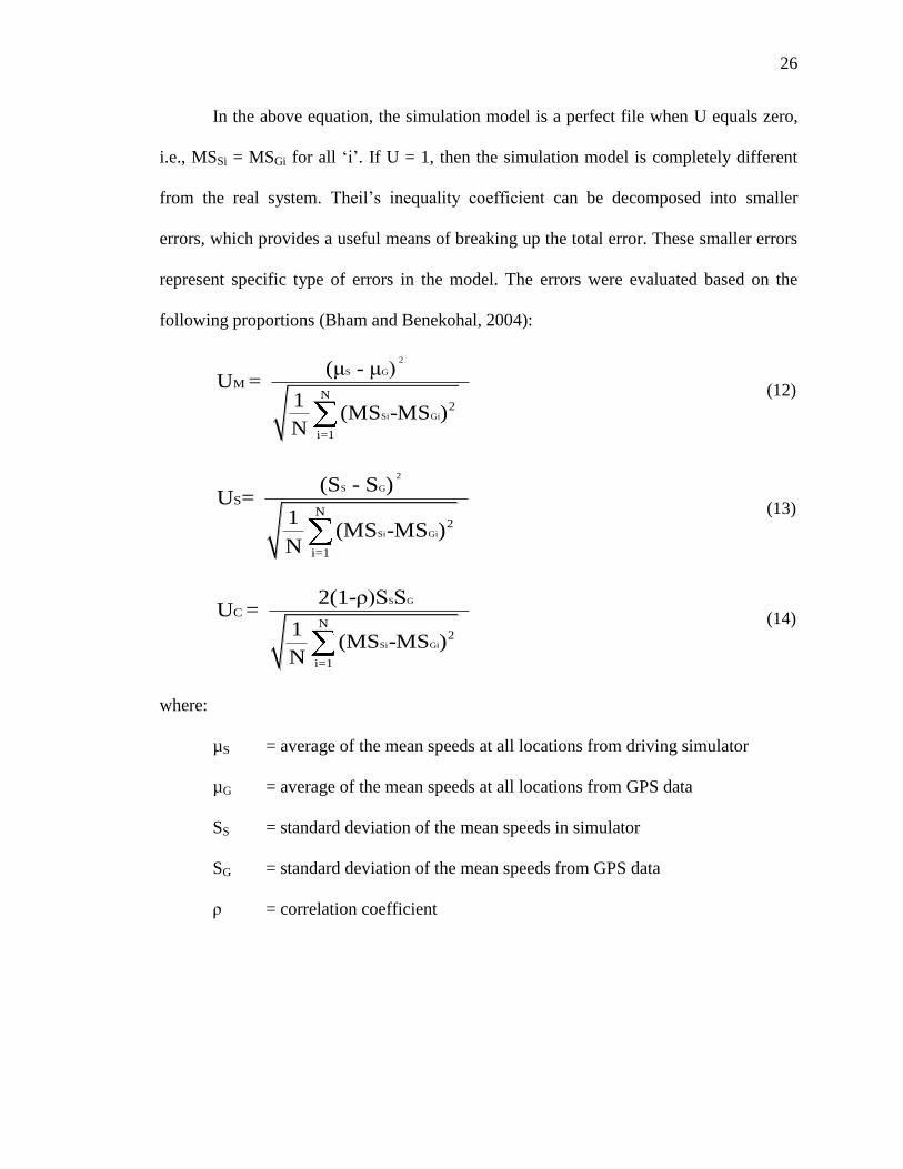
26
In the above equation, the simulation model is a perfect file when U equals zero,
i.e., MSSi = MSGi for all ‗i‘. If U = 1, then the simulation model is completely different
from the real system. Theil‘s inequality coefficient can be decomposed into smaller
errors, which provides a useful means of breaking up the total error. These smaller errors
represent specific type of errors in the model. The errors were evaluated based on the
following proportions (Bham and Benekohal, 2004):
2
S G
Si Gi
M N
2
i=1
(μ - μ ) U =
1(MS -MS )
N
(12)
2
S G
Si Gi
SN
2
i=1
(S - S ) U =
1(MS -MS )
N
(13)
S G
Si Gi
C N
2
i=1
2(1-ρ)S S U =
1(MS -MS )
N
(14)
where:
µS = average of the mean speeds at all locations from driving simulator
µG = average of the mean speeds at all locations from GPS data
SS = standard deviation of the mean speeds in simulator
SG = standard deviation of the mean speeds from GPS data
ρ = correlation coefficient

27
ρ can be calculated as:
Si S Gn G
Si Gi
N
i=1
N N2 2
i=1 i=1
1(MS - μ ) (MS - μ )
Nρ =
1 1(MS ) + (MS )
N N
(15)
The proportions UM, US, and UC are called the bias, the variance and the
covariance proportions of U, respectively. They are useful as a means of breaking down
the differences in the mean speeds from the simulator and the GPS into its characteristic
sources. UM is an indication of systematic error, since it measures the extent to which the
mean values of the simulated and GPS data deviate from each other. A large value of UM
would mean that a systematic bias was present and the mean speeds were different from
the driving simulator and the GPS. A high value of US would mean that the GPS data
varied considerably while the simulator data showed little variation, or vice versa. UC
measures nonsystematic errors, i.e., it represents the remaining errors after deviations
from mean speeds have been accounted. For any value of U > 0, the ideal profiles of
speeds from the driving simulator and the GPS over the three sources of errors are UM =
0, US = 0, and UC = 1 (Pindyck and Rubinfeld, 1998).
For use in the error tests, the speeds observed using the GPS over the roadway
from MM 181.6 to MM 180.0 were compared with those observed from the driving
simulator. This comparison was carried out by calculating the mean speeds for every 500
feet for every run. The driving simulator and the GPS data consisted of speeds captured at
every 0.1 seconds. The mean speeds over each highway section for each run, was
determined as presented below.

28
The mean speed, SXin, at every section ‗i‘ for nth
run with ‗m‘ speed
measurements captured at every 0.1 seconds, presented in Figure 3, was determined as:
Xin
m m-1 2 1
m m-1 2 1
(y -y )+.......(y -y )S =
(t -t )+.......(t -t )
(16)
where:
X = ‗S‘ for driving simulator, ‗G‘ for GPS
ym = distance coordinate at mth
point
tm = time coordinate at mth
point
Figure 3. Calculation of Mean Speed at a Section
Since the time intervals between data points were equal, for simplicity the mean speed
can be rewritten and computed as:
Xin
1 ms +.......+sS =
m (17)
where:
sm = speed obtained at a point from the GPS or driving simulator at the mth
point
The mean speed (MSXi) for ‗n‘ runs over section ‗i‘ was determined as the
arithmetic mean of Sxi.
29
4. OBJECTIVE EVALUATION
The objective evaluation of the driving simulator was performed in terms of both
qualitative and quantitative validations. The qualitative validation compared the driver
behaviors from the driving simulator with those obtained from the field study. The
quantitative validation involved the absolute and the relative validations by statistical
comparison of the mean speeds obtained from the driving simulator with those from the
video data at specific locations along the roadway.
4.1. Qualitative Validation
As quantitative validation is detailed and time consuming, this study introduces
qualitative validation as a first step before more detailed testing is carried out. The
qualitative validation evaluates if the quantitative validation should be carried out or
improvements in the driving simulator are required. Qualitative validation requires
graphical comparison of results from the results of the driving simulator and the real
world. It is, therefore, proposed that GPS data be collected in the real world for
comparison with the driving simulator data. GPS data also provides the capability to
validate along the highway rather than mainly at specific locations. Data collected at
specific locations can supplement the GPS data collected for more detailed validation.
Qualitative validation was carried out to test if the driver behavior in the simulator
was similar to the real world. Figure 4 shows the comparison of speeds obtained from
the video data, the GPS data and the driving simulator. It was observed that the speeds of
the drivers did not depend on the elevation of the section but was influenced by the
advance warning signs, the taper area and the construction area of the work zone.

30
It was found that the driver behavior was similar at specific locations along the
roadway in the real world captured by the video recording and in the driving simulator. In
both cases, the speeds of the drivers decreased from the location at the left lane closed
sign (LLC1) to the location at the end of the work zone (EW). Thus, further evaluation
was carried out to validate the driving simulator quantitatively with the video data.
Additionally, the driver behavior was qualitatively validated along the entire
roadway in the simulator and in the real world by comparing the simulator data and the
GPS data. The comparison of the speed profiles from the GPS study and the driving
simulator study seems to point to the reliability in the results from the simulator. Out of
the 18 sections along the roadway shown in Figure 4, the driver behavior in the simulator
and that from the GPS seems to be similar at 17 sections. The speeds of the drivers
decreased from the RWA to the DNP in both the GPS and the driving simulator data. In
both cases, the mean speeds of the drivers increased from the DNP to the LLC1. As the
drivers approached the LLC2, the mean speed measured by the GPS and driving
simulator decreased. Five hundred feet after the speed limit sign (SL) the driver behavior
in the simulator was different from that in the real world because there was significant
speed reduction in the driving simulator. This reduction in speed can be attributed to the
slowing down of drivers to reduce their speed after noticing the reduced speed limit sign.
Additionally, the lack of motion base in driving simulator lowers the perception of the
speed to which the drivers were trying to reduce. The drivers increased their speed from
LLC2 till they noticed the construction zone (1000 feet before the CA) and then
decreased as they approached the CA. Thus, good correspondence was noted between the
driver behavior in the simulator data and the field data (GPS) which indicated the relative

31
validity of the driving simulator. Thus, further evaluation was carried out to statistically
test the absolute and relative validities of the driving simulator.
Figure 4. Comparison of speeds from Video Recording, GPS, and Driving Simulator
4.2. Quantitative Validation
The qualitative validation indicated a good correspondence in the driver behavior
in the real world and in the driving simulator at specific locations and also along the
entire roadway. Thus, quantitative validation was carried out to evaluate the absolute and
relative validities of the driving simulator.
4.2.1. At Specific Locations. The mean speeds from the video recording were
compared with those from the driving simulator at the following locations: i) upstream of
the work zone (FW), ii) left lane closed sign (LLC1), iii) ‗60 mph‘ speed limit sign (SL),
iv) inside the construction zone (CA), and the end of the work zone (EW). Table 2 shows
the means and the standard deviations of speeds from the video data (MSR) and those

32
from the simulator (MSS) at the five locations. The comparison of the mean speeds from
the field data with those from the simulator demonstrates the relative validity of the
simulation. The difference between the mean speeds (MSS – MSR) ranged from -1.5 mph
(at the speed limit sign SL) to 1.8 mph (at the freeway location FW). For the locations SL
and the CA, the mean speeds were 1.5 mph and 0.9 mph lower for the simulator
compared to the field study.
Table 2. Results of Field Study and Driving Simulator Study
Locations
Video Data Driving Simulator Data
MSS – MSR
D
Number
of
Vehicles
(nR)
Mean
Speed
(MSR)
Standard
Deviation
(SR )
Shapiro-
Wilk
Mean
Speed
(MSS)
Standard
Deviation
(SS )
Shapiro
-Wilk
(mph) (p-value) (mph) (p-
value) (mph)
(%)
FW 41 68.5 8.9 0.18 70.3 5.4 0.18 1.8 2.6
LLC1 66 63.2 9.1 0.39 63.8 7.0 0.62 0.6 0.9
SL 59 62.5 4.9 0.13 61.0 5.0 0.18 -1.5 -2.4
CA 16 61.5 2.7 0.17 60.6 5.6 0.16 -0.9 -1.5
EW 85 59.3 8.4 0.13 60.5 3.3 0.78 1.2 2.0
Number of participants in the driving simulator study (nS) = 46
On the freeway upstream of the work zone (FW), the percentage deviation
equaled 2.6% which indicated that the drivers drove at higher speeds in the simulator.
This value shows that the speeds recorded in the simulator were higher for the less
demanding location, perhaps due to lower risk of crashes in the simulator than in the real
world. This finding was consistent with those of the study conducted to validate the use
33
of a driving simulator for a two-lane rural road (Bella, 2008). At the location of the speed
limit sign, the deviation was -2.4%, indicating that the speeds recorded in the simulator
were lower for the locations where the drivers had to make relatively complex
maneuvers. This finding was consistent with the validation of a driving simulator for a
crossover work zone (Bella, 2005). Bella also found that the speeds were lower in the
simulator than in the real world at the speed limit sign in the advance warning area. Thus,
the speeds were higher in the simulator when the drivers accelerate on the freeway
whereas they were lower when the drivers decelerate in the work zone.
From Table 2, the standard deviation was found to be higher in the real world than
in the driving simulator at FW, EW, and the LLC1 locations. This indicated larger
variations in the speeds of drivers in the real world compared to the driving simulator
when they were not reducing their speeds. It must be kept in mind that driving in the
simulator is not affected by other vehicles. The standard deviation at the location CA was
higher in the driving simulator compared to the real world. This indicated lowest
variation in speeds from the field data as very limited data were available from this
location because of congested traffic flow, i.e. most vehicles were not free flowing.
A Shapiro-Wilk test was carried out on the video data and the driving simulator
data collected at five locations and the results are presented in Table 2. The test revealed
that the data were approximately normally distributed, i.e., the p-values were greater than
0.05 and it fitted a Gaussian distribution at the five locations in the field and also in the
driving simulator. Figure 5 shows the distribution of speeds at LLC1.
Table 3 shows the results of F-test, t-test and power analysis for each location.
The results of F-test indicate that the null hypothesis was accepted, that is, the variance of

34
the speeds in the driving simulator and in the field was equal at the SL location. Since the
variance was unequal at four locations as evidenced from Table 3, the field observations
and the simulator results were compared at each location using tests that does not assume
equality of variance. The t-test indicated that the difference in the mean speeds lies within
the confidence interval. Thus, the null hypothesis was accepted at a 5% level of
significance at the five locations, and there was no significant difference between the
mean speeds in the driving simulator and those in the real world. Therefore, the absolute
validity of the driving simulator was obtained. Also, the relative validity of the driving
simulator was obtained since the speeds were not statistically different and varied in the
same direction in the video data and in the driving simulator data.
Figure 5. Distribution of Speeds Observed from the Video data and from the
Driving Simulator Data at LLC1

35
The power of the t-test ranged from 68% upstream of the work zone (FW) to 93%
at the location of the speed limit sign (SL). These values indicate a very low probability
that a false null hypothesis will be accepted by mistake. In other words, the power
analysis indicated a low probability of type II error in the work zone advance warning
area and in the construction activity area. The possibility of such errors was higher at the
freeway location.
Table 3. F-Test, t-Test and Power Analysis: Field data versus Driving Simulator
data
Locations
F-test t-test
F-ratio F-
critical
Result
(H0) tC DF* CI^
Power
(1- β)
Result
(H0)
FW 2.71 1.65 Rejected 1.67 64 ±2.68 0.68 Accepted
LLC1 1.69 1.59 Rejected 1.66 109 ±2.55 0.93 Accepted
SL 1.04 1.69 Accepted 1.66 103 ±1.64 0.93 Accepted
CA 4.13 2.13 Rejected 1.67 53 ±0.97 0.89 Accepted
EW 6.48 1.56 Rejected 1.65 120 ±1.69 0.89 Accepted
*DF = Degrees of freedom for the t-test
^CI = Confidence Interval
Thus, the results of the statistical analysis indicate that the driving simulator
experiments were valid, both relatively and absolutely, at all the locations and confirm
that the driving simulator yields speeds similar to those observed in the real world and the
differences in the mean speeds were insignificant. The lower speeds in the simulator at
the location of a complex maneuver may reflect the lack of motion cues that influence
driver behavior in the real world.

36
4.2.2. Along the Roadway. Since qualitative validation indicated similar driver
behavior in both the driving simulator and the field captured by the GPS, the quantitative
validation was carried out using error tests to evaluate the absolute and relative validity of
the driving simulator along the simulated roadway. As stated in the previous section, the
error tests were conducted for the mean speeds calculated at every 500 feet from the
driving simulator and the GPS. The Theil inequality coefficient (U = 0.022) indicated that
the driving simulator was perfect in predicting the driver behavior in real world.
As described previously, the Theil inequality coefficient was further decomposed
into three proportions: bias, variance, and covariance. The bias proportion (UM = 0)
indicated that the mean speed from the simulator was the same as the real world i.e., there
was no systematic errors. This indicated the absolute validity of the simulator along the
entire roadway. This was also indicated by the t-tests conducted at specific locations. The
variance proportion (US = 0.13) was not significant or troubling but the dispersion in the
speeds were experienced in the real world and in the driving simulator. The small sample
of the GPS data might be one of the reasons for the small difference in the degree of
variability. The covariance proportion (UC = 0.87) was high, demonstrating that the
speeds in the driving simulator significantly co-varied with the real world. Thus, the
relative validity of the driving simulator was obtained along the roadway. The small
nonsystematic error indicated by the covariance proportion is less worrisome and can be
reduced by decreasing the variance proportion.
Thus from the error tests, the absolute and relative validity of the driving
simulator was also obtained by comparing the speeds from the driving simulator along
the entire roadway with those obtained by the GPS from the real world. With the larger
37
sample size from the GPS and improvements to the driving simulator, the variance
proportion and covariance proportions are expected to approach 0 and 1, respectively.
5. SUBJECTIVE EVALUATION
A post-experiment survey of participants evaluated the driving simulator based on
their driving experience. The participants completed a questionnaire that surveyed them
to rate the realism of various driving simulator components and the various aspects of the
simulated driving scenario. The components included the brake pedal, steering wheel,
and gas pedal whereas the aspects of the driving scenario included the surrounding terrain
along the road, the simulated road geometry constructed using the GPS data, and the
drivers‘ feeling of the simulated vehicle. For each criterion, participants rated the driving
simulator on a scale of 1 to 7, with 1 indicating unrealistic and 7 very realistic. The mean
ratings for each criterion were calculated by determining the arithmetic mean. Table 4
shows these ratings calculated for each criterion.
Table 4. Results of Subjective Evaluation
Simulator Components Driving Scenario
Brake Pedal Steering
Wheel Gas Pedal
Surrounding
Terrain Road Geometry
Feel of
driving
Mean
Rating 5.0 5.8 5.3 5.5 5.9 5.2
The results show that the participants were comfortable with the driving simulator
as they rated the various components and characteristics to be realistic. All of the values

38
were much higher than the neutral value of 4. The steering wheel was rated highest
among the driving simulator components. Among the various aspects of the driving
scenario, road geometry was rated highest indicating that the use of GPS to construct the
road scenario effectively replicates the real world.
6. CONCLUSIONS AND RECOMMENDATIONS
This paper presents the framework for objective and subjective evaluations of a
driving simulator. Validation was divided into quantitative and qualitative validations,
which were performed along the roadway and at specific locations where additional data
were collected. The validation of the driving simulator was performed by comparing the
vehicle speeds from a real work zone with those from the simulator.
The qualitative comparison indicated that the driver behavior was similar in the
driving simulator and in the real world at specific locations and also along the entire
roadway. Since the qualitative validation indicated good correspondence in the driver
behavior, the quantitative validation was performed. The quantitative validation was
carried out using statistical tests to evaluate absolute and relative validity at specific
locations. For the quantitative validation at specific locations, the absolute and relative
validity of the driving simulator were analyzed at five locations and t-tests were
conducted. From these tests it was concluded that the field speeds and the driving
simulator speeds were essentially the same. Therefore, the driving simulator was
validated absolutely and relatively at these locations.
From the error tests, the bias proportion showed that the mean speed of the GPS
data and that of the simulator data were the same. This indicated the absolute validity of
the driving simulator along the entire roadway. The high value of covariance proportion

39
also demonstrated the relative validity of the driving simulator. The subjective evaluation
of the driving simulator showed that the participants rated the driving simulator realistic
in both the simulator components (for braking, acceleration, and steering) and the driving
scenarios (surrounding terrain, road geometry, and feel of driving). Road geometry was
rated most realistic, indicating that the use of GPS to reconstruct the road in a simulator
was effective and provided realistic experience.
ACKNOWLEDGEMENTS
The authors gratefully acknowledge research support for this project from the
Intelligent Systems Center at the Missouri University of Science and Technology, Rolla,
Missouri.
REFERENCES
Arnedt, J. T., Owens, J., Crouch, M., Stahl, J., and Carskadon, M. A. (2005).
Neurobehavioral Performance of Residents After Heavy Night Call versus After Alcohol
Ingestion. The Journal of the American Medical Association, Vol. 294, pp. 1025-1033.
Bella, F. (2005). Validation of a Driving Simulator for Work Zone Design.
Transportation Research Record, 1937, Washington, D.C., pp. 136–144.
Bella, F. (2005a). Operating speed predicting models on two-lane rural roads from
driving simulation. In: Proceedings of the 84th
Annual Meeting of the Transportation
Research Board, Washington, D.C.

40
Bella, F. (2008). Driving simulator for speed research on two-lane rural roads. Accident
Analysis and Prevention, Vol. 40, No. 3, pp. 1078-87.
Bham, G. H., Leu, M. C., Mathur, D. R., and Javvadi, B. S. (2009). Evaluation of Vehicle
Mounted Attenuator (VMA) Markings Using a Driving Simulator for Mobile Work
Zones. In: Proceedings of the 88th
Annual Meeting of the Transportation Research Board,
Washington, D.C.
Bham, G. H. and Benekohal, R. F. (2004), A High Fidelity Traffic Simulation Model
based on Cellular Automata and Car-Following Concepts. Transportation Research Part
C: Emerging Technologies, Vol. 12, No. 1, pp. 1-32.
Bittner Jr., A. C., Simsek, O., Levison, W. H., and Campbell, J. L. (2002). On-road
versus simulator data in driver model development driver performance model experience.
Transportation Research Record, 1803, Washington, D.C., pp. 38–44.
Blaauw, G. J. (1982). Driving experience and task demands in simulator and
instrumented car a validation study. Human Factors, Vol. 24, pp. 473–486.
Blana, E. (1997). The Pros and Cons of Validating Simulators Regarding Driving
Behavior. In Driving Simulation Conference 97, Lyon, France, pp. 125–135.

41
Cohran, W.G., and Cox, G.M. (1957). Experimental Designs, 2nd
Edition, John Wiley and
Sons Inc, New York.
Fairclough, S. H., and Graham, R. (1999). Impairment of Driving Performance Caused
by Sleep Deprivation or Alcohol: A Comparative Study. Human Factors: The Journal of
the Human Factors and Ergonomics Society, Vol. 41, No. 1, pp. 118-128.
Godley, S., Triggs, J., and Fildes, B. (2002). Driving simulator validation for speed
research. Accident Analysis and Prevention, Vol. 34, No. 12, pp. 589–600.
Kaptein, N., Theeuwes, J., and Van Der Horst, R. (1996). Driving simulator validity:
Some considerations. Transportation Research Record, 1550, pp. 30–36.
Klee, H., Bauer, C., and Al-Deek, H. (1999). Preliminary validation of a driving
simulator based on forward speed. Transportation Research Record, 1689, pp. 33–39.
Laser Technology Inc. (2010),
<http://www.lasertech.com/content/pdfs/ULCompact_Spec.pdf> (Mar. 7th
, 2010)
Likert, R. (1932). A Technique for the Measurement of Attitudes. Archives of
Psychology 140, 55.

42
McAvoy, D., Schattler, K., and Datta, T. (2007). Driving simulator validation for
nighttime construction work zone devices. 86th
Annual Meeting of the Transportation
Research Board, Washington, D.C.
Pindyck, R.S. and Rubinfeld, D.L. (1998). Econometric Models and Economic Forecasts.
fourth ed. McGraw-Hill, NY.
Satterthwaite, F. E. (1946). An Approximate Distribution of Estimates of Variance
Components. Biometrics, Bulletin 2, pp. 110–114.
Shapiro, S. S. and Wilk, M. B. (1965). An analysis of variance test for normality
(complete samples). Biometrika, 52, No. 3/4, pp. 591-611.
Smith, S.A. (1985). Freeway Data Collection for Studying Vehicle Interactions.
Technical Report FHWA/RD-85/108, Federal Highway Administration, Office of
Research, Washington D.C. Trimble (2010), <http://www.trimble.com> (Mar. 7th
, 2010)
Tornos, J. (1998). Driving behaviour in a real and a simulated road tunnel—a validation
Study. Accident Analysis and Prevention, Vol. 30, No. 4, pp. 497–503.
Wang, Y., Zhang E., Zhang W., Leu M. C., and Zeng, H. (2006). Development of A
Low-cost Driving Simulation System for Safety Study and Training. Proceedings of the
Driving Simulation Conference-Asia/Pacific, Tsukuba, Japan, May 31-Jun. 2.

43
Yan, X., Abdel-Aty, M., Radwan, E., Wang, X., and Chilakapati, P. (2008). Validating a
Driving Simulator using Surrogate Safety Measures. Accident Analysis and Prevention,
Vol. 40, 274–288.

44
2. YOUNG DRIVER’S EVALUATION OF VEHICLE MOUNTED
ATTENUATOR MARKINGS IN WORK ZONES USING A DRIVING
SIMULATOR
Ghulam H. Bham1, Durga Raj Mathur
2, Ming C. Leu
2, Manoj Vallati
2
Civil, Architecture and Environmental Engineering1
Mechanical and Aerospace Engineering2
Missouri University of Science and Technology (Missouri S&T)
ABSTRACT
This paper evaluates the effectiveness of four vehicle mounted attenuator (VMA)
striping patterns and color combinations used by the Departments of Transportation
(DOTs) in work zones. A driving simulator was used to evaluate the perception of
seventy-three young participants who drove through virtual highway work zones. Lane
change distance (LCD) was used to analyze their reaction to the VMA markings during
the daytime. An analysis of variance (ANOVA) test was performed to determine the
significant variables affecting the LCD. A pairwise least-square means test was
performed to determine the difference between the LCDs of the markings. A subjective
evaluation was also carried out in which the participants ranked the markings based on
different criteria. The participants were also surveyed on the features of the individual
markings and their most preferred pattern. The results of the objective and subjective
evaluation were consistent, and they suggested that overall the red and white
checkerboard pattern was the most effective and preferred among the four markings. A
DOT survey conducted in conjunction with this study indicated that the yellow and black

45
inverted ‗V‘ pattern was widely used in the United States as it was provided by most
VMA suppliers.
Key words: vehicle mounted attenuator (VMA), driving simulator, work zone, driver
behavior, traffic control devices (TCD)
1. INTRODUCTION
Work zone safety is a high priority for transportation agencies and the highway
construction industry because of increasing work zone fatalities. The number of such
fatalities grew in the United States by nearly 45% between 1997 and 2006, from 693 to
1004 (NWZSIC, 2010). Additionally, younger drivers between the ages of 18 and 35
were involved in 56% of all fatal crashes for 2008. Similarly, younger drivers were
involved in 58% of all fatal work zone crashes (FARS, 2010). Missouri reported 163
fatalities between 2005 and 2007 for all ages (Crash Data, 2007) in work zones. It is
imperative that highway safety be improved with an objective of reducing the number of
fatalities and severe injuries. Safety improvements can generally adopt one of two
approaches. The first approach focuses on protecting vehicle occupants in the event of a
crash. The second approach focuses on preventing crashes. This present paper addresses
the second approach.
Crash cushions mounted on the rear of vehicles are called vehicle mounted
attenuators (VMAs). They have been used successfully for many years to reduce the
severity of rear-end collisions in work zones. The Manual on Uniform Traffic Control
Devices (2003) and the American Association of State Highway and Transportation

46
Officials (AASHTO) Roadside Design Guide (2002) both contain general guidelines for
VMAs. However, neither publication includes recommendations for striping patterns
and/or colors for these devices. The predominant color combinations used by the United
States Departments of Transportation (DOTs) are yellow and black, orange and white,
red and white, and lime green and black in an inverted ‗V‘, striped or checkerboard
design, but other options have also been used. Some states have experimented with a
vertical striping or checkerboard patterns in red and white. Figure 1 shows four striping
patterns and color combinations used by DOTs in the United States.
(a) Lime Green and Black Inverted ‗V‘ Pattern (b) Red and White Checkerboard Pattern
(c)Yellow and Black Inverted ‗V‘ Pattern (d) Orange and White Vertical Stripes Pattern
FIGURE 1. Vehicle Mounted Attenuator Markings
This study evaluated the driver perception of the effectiveness of four striping
patterns and color combinations for VMAs, as shown in Figure 1, using both objective
evaluation and a subjective survey. Of particular concern was the use of an inverted ‗V‘
design when the following vehicles do not have the option of passing on either side of the

47
work vehicle. The importance of contrast with the VMA truck color was also an issue of
interest. The results of this study can help state DOTs to select the most effective color
and striping patterns for VMAs, thereby improving safety and operations in work zones
on high-speed, high-volume roadways. As part of this study, a survey questionnaire of
state DOTs evaluated their use and policies regarding VMAs. The results of this survey
are also presented in the paper.
Driver perception and behavior can be evaluated by field studies or using a
driving simulator. Field data collection is expensive and can test only a limited number of
TCDs. Driving simulator studies, however, permit the study of hazardous driving
situations that cannot be safely replicated during field tests. Such studies are also efficient
and inexpensive, facilitating the collection of a wide range of data. They are repeatable,
and they permit easy and safe replication of numerous scenarios to evaluate subjects‘
reaction to multiple TCDs.
2. LITERATURE REVIEW
Construction and maintenance work on streets and highways is dangerous,
especially on high-speed highways. The safety of construction operations has received
much attention over the past several years. Efforts to improve safety have increased
substantially, particularly in the wake of a fatal accident in Washington D.C. in 1975
(Mackay and John, 1995). However, roadway fatalities have reduced but crash frequency
has continued to increase, probably due to an increase in highway construction activities.
Preventing crashes and reducing the severity of crashes require anticipation of driver
reactions to specific situations.

48
Research by Humphrey and Sullivan (1991) on the effectiveness of VMAs
indicated that these devices save about $23,000 per crash and reduce damage to the
maintenance vehicle. The study indicated that injury rates were higher for maintenance
vehicles not equipped with VMAs. Additionally, it demonstrated that the cost of crashes
is considerably higher when no VMAs were used.
A field study carried out on VMA best practices in New Zealand (Smith,
Edwards, O‘Neil, and Goluchowski, 2006) reported that positioning an advance warning
system 1312 feet from a VMA during daytime conditions performed better than other
practices, resulting in 27.7% fewer drivers reacting in the last 984 feet and at least 25.4%
fewer drivers reacting in the last 700 feet. The setup of VMA with the advance warning
system fitted with strobe lights, and a message board with words stating ‗Left Lane
Closed‘ achieved mean recognition distance of 1494 feet during the daytime conditions.
Another study (Steele and Vavrik, 2009) around lane closures with an aim to improve the
safety of moving lane closures found that 94.4% of drivers moved out of the closed lane
at least 500 feet before the start of the taper at a rural test site compared to 86.8% for an
urban area.
Many studies on work zones have compared the use of different colors. Kamyab
and Storm (2001) used a fluorescent yellow-green background with an orange sign and
found that this improved the contrast between the sign and the orange DOT truck. They
conducted a driver survey on the visibility of the sign with and without the fluorescent
background. The report presented the differences in terms of traffic volume with and
without the fluorescence background. Another study by Atchley (2006), however,
suggested that fluorescent traffic signs had no advantage over non-fluorescent signs.

49
The literature reviewed offered no specific guidelines for selecting color or
striping patterns for use with VMAs. The present research is a first major step toward
determining the best VMA patterns for use in construction zones.
3. METHODOLOGY
Participants were tested in a driving simulator to evaluate their perception and
behavior objectively, and were surveyed subjectively. A survey of state DOTs evaluated
their use and policy regarding VMAs. This section describes the details of DOT survey,
the driving simulator experimental setup, the statistical data analysis conducted to
evaluate the driver behavior, and the details of the questionnaires used.
3.1. DOT Survey
Fifty state DOTs were contacted and requested to complete the VMA survey on-
line. The survey was carried out for six weeks between February and March of 2008 and
30 states responded. The survey comprised of five parts: 1) General information related
to VMAs, 2) Policy pertaining to VMA usage, 3) VMA striping patterns and colors in
use, 4) VMA evaluation and effectiveness, and 5) VMA crash data. The results of the
web survey are summarized in the next section.
3.2. Driving Simulator Study
3.2.1. Missouri S & T Driving Simulator
A fixed-base driving simulator for this study uses a Ford Ranger pick-up truck,
three LCD projectors, a projection screen, and three networked computers. The computer

50
that processes the motion of the vehicle is defined as the master; the other two computers
are defined as slaves. The vehicle is equipped with a speedometer and other standard
components. Different types of sensors are used to measure the steering operation,
vehicle position and speed, acceleration/deceleration, and braking. The screen has an arc
angle of 54.6°, an arc width of 25 feet and a height of 6.6 feet. The field of view is around
120°.
The resolution of the visual scene generated by the master is 1024×768 pixels,
and that for the slaves is 800×1200 pixels; the refresh rate is 30 to 60 Hertz depending on
the scene complexity. The system is also equipped with a system that replicates the sound
of an engine. Wang et al. (2006) provided a more detailed description of the system
structure, projection system, and the data acquisition process.
3.2.2. Work Zone Setup and Configuration
A virtual work zone scenario was developed to resemble a 4-lane rural divided
highway with a median and four consecutive work zones. The highway was
approximately eight miles long with the first work zone setup at 1.5 miles and each work
zone was 0.5 miles long and 1.5 miles apart. Figure 2 shows the setup of traffic control
devices, two VMAs and a construction vehicle on the closed lane. The colors and patterns
of the four VMAs changed randomly for the participants for the four work zones. The
two VMAs within a single work zone were kept identical.
A virtual work zone environment was created for the simulation according to
MUTCD (2003) specifications for a partial lane closure on a divided highway. These
guidelines specify sign spacings, taper lengths, and optional buffer length channelizer

51
spacings for various speed limits, sign heights, and work zone lengths. Various signs
were set up to replicate a construction zone on a freeway. The first 1.5 miles of the
freeway had a speed limit of 70 mph, indicated by a regulatory speed limit sign at the
beginning of the section. Traffic signs were placed along the right side of the roadway
500 feet apart, as shown in Figure 2, starting with ‗Road Work Ahead‘ warning sign
located 1.5 miles before the beginning of the work zone. The four remaining signs were
placed in the following order: ‗Speed Limit 45 mph‘, ‗Right Lane Closed Ahead,‘ ‗Speed
Limit 45 mph,‘ and ‗Right Lane Closed Ahead‘. The construction zone was 1300 feet
long with barriers on the lane marking. The construction zone consisted of a shadow
vehicle with a VMA, a work vehicle with a VMA, and a construction vehicle. These
vehicles were separated by a distance of 550 feet from the center of the vehicle.
FIGURE 2. Work Zone Configuration

52
3.2.3. Participants
Prior to scheduling the experiment, the subjects were screened using a
questionnaire to inquire if they had a US driver‘s license, no health problems that would
affect driving, and they do not suffer from motion sickness. Seventy-three drivers met the
requirements and participated in the experiment. Participants were mostly students, some
staff and faculty from Missouri S&T and residents of Rolla, Missouri. The drivers were
between the ages of 18 and 35 years with an average age of 22.2 years and a standard
deviation of 2.34 years. Twenty three participants were female and 50 were male. Of the
73 participants, one had been driving for more than 15 years, 49 had been driving
between 5 and 15 years, and 23 had been driving between 1 and 5 years. All participants
had previously encountered VMAs in highway work zones.
3.2.4. Pre- and Post-Experiment Questionnaires
The participants were surveyed before the start and after the end of the driving
simulator experiment. The pre-experiment questionnaire inquired about health issues
specifically that could affect their driving in a simulator, and consumption of
alcohol/drug use during the last 24 hours. This was carried out to ensure that drivers were
alert and eligible for participation in the experiment on the day of the experiment. All
participants had normal or corrected-to-normal vision and no one reported color
deficiency. The participants were also checked for validity of the US driving license and
anyone found with an invalid license was turned away from the experiment.
After the driving simulator experiment, each participant was asked to complete a
post-experiment questionnaire. This questionnaire served as the subjective evaluation of

53
the VMA patterns based on the participant‘s experience with the driving simulator. The
participants were asked to rank (1 highest and 4 lowest) the four patterns based on the
following criteria: i) visibility, ii) alerting drivers to work zone, iii) capturing driver‘s
attention, and iv) color contrast with the VMA vehicle. Visibility was used as a criterion
for evaluation of the VMAs because it is important with regard to specific environmental
conditions such as weather and times of the day. A pattern that is easily visible from a
distance would alert the driver to construction activity downstream, thus reducing the risk
of a crash. The pattern that captures the most attention of the drivers would cause drivers
to notice a work zone and change lanes before approaching the VMA.
Alerting drivers to work zones and contrasting the VMA pattern with the VMA
vehicle were also used as criteria. The participants were also asked to rank features of
individual patterns. This was carried out for participants to indicate their preferences for
each pattern based on pattern design, color combination, and color contrast using a scale
of 1 to 3, with 1 indicating most liked and 3 indicating least liked. The participants were
also asked which pattern they preferred and how they interpreted the meaning of features
of the patterns.
3.2.5. Experiment
The participants were first given a brief introduction to the driving simulator and
advised to adhere to traffic laws and drive as they would in normal traffic conditions. To
familiarize the participants with the driving simulator, the environment, and the
instructions, participants first drove through a trial scenario similar to that used in the
experiment. Typically, each participant first drove for several minutes during the trial run

54
and then drove through the experimental scenario with the four construction zones. The
VMA patterns appeared in random order. Driver behavior data was collected by various
sensors for every 0.1 seconds.
3.2.6. Data Analysis
The drivers‘ acceleration/deceleration, speed, position and steering angle were the
main variables measured during the driving simulator experiment for use with the
objective evaluation. From vehicle positions, the distances from the point of lane change
on the closed lane to the VMA were obtained. This distance, called the lane change
distance (LCD), was used as the criterion for determining the effectiveness of a VMA
pattern. LCD was measured from the point where the driver began to steer continuously
out of the right lane (closed lane) and towards the left lane, achieving the maximum
steering angle. The drivers were assumed to respond to the appearance of the VMA
pattern. This measure was selected because most DOTs that responded to the survey had
used it along with crash data to determine the effectiveness of VMAs in work zones.
Further, Bham et al. (2009) found that the speed reduction identification distance, i.e. the
distance from the VMA at which the driver starts decelerating, should not be used to
evaluate VMA patterns because drivers reduce their speed in response to advance
warning signs.
The experiment was conducted such that each participant was exposed to the
different VMA markings in a single run, with the markings in random order. Therefore,
the appropriate statistical design for this experiment was a split-plot, with each
participant represented as a main-plot and the four work zones as a sub-plot. Gender was

55
used as the main-plot factor (independent variable) and the pattern was used as the sub-
plot factor. The analysis of variance (ANOVA) was carried out to test the statistical
significance of gender and VMA patterns on the mean LCD. The test was conducted
using the Statistical Analysis System (SAS, 2008) software package. The statistical
significance of the independent variables (factors) was determined at the 0.05
significance.
The ANOVA results showed a significant difference among the LCDs, therefore,
pairwise comparisons of least-square means (LSM) between patterns were performed in
SAS using the LSMEANS command. LSM are predicted values, based on the model
fitted across the values of a categorical effect where other model factors are held constant
by setting them to the least-square estimate of their means. If the experiment is a
balanced one, where each combination of factors (i.e., independent variables) were
replicated an equal number of times, least-square means will be the same as regular
sample means. In this experiment, however, we did not have equal samples within factor
combinations and therefore the use of least-square means is warranted.
The LSM test was conducted by employing the Tukey-Kramer adjustment, which
uses the approximation described by Kramer (1956). It was used to accommodate the
unbalanced data and provide good control of the Type 1 error rate. To further analyze the
data, a Kolmogorov-Smirnov (KS) test was also conducted using SAS to ascertain if
there is a statistically significant difference between the lane change frequency
distributions. The KS procedure tests the null hypothesis of any significant difference
between the LCD cumulative distributions for the four VMA patterns by looking at the
difference at the point of maximum separation between the distributions. This is in

56
contrast to the ANOVA based test described earlier, which looked at the differences
between the means. A significant difference between the cumulative frequency
distributions for two patterns would imply that the lane change behavior of drivers was
different between the patterns. Straightforward use of the KS test on the distribution of
participant‘s LCD would reduce the power of the test because of the heterogeneity of
driving styles as that would add to the ―noise‖ in the data. The effect of an individual
participant‘s driving style was eliminated by calculating the dependent variable as the
difference between the pattern LCD for a participant and the average LCD of that
participant for the four patterns. This distance was used instead of the actual LCD of the
patterns for the KS test. The KS test was conducted at 0.05 level of significance.
To supplement the objective evaluation, all participants completed a post-
experiment questionnaire for subjective evaluation of the VMA markings. The subjective
evaluation served as an opinion poll of the participants regarding the four patterns in
contrast to measuring the effect of the patterns on their actual driving behavior. The
results of the subjective evaluation should be carefully interpreted as they present the
perception of the drivers. Participants ranked the four VMAs based on each criterion, as
described above, on a scale of 1 to 4, with 1 indicating excellent, 2 good, 3 average, and 4
poor. The mean rank of a pattern for a criterion was calculated by summing up the ranks
given to a pattern and dividing the sum by the total number of participants, thereby
calculating the arithmetic mean. The mean of the ranks for each pattern was compared
against each other.
A statistical test was also carried out to find the significance of pattern preference
by the participants. It should be noted here that the participants ranked the four patterns

57
according to a criterion. Thus, the data for an individual participant provided information
on their first, second, third and the last choice. Further, the ranks for each pattern were
correlated within each individual. The statistical model that was used to analyze this data
can be explained as follows. First, a participant selected his/her first choice (rank = 1, the
highest). Then, among the rest, the next best choice was selected (rank = 2) and so on.
The resulting model is sometimes referred to as the exploded logit model, a discussion of
which can be found in Allison and Christakis (1994). The likelihood function obtained
for this model is exactly the same as the likelihood one would obtain for the stratified
Cox regression analysis and thus can be estimated using the PHREG procedure in SAS
(2008). In this, context, the PHREG procedure estimates the parameters of the model and
provides risk ratios of proportions, which are the odds of a pattern to be ranked 1 (best)
under a particular criterion when compared against a base pattern. For analysis of results,
the yellow and black inverted V pattern was used as the base pattern and the risk ratios
for the rest of the patterns with respect to it were estimated.
4. ANALYSIS AND DISCUSSION OF RESULTS
4.1. DOT Survey Results
This section summarizes the responses from 30 state DOTs. The results of the survey are
presented in different categories below.
4.1.1. VMA Policy
The DOTs were inquired about the policy of VMA usage in work zones. Twenty-
two states (76%) reported the use of VMAs in work zones because it is a transportation

58
agency policy; one state, Delaware, reported its use because of state law; five states
(17%), Rhode Island, Minnesota, Wisconsin, Hawaii, and Massachusetts, use VMAs in
work zones independent of transportation agency policy or state law. All DOTs, except
Minnesota, reported the use of VMAs in work zones. Two states did not respond to this
question.
4.1.2. VMA Striping Patterns and Colors
The DOTs were asked about the different color combinations used with the
VMAs. The survey result is shown in Figure 3(a). Twenty five states indicated the use of
yellow and black for VMAs. Washington D.C. uses all four VMA markings. California
uses three color combinations; yellow-black, orange-white, and red-white. Kansas uses
yellow-black and orange-white, and Texas uses yellow-black and red-white color
combinations. New York does not use any of the four patterns presented in Figure 1; it
uses a yellow-blue color combination. Figure 3(a) graphically presents the DOT‘s use of
different VMA patterns.
The DOTs were also inquired about the type of VMA patterns in use. Twenty-
seven agencies indicated they use inverted ‗V‘ pattern for VMA stripes. California
indicated use of a stripe pattern from the lower left corner to the upper right corner. When
DOTs were asked about the basis for the selection of VMA colors and patterns, out of the
27 state agencies, eight use the VMA patterns and colors provided by VMA suppliers and
11 use these colors and patterns to conform to MUTCD guidelines for work zones,
warning colors, and object markers. Kansas uses an inverted ‗V‘ pattern similar to a Type
III barricade. Delaware and Oregon use yellow and black to make the device stand out

59
from orange and white construction equipment. New York uses yellow and blue to match
the colors of their trucks. Texas and New York use an inverted ‗V‘ pattern to indicate that
vehicles can pass on either side of the truck.
4.1.3. VMA Evaluation and Effectiveness
The agencies were asked if they had tested the patterns and colors used with the
VMAs. Only Texas indicated that they had evaluated various colors and striping patterns
for VMAs. They found that red and white inverted ‗V‘ pattern was most appropriate for
their fleet. Also, the DOTs were asked about the conditions during which the VMAs were
used. Six agencies use VMAs in both daytime and nighttime conditions, whereas three
agencies use them only during the day. Only two agencies, West Virginia and California,
use VMAs during day and nighttimes, and misty/foggy conditions.
The DOTs were also asked if they had evaluated the effectiveness of VMAs in
work zones. Washington, Wisconsin, and Hawaii indicated they had used crash data and
LCD to determine the effectiveness of using VMAs in work zones. Nine agencies only
used crash data as a measure of effectiveness. Rhode Island, Texas, Indiana, and
Washington had used the following measures of effectiveness:
visibility of VMAs (determined through surveys or the use of videos during which
changes in driver behavior were observed),
work zone operation and proximity to traffic,
workers survival rate after car or truck impacts, and visual assessment under various
light conditions.

60
(a) Use of different color combinations by DOTs
Between 20
and 40, 3, 10%
Between 40
and 60, 3, 10%
Between 60
and 100, 0, 0%
More than 100,
1, 3%
N/A, 6, 20%
Less than 20,
17, 57%
(b) Vehicle crashes with VMAs over the last three years based on 30 responses (crash frequency,
number of DOT responses, percentage of DOT responses)
N/A, 7, 23%
Marginal change
(within 10%), 7,
23%
Increased by 10%
or more, 0, 0%
No Change
(within 2%), 13,
44%
Reduced by 10%
or more, 3, 10%
(c) Effect of VMA on number of crashes in work zones over the last three years based on 30
responses (Change in crashes by percentage, number of DOT responses, percentage of DOT
responses)
FIGURE 3. DOT Survey Results

61
None of the DOTs reported conducting a detailed study to evaluate the
effectiveness of VMA striping patterns or color combinations.
4.1.4. VMA Crash Data
Figure 3(b) presents the results of the survey about work zones crash frequency
and severity with the VMAs during the last three years. Seventeen agencies (57%)
reported fewer than 20 vehicles had crashed into VMAs and three agencies (10%)
reported that 20 to 40 vehicles had crashed into VMAs. Three agencies (10%) reported
that 40 to 60 vehicles had crashed into VMAs, and Colorado reported more than 100
vehicles had crashed into VMAs. No agencies reported vehicle crashes numbering
between 60 and 100.
Figure 3(c) summarizes the responses about the effect of VMA usage on the
number of crashes in work zones. The DOTs reported a reduction in number of crashes in
work zones when VMAs were used compared to the crashes without use of VMAs.
Seven agencies (23%) noticed a marginal reduction (less than 10%), and three agencies
(10%) noticed a 10% reduction in the number of crashes in work zones when VMAs
were used. Thirteen agencies (44%) noticed almost no change (less than 2%) in the
number of crashes in work zones. Most of the agencies indicated that less than 5%
crashes involving VMAs were severe.

62
4.2. Driving Simulator Study
4.2.1. Objective Evaluation
Using split-plot ANOVA, the data was analyzed to determine if pattern, gender
and the interaction of pattern with gender (pattern*gender) had an effect on the mean
LCD. The outputs of the ANOVA were the p-value and Fi,j ratio. The statistical analysis
indicated that the variable ‗pattern‘ (p = 0.0002; F3,275 = 6.88) was statistically significant,
whereas the variable ‗gender‘ (p = 0.8147; F1,71 = 0.06) and the interaction between pattern
and gender (gender*pattern) (p = 0.4028; F3,275 = 0.98) were statistically insignificant. This
indicates that the preference of the patterns was the same for both males and females. Thus,
further analysis disregarded the effect of gender.
Since the pattern had a significant effect on the LCD, the mean and standard
deviation of LCD were determined for each pattern and Table 1 summarizes these results. On
the average, the drivers changed lanes farthest from the work zone when the red and
white pattern (1085 feet) and the orange and white pattern (1071 feet) were used on the
VMA. When the lime green and black pattern was used, the drivers changed lanes on an
average of 952 feet from the work zone. The LCD for the yellow and black pattern (931
feet) was the lowest.
The LSM test, whose results are given in Table 1, was conducted to determine the
differences among the LCDs of the patterns. The mean LCDs of the red and white
checkerboard pattern and the orange and white vertical striped pattern were found to be
significantly higher than the lime green and black pattern and the yellow and black
pattern. Significant difference was not found between the mean LCDs of the red and
white checkerboard pattern and the orange and white vertical striped pattern. Also, the
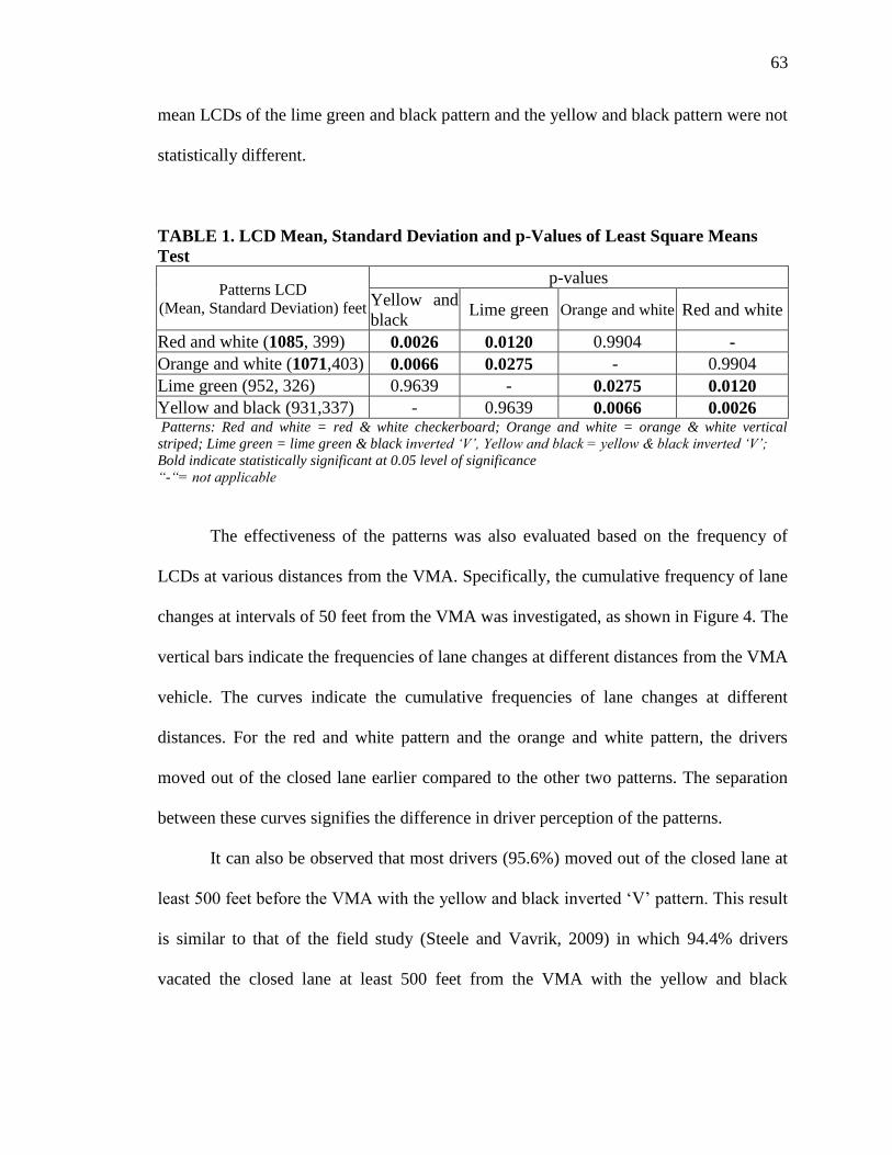
63
mean LCDs of the lime green and black pattern and the yellow and black pattern were not
statistically different.
TABLE 1. LCD Mean, Standard Deviation and p-Values of Least Square Means
Test
Patterns LCD
(Mean, Standard Deviation) feet
p-values
Yellow and
black Lime green Orange and white Red and white
Red and white (1085, 399) 0.0026 0.0120 0.9904 -
Orange and white (1071,403) 0.0066 0.0275 - 0.9904
Lime green (952, 326) 0.9639 - 0.0275 0.0120
Yellow and black (931,337) - 0.9639 0.0066 0.0026 Patterns: Red and white = red & white checkerboard; Orange and white = orange & white vertical
striped; Lime green = lime green & black inverted „V‟, Yellow and black = yellow & black inverted „V‟;
Bold indicate statistically significant at 0.05 level of significance
“-“= not applicable
The effectiveness of the patterns was also evaluated based on the frequency of
LCDs at various distances from the VMA. Specifically, the cumulative frequency of lane
changes at intervals of 50 feet from the VMA was investigated, as shown in Figure 4. The
vertical bars indicate the frequencies of lane changes at different distances from the VMA
vehicle. The curves indicate the cumulative frequencies of lane changes at different
distances. For the red and white pattern and the orange and white pattern, the drivers
moved out of the closed lane earlier compared to the other two patterns. The separation
between these curves signifies the difference in driver perception of the patterns.
It can also be observed that most drivers (95.6%) moved out of the closed lane at
least 500 feet before the VMA with the yellow and black inverted ‗V‘ pattern. This result
is similar to that of the field study (Steele and Vavrik, 2009) in which 94.4% drivers
vacated the closed lane at least 500 feet from the VMA with the yellow and black

64
inverted ‗V‘ pattern at a rural test site. This indicates similarities in the results of the
driving simulator and the field data.
FIGURE 4. Lane Change Distance Frequency and Cumulative Frequency Curves
for Different Patterns
The KS test for the LCD distributions of the red and white pattern with the lime
green and black pattern (p = 0.0048) and with the yellow and black pattern (p = 0.0007)
indicated that the distributions were not identical, the differences were statistically
significant, and the red and white pattern indicated higher cumulative frequency of lane
changes at the point of maximum separation between the distributions. The test for the
cumulative frequency distribution of the orange and white vertical striped pattern with the
lime green and black inverted ‗V‘ pattern (p = 0.0083) and with the yellow and black
inverted ‗V‘ pattern (p = 0.0014) also showed a significant difference in the cumulative
frequency of lane changes at the point of maximum separation between the distributions.
Therefore, the perceptions of drivers in response to the red and white checkerboard

65
pattern and the orange and white vertical striped pattern were statistically significant
compared to the lime green and black and the yellow and black inverted ‗V‘ patterns.
The driving simulator experiment demonstrated that when LCD is used as the
criterion, which is very important to avoid crashes with the VMA, the red and white
checkerboard pattern and the orange and white vertical striped pattern were most
effective, whereas the yellow and black inverted ‗V‘ pattern was the least effective.
4.2.2. Subjective Evaluation
The mean ranks of the patterns based on the four criteria are presented in Table 2.
To statistically test the participants‘ preferences of the patterns, PHREG analysis was
carried out with the yellow and black pattern as the base pattern. The yellow and black
pattern was used as the base pattern because it is the most widely used pattern in work
zones, especially in Missouri. Table 3 presents the results of the PHREG analysis. The
risk ratio from the analysis indicated the preferences of the participants for the patterns
when compared to the yellow and black pattern. The risk ratio for the yellow and black
pattern equaled 1.00. The patterns with values more than 1.00 were more preferred than
the yellow and black pattern. The patterns with risk ratios below 1.00 were less preferred
than the yellow and black pattern.
From the mean ranks in Table 2, the participants ranked the red and white
checkerboard pattern to be more visible (2.23), capturing more attention of drivers (2.15),
and contrasting better with the VMA truck (2.08) compared to the other patterns. For the
alerting drivers to work zones criterion, the yellow and black pattern had the lowest mean
rank (2.01) while the red and white checkerboard pattern had the highest mean rank

66
(2.95). This indicated that the yellow and black pattern is most effective in alerting
drivers to work zones; probably because it is the most commonly used pattern in work
zones.
TABLE 2. Mean Ranks for the VMA Patterns
Patterns/Criteria Visibility Alert drivers
to work zones
Capture attention
of drivers
Color
contrast*
Red and white 2.23 2.95 2.15 2.08
Orange and white 2.67 2.44 2.64 2.75
Lime green 2.55 2.60 2.58 2.34
Yellow and black 2.55 2.01 2.63 2.82 Patterns: Red and white = red & white checkerboard; Orange and white = orange & white vertical
striped; Lime green = lime green & black inverted „V‟, Yellow and black = yellow & black inverted „V‟;
Bold: Lowest mean value for the column, Underlined: Highest mean value for the column (Rank 1 =
highest, Rank 4 = lowest)
Color Contrast with the VMA vehicle
The risk ratios from the statistical analysis reported in Table 3 shows the odds of
selecting a given VMA pattern as the preferred pattern over the yellow and black base
pattern. For example, the risk ratio of 1.873 for the red and white pattern given under the
color contrast column indicated that the odds of the participants selecting the red and
white checkerboard pattern as the best was 87.3% higher than the selection odds for the
base pattern. Clearly the red and white pattern was preferred over the other patterns for
color contrast (risk ratio of 1.873 compared to 1.001, 1.439, and 1.0). This result was
statistically significant based on the p-value reported in Table 3. For the alerting drivers
to the work zones criterion, none of the patterns had a risk ratio that indicated that they
were preferred over the yellow and black pattern, with lime green and black pattern
having a risk ratio of 0.557, while the red and white pattern having the least risk ratio of
0.428. Both ratios were less than 1.0 indicating that the base pattern was preferred, and

67
the p-values for both patterns indicated that this preference was statistically significant.
The fact that the red and white pattern was least preferred for this criterion might be
because drivers have seldom been exposed to the red and white color pattern.
In a recent meeting, a MoDOT official explained that the red and white
checkerboard pattern will be implemented in work zones even though it is least able to
alert drivers and the results are expected to improve as drivers become familiar with the
pattern. From the mean ranks in Table 2, participants showed the least preference for the
yellow and black pattern (2.82) under the color contrast criterion with the VMA
background, probably because Missouri DOT VMA vehicles are yellowish orange in
color. Similar result was observed for the orange and white pattern.
TABLE 3. Risk Ratios and p-Values for the VMA Patterns
Patterns/Characteristics Visibility
Alert drivers
to work
zones
Capture
attention
of drivers
Color
contrast*
Red and white 1.310^
(0.1996)~
0.428
(<.0001)
1.487
(0.0601)
1.873
(0.0031)
Orange and white 0.9018
(0.6178)
0.668
(0.0549)
0.960
(0.8433)
1.001
(0.9961)
Lime green 0.993
(0.9726)
0.557
(0.0063)
1.033
(0.8737)
1.439
(0.0784)
Yellow and black 1.000
(-)
1.000
(-)
1.000
(-)
1.000
(-) Patterns: Red and white = red & white checkerboard; Orange and white = orange & white vertical
striped; Lime green = lime green & black inverted „V‟, Yellow and black = yellow & black inverted „V‟;
„-‟ indicates p-value not available for base pattern,
Bold font indicates statistically significant at 0.05 level
* Color Contrast with the VMA vehicle
When the participants were asked which pattern was most preferred, 27 drivers
(36.98%) preferred the red and white checkerboard pattern, 19 (26.02%) preferred the
lime green and black inverted ‗V‘ pattern, 15 (20.5%) preferred the yellow and black

68
inverted ‗V‘ pattern, and 12 (16.4%) preferred the orange and white vertical stripes
pattern. Thus, the red and white checkerboard pattern was found to be the most preferred
pattern among the four.
Table 4 presents the mean ranks when the drivers were surveyed about the
different features of each pattern. This part of the subjective survey was different
compared to the mean ranks presented in Table 2 in which the four patterns were ranked.
Table 4 presents the mean ranks of the features of each pattern. This was carried out
mainly to identify the features that are distinct for each VMA marking. Table 4 indicates
that the drivers preferred the inverted ‗V‘ pattern design for the lime green and black
pattern and the yellow and black pattern. For the lime green and black pattern, the least
liked feature was the color combination. Color contrast was most liked for the red and
white checkerboard pattern and least liked for the yellow and black inverted ‗V‘ pattern.
For the orange and white striped pattern, the color combination was the most liked
feature and color contrast was the least liked feature.
TABLE 4. Mean Ranks of the Features for the VMA Patterns
Features \ Patterns Red and white Orange and white Lime green Yellow and
black
Pattern Design 2.07 2.01 1.81 1.89
Color Combination 2.11 1.95 2.18 1.91
Color Contrast* 1.82 2.04 2.01 2.21 Patterns: Red and white = red & white checkerboard; Orange and white = orange & white vertical
striped; Lime green = lime green & black inverted „V‟, Yellow and black = yellow & black inverted „V‟;
Bold: Lowest mean value for the column, Underlined: Highest mean value for the column (Rank 1 =
highest, Rank 3 = lowest)
*Color Contrast between the different colors of the pattern
The post-experiment survey yielded some interesting results. Based on
discussions with representatives of Missouri DOT, the inverted ‗V‘ pattern was

69
considered an effective sign for drivers to change lanes in a specific direction and to
move out of the closed lane. Further, the checkerboard pattern was expected to indicate
clearly a lane closure without indicating the direction of lane change. However, when
participants were surveyed regarding the information provided by the inverted ‗V‘
pattern, 57 (78%) did not perceive that the inverted ‗V‘ design signifies the direction of
lane change, and only 16 (22%) perceived that it signifies a lane change either to the left
or to the right. Regarding the checkerboard pattern, 41 (56%) participants stated that it
indicates a need to reduce speed, 16 (22%) stated that it indicates a need to stop, and an
equal number stated that it conveys no message.
5. CONCLUSIONS AND RECOMMENDATIONS
This paper presents the results of a survey of state DOTs and a driving simulator
study to evaluate the perception of younger drivers for striping patterns and color
combinations for VMAs used in work zones during the daytime. Out of the 30 state
agencies that responded to the survey, it was found that 22 (77%) use VMAs in work
zones to meet the requirements of transportation agency policy and one agency uses
VMAs to meet the requirements of state law. The yellow and black inverted ‗V‘ pattern
was most commonly used by DOTs as it is provided by the VMA suppliers.
The driving simulator study evaluated the VMA markings using objective and
subjective evaluation criteria. The objective evaluation used LCD as the criterion. It can
be inferred from the LCDs that the red and white checkerboard pattern and the orange
and white vertical stripes pattern were more effective compared to the two other patterns
evaluated. The results of the subjective evaluation indicated that the red and white

70
checkerboard pattern was ranked highest for visibility, color contrast, and capturing the
attention of drivers. The participants regarded the yellow and black inverted ‗V‘ pattern
as highly effective in alerting drivers to a work zone.
Thus, out of the four VMA patterns evaluated, the red and white checkerboard
was found to be more effective and preferred overall than the other patterns. Further
evaluations are being conducted with older drivers and during dusk and nighttime
conditions. VMA patterns should also be evaluated based on differences in heights,
flashing patterns of arrows and beacons, and use in different work zone configurations.
Further, crash data should be used to evaluate the effectiveness of VMAs.
ACKNOWLEDGEMENTS
The authors gratefully acknowledge the grants for this project from the Smart
Work Zone Deployment Initiative, the Mid-America Transportation Center, and the
Intelligent Systems Center at the Missouri University of Science and Technology.
REFERENCES
Allison, P. D. and Christakis, N. A. (1994). Logit Models for Sets of Ranked Items, in
Sociological Methodology, ed. P.V. Marsden, Oxford: Basil Blackwell, 199-228.
American Association of State Highway and Transportation Officials (2002), Roadside
Design Guide, Washington, D.C.

71
Atchley, P. (2006). ―The effect of fluorescent yellow-green background for vehicle-
mounted work zone signs on attention and eye movements.‖ FHWA,
<http://www.ctre.iastate.edu/smartwz/reports/2006_atchley_fygborder.pdf>.
Bham, G. H., Leu, M. C., Mathur, D. R., and Javvadi B. S. (2009). ―Evaluation of
Vehicle Mounted Attenuator (VMA) Markings Using a Driving Simulator for Work
Zones.‖ Proc., the 88th
Annual Meeting of the Transportation Research Board, January
2009, Washington, D.C.
Crash Data. (2007). Brian Chandler, Safety Engineer formerly with the Missouri
Department of Transportation.
Fatality Analysis Reporting System. (FARS) (2010).
<www.fars.nhtsa.dot.gov/Main/index.aspx> (Jan. 22, 2010).
Humphreys, J. B. and Sullivan, T. D. (1991). ―Guidelines for the Use of Truck-Mounted
Attenuators in Work Zones.‖ Transportation Research Record. 1304, 292-302.
Kamyab, A., and Storm B. (2001). ―FYG backing for work zone signs.‖ FHWA Pooled
Fund Study. Report.
Kramer, C. Y. (1956). ―Extension of Multiple Range Tests to Group Means with Unequal
Sample Sizes.‖ Biometrics. 12, 307-310.

72
Mackay, R. G., and John L. P. (1995). ―Experience with Truck Mounted Attenuators.‖
Public works. 1995, Vol. 126, No. 11, 44.
Manual on Uniform Traffic Control Devices (2003). U.S. Department of Transportation.
Federal Highway Administration. Washington D.C.
National Work Zone Safety Information Clearinghouse (NWZSIC) (2010).
< http://www.workzonesafety.org/crash_data/workzone_fatalities> (Feb. 21st, 2010)
SAS/STAT 9.2 User‘s Guide (2008). SAS Institute Inc.
Smith, J., Edwards, R., O‘Neil, S., and Goluchowski, M. (2006). ―Best practice for use
and design of truck mounted attenuators (TMA) for New Zealand roads.” Land
Transport New Zealand Research. Report 301, 100.
Steele, D. A., and Vavrik, W. R. (2009). ―Improving the Safety of Moving Lane
Closures.‖ Illinois Center for Transportation. ICT-R37-32.
Wang, Y., Zhang, E. D., Zhang, W., Leu, M. C., and Zeng, H. (2006). ―Development of a
Low-cost Driving Simulation System for Safety Study and Training.‖ Proc. of the
Driving Simulation Conference-Asia/Pacific, Tsukuba, Japan, May 31-Jun. 2.

73
3. A DRIVING SIMULATOR STUDY:
EVALUATION OF VEHICLE MOUNTED ATTENUATOR MARKINGS IN
WORK ZONES DURING DIFFERENT TIMES OF THE DAY
Ghulam H. Bham1, Ming C. Leu
2, Durga Raj Mathur
2, V. A. Samaranayake
3, Manoj
Vallati2
Civil, Architecture and Environmental Engineering1
Mechanical and Aerospace Engineering2
Mathematics and Statistics3
Missouri University of Science and Technology (Missouri S&T)
ABSTRACT
This paper presents a study of driver perceptions using a driving simulator carried
out on the effectiveness of four markings, which vary in striping patterns and color
combinations, used at the rear of vehicle mounted attenuators (VMAs) in work zones
during daytime, dusk and nighttime. One hundred and twenty participants from different
age groups took part in the evaluation of VMA markings by driving through virtual
highway work zones. During this experiment, driver reaction to VMA markings was
determined based on their lane change distance (LCD). Additionally, the drivers were
surveyed using a detailed subjective survey. Analysis of variance (ANOVA) was
performed to determine the significant variables affecting the LCD. For each time of day,
a pair wise least-square means test was conducted to calculate the difference in LCD
between the markings. A Kolmogorov-Smirnov test was carried out to evaluate the
significance of differences between the LCD frequency distributions of the markings. For
the subjective evaluation, the markings were ranked by participants indicating their
preferences using four different criteria for each time of day. The participants were also

74
surveyed on the features of the individual markings and for the most preferred marking.
The results of the objective and subjective evaluations indicated that, overall, the red and
white checkerboard pattern was most effective.
Key words: vehicle mounted attenuator (VMA), driving simulator, virtual reality, work
zone, driver behavior, traffic control device (TCD), state department of transportation
1. INTRODUCTION
Work zone safety is a high priority for transportation agencies and the highway
construction industry because of the high frequency of work zone fatalities. The number
of such fatalities grew in the United States by nearly 45% between 1997 and 2006, from
693 to 1004 (NWZSIC, 2010). The safety of construction operations has received much
attention over the past several years. As crash frequency continues to increase, mostly
due to increase in highway construction activities, preventing crashes and reducing the
severity of crashes require anticipation of driver reactions to specific situations, which is
addressed in this paper.
Vehicle mounted attenuators (VMAs) are crash cushions mounted at the rear of
vehicles and can reduce the severity of rear-end collisions with construction vehicles in
work zones. Humphrey and Sullivan (1991) studied the effectiveness of VMAs and
indicated that these devices save about $23,000 per crash and reduce damage to the
construction vehicle. The study also showed that injury rates were higher when
construction vehicles were not equipped with VMAs. Safety improvements generally can
adopt one of two approaches. The first approach focuses on protecting vehicle occupants

75
in the event of a crash whereas the second approach focuses on preventing crashes. The
present study addresses the second approach.
The Manual on Uniform Traffic Control Devices (MUTCD) (2003) and the
American Association of State Highway and Transportation Officials (AASHTO)
Roadside Design Guide (2002) both contain general guidelines for VMAs. Neither
publication, however, includes recommendations for striping patterns and/or colors for
these devices. The predominant color combinations used by the state Departments of
Transportation (DOTs) are yellow and black, orange and white, red and white, and lime
green and black in an inverted ‗V‘, striped or checkerboard design. Figure 1 shows
striping patterns and color combinations mainly used by the DOTs in the United States.
(a) Lime Green and Black Inverted ‗V‘ Pattern (b) Red and White Checkerboard Pattern
(c)Yellow and Black Inverted ‗V‘ Pattern (d) Orange and White Vertical Stripes Pattern
FIGURE 1. Vehicle Mounted Attenuator Patterns
This study evaluates the driver perception of the effectiveness of various striping
patterns and color combinations for VMAs. Of particular concern is the use of an
inverted ‗V‘ design when the following vehicles do not have the option of passing on

76
either side of the work vehicle. The importance of contrast with the truck/vehicle color is
also of interest. The results of this study can help state DOTs to select the most effective
VMA color combination and striping pattern, thereby contributing to the improvement of
safety and operations in work zones on high-speed, high-volume roadways.
Driver perception and behavior can be evaluated by field studies, traffic modeling
and simulation, and using a driving simulator. Popular microscopic traffic simulation
models do not incorporate driver perceptions such as vision, hearing, driver sight
identification distance and cannot be used to evaluate the colors and patterns of traffic
control devices (TCDs). Field data collection can test a limited number of TCDs. Driving
simulator studies, however, permit the study of hazardous driving situations that cannot
be safely replicated during field tests. Such studies can be efficient and facilitate the
collection of a wide range of data. They are also repeatable, and permit easy and safe
replication of numerous scenarios to evaluate subjects‘ reaction to multiple TCDs.
A field study carried out on VMAs in New Zealand (Smith, Edwards, O‘Neil, and
Goluchowski, 2006) reported that flashing strobe lights provided enhanced capabilities
over rotating beacons, with at least 11.3% of drivers reacting at distances larger than 984
feet during nighttime. Under day and night conditions, a wide retro-reflective tape around
the edges of the arrow board significantly improved drivers‘ average recognition distance
of the VMA by at least 125 feet. Also, the recognition distance increased at night when
the traffic volumes were lower (i.e. approximately 400 vehicles/hour) as compared to
recognition distance during the day with higher traffic volumes (i.e. approximately 880
vehicles/hour). The drivers were not observing the far-distance ahead probably because

77
they were more focused on monitoring the activities of other drivers who may be a
potential risk to them.
Another field study on driver behavior (Steele and Vavrik, 2009), aimed at
improving the safety of moving lane closures found that 94.4% of drivers moved out of
the closed lane at more than 500 feet before the start of the taper for a rural test site
compared to 86.8% for an urban area. The percentage of vehicles that reached the VMA
vehicle within 500 feet was 4.8% and 12.2% for rural and urban areas, respectively.
Studies have also compared the use of different colors. Kamyab and Storm (2001)
used a fluorescent yellow-green background with an orange sign and found that this
showed an improvement in the contrast between the sign and the orange DOT truck.
They conducted a driver survey on the visibility of the sign with and without the
fluorescent background. Traffic volumes were measured and data analysis revealed
significant decrease in traffic volume within 100 feet for the lane where the truck was
present when the fluorescent yellow-green background was used with the sign. Another
study by Atchley (2006), however, suggested that fluorescent traffic signs have no
advantage over non-fluorescent signs.
The literature reviewed did not offer specific guidelines for selecting VMA color
combinations or striping patterns. The present research is a first step towards determining
effective VMA markings for use in construction zones for different times of the day with
drivers from different age groups.

78
2. METHODOLOGY
A driving simulator was used to evaluate driver perceptions and behavior
objectively as well as subjectively. This section presents the driving simulator
experimental setup, the statistical data analysis to evaluate the objective and subjective
data and the details of the questionnaires used.
2.1. Missouri S&T Driving Simulator
A fixed-base driving simulator used for this study comprised of a passenger car,
three LCD projectors, a projection screen, and three networked computers with Ethernet
connection. The computer that processes the vehicle movements was defined as the
master; the other two computers were defined as slaves. The passenger car is a Ford
Ranger pick-up truck with a speedometer, and different types of optical sensors are used
to measure the steering operation, vehicle position, speed, acceleration/deceleration, and
braking. The screen has an arc angle of 54.6°, an arc width of 25 feet and a height of 6.6
feet. The field of view is around 120°.
The resolution of the visual scene generated by the master was 1024×768 pixels,
and that for the slaves was 800×1200 pixels; the refresh rate was 30 to 60 Hertz
depending on the scene complexity. The system was also equipped to reproduce engine
sound. A more detailed description of the system structure, projection system, and the
data acquisition process can be found in Wang et al. (2006).

79
2.2. Work Zone Setup and Configuration
Work zone scenarios for daytime, dusk and nighttime were developed which
replicated a 4-lane rural divided highway. Each scenario included four consecutive work
zones on a highway with different VMA markings. The highway was approximately
eight miles long; first work zone was setup after 1.5 miles, each work zone was 0.5 miles
long and 1.5 miles apart. Figure 2 shows a work zone setup with traffic control devices,
two VMA vehicles (with the same markings), and a construction vehicle on the closed
lane. The four VMA markings varied randomly for the participants driving on the virtual
highway with work zones.
FIGURE 2. Work Zone Configuration
The virtual work zone environment created for the experiment was set up
according to MUTCD (2003) and Missouri DOT specifications for a partial lane closure
on a divided highway. These guidelines specified sign spacings, taper lengths, and

80
optional buffer length channelizer spacings for various speed limits, sign heights, and
work zone lengths. To replicate a real environment, traffic control devices such as cones,
barriers, and traffic signs were placed on the highway. The first 1.5 miles of the freeway
had a speed limit of 70 mph indicated by a regulatory speed limit sign at the beginning of
the section. Additional traffic signs were placed along the right side of the roadway 500
feet apart, as shown in Figure 2, starting with ‗Road Work Ahead‘ warning sign located
1.5 miles at the start of the work zone. The four remaining signs were placed in the
following order: speed limit sign ‗45 mph‘, ‗Right Lane Closed Ahead,‘ another speed
limit sign ‗45 mph,‘ and then ‗Right Lane Closed Ahead‘ again. Each construction zone
was 1300 feet in long with barriers on the lane markings. The construction zone consisted
of a shadow vehicle with a VMA, a work vehicle with a VMA, and a construction
vehicle. These vehicles were separated by a distance of 550 feet.
2.3. Participants
Participants in this study were students, staff and faculty from Missouri S&T, and
residents of Rolla, Missouri. One hundred and twenty people were selected to participate
in the experiment. Three age categories were selected for this study: younger aged group
was 18 to 34 years (sample size (S) = 70, mean (M) = 21.8 years, standard deviation (SD) =
2.0 years), middle aged group was 35 to 64 years (S = 30, M = 45.3, SD = 7.6), and older
aged group 65 years and up (S = 20, M = 73.3, SD = 6.8). The gender split was
approximately 50/50 for all age groups. Prior to scheduling the experiment, the participants
were screened using a questionnaire to inquire if they have a US driver‘s license, any
health issues that would affect driving, and they do not suffer from motion sickness. All
participants had normal or corrected-to-normal vision and none of them reported any

81
form of color deficiency. Most surveyed met the requirements and participated in the
experiment. Of the 120 participants, 51 had been driving for more than 15 years, 49 had
been driving between 5 and 15 years, and 20 had been driving between 1 and 5 years. All
participants had previously encountered VMAs in highway work zones.
2.4. Experiment
Before the start of the experiment, the participants were checked if they were
carrying a valid US driving license with them. Participants who were found without a
valid US license were turned away from the experiment. The participants were first given
a brief introduction to the driving simulator and advised to adhere to traffic laws and to
drive as they would in normal traffic conditions. The participants were also notified that
they could quit the experiment at any time in case of motion sickness or discomfort. To
familiarize the participants with the driving simulator, the environment, and the
instructions, the participants first drove through a trial scenario similar to that used in the
experiment. Typically, each participant first drove for several minutes during the trial
run. After the trial run, each subject drove through the three scenarios: daytime, dusk and
nighttime in random order. Also, the four work zones with different VMA patterns
appeared in random order and were equally distributed within each scenario. Driver
behavior data was collected by various sensors of the driving simulator for every 0.1
seconds.
The markings used in the present study did not incorporate retro-reflective
properties. During a visit to Missouri DOT‘s maintenance facility, it was observed that
the yellow and black inverted ‗V‘ pattern did not have retro-reflective properties whereas

82
the red and white checkered board pattern newly bought by the DOT had retro-reflective
markings.
2.5. Pre- and Post-Experiment Questionnaires
All participants were surveyed before and after the driving simulator experiment.
The pre-experiment questionnaire inquired about any health issues and consumption of
alcohol/drug use during the last 24 hours of the experiment. This was carried out to
ensure that drivers were alert and eligible for participation on the day of the experiment.
After the driving simulator experiment, each participant was asked to complete a
post-experiment questionnaire. The questionnaire served as the subjective evaluation of
the VMA patterns based on the participant‘s experience with the driving simulator. The
participants were asked to rank the four patterns based on the following criteria: i)
visibility, ii) alerting drivers to work zones, iii) capturing the attention of drivers, and iv)
color contrast with the VMA vehicle, by different times of the day. Visibility was used as
a criterion for evaluation of the VMAs because it is important with regard to specific
conditions such as times of the day and the environment. A VMA pattern that is visible
from a distance would alert the drivers to construction activity downstream, thus reducing
the risk of a crash. The pattern that captures the attention of the drivers would cause them
to notice a work zone and change lanes before approaching the VMA. Alerting drivers to
work zones and contrast with the VMA background were used as criteria to make
conclusions about the best possible color combinations that contrast with the construction
equipment.

83
The participants were also asked to rank features of individual striping patterns
they liked the most. This was carried out to indicate their preference for each marking
based on pattern design, color combination, and color contrast using a scale of 1 to 3,
with 1 indicating most liked and 3 indicating least liked. The participants were also asked
to indicate their overall preference of a pattern and how they interpreted the meaning of
some of the features of the markings.
2.6. Data Analysis
The drivers‘ acceleration/deceleration, speed, position and steering angle were the
main variables measured during the driving simulator experiment, for use in the objective
evaluation. From vehicle positions, the distances from the point of lane change to the
VMA on the closed lane were obtained. This distance, called the lane change distance
(LCD), was used as a criterion for determining the effectiveness of the VMA patterns.
The LCD was measured from the point where the driver began to steer continuously out
of the right lane towards the left lane, achieving the maximum steering angle. The drivers
were assumed to be responding to the appearance of the VMA pattern in the construction
zone. LCD was selected because most DOTs that responded to a survey (Bham et al.,
2009) conducted as part of this study, indicated its use to determine the effectiveness of
VMAs in work zones. The details of the state DOT survey and the results have been
presented elsewhere (Bham et al., 2009) and thus are not repeated here. Further, the study
(Bham et al., 2009) found that the speed-reduction identification distance, i.e. the
distance from the VMA at which the drivers start decelerating, should not be used to

84
evaluate VMA patterns because drivers reduce their speed in response to advance
warning signs.
The driving simulator experiment was set up such that each participant drove
through the three scenarios: daytime, dusk and nighttime in random order. During each
scenario the drivers were exposed to the four VMA markings in random order as well.
The appropriate statistical design for this experiment was a split-split-plot, with each
participant represented as a main-plot with gender and age group playing the role of
main-plot factors, the time-of-day acting as the sub-plot factor and the four markings as
the sub-sub-plot factor. The aggregate data was unbalanced because the numbers of
participants tested for each marking and time-of-day combination were different. This
was caused by drivers who did not complete the experiment as they had to leave and the
result of data loss due to human error.
Analysis of variance (ANOVA) was carried out to test the statistical significance
of gender, age groups, time-of-day, VMA markings, and their interactions on the mean
LCD. The test was conducted using the Statistical Analysis System (SAS, 2008) software
package. The statistical significance (null hypothesis) of independent variables (factor) or
the interactions of two or more variables on the mean LCD was rejected if the p-value
was less than or equal to the chosen significance level of 0.05. Because of the unbalanced
data, the expected mean squares for the error terms (three error terms in a split-split-plot
setup: the main-plot error, the sub-plot error, and the sub-sub-plot error) and those for the
corresponding treatment effects did not match exactly under the null hypothesis. As a
result of this, each test was carried out manually by computing the error terms for each
test based on the estimates of the three variance components associated with the main-

85
plot, sub-plot and sub-sub-plot error terms. The error terms were constructed such that
under the null hypothesis the tested effect is zero, the expected mean squares of the tested
effect and the corresponding error terms are equal.
Pairwise comparisons of least-square means (LSM) between patterns for each
time of day were performed in SAS software. LSM are predicted values, based on the
model fitted, across values of a categorical effect where other model factors are held
constant by setting them to the least square estimate of their mean. If the experiment is
balanced where each combination of factors (i.e., independent variables) is replicated an
equal number of times, least square means will be the same as regular sample means. In
this experiment, however, equal samples were not available within the factor
combinations, therefore, sample means were not unbiased estimates of the true
population means associated with the treatment combinations and the use of the least-
square means was warranted. The least-square means test was conducted by employing
the Tukey-Kramer adjustment, which uses the approximation described by Kramer
(1956). It was used to accommodate the unbalanced data and provide good control of the
Type 1 error rate.
To further analyze the data, a Kolmogorov-Smirnov (KS) test was also conducted
for each time of day to ascertain statistically significant difference between the lane-
change cumulative frequency distributions for the four VMA patterns. The KS procedure
tests the null hypothesis of no significant difference between the LCD cumulative
distributions for the four VMA markings by looking at the difference at the point of
maximum separation between the distribution curves. This is in contrast to the ANOVA
based test described earlier, which looked at the differences between the means. A
86
significant difference between the frequency distributions for any two markings for a
given time of day would imply that the lane-change behavior of drivers was different
between these markings. Straightforward use of the KS test on the LCD distribution of
participants would reduce the power of the test because of the heterogeneity of
participants‘ driving styles and would add to the ―noise‖ in the data. The effect of an
individual participant‘s driving style was eliminated by calculating the dependent
variable as the difference between the marking LCD for a participant and the average
LCD of that participant for the four markings. This distance was used instead of the
actual LCD of the marking for the KS test. The KS test was conducted at 0.05 level of
significance.
To supplement the objective evaluation, all participants completed a post-
experiment questionnaire for subjective evaluation of the VMA markings. The subjective
evaluation served as an opinion poll of the participants regarding the four markings in
contrast with measuring the effect of the marking on the actual driving behavior. The
results of the subjective evaluation should be carefully interpreted as they represent the
perception of the drivers. The analysis of the subjective evaluation was carried out for
each time of day as it was found from the objective evaluation that the subjects reacted
differently to the patterns at different times of the day. Thus, the mean rank for a
particular pattern was calculated by taking the arithmetic mean of the ranks for each time
of the day and for each criterion.
A statistical test was also carried out to find the significance of participants‘
preference of the markings. It should be noted here that the participants did not choose a
preferred marking from among the four but ranked them according to a criterion. Thus,

87
the data from an individual provides information on his/her ranked preference as the first,
second, third and the last choice. Further, the ranks for each marking were correlated for
an individual. The statistical model that was used to analyze this data can be explained as:
first, a participant selected his/her the first choice (rank = 1, the highest rank). Then,
among the rest, the next best choice was selected (rank = 2) and so on. The resulting
model is sometimes referred to as the exploded logit model, a discussion of which can be
found in Allison and Christakis (1994). The likelihood function obtained for this model is
exactly the same as the likelihood one would obtain for the stratified Cox regression
analysis and thus can be estimated using the PHREG procedure in SAS (2008). In this
context, the PHREG procedure estimates the parameters of the model and provides risk
ratios of proportions, which are the odds of a marking to be ranked 1 (best) under a
particular criterion when compared against a base marking. For analysis of results, the
yellow and black inverted ‗V‘ pattern was used as the base pattern and the risk ratios for
the rest of the markings with respect to it were estimated.
3. ANALYSIS OF RESULTS
3.1. Objective Evaluation
Table 1 presents the results of the split-split-plot ANOVA test. The analysis
indicated that the variables: Gender, Age group, and the interaction term Time-of-
day*Pattern were statistically significant. Age group and Gender showed no significant
interaction with other variables or with each other. Their effects on the LCD were,
therefore, not evaluated individually. The time-of-day and pattern were evaluated
individually because they had significant interaction in their effects on the LCD.

88
The data showed that the average LCD for the older age group for all the markings
and times of the day, 1058 feet and this was greater than the LCD of the younger age group
drivers, 854 feet, and the middle age group drivers, 847 feet. This shows that the older
drivers moved out of the closed lane much earlier than the younger and the middle age
drivers. The difference in LCD clearly indicates that older drivers were risk averse and
perhaps less prone to colliding with the VMA.
TABLE 1. Statistical Results: Main Effects and Interactions
Source DFNUM# DFDEN^ F-ratio Prob > F
Gender 1 114 4.30 0.0403
Age group 2 114 6.44 0.0022
Gender*Age group 2 114 0.47 0.6233
Time of day 2 220 105.12 <0.0001
Gender*Time of day 2 220 0.59 0.5516
Time of day*Age group 4 220 1.48 0.2070
Gender*Time of day*Age group 4 220 2.40 0.0507
Pattern 3 982 14.59 <0.0001
Gender*Pattern 3 982 1.77 0.1516
Age group*Pattern 6 982 1.55 0.1595
Gender*Age group*Pattern 6 982 0.70 0.6473
Time of day*Pattern 6 982 3.18 0.0043
Gender*Time of day*Pattern 6 982 0.72 0.6343
Time of day*Age group*Pattern 12 982 0.74 0.7144
Gender*Time of day*Age
group*Pattern
12 982 0.73 0.7199
# DFNUM = (Number of different groups – 1)
^DFDEN = (Total sample size) – (Number of different groups)
The interaction between Age group and Pattern was not significant, indicating that
the order of effectiveness of the markings was similar in all the age groups. It was also found
that the mean LCD for male drivers (848 feet) averaged over all times of the day was shorter
than that for female drivers (924 feet). Clearly, female drivers moved out of the closed lane
earlier than the male drivers, suggesting that the male drivers were aggressive and more
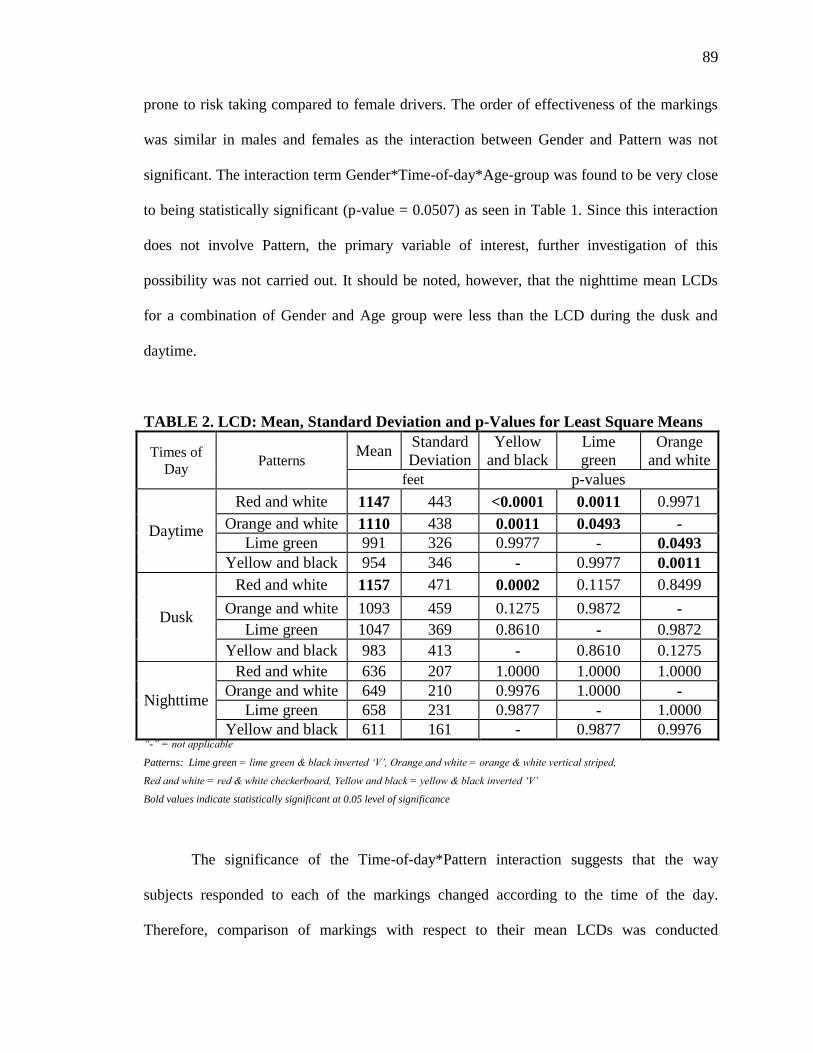
89
prone to risk taking compared to female drivers. The order of effectiveness of the markings
was similar in males and females as the interaction between Gender and Pattern was not
significant. The interaction term Gender*Time-of-day*Age-group was found to be very close
to being statistically significant (p-value = 0.0507) as seen in Table 1. Since this interaction
does not involve Pattern, the primary variable of interest, further investigation of this
possibility was not carried out. It should be noted, however, that the nighttime mean LCDs
for a combination of Gender and Age group were less than the LCD during the dusk and
daytime.
TABLE 2. LCD: Mean, Standard Deviation and p-Values for Least Square Means
Times of
Day Patterns
Mean Standard
Deviation
Yellow
and black
Lime
green
Orange
and white
feet p-values
Daytime
Red and white 1147 443 <0.0001 0.0011 0.9971
Orange and white 1110 438 0.0011 0.0493 -
Lime green 991 326 0.9977 - 0.0493
Yellow and black 954 346 - 0.9977 0.0011
Dusk
Red and white 1157 471 0.0002 0.1157 0.8499
Orange and white 1093 459 0.1275 0.9872 -
Lime green 1047 369 0.8610 - 0.9872
Yellow and black 983 413 - 0.8610 0.1275
Nighttime
Red and white 636 207 1.0000 1.0000 1.0000
Orange and white 649 210 0.9976 1.0000 -
Lime green 658 231 0.9877 - 1.0000
Yellow and black 611 161 - 0.9877 0.9976 “-” = not applicable
Patterns: Lime green = lime green & black inverted „V‟, Orange and white = orange & white vertical striped,
Red and white = red & white checkerboard, Yellow and black = yellow & black inverted „V‟
Bold values indicate statistically significant at 0.05 level of significance
The significance of the Time-of-day*Pattern interaction suggests that the way
subjects responded to each of the markings changed according to the time of the day.
Therefore, comparison of markings with respect to their mean LCDs was conducted

90
separately for each time of day. Table 2 summarizes the mean and standard deviation of LCD
for the four markings for each time of the day. Further statistical analysis was conducted to
find which markings were significantly different from the others within each time-of-day
category. A KS test was also performed to determine if there was a significant difference
between the frequency distribution of the LCD associated with each of the markings. The
results below are categorized by time of day so they are easier to comprehend.
3.1.1. Daytime Conditions
From Table 2, for daytime conditions, on average, drivers changed the lane
farthest from the work zone when the red and white pattern, 1147 feet, and the orange
and white pattern, 1110 feet, were used on the VMA. For the lime green and black
pattern, drivers changed lanes on an average of 991 feet from the VMA. The mean LCD
of 954 feet for the yellow and black pattern was the lowest.
As stated earlier, the differences between the mean LCD of markings during
different times of the day were tested for significance using the least square means. The
mean LCD of the red and white pattern was found to be significantly higher than that of
the lime green and black pattern and the yellow and black pattern. Similarly, the mean
LCD of the orange and white pattern was also significantly greater than that of the lime
green and black pattern and the yellow and black pattern. The difference between the
mean LCD of the red and white pattern and the orange and white pattern was not found to
be statistically significant. Similarly, the difference in mean LCD between the lime green
and black pattern and the yellow and black pattern was not significantly different. Thus,
the mean LCDs for the red and white checkerboard and the orange and white vertical
striped patterns were significantly larger than those of the other patterns for daytime.

91
The effectiveness of the markings was also evaluated based on the cumulative
lane change frequency, represented by curves in Figure 3, at intervals of 50 feet from the
VMA. An interval of 50 feet was reasonably long to evaluate the difference in the
frequency distributions. Figure 3 also indicates the observed frequency and percentage of
drivers changing lanes at various distances from the VMA. Most drivers, 95.6%, moved
out of the closed lane at least 500 feet from the VMA when the yellow and black inverted
‗V‘ pattern was used. This result is similar to that of a field study (Steele and Vavrik,
2009) in which 94.4% drivers changed their lane at least 500 feet from the VMA with the
yellow and black inverted ‗V‘ pattern used at a rural test site in Illinois. This indicates
similarities in the results from the driving simulator and from the field data.
The KS test for the LCD distributions of the red and white pattern with the lime
green and black pattern (p < 0.0001) and with the yellow and black pattern (p < 0.0001)
indicated that these distributions were not identical and the differences were statistically
significant at the point of maximum separation. Table 3 presents the results of the KS
test. In these cases, the red and white checkerboard pattern had higher cumulative
frequency of lane changes at the point of maximum vertical separation between the
distributions. The test of the cumulative frequency distributions of the orange and white
vertical striped pattern with the lime green and black inverted ‗V‘ pattern (p < 0.0001),
and with the yellow and black inverted ‗V‘ pattern (p < 0.0001) also showed a
statistically significant difference. This indicates that the driver perceptions in response to
the red and white checkerboard pattern and the orange and white vertical striped pattern
were significantly better compared to the lime green and black and the yellow and black
inverted ‗V‘ patterns.

92
(a) Daytime
(b) Dusk
(c) Nighttime
FIGURE 3. Lane Change Distance Frequency Histogram and Cumulative
Frequency Curves for Different Times of the Day

93
3.1.2. Dusk Conditions
From Table 2, for dusk conditions, the mean LCDs showed the same trend
observed for daytime conditions. The results of the LSM test indicated that there was no
significant difference between the mean LCDs of the patterns except that the mean LCD
of the red and white checkered board pattern was significantly (p = 0.002) greater than
the mean LCD of the yellow and black inverted ‗V‘ pattern.
TABLE 3. Kolmogorov-Smirnov Test Results
Times of
Day Patterns
Yellow
and black Lime green
Orange and
white
p-values
Daytime
Red and white <.0001 <.0001 0.8824
Orange and white <.0001 <.0001 -
Lime green 0.2961 - -
Yellow and black -
Dusk
Red and white <.0001 0.0209 0.4600
Orange and white <.0001 0.2867 -
Lime green 0.0209 - -
Yellow and black -
Nighttime
Red and white 0.7905 0.0674 0.2281
Orange and white 0.0476 0.0010 -
Lime green 0.1726 - -
Yellow and black - “-” = not applicable
Patterns: Lime green = lime green & black inverted „V‟, Orange and white = orange & white vertical striped,
Red and white = red & white checkerboard, Yellow and black = yellow & black inverted „V‟
Bold values indicate statistically significant at 0.05 level of significance
From Figure 3(b), it can be observed that most of the drivers recognized the
construction zone from a distance of more than 400 feet. This can be attributed to better
color contrast with the surroundings during dusk conditions. The KS test, Table 3, for the
LCD distributions of the red and white pattern with the lime green and black pattern (p =
0.0209) and with the yellow and black pattern (p < 0.0001) indicated that the

94
distributions were not identical at the point of maximum separation. For these cases, the
red and white checkerboard pattern had a higher cumulative frequency of lane changes at
the point of maximum vertical separation. The test of cumulative frequency distributions
of the yellow and black inverted ‗V‘ pattern with respect to the lime green and black
inverted ‗V‘ pattern (p = 0.0209) and to the orange and white vertical striped pattern (p <
0.0001) also showed a significant difference with a lower cumulative frequency of lane
changes for the yellow and black inverted ‗V‘ pattern at the point of maximum
separation. Therefore, driver perception in response to the red and white checkerboard
pattern, the orange and white vertical striped pattern, and the lime green and black
inverted ‗V‘ pattern was better compared to the yellow and black inverted ‗V‘ pattern.
3.1.3. Nighttime Conditions
It can be observed from Table 2 that the mean LCDs for the four markings were
very similar. No significant difference between the mean LCDs for the four markings was
observed.
3.2. Subjective Evaluation
The participant‘s preferences indicated by mean ranks of the markings based on
the four criteria are presented in Table 4. To statistically test these preferences, statistical
analysis was carried out with the yellow and black pattern as the base pattern. The yellow
and black pattern was used because it is the most widely used pattern in work zones
especially in Missouri. Table 5 presents the results of the statistical analysis. The risk
ratio indicated the participants‘ preferences of the markings when compared to the yellow
95
and black pattern. The risk ratio for the yellow and black pattern equaled 1.0. The
markings with values more than 1.0 were preferred over the yellow and black pattern.
Conversely, the markings with risk ratios below 1.0 were less preferred than the yellow
and black pattern.
3.2.1. Daytime Conditions
From the mean ranks in Table 4, the participants ranked the red and white
checkerboard pattern to be more visible (2.14), captured the attention of drivers (2.09),
and contrasted better with the VMA vehicle (1.96) in comparison to the other markings.
For the alerting drivers to work zones criterion, the yellow and black pattern had the
lowest mean rank (1.98), which indicated that participants found it highly effective. The
red and white checkerboard pattern had the highest mean rank (2.87), ranking it as the
least effective in alerting drivers to work zones. The risk ratios from the statistical
analysis reported in Table 5 shows the odds of selecting a given VMA pattern as the
preferred pattern over the yellow and black base pattern. For example, the risk ratio of
1.563 for the red and white pattern in the visibility column indicates that the odds of the
participants selecting the red and white checkerboard pattern as the best was 56.3%
higher than the selection odds for the base pattern.
Clearly the red and white pattern was preferred over other patterns for visibility
(risk ratios of 1.563 compared to 1.162, 0.776, and 1.0), capturing the attention (risk
ratios of 1.663 compared to 1.040, 0.898, and 1.0), and contrast with the VMA vehicle
background (risk ratios of 2.490 compared to 1.470, 1.199, and 1.0). All of these results
were statistically significant based on the p-values provided in Table 5. For the alerting

96
the drivers to the work zones criterion, none of the patterns had a risk ratio indicating
preference over the yellow and black pattern. The orange and white pattern had a risk
ratio of 0.630 while the red and white pattern had a risk ratio of 0.439. Both ratios were
less than one depicting that the base pattern was preferred, and the p-values indicated that
this preference was statistically significant. The orange and white pattern had the second
highest risk ratio for all criteria but it was only statistically significant for the alerting
drivers to work zones criterion. Participants showed the least preference for the yellow
and black pattern under the color contrast (with the VMA background) criterion.
TABLE 4. Mean Subjective Ranks
*Color contrast with the VMA vehicle
Patterns: Lime green = lime green and black inverted „V‟, Orange and white = orange and white vertical stripes,
Red and white = red and white checkerboard, Yellow and black = yellow and black inverted „V‟
Ranks: 1- highest, 4-lowest
Bold: Lowest mean value for the column, Underlined: Highest mean value for the column
Patterns/Criterion Visibility
Alerting
drivers
to work zones
Capturing
attention
of drivers
Color
contrast*
DAYTIME
Red and white 2.14 2.87 2.09 1.96
Orange and white 2.46 2.46 2.58 2.51
Lime green 2.79 2.69 2.67 2.63
Yellow and black 2.61 1.98 2.66 2.90
DUSK
Red and white 2.36 2.68 2.15 1.97
Orange and white 2.53 2.52 2.61 2.49
Lime green 2.59 2.7 2.63 2.64
Yellow and black 2.52 2.10 2.62 2.90
NIGHTTIME
Red and white 2.08 2.76 1.98 1.92
Orange and white 2.34 2.53 2.46 2.32
Lime green 2.75 2.68 2.74 2.87
Yellow and black 2.82 2.02 2.82 2.9

97
3.2.2. Dusk Conditions
From Table 4, it can be observed that the red and white checkerboard pattern was
more visible (2.36), captured more attention of drivers (2.15), and contrasted better with
the VMA vehicle (1.97) in comparison to the other patterns. The risk ratios from the
statistical analysis reported in Table 5 showed that the red and white pattern was
preferred over other patterns in capturing the attention of drivers (risk ratios of 1.459
compared to 0.929, 0.875 and 1.0) and color contrast (risk ratios of 2.475 compared to
1.490, 1.242 and 1.0). All of these results were statistically significant based on the p-
values reported in Table 5. The risk ratio of 1.459 for the red and white pattern in
capturing attention of drivers indicated that the odds of the participants selecting the red
and white checkerboard pattern as the best was 45.9% higher than the selection odds for
the base pattern. Similarly, the risk ratio of 2.475 for the red and white pattern for the
color contrast criterion indicated that the odds of the participants selecting the red and
white checkerboard pattern as the best was 147.5% higher than the selection odds for the
base pattern. For the alerting drivers to work zones criterion, none of the patterns had a
risk ratio that indicated that they were preferred over the yellow and black pattern. The
orange and white pattern had a risk ratio of 0.621, while the red and white pattern had a
risk ratio of 0.529. Both ratios were less than one depicting that the base pattern was
preferred, and the p-values indicated that this preference was statistically significant. The
orange and white pattern had the second highest risk ratio for the criteria of alerting
drivers to work zones (0.621) and color contrast (1.490) and the p-values indicated that
this preference was statistically significant. Participants showed the least preference for
the yellow and black pattern under the color contrast criterion.

98
3.2.3. Nighttime Conditions
Similar to the daytime and dusk conditions, from Table 4, the red and white
checkerboard pattern was more visible, captured more attention of drivers, and contrasted
better with the VMA background in comparison to the other patterns. The yellow and
black pattern again had the lowest mean rank for alerting drivers to work zones and the
red and white pattern had the highest mean rank. The risk ratios from the statistical
analysis in Table 5 showed that the red and white pattern was preferred over the other
patterns for visibility (risk ratios of 2.121 compared to 1.561, 1.017 and 1.0), capturing
the attention of drivers (risk ratios of 2.325 compared to 1.440, 1.025 and 1.0) and color
contrast (risk ratios of 2.828 compared to 1.931, 1.013 and 1.0). All of these data were
statistically significant based on the p-values reported in Table 5. For the alerting drivers
to work zones criterion, none of the patterns had a risk ratio that indicated that they were
preferred over the yellow and black pattern. The orange and white pattern had a risk ratio
of 0.590, while the red and white pattern had a risk ratio of 0.490. Both ratios were less
than one indicating that the base pattern was preferred, and the p-values indicated that
this preference was statistically significant.
From Table 4, the orange and white pattern had the second highest mean rank for
all the criteria. The statistical analysis from Table 5 indicated that the orange and white
pattern had the second highest risk ratio for visibility (1.561), capturing attention of
drivers (1.440), alerting drivers to work zones (0.590), and color contrast with the VMA
background (1.931). The p-values indicated that this preference was statistically
significant. Participants showed the least preference for the yellow and black pattern

99
under the criteria of color contrast with the VMA background, visibility and capturing the
attention.
TABLE 5. Risk Ratios and p-Values of VMA Patterns
* Color contrast with the VMA vehicle
□ Risk ratio
∆ p-value
„-‟ = p-value not available for base pattern
Patterns: Lime green = lime green and black inverted „V‟, Orange and white = orange and white vertical stripes;
Red and white = red and white checkerboard, Yellow and black = yellow and black inverted „V‟,
Ranks: 1- highest, 4-lowest; Bold values indicate statistically significant at 0.05 level of significance
Patterns/Criterion Visibility Alerting drivers
to work zone
Capturing attention
of drivers
Color
contrast*
DAYTIME
Red and white 1.563□
(0.0063)∆
0.439
(<0.0001)
1.663
(0.0018)
2.490
(<0.0001)
Orange and white 1.162
(0.3539)
0.630
(0.0048)
1.040
(0.8080)
1.470
(0.0178)
Lime green 0.776
(0.1194)
0.477
(<.0001)
0.898
(0.4992)
1.199
(0.2667)
Yellow and black 1.000
(-)
1.000
(-)
1.000
(-)
1.000
(-)
DUSK
Red and white 1.060
(0.7150)
0.529
(0.0001)
1.459
(0.0189)
2.475
(<0.0001)
Orange and white 0.856
(0.3357)
0.621
(0.0033)
0.929
(0.6479)
1.490
(0.0155)
Lime green 0.824
(0.2155)
0.542
(0.0001 )
0.875
(0.3987)
1.242
(0.1754)
Yellow and black 1.000
(-)
1.000
(-)
1.000
(-)
1.000
(-)
NIGHTTIME
Red and white 2.121
(<.0001)
0.490
(<0.0001)
2.325
(<0.0001)
2.828
(<0.0001)
Orange and white 1.561
(0.0077)
0.590
(0.0013)
1.440
(0.0281)
1.931
(<0.0001)
Lime green 1.017
(0.9166)
0.509
(<0.0001)
1.025
(0.8758)
1.013
(0.9378)
Yellow and black 1.000
(-)
1.000
(-)
1.000
(-)
1.000
(-)

100
The subjective evaluation indicated that the yellow and black inverted ‗V‘ pattern
was most preferred by the participants for alerting drivers to work zones, perhaps because
it is the pattern most commonly used in work zones. The yellow and black pattern and the
orange and white pattern, which was consistently ranked second behind the yellow and
black pattern, are the colors commonly used in work zones in Missouri. The red and
white checkerboard pattern was ranked the least effective probably because drivers have
seldom been exposed to this pattern in work zones in Missouri. In a recent meeting, a
MoDOT official explained that the red and white checkerboard pattern will be
implemented in work zones even though it ranks low in this criterion, and the results are
expected to improve as drivers become familiar with the pattern.
To evaluate the overall driver perceptions about the patterns, the color contrast
and their combination, the participants were surveyed on the features of each pattern and
their preferences about the markings in general. Table 6 presents the results of the survey.
Color combination was the most liked feature for the orange and white vertical striped
pattern, while color contrast was the most liked for the red and white checkerboard
pattern. Color contrast for the yellow and black inverted ‗V‘ pattern was the least liked
feature. Pattern design was the most liked feature for the lime green and black pattern,
while it was the least liked feature for the orange and white pattern and the red and white
checkerboard pattern. Note that the mean ranks in Table 6 represent general rankings of
the features, not specific to any particular time of the day.
When the subjects were surveyed for the most effective VMA pattern overall, out
of the 120 participants surveyed, 40 drivers (33.3%) preferred the red and white
checkerboard pattern, 30 (25%) preferred the lime green and black inverted ‗V‘ pattern,

101
29 (24.17%) preferred the yellow and black inverted ‗V‘ pattern, and 21 (17.8%)
preferred the orange and white vertical striped pattern. Thus, the preference of the red and
white checkerboard pattern by most of the participants in this evaluation is consistent
with the other subjective evaluation data provided in Table 4 and discussed above.
TABLE 6. Mean Ranks for Features of the Patterns
Features \ Patterns Red and white Orange and white Lime green Yellow and
black
Pattern Design 2.19 2.18 1.89 1.90
Color Combination 2.00 1.86 2.14 1.90
Color Contrast* 1.82 1.96 1.97 2.21 *Color contrast between different colors of the pattern
Patterns: Lime green = lime green and black inverted „v‟, Orange and white = orange and white vertical stripes,
Red and white = red and white checkerboard, Yellow and black = yellow and black inverted „v‟,
Ranks: 1- highest, 3-lowest
Bold: Lowest mean value for the column, Underlined: Highest mean value for the column
The post-experiment survey in conjunction with the driving simulator study as
described revealed interesting results. In initial discussion with MoDOT before the
driving simulator study, it was conjectured that the inverted ‗V‘ design would provide the
direction of lane change and suggest the driver to move out of the closed lane. It was
further conjectured that the checkerboard pattern would indicate that the lane is closed
without indicating the direction of lane change. When the subjects were surveyed
regarding the information provided by the inverted ‗V‘ pattern, 98 (81.7%) subjects did
not perceive that the inverted ‗V‘ design signifies the direction of lane change , 1 (.001%)
subject perceived the pattern signifies lane change to the left and 21 (17.5%) perceived
that it signifies lane change in either left or right directions. Regarding the checkerboard
pattern, 65 (54.2%) subjects stated that it indicates reduction in speed, 29 (24.2%) stated

102
that it indicates coming to a stop, and 26 (21.7%) stated that it does not signify any
message.
4. CONCLUSIONS AND RECOMMENDATIONS
The paper presents the results of a study carried out using a driving simulator to
evaluate the driver perception of four markings with different striping patterns and color
combinations for VMAs used in work zones during daytime, dusk and nighttime for
drivers of age 18 and above. The study evaluated the VMA markings using both
objective and subjective criteria. The objective evaluation used LCD as the criterion and
the variables: gender, age group, time-of-day and pattern. When tested during the
daytime for the mean LCDs, the red and white checkerboard pattern and the orange and
white vertical striped pattern were found to be more effective compared to the two other
patterns evaluated. For the dusk condition, the test indicated that the yellow and black
inverted ‗V‘ pattern was significantly less effective than the other three patterns. The
mean LCD of the red and white checkerboard pattern was the largest; however, the
differences between the LCD of this pattern and the LCDs of the orange and white
vertical striped pattern and of the lime green and black inverted ‗V‘ pattern were not
statistically significant. For the nighttime condition, no significant differences in the
mean LCDs of the patterns were observed. The KS test results were fairly consistent with
these results based on LCD frequency distributions of the patterns.
In terms of subjective evaluation, the data for daytime, dusk and nighttime
conditions indicated that the participants‘ preferred the red and white checkerboard
pattern over the other three patterns for the criteria of visibility, capturing attention of

103
drivers, and color contrast with the VMA background. The participants preferred the
yellow and black inverted ‗V‘ pattern over other patterns in alerting drivers to work
zones, a criterion for which they ranked the red and white checkerboard pattern lowest.
This response might be attributed to the fact that the red and white checkerboard pattern
is not commonly used in work zones compared to the yellow and black pattern. When
surveyed in terms of overall effectiveness among the various markings, the red and white
checkerboard pattern was regarded as the most preferred pattern.
From the overall objective and subjective results, it can be inferred that the red
and white checkerboard pattern is the most effective pattern for use on VMAs in work
zones. VMA patterns should also be evaluated based on differences in heights, flashing
patterns of arrows and beacons, and their use in different work zone configurations. It is
also suggested that the findings of this study be further investigated in other states before
recommendations are made to the Federal Highway Administration to update the
guidelines for VMA markings.
ACKNOWLEDGEMENTS
The authors gratefully acknowledge the grants for the research project from the
Smart Work Zone Deployment Initiative, the Mid-America Transportation Center, and
the Intelligent Systems Center at the Missouri University of Science and Technology.
104
REFERENCES
Allison, P.D. and Christakis, N.A., 1994. Logit Models for Sets of Ranked Items. In
Sociological Methodology, ed. P.V. Marsden, Oxford: Basil Blackwell, 199-228.
American Association of State Highway and Transportation Officials, 2002. Roadside
Design Guide.
Atchley, P., 2006. The effect of fluorescent yellow-green background for vehicle-
mounted work zone signs on attention and eye movements. FHWA, Available online at
<http://www.ctre.iastate.edu/smartwz/reports/2006_atchley_fygborder.pdf>.
Bham, G.H., Leu, M.C., Mathur, D.R., and Javvadi B.S., 2009. Evaluation of Vehicle
Mounted Attenuator (VMA) Markings Using a Driving Simulator for Work Zones. Paper
No.09-3795, CD-ROM, 88th
Annual Conference of the Transportation Research Board,
Washington, D.C.
Hawkins, H.G.Jr., Carlson, P.J., and Elmquist, M., 2000. Evaluation of fluorescent
Orange signs. Texas Transportation Institute, Report no.TX-00/2962-S, 2000.
Humphreys, J.B. and Sullivan, T.D., 1991. Guidelines for the Use of Truck-Mounted
Attenuators in Work Zones. Transportation Research Record No. 1304, Washington, DC,
pp. 292-302.

105
Kamyab, A., and Storm B., 2001. FYG backing for work zone signs. FHWA Pooled
Fund Study, Report.
Kramer, C.Y., 1956. Extension of Multiple Range Tests to Group Means with Unequal
Sample Sizes. Biometrics, 12, pp. 307-310.
Manual on Uniform Traffic Control Devices for Streets and Highways, 2003. U.S.
Department of Transportation, Federal Highway Administration, Washington D.C.
National Work Zone Safety Information Clearinghouse (NWZSIC), 2010, Available at:
< http://www.workzonesafety.org/crash_data/workzone_fatalities>.
SAS/STAT 9.2 User‘s Guide (2008). SAS Institute Inc.
Smith, J., Edwards, R., O‘Neil, S., and Goluchowski, M., 2006. Best practice for use and
design of truck mounted attenuators (TMA) for New Zealand roads. Land Transport New
Zealand Research Report 301, pp. 100.
Steele, D.A., and Vavrik, W.R., 2009. Improving the Safety of Moving Lane Closures.
Illinois Center for Transportation, ICT-R37-32.

106
Wang, Y., Zhang, E.D., Zhang, W., Leu, M.C., and Zeng, H., 2006. Development of a
Low-Cost Driving Simulation System for Safety Study and Training. Driving Simulation
Conference Asia/Pacific 2006, Tsukuba, JAPAN, May 31-Jun.

107
SECTION
3. CONCLUSIONS
This work presents the framework for objective and subjective evaluations of a
driving simulator. Validation was divided into quantitative and qualitative validations,
which were performed along the roadway and at specific locations where additional data
were collected. The validation of the driving simulator was performed by comparing the
vehicle speeds from a real work zone with those from the simulator.
The qualitative comparison indicated that the driver behavior was similar in the
driving simulator and in the real world at specific locations and also along the entire
roadway. Since the qualitative validation indicated good correspondence in the driver
behavior, the quantitative validation was performed. The quantitative validation was
carried out using statistical tests to evaluate absolute and relative validity at specific
locations. For the quantitative validation at specific locations, the absolute and relative
validity of the driving simulator were analyzed at five locations and t-tests were
conducted. From these tests it was concluded that the field speeds and the driving
simulator speeds were essentially the same. Therefore, the driving simulator was
validated absolutely and relatively at these locations.
From the error tests, the bias proportion showed that the mean speed of the GPS
data and that of the simulator data were the same. This indicated the absolute validity of
the driving simulator along the entire roadway. The high value of covariance proportion
also demonstrated the relative validity of the driving simulator. The subjective evaluation
of the driving simulator showed that the participants rated the driving simulator realistic
in both the simulator components (for braking, acceleration, and steering) and the driving

108
scenarios (surrounding terrain, road geometry, and feel of driving). Road geometry was
rated most realistic, indicating that the use of GPS to reconstruct the road in a simulator
was effective and provided realistic experience.
This work also evaluated VMA markings for daytime, dusk, and nighttime
driving conditions using both objective and subjective criteria. The objective evaluation
used LCD as the criterion and considered four variables: gender, age group, time of day,
and pattern. During daytime, when tested for the mean LCDs, the red and white
checkerboard pattern and the orange and white vertical striped pattern were found to be
more effective than the other two patterns evaluated. At dusk, the yellow and black
inverted ‗V‘ pattern was significantly less effective than the other three patterns. The
mean LCD of the red and white checkerboard pattern was the largest; however, the
differences between the LCD of this pattern and that of the orange and white vertical
striped pattern and the lime green and black inverted ‗V‘ pattern were not statistically
significant. At night, no significant differences were observed in the mean LCDs of the
patterns. The Kolmogorov-Smirnov (KS) test results were fairly consistent with the mean
LCD results based on LCD frequency distributions of the patterns.
Subjective evaluation indicated that, for daytime, dusk, and nighttime conditions,
participants preferred the red and white checkerboard pattern over the other three patterns
based on its visibility, its ability to capture the attention of drivers, and its color contrast
with the VMA background. The participants preferred the yellow and black inverted ‗V‘
pattern over other patterns for alerting drivers to work zones, a criterion for which they
ranked the red and white checkerboard pattern lowest. Their preference may be
attributable to the fact that the red and white checkerboard pattern is not used in work

109
zones as often as the yellow and black pattern. In terms of the overall effectiveness of the
various markings, participants preferred the red and white checkerboard pattern.
Based on the objective and subjective results overall, the red and white
checkerboard pattern is the most effective for VMAs in work zones. VMA patterns
should also be evaluated based on differences in height, flashing patterns of arrows and
beacons, and use in a variety of work zone configurations. The findings of this study be
tested in other states before recommendations are made to the Federal Highway
Administration to update the guidelines for VMA markings.

110
APPENDIX A.
INSTRUCTIONS FOR DRIVING SIMULATOR

111
INSTRUCTIONS FOR S & T DRIVING SIMULATOR
1. Configuring the hardware
Step 1: Power the computer system
Facing the screen, the projectors from left to right are Projector1, Projector2, and
Projector3; the LCD display monitors for rear mirrors from left to right are mirror1 and
mirror2.
Facing the computer, the computer names for the computers from left to right are
carsim1, carsim2, and carsim3.
Projector 1, 2 and 3 are corresponding to computer carsim1, carsim2 and carsim3.
Carsim1 and carsim3 are the slave computers and carsim2 is the master computer.
Turn on all the computers and projectors
Step 2: Connect the display system
Each computer has a graphics card which has two output ports.
Plug the input cable of each projector to its corresponding computer‘s graphic
card. (Projector1 to carsim1, projector2 to carsim2, and projector3 to carsim3)
Adjust the display settings of carsim1: a) Icon tray -> NIVIDIA Settings ->
nView display settings -> Vertical span -> Dell 1708FP +SANYO PLC-XU58;
b) Icon tray -> NIVIDIA Settings -> Screen Resolution -> 800x1200

112
Adjust the display settings of carsim3 same as carsim1.
Adjust the display settings of carsim2: a) Icon tray -> NIVIDIA Settings ->
nView display settings -> Clone -> Dell 1708FP +SANYO PLC-XU58; b) Icon
tray -> NIVIDIA Settings -> Screen Resolution -> 1024x768.
Disconnect the desktop monitor‘s input cable from carsim1‘s graphic card, then
connect the mirror1‘s input cable to carsim1‘s graphic card.
Disconnect the desktop monitor‘s input cable from carsim3‘s graphic card, then
connect the mirror2‘s input cable to carsim3‘s graphic card.
Turn on the LCD display monitors
Step 3: Configure the network
There are two ways to setup the network.
Normally directly connect three computers to the MST network. They should be
able to automatically acquire IP addresses. No more configurations are needed.

113
If the above way cannot work out, then try the other way:
a. Connect the three computers to the same hub and disconnect the hub from
the outside network.
b. Turn off the firewalls of all the computers (Norton firewall or Windows
firewall).
c. Set the IP address for each computer manually as the following
instruction:
Carsim1 Carsim2 Carsim3
IP 131.151.8.162 131.151.8.178 131.151.8.144
Subnet mask 255.255.255.0 255.255.255.0 255.255.255.0
Gateway 192.169.1.2 192.169.1.2 192.169.1.2
Step 4: Connect the control circuit
The sensor data acquisition circuit should be connected to the master computer
carsim2 by USB port ―COM1‖.
The Immersion Arcade Wheel Electronics is connected to master computer
carsim2 by USB port.
Make sure the power inputs for above two circuits are off before running the
program.
The speedometer control circuit is the commercial National Instruments card PCI
6601 plugged directly into the main board of carsim2.

114
Configuring the software
Step 5: Configure the Vega file
The program folder contains a Vega configuration file with the extension name of
adf. It is used to configure and construct the virtual scenario, including setup of
3D model objects, observers, projection transformation, display channel and
windows, and synchronization of different display consoles, etc.
Open 3chan.adf file with Lynx. Select windows panel -> Tab Distributed Vega.
Select ―leftWin‖, then enter ―carsim1‖ for the hostname and
―C:\ValidationStudy\Validation_Dolittle\‖ for the path to the slave app. After
finishing, select ―rightWin‖, enter ―carsim3‖ for the hostname and
―C:\ValidationStudy\Validation_Dolittle\‖ for the path to the slave app.

115
Step 6: load the program folder
Copy the program folder ―C:\ValidationStudy\Validation_Dolittle\‖ to slave
computers carsim1 and carsim3 under the path ―C:\ValidationStudy‖. This is
based on the path we entered in the last step.
3. Running the simulator
Step 7: Start the slave trigging program on the slave computer
In carsim1 Start->run->enter ―vgslaveservice –m‖
Do the same thing for carsim3
Step 8: Power the Immersion Arcade Wheel circuit
The power of the Immersion Arcade Wheel circuit should be turned on before
starting the simulator.
Once the power is turned on, check the ―game controllers‖ in the ―control panel‖.
If ―Immersion TouchSense Steering Wheel‖ appears, it will be ok. Otherwise,
turn off the power and turn it on again, until the above text appears.

116
Step 9: Place the steering wheel at the center (home) position
Step 10: Start the program
In the master computer, run the application file ―main.exe‖ in the program folder.
If there is a popup window from the firewall software for connection permission,
choose ―unblock‖.
Wait until all the graphics appear.
Step 11: Turn on the power of speedometer and sensor data acquiring circuit
4. Ending the simulator
Step 12: End the program
Press ―ESC‖ on the keyboard of carsim2. Wait until all the graphics disappear. It
will take a moment.

117
Step 13: Turn off the power
Power off the sensor data acquiring circuit
Power off the Immersion Arcade Wheel Electronics
Power off the speedometer
Step 14: Change back display settings
If you want to use the desktop monitor of the slave computers again, make sure
you change the display setting as the master computer (clone), then reconnect the
monitor cable. After the monitor works, you can power the projectors off.
Note: Normally steps 1, 3, 4, 5, and 6 are only required to setup at the first time.
There should be no need to repeat these steps each time running the simulator.

118
APPENDIX B.
ARCHITECTURE OF DRIVING SIMULATOR

119
1. Software Architecture
The software is the key module of the simulator. It works like the brain of the simulator.
The functions of the software contain reading the sensor input, computing the vehicle
state, driving the mechanical part (speedometer, motor, projectors, etc), updating graphics
and sound, and recording useful data. In other words, the software is used to coordinate
every part or aspect of the system to work together as a driving simulator.
So far, according to the current functions fulfilled, the software is divided into several
modules: vehicle model, speedometer display control, graphics rendering, and haptic
rendering. Each module is required to take responsibility of a certain task.
Figure. 1. Multi-thread architecture
These modules are included in figure 1. It is not difficult to observe that all the modules
are interlinked with the ―vehicle state‖. The vehicle model module will be able to update
the ―vehicle state‖, while other modules are required to use the ―vehicle state‖. Except the
Read driver‘s input
Numerical integration
Update speedometer
Graphics rendering
Sound rendering
Haptic rendering
Vehicle
State
200 Hz 50 Hz
30 Hz
100 Hz
Multi threads
N/A

120
―vehicle state‖, there are no other connections between any two modules. Therefore each
module is able to run in an independent thread.
According to this trait, the software should be designed in a multi-thread structure. Each
module will be allocated an independent thread. The ―vehicle state‖ shared by different
threads is defined as global variables. Communications between threads are through these
global variables.
Vehicle model module
From the driver‘s input and the previous vehicle state, compute the new vehicle state.
Read driver’s input
The driver‘s input includes steering angle, gas pedal and brake pedal. These input values
are read from USB port. The update_driver_input() in Vehicle Model.cpp performs this
function of taking driver‘s input. The steering angle is in radian, and its resolution is
PI/4000 rad. The gas and brake values are normalized in the range from 0 to 1. The
resolution for gas value is 1/8; the resolution for brake value is 1/4.
Compute the engine torque
The engine torque is determined by an engine torque curve, engine speed and gas pedal
position. The torque curve of the Corvette V8 engine with a maximum RPM of about
6000 is used. A fourth-order polynomial model is employed to capture the relation
between the engine torque and engine speed. The actual torque that the engine delivers
depends on the throttle position and is a fraction of this maximum between 0 and 1. The
engine torque is updated in update_engine_torque() in Vehicle Model.cpp.

121
Figure. 2 Corvette V8 engine torque curve [1]
1317.2721051.1885314.90004.229465.1 234
max rpmrpmrpmrpmT (1)
maxTfgasTengine (2)
-rpm: engine speed
-fgas: gas pedal position

122
Compute longitudinal force
Several force components contribute to the longitudinal force: engine force, brake force,
weight force due to the hill, rolling resistance and wind resistance. This functionality is
implemented in update_force() in Vehicle Model.cpp. Equations for computing these
forces are:
ius)/wheelRadT*xg*xd*(k F engineengine (3)
heelRadiusBRAKE_T)/w*(fbrake Fbrake (4)
sin(pitch)*G*m Fhill (5)
VLong*VLong*DRAG FDrag (6)
VLong*ROLL FRoll (7)
-k: efficiency (0.7)
-xd: differential ratio (3.6)
-xg: gear ratio (2.4, 1.46, 1.0, 0.67, -2.0)
-wheelRadius: wheel radius (0.3 m)
-fbrake: brake position (between 0 and 1)
-BRAKE_T: maximum brake torque (3000 Nm)
-m: vehicle weight (1300 kg)
-G: gravity acceleration
Compute vehicle state
Assume there is no slip angle in the front wheel when cornering; the vehicle therefore
follows a curve path with the radian center of point O as showing in figure 4. This
functionality is carried out in update_vehicle_state() of Vehicle Model.cpp. Then we
have:

123
Figure 3. Vehicle state computation
Along = ((FEngine – Fbrake – Fhill – Fdrag –Froll)/m
VLong = VLong + Along*delta_t
R = (a+b)/tan(steerAngle)
yawRate = VLong/R
deltaYaw = yawRate*delta_t
beta = alfa + deltaYaw
ULong = r*sin(beta) – b
ULateral = r*cos(beta) – R
wx = wx + ULateral*cos(-yaw) + ULong*sin(-yaw)
wy = wy - ULateral*sin(-yaw) + ULong*cos(-yaw)
yaw = yaw + deltaYaw
-ALong: longitudinal acceleration
-delta_t: time interval

124
-yawRate: yaw velocity
-alfa, R, a, b, r: see figure 4
-beta: alfa + deltaYaw
-ULong: longitudinal displacement along Yv direction
-ULateral: lateral displacement along Xv direction
-wx: x coordinate along X direction
-wy: y coordinate along Y direction
-steerAngle: steering angle
-CG: center of mass
Haptic rendering module
Based on the current steering wheel angle, angular velocity and angular acceleration,
control the motor to generate corresponding torque applied on the steering wheel. This
functionality is carried out in Steering_Haptic fuction of Global.cpp
The feedback torque on the steering wheel consists of stiffness torque and damping
torque.
The stiffness torque is computed from steering wheel angle:
)4//(*max_ PIwheelangleTT stiffstiff if –PI/4<wheelangle<PI/4
stiffstiff TT max_ if wheelangle>PI/4
stiffstiff TT max_ if wheelangle<-PI/4
Where stiffTmax_ = 3000

125
The damping torque is computed from steering wheel angular velocity (wheelav):
)4//(*max_ PIwheelavTT dampdamp if –PI/2<wheelav<PI/2
dampdamp TT max_ if wheelav>PI/2
dampdamp TT max_ if wheelav<-PI/2
Where dampTmax_ = 1600
T_max_damp
-PI/2 PI/2
-T_max_damp
T_damp
wheelav
T_max_stiff
-PI/4 PI/4
-T_max_stiff
T_stiff
wheelangle

126
The flowchart of the vehicle model module is:
Initial values of vehicle
model parameters
Get time interval
(delta_t)
Read driver’s input
(RS232 port)
Compute engine
speed and torque
Compute longitudinal
force
Update gear ratio
Numerical integration
Update terrain
information
fgas
fbrake
Steering angle
delta_t
T
FLong
wx, wy, yaw
Wheel speed
pitch, roll, wz
rpm
Gear ratio
pitch
Figure 4. Flowchart of vehicle model computation

127
2. Software implementation by C++, Vega, and Creator
The software consists of C++ code files, Vega files and model files.
C++ file
The code files are all written by C++ and vega API, they are including:
Main.cpp (basic.cpp)
o Define the main thread of the program (main function), which is also used
as the graphics rendering thread.
o Multi-thread initialization
o Read Vega file and Vega configuration
o Master/slave synchronization.
Com.h & com.cpp
o Define the manipulation functions of USB port
o Port open function
o Port read function
o Port write function
o Port close function
Global.h & global.cpp
o Define global variables
o Define vehicle numerical integration thread
o Define speedometer control thread
o Define haptic rendering thread
Vehicle Model.h & Vehicle Model.cpp

128
o Define the vehicle model, including dimension, weight, motion model,
engine performance, transmission, and functions of how operate the
model, etc.
Vega file
The Vega file which has the extension name of ―.adf‖ is edited by ―lynx‖. The file
is used to configure and construct the virtual scenario, including setup of 3d
model objects, observers, projection transformation, display channel and
windows, and synchronization of different display consoles, etc.
The Vega file is read by the program using Vega API function in ―main.cpp‖ file,
so that the program is able to use and manipulate all the objects that configured in
the Vega file.
Model file
The model file represents both the geometry and the texture of the object model.
There are two types of model files. One is with the extension of ―.flt‖ while the
other is with the extension of ―.fst‖. Both types of model files are generated by the
software ―creator 2.5.1‖
A flt file should be used together with the texture image file it refers
A fst file already contains the texture image data in the file when created, so it can
be used without the texture image file it referred.
The model file is referred by the Vega file.

129
VITA
Durga Raj Mathur was born in Andhra Pradesh, India. He received his primary and
secondary education in Andhra Pradesh, India. He received his Bachelor of Engineering in
Mechanical Engineering from Osmania University, India in May 2006. Since January 2008,
he began to pursue his Master degree in Mechanical Engineering at the Missouri University
of Science and Technology as a Graduate Research Assistant. He received his Master degree
in May 2010.

130