validation of computational fluid dynamic simulations of membrane.pdf
TRANSCRIPT

University of KentuckyUKnowledge
Theses and Dissertations--Biomedical Engineering Biomedical Engineering
2012
VALIDATION OF COMPUTATIONALFLUID DYNAMIC SIMULATIONS OFMEMBRANE ARTIFICIAL LUNGS WITH X-RAY IMAGINGCameron Christopher JonesUniversity of Kentucky, [email protected]
This Doctoral Dissertation is brought to you for free and open access by the Biomedical Engineering at UKnowledge. It has been accepted for inclusionin Theses and Dissertations--Biomedical Engineering by an authorized administrator of UKnowledge. For more information, please [email protected].
Recommended CitationJones, Cameron Christopher, "VALIDATION OF COMPUTATIONAL FLUID DYNAMIC SIMULATIONS OF MEMBRANEARTIFICIAL LUNGS WITH X-RAY IMAGING" (2012). Theses and Dissertations--Biomedical Engineering. Paper 2.http://uknowledge.uky.edu/cbme_etds/2

STUDENT AGREEMENT:
I represent that my thesis or dissertation and abstract are my original work. Proper attribution has beengiven to all outside sources. I understand that I am solely responsible for obtaining any needed copyrightpermissions. I have obtained and attached hereto needed written permission statements(s) from theowner(s) of each third‐party copyrighted matter to be included in my work, allowing electronicdistribution (if such use is not permitted by the fair use doctrine).
I hereby grant to The University of Kentucky and its agents the non-exclusive license to archive and makeaccessible my work in whole or in part in all forms of media, now or hereafter known. I agree that thedocument mentioned above may be made available immediately for worldwide access unless apreapproved embargo applies.
I retain all other ownership rights to the copyright of my work. I also retain the right to use in futureworks (such as articles or books) all or part of my work. I understand that I am free to register thecopyright to my work.
REVIEW, APPROVAL AND ACCEPTANCE
The document mentioned above has been reviewed and accepted by the student’s advisor, on behalf ofthe advisory committee, and by the Director of Graduate Studies (DGS), on behalf of the program; weverify that this is the final, approved version of the student’s dissertation including all changes requiredby the advisory committee. The undersigned agree to abide by the statements above.
Cameron Christopher Jones, Student
Dr. Joseph B. Zwischenberger, Major Professor
Dr. Abhijit R. Patwardhan, Director of Graduate Studies

TITLE PAGE
VALIDATION OF COMPUTATIONAL FLUID DYNAMIC SIMULATIONS OF MEMBRANE ARTIFICIAL LUNGS WITH X-RAY IMAGING
DISSERTATION
A dissertation submitted in partial fulfillment of the requirements for the degree of Doctor of Philosophy in
Biomedical Engineering at the University of Kentucky
By
Cameron Christopher Jones
Lexington, Kentucky
Director: Dr. Joseph B. Zwischenberger, Johnson-Wright Professor and Chairman, Department of Surgery
Lexington, Kentucky
2012
Copyright © Cameron Christopher Jones 2012

ABSTRACT OF DISSERTATION
VALIDATION OF COMPUTATIONAL FLUID DYNAMIC SIMULATIONS OF MEMBRANE ARTIFICIAL LUNGS WITH X-RAY IMAGING
The functional performance of membrane oxygenators is directly related to the perfusion dynamics of blood flow through the fiber bundle. Non-uniform flow and design characteristics can limit gas exchange efficiency and influence susceptibility of thrombus development in the fiber membrane. Computational fluid dynamics (CFD) is a powerful tool for predicting properties of the flow field based on prescribed geometrical domains and boundary conditions. Validation of numerical results in membrane oxygenators has been predominantly based on experimental pressure measurements with little emphasis placed on confirmation of the velocity fields due to opacity of the fiber membrane and limitations of optical velocimetric methods. A novel approach was developed using biplane X-ray digital subtraction angiography to visualize flow through a commercial membrane artificial lung at 1–4.5 L/min. Permeability based on the coefficients of the Ergun equation, α and β, were experimentally determined to be 180 and 2.4, respectively, and the equivalent spherical diameter was shown to be approximately equal to the outer fiber diameter. For all flow rates tested, biplane image projections revealed non-uniform radial perfusion through the annular fiber bundle, yet without flow bias due to the axisymmetric position of the outlet. At 1 L/min, approximately 78.2% of the outward velocity component was in the radial (horizontal) plane verses 92.0% at 4.5 L/min. The CFD studies were unable to predict the non-radial component of the outward perfusion. Two-dimensional velocity fields were generated from the radiographs using a cross-correlation tracking algorithm and compared with analogous image planes from the CFD simulations. Velocities in the non-porous regions differed by an average of 11% versus the experimental values, but simulated velocities in the fiber bundle were on average 44% lower than experimental. A corrective factor reduced the average error differences in the porous medium to 6%. Finally, biplane image pairs were reconstructed to show 3-D transient perfusion through the device. The methods developed from this research provide tools for more accurate assessments of fluid flow through membrane oxygenators. By identifying non-invasive techniques to allow direct analysis of numerical and experimental velocity fields, researchers can better evaluate device performance of new prototype designs. Keywords: Artificial Lung, X-ray Angiography, Computational Fluid Dynamics, Porous Media, Experimental Validation Methods

Cameron C Jones
Student’s Signature
April 27, 2012 Date

VALIDATION OF COMPUTATIONAL FLUID DYNAMIC SIMULATIONS OF MEMBRANE ARTIFICIAL LUNGS WITH X-RAY IMAGING
By
Cameron Christopher Jones
Joseph B. Zwischenberger, MD
Director of Dissertation
Abhijit R. Patwardhan, PhD
Director of Graduate Studies
April 27, 2012

DEDICATION
I dedicate this body of work to my parents, Donald Jones and Cindy Vnencak-Jones, PhD,
for their continued support, encouragement, and love;
and to
my sister, Kelly; may God inspire you and guide you through all of life’s journeys.
iii
ACKNOWLEDGEMENTS
I would first like to thank God for this opportunity, the gifts and talents of which he has
bestowed to me, and for the strength and patience to persevere through setbacks and adversities.
I would like to thank my advisor and committee chair, Joseph B. Zwischenberger, MD,
for the financial liberty to pursue my research, exposure to clinical investigations, and guidance
during the course of my graduate studies.
I would like to thank my other committee members: Peter A. Hardy, PhD, for his
discussion and comments, which improved the quality of my research; James M. McDonough,
PhD, for his guidance in CFD and his instruction in the classroom; David A. Puleo, PhD, for his
direction and leadership; and Dongfang Wang, MD, PhD, for his daily advice and devoted
interest in my success. I would also like to thank Dr. Marnie M. Saunders for her encouragement
and teaching while she served as a member of my committee.
I would like to acknowledge the support from the University of Kentucky, Department of
Radiology, especially the collaboration and assistance from Patrizio Capasso, MD, DSc; whose
participation and advice were critical to the completion of this dissertation.
I would also like to recognize the University of Kentucky Information Technology
department and Center for Computational Sciences for computing time on the Lipscomb High
Performance Computing Cluster and for access to other supercomputing resources. I would like
to thank Mr. Jerry Grooms for his communication and dedication to maintaining the
supercomputer, and Mr. Krishna Prabhala for his work with the Engineering Computing Services
department and his enduring patience and assistance in providing technical support.
I would like to thank all of the members of our lab, the administrative personnel, and
those with whom I have had the pleasure of working with over the past five years.
Last, but not the least, I thank my family for your continued love and prayers.
1 Thessalonians 5:16–18.
iv
TABLE OF CONTENTS ACKNOWLEDGEMENTS ............................................................................................................ iii TABLE OF CONTENTS ................................................................................................................ iv LIST OF TABLES ......................................................................................................................... vii LIST OF FIGURES ...................................................................................................................... viii 1. INTRODUCTION......................................................................................................................... 1 1.1. Statement of Contribution .................................................................................................... 1 1.2. Structure of Dissertation ...................................................................................................... 2 2. BACKGROUND AND LITERATURE REVIEW ............................................................................... 3 2.1. Extracorporeal Membrane Oxygenation .............................................................................. 3 2.1.1. Respiratory Failure ........................................................................................................... 3 2.1.2. Long-Term Pulmonary Support ....................................................................................... 3 2.1.3. ECMO Circuit .................................................................................................................. 4 2.2. Artificial Lungs .................................................................................................................... 6 2.2.1. Overview .......................................................................................................................... 6 2.2.2. Principles of Gas Exchange ............................................................................................. 8 2.2.3. Device Failure ................................................................................................................ 10 2.2.4. Discussion ...................................................................................................................... 11 2.3. Computational Fluid Dynamics ......................................................................................... 12 2.3.1. Applications in Membrane Oxygenators ....................................................................... 12 2.3.2. Navier–Stokes Equations ............................................................................................... 13 2.3.3. Grid Convergence .......................................................................................................... 14 2.3.4. Discussion ...................................................................................................................... 16 2.4. Flow through Porous Media ............................................................................................... 17 2.4.1. Introduction .................................................................................................................... 17 2.4.2. Functional Importance of the Reynolds Number ........................................................... 18 2.4.3. Darcy’s Law ................................................................................................................... 19 2.4.4. Ergun Equation .............................................................................................................. 19 2.4.5. Calculating Permeability and Inertial Coefficients ........................................................ 21 2.4.6. Numerical Approximation of Porous Media .................................................................. 21 2.4.7. Superficial, Physical, and Tortuous Velocity ................................................................. 22
v
2.4.8. Discussion ...................................................................................................................... 24 2.5. Conventional Techniques for Visualizing Fluid Flow ....................................................... 25 2.5.1. Optical Methods ............................................................................................................. 26 2.5.2. Imaging Methods ........................................................................................................... 26 2.5.3. Non-Optical Techniques ................................................................................................ 27 2.5.4. Discussion ...................................................................................................................... 28 2.6. X-ray Imaging for Measuring Fluid Flow .......................................................................... 28 2.6.1. Principles of X-ray Imaging ........................................................................................... 29 2.6.2. Digital Subtraction Angiography ................................................................................... 29 2.6.3. 2-D Videodensitometric Tracking Methods .................................................................. 30 2.6.4. Combining Multiple Imaging Projections ...................................................................... 31 2.6.5. Discussion ...................................................................................................................... 36 2.7. Conclusions ........................................................................................................................ 37 3. CFD MODEL ........................................................................................................................... 38 3.1. Overview of the Test Device ............................................................................................. 38 3.2. Computational Domain ...................................................................................................... 39 3.3. Boundary Conditions and Model Assumptions ................................................................. 40 3.4. Grid Function Convergence ............................................................................................... 42 4. BIPLANE DSA ........................................................................................................................ 45 4.1. Experimental Setup ............................................................................................................ 45 4.1.1. Configuration of the X-ray System ................................................................................ 45 4.1.2. Configuration of the Fluid Circuit ................................................................................. 46 4.2. Analysis of Angiographic Images ...................................................................................... 47 4.2.1. Image Processing ........................................................................................................... 47 4.2.2. Maximum Cross Correlation Method ............................................................................ 48 4.2.3. MCC Filtering Algorithms ............................................................................................. 51 4.2.4. Point Cloud Reconstruction ........................................................................................... 53 4.2.5. Image Processing Assumptions ..................................................................................... 55 5. EVALUATION OF EXPERIMENTAL DATA ................................................................................ 56 5.1. Experimental Pressure Drop .............................................................................................. 56 5.2. Experimental Perfusion Characteristics ............................................................................. 57 5.2.1. Modified Residence Time .............................................................................................. 58 5.2.2. Experimental and Analytical Fiber Bundle Velocities ................................................... 60
vi
5.2.3. Assessment of Perfusion Direction ................................................................................ 60 5.2.4. 3-D Perfusion Reconstruction ........................................................................................ 63 5.3. Permeability Results .......................................................................................................... 66 5.3.1. Equivalent Spherical Diameter ...................................................................................... 66 5.3.2. Analysis of Empirical Coefficients ................................................................................ 66 5.4. Discussion .......................................................................................................................... 67 6. EVALUATION OF NUMERICAL DATA ...................................................................................... 69 6.1. Flow Characteristics ........................................................................................................... 69 6.2. Pressure Distribution .......................................................................................................... 70 6.3. Velocity Profile .................................................................................................................. 72 6.4. Improvements to the Numerical Models ............................................................................ 75 6.5. Discussion .......................................................................................................................... 78 7. APPLICATIONS AND LIMITATIONS .......................................................................................... 81 7.1. Clinical Impact ................................................................................................................... 81 7.2. Application for Improving Device Performance ................................................................ 84 7.3. Limitations of the Study Protocol ...................................................................................... 85 8. SUMMARY AND CONCLUDING REMARKS .............................................................................. 88 APPENDIX A: NOTATION .......................................................................................................... 90 APPENDIX B: ABBREVIATIONS ................................................................................................. 93 APPENDIX C: PSEUDO-LANGUAGE ALGORITHMS .................................................................... 95 REFERENCES .................................................................................................................................. 99 VITA ............................................................................................................................................. 106

vii
LIST OF TABLES Table 3.1: CFD Boundary Conditions and Model Parameters ..................................................... 41 Table 3.2: Grid Function Convergence Values .............................................................................. 44 Table 4.1: Experiment Study Parameters ....................................................................................... 47 Table 5.1: Calculated Residence Times ......................................................................................... 59 Table 5.2: Analytical and Experimental Superficial Velocities ..................................................... 60 Table 5.3: Assessment of Radial Perfusion ................................................................................... 63 Table 5.4: Referenced and Experimental Ergun Coefficients ........................................................ 66 Table 6.1: Referenced Physical Velocity Values from Experimental and Numerical Studies ...... 76 Table 7.1: Reynolds Number, Shear Stress and Shear Rate .......................................................... 82

viii
LIST OF FIGURES Figure 2.1: ECMO Circuit .............................................................................................................. 5 Figure 2.2: Dynamics of a Hollow-Fiber Membrane Oxygenator ................................................... 7 Figure 2.3: Hemoglobin Saturation Curve ....................................................................................... 9 Figure 2.4: Pressure Drop through Porous Media according to the Reynolds Number ................. 20 Figure 2.5: Superficial, Physical, and Tortuous Velocity .............................................................. 24 Figure 2.6: Time-Density and Distance-Density Bolus-Tracking Analysis Curves ...................... 31 Figure 2.7: Slice Reconstruction through Filtered Back-Projection .............................................. 33 Figure 2.8: Illustration of Stereoscopic Reconstruction ................................................................. 34 Figure 2.9: Iterative Reconstructive Methods from Biplane Angiography .................................... 35 Figure 3.1: Representation of the Test Device ............................................................................... 39 Figure 3.2: Computational Fluid Zones ......................................................................................... 40 Figure 3.3: CFD Mesh ................................................................................................................... 43 Figure 3.4: Grid Function Convergence ........................................................................................ 44 Figure 4.1: Experimental Setup of Biplane Projections ................................................................. 46 Figure 4.2: Image Processing Operations ...................................................................................... 48 Figure 4.3: Maximum Cross Correlation Function ........................................................................ 50 Figure 4.4: Convergence Testing of MCC Variables .................................................................... 52 Figure 4.5: Biplane Image Interpolation Technique ...................................................................... 54 Figure 5.1: Experimental Pressure Drop across Device Components ........................................... 57 Figure 5.2: Modified Residence Time according to Time-Density Analysis ................................ 59 Figure 5.3: Progression of Contrast Perfusion through the Fiber Bundle ...................................... 61 Figure 5.4: Data-Clipping resulting from Maximum Contrast Intensity ....................................... 64 Figure 5.5: Three-Dimensional Volumetric Perfusion at 2 L/min ................................................. 65 Figure 5.6: Fiber Bundle Permeability ........................................................................................... 67 Figure 6.1: CFD Pathlines of Fluid Flow ....................................................................................... 70 Figure 6.2: CFD Device Pressure Drop ......................................................................................... 71 Figure 6.3: CFD Velocity Vectors on Fiber Bundle Cross-Section ............................................... 72 Figure 6.4: Numerical and Experimental Velocity Vectors at 2 L/min ......................................... 74 Figure 6.5: Absolute Difference between Experimental and Numerical Velocity Values ............ 77 Figure 6.6: Evaluation of Numerical Parameters ........................................................................... 78

1
1. INTRODUCTION 1.1. Statement of Contribution
It is the purpose of this dissertation to identify a method for obtaining experimental
perfusion data of blood flow through a membrane artificial lung in order to verify the accuracy of
numerical models. A novel approach was developed using X-ray angiography to visualize flow
through a commercial membrane oxygenator with real-time, high spatio-temporal resolution.
Two-dimensional velocity fields in the fiber bundle were generated from a pattern-searching
tracking algorithm, allowing evaluation of the values obtained from numerical simulations.
Permeability through the fiber bundle was compared with empirical relationships of flow
through porous media, and the results were directly applied to formulations in the macroscopic
computational fluid dynamic (CFD) analysis of blood flow through membrane artificial lungs.
With the insight gained from the experimental measurements, a correction factor was defined
which improved the post-processing results of the CFD models. In addition, a new 3-D
reconstruction technique improved clarity of the transient fiber bundle perfusion, which is useful
for assessing uniformity of the flow distribution.
The results of this research show that conventional methods for modeling permeability
through fiber membranes greatly under-predict the true physical velocity of the blood flow, and
emphasize the need for experimental validation of CFD simulations through porous media. The
methods developed herein will provide tools for more accurate assessments of fluid flow through
membrane oxygenators. By identifying non-invasive techniques to allow direct analysis of
numerical and experimental velocity fields, researchers can better evaluate device performance of
new prototype designs, which may improve the outcome from extended use of membrane
oxygenators.

2
1.2. Structure of Dissertation
The contents of this dissertation are partitioned into chapters according to the traditional
format: Background [ch. 2]; Methods [ch. 3–4]; Results [ch. 5–6]; Discussion [ch. 7]; and
Conclusions [ch. 8]. Each chapter is further divided into subsections (§) for clarity, while most
sections and major themes are followed by a brief discussion to revisit applications, limitations,
and concepts from the preceding text. Abbreviations and notations are defined when initially
presented and are available for easy reference in the Appendix section at the end of the
dissertation.
© Cameron C. Jones 2012

3
2. BACKGROUND AND LITERATURE REVIEW 2.1. Extracorporeal Membrane Oxygenation
Extracorporeal membrane oxygenation (ECMO) therapy can provide prolonged
functional support for patients with severe cardiac and/or pulmonary failure. Effectively a
modified heart-lung machine used in cardiopulmonary bypass (CPB) procedures, the principles
behind ECMO have been used in applications of whole-body hyperthermia1, CO2 removal2,3, and
total artificial lungs.4 Though the applications of extracorporeal circulation are widespread, the
focus of this research is on long-term respiratory support.
2.1.1. Respiratory Failure
Chronic respiratory diseases are the fourth leading cause of death in the United States and
include conditions such as chronic obstructed pulmonary disease (COPD), emphysema, and other
lower respiratory diseases.5 While lung transplantation is the most effective treatment for end-
stage pulmonary diseases, there are currently over 1700 patients on the waiting list, with nearly
18% wait-list mortality.6,7 The demand for long-term pulmonary support exists also for patients
with reversible respiratory diseases such as pneumonia and acute respiratory distress syndrome
(ARDS).
2.1.2. Long-Term Pulmonary Support
Patients requiring prolonged, but temporary, respiratory support are most often treated
with mechanical ventilation, among other therapies such as inhaled nitric oxide, surfactant, and
prone positioning.8 But progressive mechanical ventilation can cause additional lung injury

4
(volutrauma), infectious complications from long-term tracheal access, and only allows partial
lung support—limited by the gas exchange capabilities of the remaining lung parenchyma.9,10
In cases of severe, acute respiratory failure (such as ARDS), ECMO may be used to
provide temporary support (days–weeks) for lung recovery, while avoiding the potential for
secondary injury resulting from mechanical ventilation. Unfortunately, ECMO is usually only
considered as a last resort due to the complexity of the circuit, imparted blood trauma, and the
daily cost of the therapy. Current patient management protocols in ECMO support can provide
extracorporeal circulation for 1–6 weeks, but the median duration is about 1 week.8
2.1.3. ECMO Circuit
The fundamental components of the ECMO circuit are shown in Figure 2.1. Venous
(deoxygenated) blood is drained from the patient allowing carbon dioxide (CO2) removal and
blood oxygenation to occur via an external device, and is returned to the patient’s venous or
arterial circulation. Extracorporeal access can be configured for ether single (with the use of a
double lumen catheter) or multiple cannulation sites, depending on the patient needs.

5
Figure 2.1: ECMO Circuit The principle function of the extracorporeal circulation is to perform all necessary gas exchange for normal physiologic health of the patient.
The complexity of the ECMO circuit introduces several challenges to long-term
respiratory support. Though development of the double lumen cannula has played a significant
role in reducing the ECMO footprint, all ECMO systems consist of a set of essential components.
In order to overcome the resistance of the gas exchanger (oxygenator), a driving pressure in the
form of either a centrifugal pump or a roller pump is needed. Large priming volumes and
extensive circuit tubing necessitate the use of a heat exchanger to maintain normothermic blood
temperature in the external environment, which altogether introduce an expansive foreign surface
area. To mitigate the activation of biological pathways in the presence of artificial surfaces, the
priming circuit is often supplemented with albumin, coating the internal surfaces with a protein
layer, thereby reducing the inflammatory response. Still, a continuous anticoagulant drip (such as
heparin), and frequent blood transfusions are necessary throughout the duration of support.

6
2.2. Artificial Lungs
Due to the limited availability of mechanical ventilation and ECMO therapies for patients
with impaired respiratory function, these solutions for long-term pulmonary support are non-
ideal. For routine bridge-to-transplant procedures, and cases of prolonged lung recovery, there
are no suitable therapies; the sequelae from mechanical ventilation are undesirable, and ECMO
can cause significant blood trauma. A more acceptable solution would be a means to provide
adequate gas exchange, with low resistance, and excellent biocompatibility.
2.2.1. Overview
Each generation of gas exchange devices has brought about fundamental changes and
insight for improving functional performance while diminishing adverse physiological
consequences. Early designs effectively utilized the high surface area of percolating bubbles to
oxygenate blood, but caused significant blood trauma in the form of mechanical destruction of
red blood cells (RBCs) and platelets. Furthermore, these early bubble-oxygenators led to protein
denaturation and coagulation disorders due to the direct contact of air with blood.11–14
Other devices created a thin blood film (film-type oxygenators) where gas exchange
occurred on the surface of the exposed blood film. But these designs required large surface areas,
and consequently, high priming volumes. This configuration also resulted in complications
arising from direct blood-air interactions.
The limitation of direct contact between air and the blood surface seen in previous
generations of artificial lungs was resolved with the advent of membrane oxygenators. Similar to
the native lung, where gas and blood phases are separated by the alveolar capillary wall,
membrane oxygenators rely on a semi-permeable boundary by which oxygen and carbon dioxide
species passively diffuse down concentration gradients. Modern microporous membrane
oxygenators are designed to allow blood to flow around the outside of the hollow fibers while
oxygen-rich sweep gas flows through the fiber lumen (see Figure 2.2).

7
Figure 2.2: Dynamics of a Hollow-Fiber Membrane Oxygenator Blood oxygenation occurs via simple diffusion of gaseous species as blood flows past an array of hollow-fibers. Most hollow-fiber oxygenators employ the strategy of blood flow across the outside surface, and sweep-gas through the fiber lumen. Non-porous fibers are resistant to plasma leakage but have lower gas exchange capacity per surface area than micro-porous fibers. Figure has been modified from Cohn.15
The fiber bundle is often comprised of thousands of hollow fibers (200–400μm OD) and
provides highly effective gas exchange due to its microporous architecture and large surface area-
to-priming volume ratio. The arrangement of fibers further improves diffusion due to the passive
convective mixing of blood around the fibers.16,17 This efficiency translates into smaller devices,
lower priming volumes, and a decreased blood-side resistance. Membrane oxygenators also
allow for improved biocompatibility though surface coatings such as Teflon® and silicone, or
surface-bound anticoagulants such as heparin and nitric oxide.8,18–20

8
2.2.2. Principles of Gas Exchange
The lung’s primary role is to provide oxygen (O2) for physiological needs and to remove
CO2, a metabolic waste product. Oxygen is poorly soluble in fluids, so most of the O2 in the
blood (about 98.5%) is transported bound to hemoglobin (Hb); the remainder is dissolved in the
blood plasma. Carbon dioxide’s solubility, likewise, is quite low in blood plasma (about 10%),
but only about 30% is bound to Hb (as HbCO2). The primary mode of transportation of CO2 is in
the form of bicarbonate ions (HCO3−), which constitutes about 60% of the CO2 content in the
venous circulation.
Gas exchange in the biological environment occurs entirely by passive diffusion
according to partial pressure gradients, as characterized by Fick’s first law of diffusion:
V̇ ∝ A∆x𝒟 (P1 − P2), (2.1)
where V̇ is the rate of gas transfer; A is the surface area; Δx is the membrane thickness; 𝒟 is the
diffusivity; and P1 and P2 are the partial pressure differences across the semipermeable
membrane. Gas diffusion in the native lungs occurs rapidly due to a large alveolar surface area
(75 m2 in adults) and thin alveolocapillary membrane (~0.5 µm).21,22 In fact, the principle
diffusion barrier is not the membrane itself, but the diffusivity into blood plasma and nearby
RBCs.

9
Figure 2.3: Hemoglobin Saturation Curve The oxygen-hemoglobin saturation curve characterizes the bulk of the oxygen content carried in the blood. The primary driver for oxygen uptake and release is the O2 partial pressure. This curve is representative of normal physiologic conditions (i.e., pH = 7.4; PCO2 = 40 mmHg; and 37°C). Figure courtesy of West.23
The primary driver for both gas dissolution and RBC uptake/release is the partial pressure
gradient. For O2 species, the oxyhemoglobin dissociation (or, saturation) curve characterizes the
total O2 content (bound as HbO2 and dissolved) in an S-shaped relationship with the O2 partial
pressure, PO2, as shown in Figure 2.3. The oxyhemoglobin saturation �SO2� refers to the amount
of O2 bound to each of hemoglobin’s four heme groups as a percentage value, with 100% being
fully saturated. The amount of O2 transferred in the blood is therefore the sum of both the oxygen
bound to hemoglobin, and the amount dissolved in the blood plasma
O2 content = λO2 ∙ tHb ∙ �SO2
100� + αO2 ∙ �∆PO2� , (2.2)
10
where the hemoglobin binding capacity to oxygen λO2 ≡ 1.34; tHb is the Hb concentration; the
oxygen solubility coefficient αO2 ≡ 0.003 at 37°C; where O2 content is represented as mL O2/dL
blood.
In artificial lungs, the rate of O2 transfer achieved by the gas exchange device can be
quantified by multiplying the O2 content from Eq. (2.2) by the volumetric blood flow rate through
the device, Qb, as
V̇O2 = 10 ∙ Qb �1.34 ∙ tHb ∙ �∆SO2� + .003 ∙ �∆PO2�� , (2.3)
where the multiplication factor of 10 serves as a unit conversion; and the change in SO2 and PO2 is
observed as the device outlet–inlet values. Since CO2 levels in the ambient air are at trace levels,
a convenient method for quantifying the CO2 removal performance of the artificial lung is to
measure the partial pressure CO2 in the exhaust gas (the sweep gas after passing through the
membrane oxygenator) multiplied by the gas flow rate, Qg, as
V̇CO2 = Qg �EtCO2
P� , (2.4)
where EtCO2 is the end-tidal CO2; P is the barometric pressure; and V̇CO2 is the rate of CO2
transfer attained by the device.
2.2.3. Device Failure
The microporous membrane oxygenators used in todays’ CPB procedures have excellent
gas transfer capabilities, require low priming volumes, and reduce the overall complexity of the
extracorporeal circuit. However, these devices are susceptible to several complications which
limit extended usage. Plasma leakage and thrombosis, for example, can affect the functional
performance of the membrane oxygenator, resulting in decreased gas exchange efficiency and
increased blood-side resistance.24–26

11
During perfusion of the membrane oxygenator, phospholipids will adsorb on the
hydrophobic fiber surface. While deposition of the phospholipid continues, surface tension
across the submicron pores becomes compromised, allowing blood plasma to seep into the fiber
lumen.25,26 As the severity of the plasma leakage progresses, the fiber lumens no longer serve as
a conduit for sweep gas flow, resulting in diminished capacity for oxygenation and CO2 removal.
Some researchers are addressing this issue by investigating novel fiber-coating methods that
would provide a thin barrier to prevent fiber wetting, while still utilizing the gas exchange
efficiency of the microporous fibers.19 Others are focused on techniques for manufacturing very
thin nonporous fibers with materials such as polymethylpentene (PMP) and silicone.19,20,26–28
Additionally, thrombosis is a significant mechanism of device failure in membrane
oxygenators, and typically develops later during device usage. Partially attributed to
complications with biocompatibility and poor perfusion dynamics, thrombosis will increase
device resistance and reduce the functional surface area for gas exchange.24,29–32 Like plasma
leakage, thrombosis is a progressive development, but also carries the added concern for severe
systemic complications resulting from potential thromboembolisms.
2.2.4. Discussion
The development of a suitable gas exchange device for long-term respiratory support can
be summarized as an optimization process. While oxygenation capacity and CO2 removal can be
enhanced by increasing the effective surface area, greater foreign surface contact augments
inflammatory and thrombogenic complications. Non-porous fiber membranes are resistant to
plasma leakage, but result in lower gas exchange efficiency. Further, design configurations are
continually striving to minimize sites of stagnancy and low flow regions, yet higher flow
velocities can cause blood trauma.
As artificial lungs continue to develop and incorporate the collective experience from
previous device generations, researchers are pressing on towards more successful outcomes with
12
extended usage. For instance, newer hollow fiber designs have significantly lower blood flow
resistance than their flat sheet counterparts (adult hollow fiber membranes are typically 10–20
mmHg versus 100–150 mmHg for spiral silicone membrane oxygenators at clinically relevant
flow rates)8, while possessing the additional benefit of passive convective mixing—permitting
lower foreign surface area with comparable gas exchange capacity. Moreover, a simplified
extracorporeal circuit is more amenable for the ultimate goal of ambulation. Patients that can
achieve physical mobility benefit from improved pulmonary hygiene, increased immune
response, better nutrition, and an overall increase in psychological outlook and quality of life.
Whether used extracorporeally or implanted within the patient33, various factors and design
configurations must be evaluated in the development of a long-term device for pulmonary
support.
2.3. Computational Fluid Dynamics
CFD is becoming a leading component in medical device design by providing predictions
of device performance for a variety of research focuses. With increases in computational
resources and numerical techniques, the accuracy and scope of CFD applications are rising. For
membranous devices such as artificial lungs and hemodialyzers, CFD can provide cost-effective
insight into device performance compared with conventional manufacturing and in vitro testing.34
2.3.1. Applications in Membrane Oxygenators
Over the past couple of decades, numerical analytic assessments of the fluid flow using
CFD have been utilized for evaluating characteristics of artificial lung designs such as pressure
distribution, perfusion dynamics, and gas transport properties.29,30,34–42 With adjustments in
simulated boundary and flow conditions, parameters influencing gas exchange efficiency and
areas of recirculation are easily modified to obtain a device with desired properties.
13
Most CFD applications in membrane devices investigate steady-state conditions such as
pressure distribution and velocity fields. Pathlines and streamlines yield information as to how
blood flows through channels or around surfaces and variances in fluid velocities, particle
residence time, and pressure contours have been used to assess global uniformity of the flow
field.36–40
It is well known that non-uniform perfusion characteristics are undesirable, and it is often
believed that flow path inhomogeneities can lead to stagnant blood flow and thrombosis in the
artificial lung. Graefe et al. used CFD to improve the flow distribution by altering inlet and outlet
port configurations36, and Gartner et al. observed a correlation between thrombotic deposition in
vivo and velocities predicted by CFD which resulted in low local convective mass transport.29
Likewise, hollow-fiber hemodialyzers are designed to achieve uniform flow distribution in order
to eliminate significant blood-to-dialysate flow mismatches, and to optimize diffusion
efficiency.43,44
2.3.2. Navier–Stokes Equations
The governing equations for viscous incompressible fluid flow are the momentum
balance equation and conservation of mass, expressed respectively as
ρDuDt
= − ∇p + μ∆u + FB , (2.5)
and
∇ ∙ u = 0 , (2.6)
where ρ is density; D/Dt is the substantial derivative; Δ is the Laplacian, and ∇ is the gradient
operator in an appropriate coordinate system; u ≡ (u1, u2, u3)T is the velocity vector; p is
pressure; μ is dynamic viscosity; and FB is the body force term (e.g., gravitational forces and
source terms). Though additional partial differential equations (PDEs) may be required to fully

14
describe the fluid flow (depending on assumptions held, such as energy conservation, etc.), Eqns.
(2.5) and (2.6) will suffice for the problem statements in this dissertation.
The non-linear partial differential Navier–Stokes (N.–S.) equations are discretized in
space and time, resulting in a set of algebraic equations which is solved iteratively at each
discrete time point. For the incompressible N.–S. equations, most commercial CFD software,
including ANSYS® Fluent, employ projection methods related to the SIMPLE method of
Patankar45, which initially solve the momentum equations in the absence of any pressure gradient
terms, and then discretely invoke the divergence-free condition for computing pressure, thus
implying that pressure can be calculated given the velocity field is known.46 Yet, since pressure
is not explicitly stated in the divergence-free equation, and only the gradient of pressure appears
in the momentum equation, non-unique solutions may exist for given pressure distributions.
Moreover, pressure computed in this way differs somewhat from physical pressure, especially at
low values of Reynolds number.
2.3.3. Grid Convergence
Once changes in the flow properties following additional iterations are less than a
prescribed value, the solution is considered converged. Residuals provide a measure of
convergence of the conservation equations for the solution iterations; where typically three orders
of magnitude in residual reduction are required for consideration of solution convergence.
Prior to concluding information from CFD simulations, it is important to verify that the
solutions are mesh-independent. In steady-state (time-independent) simulations, refinement of
the CFD grid with respect to spatial resolution conveys information regarding the discretization
error of the simulation. As the grid spacing decreases (increasing grid resolution), spatial errors
in the numerical results should converge to zero.
The test for grid convergence is based on Richardson’s extrapolation in which
successively finer grid-spacing will eliminate dominate truncation errors.47,48 If {xi}i = 1n represents

15
discrete grid points with a uniform step size h = xi + 1 − xi , and f (x) is the exact (true) value of
the function f (e.g., pressure loss) on a bounded domain Ω ⊂ ℝ , then the corresponding
numerical approximation f h(x) is evaluated as
f h = f + τ1hq1 + τ2hq2 + 𝒪(hq3) , (2.7)
where qm is the order of the discretization method with qm ∈ ℝ, m = 1, 2, …, N; and τm is the
truncation error with τm ∈ ℂ. The dominant error of f h is therefore
eh = f − f h = − τ1hq1 . (2.8)
In practice, q1 is the theoretical order (or rate) of convergence of the numerical algorithm
used in the CFD code, but grid sizes, boundary conditions, and numerical models can reduce the
observed order of convergence. A direct evaluation of q1 can be obtained from three numerical
approximations as
q1 =
ln� f h− f h/r
f h/r− f h/r2�
ln(r) , (2.9)
where r is the refinement ratio, defined as
r = h2
h1 , (2.10)
in which h1 is the finer (smaller) grid spacing (thus r > 1); and r is constant. Neglecting higher-
order terms, the error of the grid with refinement r is therefore
eh/r = f − f h/r= − τ1(h/r)q1 . (2.11)
Multiplying Eq. (2.8) by (1/r)q1 and subtracting from Eq. (2.11), the estimate of the continuum
value becomes
f ≅ f1 + f1 − f2r q1 − 1
, (2.12)
where the numerical solution has computed the grid functions f1 and f2 for two grids of spacing h1
and h2, respectively.

16
2.3.4. Discussion
Once grid convergence studies have been performed and errors from discretization
methods have been addressed, CFD predictions may still deviate from physical results due to
errors in geometric modeling and boundary conditions, as well as uncertainties in modeling
constraints and simplifying assumptions. Moreover, since the governing equations are complex
PDEs, multiple solutions may exist.
Generally speaking, CFD simulations do not serve as a replacement for experimental
studies. Rather, CFD provides predictions of experimental variables which can help lower the
amount of experimental testing and study costs; the accuracy of CFD simulations is ultimately
limited by the strength of the underlying assumptions and the validity of the physical models
incorporated into the governing equations.
When utilizing CFD for design analysis of membrane artificial lungs and other mass
transfer devices, accurate predictions require validated flow and species transport properties.
Often, experimental validation for these devices is based on comparison of numerical and
experimental pressure distributions.30,40–42 For example, Funakubo et al. correlated overall
numerical and experimental pressure drop30, whereas both Gage et al. and Zhang et al. sampled
pressure distribution from multiple sites drilled along the exterior housing of devices being
tested.40,42 But neither of these studies acquired data validating the actual velocity field inside the
fiber bundle despite its obvious importance.
Unfortunately, for membrane devices such as the artificial lung, direct observation of the
perfusion dynamics is difficult to accomplish experimentally due to the opacity of the fiber bed,
so limited emphasis has been placed on confirmation of numerically simulated velocity fields.
While only a few studies have experimentally analyzed the perfusion dynamics in membranous
devices, most of these data either lack spatial resolution or are restricted to unidirectional flow
fields.43,44,49–52

17
Since pressure is an integral property in incompressible N.–S. equation solutions, non-
unique velocity fields might exist for a given pressure distribution. This principle, therefore,
suggests that although it may be shown that experimental and numerical pressure fields are
consistent, this does not necessarily confer accurate modeling of the numerical velocity field. It
is the purpose of this dissertation to identify a method for obtaining experimental perfusion data
through the fibrous medium in order to verify the accuracy of the numerical models.
2.4. Flow through Porous Media
A porous medium is a material that contains voids (or pores) in which the measure of
void space is quantified by the porosity (ε), defined as
0 ≤ ε = Vv
Vv + Vs =
Vv
Vt ≤ 1 , (2.13)
where Vv is the void volume; Vs is the solid volume fraction; and Vt is the total volume of the
material. Often, Vv and Vs form two interpenetrating continua, but in applications of fluid
transport, permeation through the porous medium is influenced by the effective porosity, εeff,
which describes the void space that is accessible to flow. It is worth commenting, however, that
although εeff may be significantly less than ε, it is not easily measured and often only addressed
heuristically.
2.4.1. Introduction
The flow of fluids through porous media is frequently encountered in a variety of
biomedical, chemical, and environmental applications, where understanding the dissipation of
mechanical energy due to viscous and inertial resistance is extremely important. Physical
characteristics of the fluid (viscosity and density), the porous medium (packing density,
orientation, size, shape, and roughness), and experimental regime (rate of fluid flow, temperature,
and pressure) are factors which influence permeation. Studies of fluid flow through fixed and
18
fluidized granular beds53–57 and fibrous media58–63 have provided empirical correlations which
characterize pressure losses over a range of media porosities.
2.4.2. Functional Importance of the Reynolds Number
The Reynolds number (Re) is a dimensionless group which completely defines a system
of fluid motion by providing a measure of inertial to viscous forces. Properties of the porous
medium that influence flow behavior include porosity and the equivalent spherical diameter, dp.
Various flow regimes have been characterized for Newtonian fluids in porous media by the
interstitial Reynolds number, Rei,55,56,64,65
Rei = ρUdp
μ(1 − ε) , (2.14)
where the following ranges are defined65:
(a) Darcy or creeping flow (Rei < 1); linear relationship between pressure drop and flow
rate; dominated by viscous forces. At Rei ≅ 1, boundary layers begin to form near
the pore walls.
(b) Inertial flow (1 < Rei < 10); steady laminar flow; persists to Rei ≅ 150. Boundary
layers become more pronounced and the formation of an inertial core contributes to a
non-linear relationship between pressure drop and flow rate.
(c) Unsteady flow (150 < Rei < 300); laminar flow characterized by the formation of
waves under certain porous arrangements.56
(d) Unsteady and chaotic flow (Rei ≥ 300); turbulent flow dominated by eddies.
The non-linear relationship between pressure drop and flow rate occurring at Rei ≅ 5 is attributed
to pressure drag due to flow separation behind each particle (or fiber) and is not the onset of
turbulence.64 In fully turbulent flow (Rei ≥ 300), local losses due to flow expansions and
contractions of the flow path are additive and dominate the overall pressure drop. For an

19
incompressible Newtonian fluid through a given porous medium, the Rei is directly proportional
to the superficial velocity, U, defined as
U = QA
, (2.15)
where Q is the flow rate; and A is the cross-sectional area of the fiber bundle.
2.4.3. Darcy’s Law
According to Darcy’s Law66, the pressure drop per unit thickness, Δp/Δx, for slow flow
through porous media, is dominated by viscous forces and can be described as a function of
viscosity and permeability, k, given by
∆p∆x
= − μk
U . (2.16)
The widely used Blake–Kozeny equation estimates pressure losses across a granular bed under
Darcy flow as
∆p∆x
= − �α(1 − ε)2
ε3μUdp
2 � , (2.17)
where α is a constant; and ε ≤ 0.5 for a regular arrangement of cylindrical fibers constituting the
flow obstruction.67
In recent work by Pacella et al., it was shown that for low flow rates, the Blake–Kozeny
equation adequately predicted the Darcy permeability in layered fiber bundles (fibers stacked
parallel or perpendicular to the flow field) for ε = 0.47–0.67, but it is important to emphasize that
a unique relation between k and ε is not usually available.68
2.4.4. Ergun Equation
Under higher flow velocities (non-Darcy flow), kinetic energy losses occur due to
direction changes in streamlines. The resistance created by inertial effects is proportional to the
fluid velocity to the second power

20
∆p∆x
= − �β1 − ε
ε3ρU2
dp� , (2.18)
where β is a constant.69 Total energy losses in porous beds can then be treated as a sum of
viscous and kinetic losses:
∆p∆x
= − �α(1 − ε)2
ε3μUdp
2 + β1 − ε
ε3ρU2
dp� , (2.19)
which is often referred to as the Ergun equation.54
Figure 2.4: Pressure Drop through Porous Media according to the Reynolds Number The pressure drop per unit thickness through porous media is characterized by three primary regimes: viscous-dominated (Blake–Kozeny); inertial-dominated (Burke–Plummer); and a transitional zone, 10 < Rei < 103, where both viscous and inertial forces contribute to pressure losses.
The dynamic relationship between viscous and inertial forces characterized by the Ergun
equation is shown in Figure 2.4. For low Rei, pressure losses are dominated by viscous forces
(Blake–Kozeny), whereas inertial forces dictate momentum loss in higher flow regimes (Burke–
Plummer); with noticeable derivation from strictly laminar flow occurring at Rei > ~10.

21
2.4.5. Calculating Permeability and Inertial Coefficients
For a known cross-sectional area, the measured pressure drop for various flow rates can
be fitted using a least-squares correlation of the form70
∆p = aU 2 + bU , (2.20)
where α and β of Eq. (2.19) can be evaluated as
and
where again, Δx is taken to be the fiber bundle thickness; and U is the experimental superficial
velocity. Studies by Ergun, Leva, and Macdonald et al., have empirically determined α to be in
the range of 150–200, and β to be 1.75–4.0 for air flow in packed beds of spherical particles.54,55,71
2.4.6. Numerical Approximation of Porous Media
In numerical analytical approximations of fluid flow through porous media, the
associated pressure losses can be incorporated into the N.–S. momentum balance equation (Eq.
2.5) as a momentum sink, represented by a single source term, S:
ρDuDt
= − ∇p + μ∆u + FB + S , (2.23)
where
The Ergun approximation is one of the most commonly used relationships for prescribing
pressure drop through a fiber bundle according to simultaneous viscous and kinetic energy losses,
α = �ε3
(1 − ε)2 bdp
2
μ∆x� , (2.21)
β = �ε3
(1 − ε)adp
ρ∆x � , (2.22)
Si = −�α(1 − ε)2
ε3dp2 μui +
12
β(1 − ε)
ε3dpρUui� . (2.24)

22
and studies have shown using S to characterize momentum loss in the fiber bundle are acceptable
for predicting pressure distributions in hollow fiber membrane oxygenators.29,30,37–42
For empirical studies of flow through fibrous media16,68 and those based on unit cell
models72,73, the equivalent spherical diameter is traditionally taken to be a function of ε and the
hydraulic radius, rh,
dp = 6rh1 − ε
ε , (2.25)
in which rh is the is a ratio of Vv, and the wetted surface area, Av,
rh = Vv
Av . (2.26)
Yet, for CFD studies of macroscopic flow through fibrous membranes, studies often
define dp = do, the fiber outer diameter; with generally good agreement to experimental pressure
measurements.29,39–41
2.4.7. Superficial, Physical, and Tortuous Velocity
Often the superficial velocity is used when defining permeability through porous media,
because U does not require information regarding flow velocities inside the porous bed—since
such information is usually unavailable. Yet, for purposes of validating the flow field inside a
fibrous medium, such information is required.
In Blake’s derivation of the Darcy permeability (Eq. 2.17), he uses the Dupuit assumption
that the velocity through the packed bed is inversely proportional to the bed porosity.67,74 This
characterized by the average physical (or interstitial) velocity, U�p, and can be calculated from U
and ε by the formula
U�p = U
ε cos(θ) , (2.27)
where cos(θ) represents the macroscopic flow path of the fluid, and is reflective of the packing
arrangement of the bed and the effectiveness of the void space.55 For a packed bed of spherical
23
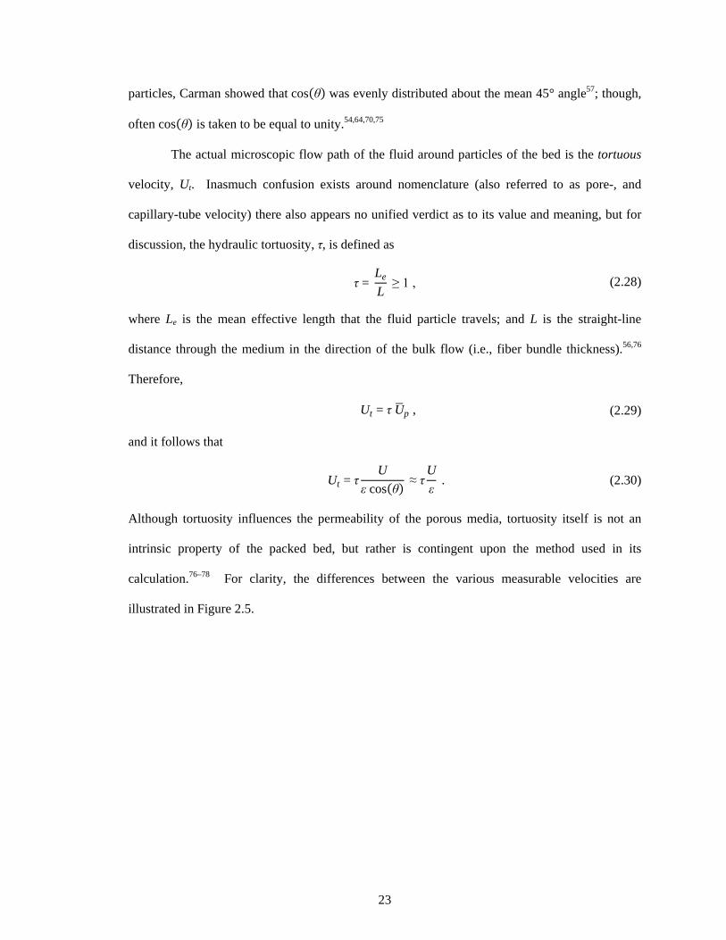
particles, Carman showed that cos(θ) was evenly distributed about the mean 45° angle57; though,
often cos(θ) is taken to be equal to unity.54,64,70,75
The actual microscopic flow path of the fluid around particles of the bed is the tortuous
velocity, Ut. Inasmuch confusion exists around nomenclature (also referred to as pore-, and
capillary-tube velocity) there also appears no unified verdict as to its value and meaning, but for
discussion, the hydraulic tortuosity, τ, is defined as
τ = Le
L ≥ 1 , (2.28)
where Le is the mean effective length that the fluid particle travels; and L is the straight-line
distance through the medium in the direction of the bulk flow (i.e., fiber bundle thickness).56,76
Therefore,
Ut = τ U�p , (2.29)
and it follows that
Ut = τU
ε cos(θ) ≈ τUε
. (2.30)
Although tortuosity influences the permeability of the porous media, tortuosity itself is not an
intrinsic property of the packed bed, but rather is contingent upon the method used in its
calculation.76–78 For clarity, the differences between the various measurable velocities are
illustrated in Figure 2.5.

24
Figure 2.5: Superficial, Physical, and Tortuous Velocity Superficial velocity, defined as the volumetric flow rate divided by the frontal surface area, is independent of porosity. Physical velocity accounts for the macroscopic flow through the porous media (a function of porosity) and may exist for 0< θ <180°, assuming no backflow. Tortuous velocity details the microscopic flow permeating around individual porous elements. The relationship between the three measures of velocity is: U ≤ U�p ≤ Ut.
2.4.8. Discussion
A porous medium can encompass a broad range of properties, composition, and
environmental conditions; all of which are parameters that influence the permeability of a fluid
(which itself may possess equal variety in nature). Because of the expansive variability in a
system involving a permeating fluid, the permeability of a porous material is largely domain-
specific. A brief survey of the literature will reveal numerous porous applications,
configurations, and measurements of permeability in addition to those presented here.79–85

25
Nevertheless, permeability is principally governed by a viscous and inertial resistance to fluid
flow, to the first- and second-order respectively. At low Re, permeability is linearly proportional
to the pressure drop and superficial fluid velocity; whereas at higher rates, the viscous resistance
becomes negligible and the inertial term dominates the pressure losses contributed by the fiber
bundle.
Often, the porosity of the volume and the empirical coefficients in Eq. (2.19) are used to
determine the permeability of the medium. Under this construct, porosity is an important
parameter since it appears as second- and third-power terms. Though it is more difficult to
ascertain in samples of unknown composition, porosity can easily be calculated from a device
with prescribed manufacturing specifications. However, although fractional void volumes might
be known, there may still exist uncertainties in the homogeneity, or isotropy of the packing
arrangement, where εeff ≠ ε. Therefore, for nontrivial cases, permeability is often verified using
additional forms of measurement.
2.5. Conventional Techniques for Visualizing Fluid Flow
Since the performance of a gas exchanger depends heavily on the fluid flow properties
through the fiber bundle, it is important to experimentally verify the permeability predictions of
the device and fiber membrane. Typically, optical methods provide real-time, non-invasive
measurements that are fairly simple in application, however, require specially designed housings
or specific materials. Quasi-optical imaging modalities such as magnetic resonance imaging
(MRI) and computed tomography (CT) can also provide relatively real-time acquisition and are
less restrictive to membrane materials, but often demand more complex principles and/or
reconstruction. Finally, several non-optical techniques offer good versatility, but usually
necessitate invasive or destructive methods to both the device and/or flow field.
26
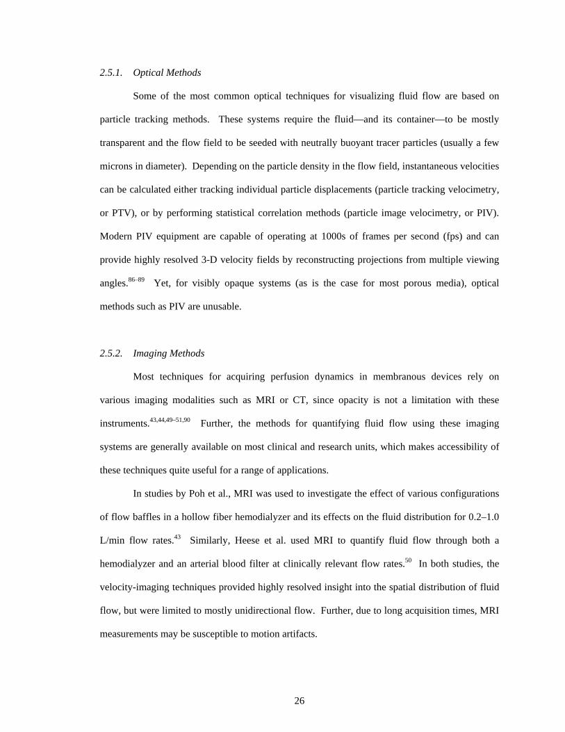
2.5.1. Optical Methods
Some of the most common optical techniques for visualizing fluid flow are based on
particle tracking methods. These systems require the fluid—and its container—to be mostly
transparent and the flow field to be seeded with neutrally buoyant tracer particles (usually a few
microns in diameter). Depending on the particle density in the flow field, instantaneous velocities
can be calculated either tracking individual particle displacements (particle tracking velocimetry,
or PTV), or by performing statistical correlation methods (particle image velocimetry, or PIV).
Modern PIV equipment are capable of operating at 1000s of frames per second (fps) and can
provide highly resolved 3-D velocity fields by reconstructing projections from multiple viewing
angles.86–89 Yet, for visibly opaque systems (as is the case for most porous media), optical
methods such as PIV are unusable.
2.5.2. Imaging Methods
Most techniques for acquiring perfusion dynamics in membranous devices rely on
various imaging modalities such as MRI or CT, since opacity is not a limitation with these
instruments.43,44,49–51,90 Further, the methods for quantifying fluid flow using these imaging
systems are generally available on most clinical and research units, which makes accessibility of
these techniques quite useful for a range of applications.
In studies by Poh et al., MRI was used to investigate the effect of various configurations
of flow baffles in a hollow fiber hemodialyzer and its effects on the fluid distribution for 0.2–1.0
L/min flow rates.43 Similarly, Heese et al. used MRI to quantify fluid flow through both a
hemodialyzer and an arterial blood filter at clinically relevant flow rates.50 In both studies, the
velocity-imaging techniques provided highly resolved insight into the spatial distribution of fluid
flow, but were limited to mostly unidirectional flow. Further, due to long acquisition times, MRI
measurements may be susceptible to motion artifacts.

27
Alternatively, Ronco et al. evaluated the uniformity and flow distribution in various
hollow fiber hemodialyzers manufactured with different fiber configurations using a clinical CT
scanner.44 Uniformity was assessed based on 1-D regional velocity calculations at defined
sections in a unidirectional flow field, and was useful for comparing velocities between flow in
the center of the device and that moving parallel along the peripheral walls of the unit. Likewise,
the study by Lu and Lu introduced an interesting method using CT imaging for tracking flow
through a densely bundled hollow fiber membrane, but their technique employed various
subjective thresholds and neglected to report additional analysis such as vector fields.51 Many
other applications, advantages, and limitations of measuring fluid flow with techniques based on
X-ray imaging will be discussed later in §2.6.
2.5.3. Non-Optical Techniques
Non-optical experimental techniques, such as those based on electrochemical and
convective methods have been used to evaluate membrane perfusion. In a study assessing the
uniformity of fluid flow for different membrane oxygenator designs, Hirano et al. placed 120
insulated copper electrodes throughout the fiber bundle and measured the time-dependent blood
perfusion by varying the electrical potential of the infused fluid at 1 and 5 L/min.52 Alternatively,
hot-wire anemometry (often, constant temperature anemometry, or CTA) has been used to
monitor local velocity changes by measuring convective losses from a thin wire.49 Both CTA and
electrochemical means provide real-time flow information, but each would require wires or
probes to be integrated into the membrane. In addition to imposing physical alterations which
could influence the normal flow properties, these methods provide limited spatial resolution and
only yield point-wise velocity information.

28
2.5.4. Discussion
Experimental evaluation of the perfusion dynamics though an opaque porous medium
such as a membrane oxygenator is a nontrivial problem. Optical methods for quantifying fluid
flow are ineffective in the absence of a transparent system, and non-optical methods generally
require invasive actions, are limited to single-dimensional measurements, and have poor spatial
resolution. Therefore, imaging modalities offer the most probable approach for obtaining
quantitative information of flow through a porous medium.
Phase contrast (PC) MRI can generate 3-D flow fields with excellent spatial resolution,
but require long acquisition times, which may be susceptible to fluctuations in the flow field.
Yet, recently, advances in FLASH MRI have generated 2-D image sequences with temporal
resolution of 20 ms and spatial resolution of 1.5–2 mm.91
Unfortunately, applications in MR imaging are limited by the physics of image
acquisition and reconstruction. For example, localized velocity averaging occurs for pixels
containing counter-current velocities or large discrepancies in nearby flow. Thus, in the case of
the hollow-fiber membrane oxygenator, pixels that overlap the fluid zone and the void regions in
neighboring fiber lumens would result in an underestimation of the local velocity. Further, the
presence of magnetic materials will disrupt the image signal.
Alternatively, CT imaging uses less complex image reconstruction methods than MRI,
requires lower acquisition times, and provides good spatial resolution. Despite the lower contrast
discrimination and spatial resolution than MRI, the faster temporal response means greater
invariance to motion artifacts, and for this reason, much has been done in developing methods for
measuring fluid flow using X-ray techniques.
2.6. X-ray Imaging for Measuring Fluid Flow
X-ray imaging modalities (including CT, angiography, etc.) offer high spatio-temporal
resolution which can be useful for real-time visualization of fluid flow. In medical applications,
29
rapid X-ray imaging techniques (up to 60 fps) are used for purposes of evaluating blood flow
perfusion through a vascular network, particularly in the treatment of cerebral aneurysms. 92–100
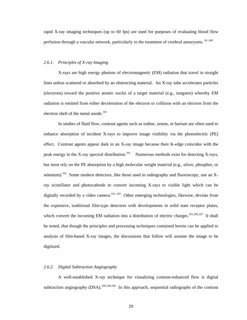
2.6.1. Principles of X-ray Imaging
X-rays are high energy photons of electromagnetic (EM) radiation that travel in straight
lines unless scattered or absorbed by an obstructing material. An X-ray tube accelerates particles
(electrons) toward the positive atomic nuclei of a target material (e.g., tungsten) whereby EM
radiation is emitted from either deceleration of the electron or collision with an electron from the
electron shell of the metal anode.101
In studies of fluid flow, contrast agents such as iodine, xenon, or barium are often used to
enhance absorption of incident X-rays to improve image visibility via the photoelectric (PE)
effect. Contrast agents appear dark in an X-ray image because their K-edge coincides with the
peak energy in the X-ray spectral distribution.101 Numerous methods exist for detecting X-rays,
but most rely on the PE absorption by a high molecular weight material (e.g., silver, phosphor, or
selenium).101 Some modern detectors, like those used in radiography and fluoroscopy, use an X-
ray scintillator and photocathode to convert incoming X-rays to visible light which can be
digitally recorded by a video camera.101–105 Other emerging technologies, likewise, deviate from
the expensive, traditional film-type detectors with developments in solid state receptor plates,
which convert the incoming EM radiation into a distribution of electric charges.101,106,107 It shall
be noted, that though the principles and processing techniques contained herein can be applied to
analysis of film-based X-ray images, the discussions that follow will assume the image to be
digitized.
2.6.2. Digital Subtraction Angiography
A well-established X-ray technique for visualizing contrast-enhanced flow is digital
subtraction angiography (DSA).100,108,109 In this approach, sequential radiographs of the contrast

30
perfusion are subtracted from a background (or “mask”) image taken prior to the infusion of the
dye.110,111 Once background details are removed, the image histogram is digitally enhanced to
optimize the image contrast visibility. This digital subtraction and enhancement technique
improves the signal-to-noise ratio (SNR) by eliminating background structures that would
otherwise convolute the flow features being imaged.
2.6.3. 2-D Videodensitometric Tracking Methods
In a series of X-ray images, the contrast density, D(x, y, z, t), of each pixel (2-D “picture
element”) is represented by a position in space at a given time. Since an X-ray image is a
measure of the penetrating EM radiation, D is already integrated over the z-direction (this is
discussed further in §2.6.4.). If the flow field can be assumed to be axisymmetric in the
orthogonal x and y planes (such as flow in a blood vessel or pipe), the contrast density can be
reduced to a single-dimension by integrating over the cross-section
D(x, t) = �D(x, y, t)dy , (2.31)
where {x, t} ≥ 0. 100
In general, bolus tracking algorithms for 2-D densitometric images fall in two categories:
time-density and distance-density methods. The former approach measures the transit time of the
contrast medium from one [defined] region to another; the latter calculates the distance traveled
between sequential frames (see Figure 2.6).92,94,100,109 Both time-density and distance-density
methods assume the contrast is evenly and homogenously distributed throughout the flow field;
an assumption that is usually satisfied if the contrast medium has a viscosity approximately equal
to the bulk fluid and has been infused at a rate greater-than or equal to the superficial velocity.94
Time-density tracking methods rely on observing changes in image intensity as a function
of time between two fixed regions of interest (ROIs). Numerous methods exist for measuring
bolus arrival times, including time-of: peak-to-peak; threshold density; center of gravity; leading

31
edge detection; etc.100 These algorithms have the advantage of being simple in construct, but are
ill-suited for analysis of instantaneous velocities in pulsatile flows.100
Distance-density methods, on the other hand, assess flow velocity by measuring the
distance a certain intensity threshold (e.g., 50% of maximum) travels between two successive
images. Distance-density methods are usually more accurate than time-density approaches since
spatial resolution is typically higher than temporal resolution.92 Yet, analysis based on a defined
threshold may be vulnerable to over-/under-estimation of the flow velocity, depending on how
changes in contrast intensity are defined.100
Figure 2.6: Time-Density and Distance-Density Bolus-Tracking Analysis Curves Time-density algorithms (left) measure the time difference between contrast-density curves for two defined ROIs; velocity is defined as the distance between the ROIs divided by Δt. Distance-density methods (right) calculate distance traveled between successive image frames according to a prescribed contrast threshold; velocity is defined as the distance between relative contrast levels divided by the time difference between successive images. The shape of the contrast density curves varies between inlet and outlet phases due to convective dispersion and/or branching of the infusion bolus.
2.6.4. Combining Multiple Imaging Projections
For a 3-D body, planar X-ray images provide little depth information since the X-ray
projection is a sum of the total attenuation effects between the source and detector. Visual clues

32
such as surface texture, shading, and occlusion are absent from image projections, and depth
perception is primarily achieved only from motion parallax in an image series.112,113 However,
the combination of two-or-more projections from different vantage points can be useful in
interpreting “z-plane” details through various reconstruction approaches.
The most common method of X-ray reconstruction—and the approach used by most CT
scanners—is performed through Fourier back-projection or similar algebraic techniques.101 Using
multiple projections spaced rotationally around an object, images are overlaid, or reconstructed,
into 3-D renderings, with better clarity achieved from a greater number of image projections (see
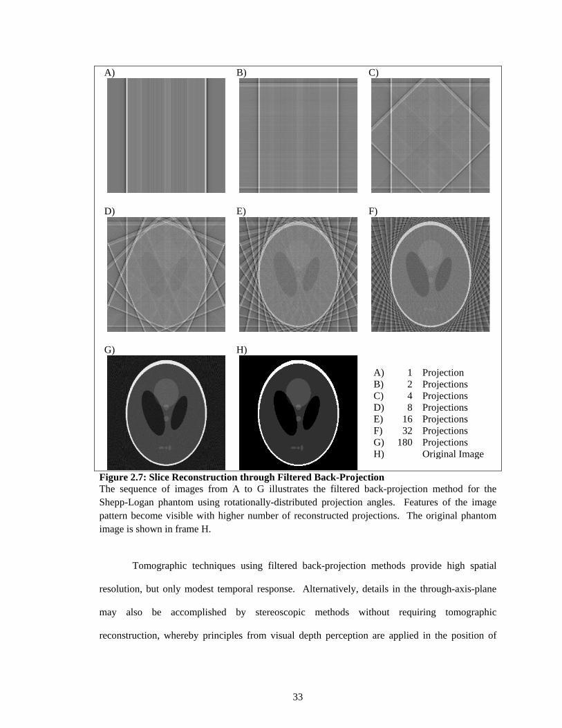
Figure 2.7).
33
A) B) C)
D) E) F)
G) H)
A) 1 Projection B) 2 Projections C) 4 Projections D) 8 Projections E) 16 Projections F) 32 Projections G) 180 Projections H) Original Image
Figure 2.7: Slice Reconstruction through Filtered Back-Projection The sequence of images from A to G illustrates the filtered back-projection method for the Shepp-Logan phantom using rotationally-distributed projection angles. Features of the image pattern become visible with higher number of reconstructed projections. The original phantom image is shown in frame H.
Tomographic techniques using filtered back-projection methods provide high spatial
resolution, but only modest temporal response. Alternatively, details in the through-axis-plane
may also be accomplished by stereoscopic methods without requiring tomographic
reconstruction, whereby principles from visual depth perception are applied in the position of

34
two-or-more X-ray sources with angles of separation ranging from a few degrees to fully
orthogonal.103,112–114 The offset between the two sources leads to slightly different images (viz.,
line integrals), and together generate a stereoscopic field of view (FOV), where corresponding
markers in the stereoscopic image pair can be extrapolated to identify their 3-D position (see
Figure 2.8).
Figure 2.8: Illustration of Stereoscopic Reconstruction Offsetting two-or-more X-ray sources/detectors about a central rotational axis provides alternative viewing angles useful for 3-D depth information. The area of overlap characterizes the stereoscopic FOV. Points existing in the FOV generate unique positions according to the combined locations between different image projections, and therefore allow spatial reconstruction in the stereoscopic z-plane. Depth resolution is dictated by the pixel spacing of image projections.

35
When unique features or markers in the stereoscopic projections are limited, or possibly
indistinguishable, various strategies have been developed—mostly based on iterative processes.
Since reconstruction from two planar images is an ill-formed problem, these techniques usually
require a priori information and/or restrictive assumptions. For example, when reconstructing
patient vasculature from biplane X-ray radiographs, Pellot et al. originally prescribed an elliptic
approximation for the vessels, and then used an optimization algorithm to recursively deformed
the shape according to back-projection gray-level (i.e., contrast density) values (Figure
2.9A).115,116 Similarly, Prause et al. used a 3-D anatomical model of the heart as the initial
framework for iterative reconstruction of the left and right ventricles imaged with biplane
angiography (Figure 2.9B).117
Figure 2.9: Iterative Reconstructive Methods from Biplane Angiography A) Iterative reconstruction of a branching vessel based on deforming 2-D elliptical approximations. Image courtesy of Pellot et al.116 B) Binary reconstruction of the left ventricle from biplane image projections. The average shape of 20+ patient hearts served as an initial template by which further iterations were guided. Image courtesy of Prause et al.117 Most reconstruction methods construct volumetric models from stacks of 2-D data.

36
2.6.5. Discussion
The high spatio-temporal resolution of X-ray imaging techniques has encouraged
numerous studies for measuring fluid flow in opaque systems that were previously inaccessible
with optical methods. X-ray velocimetry utilizes the same principles as optical PTV and PIV and
has been shown to be a reliable tool in both 2-D and 3-D applications.102–104,118 Further,
techniques such as X-ray DSA improve visualization of the contrast-enhanced flow and can be
performed real-time. Yet, selection of the appropriate X-ray imaging approach is study-specific.
CT lacks temporal response for dynamic events and requires advanced reconstruction algorithms
from multiple image projections, whereas non-tomographic means are generally simpler to
implement, interpret, and faster in acquisition, but often require incorporation of approximations
and assumptions. Features of the flow field such as pulsatility and the extent to which the flow is
axisymmetrical will also narrow applicable measurement strategies.
For instance, bolus-tracking methods are, computationally, relatively simple, but are ill-
suited for pulsatile flows and may result in incorrect measurements for non-plug flow, divergence
in the contrast bolus, or in the case of backflow.100 In addition to assuming a homogenous
contrast distribution, most 3-D (and some 2-D) reconstruction methods require a linear
relationship between changes in the X-ray intensity and density of the contrast agent.15,115,117,119
Three-dimensional reconstruction of fluid flow using limited (e.g., two) projections can
be useful in estimating the z-plane profile, but the problem remains ill-posed since two
projections are not sufficient to resolve all of the through-plane information—even in sparse
systems. Since X-ray projections represent sums of the total attenuation of the X-ray beam
through the absorptive medium, images lack depth clues such as reflection, occlusion, and surface
texture. Further, gray-level intensities, based on contrast density, might provide some depth
perception, but are uninformative at steady maximum opacity of the image field due to unknown
exact peak values.92 Often, strategies such as incorporating a priori information or reducing the
system to a binary flow field can improve reconstruction approximations, but are limited to
37
application-specific venues.114–117 Still, others have developed algorithms based on motion
parallax and convective dispersion models using rotational projections.99,120
Although numerous assumptions and approximations are often utilized to resolve
information from planar X-ray images, image projections do provide useful details regarding the
dynamic behavior of fluid flow in opaque systems. In applications of CFD verification and
validation, X-ray imaging techniques can be helpful for supporting numerical results, whereas the
CFD simulations can be used to resolve specific features in the flow field.
2.7. Conclusions
The development of a suitable gas exchange device for long-term respiratory support
requires evaluation of various factors and design configurations to improve the biocompatibility
and performance of the device. Numerical simulations are valuable in providing predictions of
physical data and can help lower the amount of experimental testing, but the accuracy of CFD
studies is ultimately limited by the strength of the underlying models and assumptions
incorporated into the governing equations of fluid flow. Validation of CFD results in membrane
oxygenators traditionally has been based on comparison of numerical and experimental pressure
distributions alone, since direct observation of the perfusion dynamics is difficult to accomplish
due to the opacity of the fiber bed. However, the availability of X-ray imaging modalities to
provide real-time, non-invasive assessments of fluid flow in opaque systems presents an
opportunity for validating numerical simulations of fluid flow in membrane oxygenators.
© Cameron C. Jones 2012

38
3. CFD MODEL 3.1. Overview of the Test Device
A schematic of the general flow direction in the Affinity Oxygenator (Affinity NT®
Oxygenator, Medtronic, Minneapolis, MN) is shown in Figure 3.1. Deoxygenated blood from the
patient enters the device and passes through a heat exchanger to maintain body temperatures
during device usage. The venous blood flows up the inlet tube, reverses direction in the inner
flow channels, and permeates through the fiber bundle in a radial fashion. Gas exchange occurs
in the fiber bundle region of the device due to local diffusion gradients, and is collected in an
outer gap before exiting the outlet port.

39
Figure 3.1: Representation of the Test Device The general flow path in the Affinity NT® Oxygenator: Deoxygenated blood enters from the bottom left of the device, passes over the heat exchanger, and continues upward through the inlet tube. After reaching the top of the device, blood changes direction and flows down tapering channels, which facilitate an even distribution across the inner diameter of the fiber bundle. Gas exchange occurs in the fiber bundle and blood is collected in an outer gap, upon which the oxygenated blood is returned to the patient.
3.2. Computational Domain
Geometrical representations of the membrane oxygenator were drawn in a commercial
CAD program (SolidWorks 2007, SolidWorks Corp., Concord, MA), and meshed (ANSYS®
Meshing 12.1, ANSYS Inc., Canonsburg, PA) prior to solving Eqs. (2.6) and (2.23) for the flow
field. Commercial CFD software (ANSYS® Fluent v12.1, ANSYS Inc.) was used to approximate
the equations of fluid motion in the absence of any turbulence model. The geometric model
consisted of three fluid regions: the inner flow (inlet tube and inner flow channels), an annular

40
fiber bundle, and the outer flow (an outer gap between the fiber bundle and housing and the outlet
port); the heater was not included in the computational domain (see Figure 3.2).
Figure 3.2: Computational Fluid Zones The figure illustrates the three fluid zones defined in the CFD model: inlet tube and inner flow channels; fiber bundle; outer flow gap and outlet port. Inlet and outlet faces were defined normal to the inlet tube and outlet port, respectively. The dotted surface represents the plane of symmetry, modeled using a slip condition.
3.3. Boundary Conditions and Model Assumptions
CFD simulations were conducted for flow rates in the range 1.0–4.5 L/min. A constant
inlet velocity (in m/s) was prescribed by dividing the volumetric flow rate by the inlet cross-
sectional area (defined normal to the boundary), and a zeroed reference pressure at the outlet. To
reduce computational expense, a symmetry (slip) condition was assigned to the problem domain
boundaries formed from bisecting the oxygenator along the device’s symmetric midline as
implied by Figure 3.2, and a no-slip condition was assigned to all solid surfaces (Figure 3.2).

41
Further, gravitational effects were not included in the computational model; hence FB ≡ 0 in Eq.
(2.23). Simulations were performed assuming standard operating pressure (101325 Pa).
Blood was modeled as a Newtonian fluid with constant viscosity (3.3 cP) and density
(1050 kg/m3) undergoing incompressible laminar flow. The fiber membrane was treated as a
lumped porous medium incorporated into the N.–S. equations as a single momentum sink
according to the Ergun equation (2.24); the viscous and inertial permeability coefficients were
defined using dp = do. Due to the high packing density of the woven fiber bundle (45%), the
permeability was assumed to be isotropic.39,40,42
Fluent was executed using second-order spatial derivation approximations except for
advective terms appearing in Eq. (2.23); these were treated with the usual first-order upwind
procedure. A convergence criterion of 10−4 for the continuity equation and velocity component
recoupling iterations was employed in achieving a steady flow solution. A summary of the
boundary conditions and model parameters are listed in Table 3.1.
Table 3.1: CFD Boundary Conditions and Model Parameters
Inlet Velocity 0.098–0.441 m/s Outlet Pressure 0 Pa Symmetrical Midline slip condition All Solid Surfaces u1 = u2 = u3 = 0 (no slip condition) Density, ρ 1050 kg/m3 Viscosity, μ 0.0033 kg/m s (3.3 cP) Outer Fiber Diameter, do 0.0003 m Porosity, ε 0.45 Permeability, k 1.8074E−10 m2 Darcy Coefficient, α 150 Inertial Loss Coefficient, β 3.5
Note: Inlet velocities are defined as the volumetric flow rate divided by the inlet cross-sectional area; the outlet pressure is relative to the inlet. Darcy and inertial loss coefficients are the conventional Ergun terms.54
42
3.4. Grid Function Convergence
The grids used in this investigation were generated using unstructured 3-D
tetrahedral/hybrid grid cells (see Figure 3.3). Convergence tests of the numerical solutions were
performed with six grid sizes ranging from 20K to 1.72M cells, using the grid with the highest
resolution as the theoretical exact solution, denoted f (cf. Eq. 2.8). The error between f and grid
functions from coarser grids, f*, was quantified using a Euclidean norm composed of the
dimensionless pressure drop, p*, and maximum velocity, u*, across the device; this norm was
defined as
‖e‖2 = �1𝑛�� fi − f i
*�2
n
i = 1
�
12
, (3.1)
where 𝒇∗ ≡ ( p*, u* )T; and n is number of grid cells. Pressure and velocity components were
made dimensionless by dividing by the dynamic pressure and inlet superficial velocity
magnitude, Uinlet, respectively as
p* = ∆p
12 ρUinlet
2 , (3.2)
and
u* = umax
Uinlet , (3.3)
where umax is the maximum velocity within the device.

43
Figure 3.3: CFD Mesh The conformal mesh contains 1.72M elements and employs a symmetry boundary condition along the device’s vertical midline. The grid color identifies the three fluid zones: inlet (green), fibers (gray), and outlet (blue).
The error norms were fitted using a least-squares correlation, which characterized the
convergence rate of the second-order numerical method as 1.69 (see Figure 3.4). The grid with
the highest resolution was selected for all data representation, where pressure drop and velocity

44
vectors for the finest mesh are estimated to be within an error band of 3.3% and 1.6% of the
continuum values, respectively. The numerical values used in the order of convergence
calculations are listed in Table 3.2. Although stronger measures of convergence could be
obtained from point-wise truncation error analysis, large disparities between velocities in the
porous media region of the device versus the non-porous regions (~102) would negate
contributions of the velocity convergence in Eq. (3.1).
Figure 3.4: Grid Function Convergence The order of convergence for the numerical studies is shown to be 1.69. Each of the coarser grid functions were subtracted from the finest mesh (theoretical solution) and their errors are plotted above. The pressure and velocity components of the mesh with the highest resolution were calculated to be within 3.3% and 1.6% of the continuum values, respectively.
Table 3.2: Grid Function Convergence Values
Elements (× 1000) Step Size, h Δp (kg/m s2) umax (m/s) p* u* error
norm 27 1.0 1649.5 0.967 3.363 4.933 0.582 47 0.8 1670.3 0.954 3.494 4.866 0.679 90 0.6 1691.7 1.030 3.032 5.256 0.258
272 0.4 1749.9 1.050 3.022 5.355 0.198 597 0.3 1761.6 1.074 2.908 5.479 0.079
1720 0.2 1768.7 1.090 2.832 5.562 N/A
© Cameron C. Jones 2012

45
4. BIPLANE DSA 4.1. Experimental Setup
An important value to X-ray imaging analysis is that no modifications are required for the
device in order to allow application of the technique (i.e., a “non-destructive” method). Since
most constituents of commercial membrane artificial lungs are polymer-based materials, X-rays
can easily penetrate the device, providing a peek at the internal flow properties. In biplane
angiography, synchronous X-ray sources and detectors are positioned in orthogonal planes to
provide real-time 2-D flow information. Further, the excellent spatio-temporal resolution of DSA
is readily available in most clinical angiography suites. These features therefore enable insight
into characteristics of the fluid flow through the membrane oxygenator that can be compared
directly with CFD predictions.
4.1.1. Configuration of the X-ray System
A conventional clinical X-ray system was used for acquiring experimental perfusion data
due to its availability, high temporal resolution, and relatively inexpensive application. Biplane
DSA images were acquired by a Siemens Artis zee Biplane system (Siemens, Malvern, PA) at 7.5
fps for a contrast-enhanced flow through the Affinity membrane oxygenator. The oxygenator
was oriented such that orthogonal X-ray acquisitions bisected the inlet flow channel in order to
provide information regarding symmetry of the flow through the fiber membrane (see Figure
4.10).

46
Figure 4.10: Experimental Setup of Biplane Projections Orthogonal biplane X-ray sources were configured to obtain image projections along the inlet tube at 7.5 fps.
4.1.2. Configuration of the Fluid Circuit
The bench circuit consisted of a 37% by weight aqueous-glycerin solution at 21°C
(comparable to normal patient blood viscosity) and was circulated with a centrifugal pump
(CentriMag®, Levitronix®, Zurich, Switzerland) at flow rates ranging 1.0–4.5 L/min as measured
by a Transonic Systems bypass flow meter (HT110, Transonic Systems Inc., Ithaca, NY). One
hundred fifty milliliters of an iodinated contrast agent iohexol (Omnipaque™ 300 mgI/mL, GE
Healthcare Inc., Waukesha, WI), diluted to a room temperature viscosity of 3.3 cP, was infused
through an inline port 1 m upstream of the oxygenator inlet at the same flow rate as the bench

47
circuit. Biplane images were acquired for 20 s to allow full visualization of the dye entering and
leaving the device. A summary of the study parameters are in Table 4.1.
Table 4.1: Experiment Study Parameters
Flow Rate, Q 1.0–4.5 L/min Blood Analogue 37% w/v aqueous-glycerin solution Ambient Temperature 21°C Contrast Volume 150 mL
4.2. Analysis of Angiographic Images
All image analysis and post-processing was performed in MATLAB® (v.7.12 R2011a,
The MathWorks, Inc., Natick, MA) using a custom code (pseudo-language algorithms are
provided in Appendix C).
4.2.1. Image Processing
The study-generated DICOM image files were imported into MATLAB and the
maximum background intensity (threshold) was subtracted from all subsequent images. All pixel
values above the threshold were assigned a value of 1; those below, a value of 0. The binary
images were then digitally rotated and cropped for proper spatial alignment with the
complementary biplane projection using known markers on the oxygenator housing. The spatial
and temporal resolution was known to be 0.2 mm and 0.133 s, respectively.
Prior to analyzing the flow field data, a median filter121 using the nearest 3 × 3
neighboring points was used to reduce noise and preserve edges of the digital images for
improved handling of the velocity estimates.122 In 2-D form, the median filter consists of an M ×
M window (M must be odd), where the median of the discrete sequence of elements replaces the
middle value of the window. Following spatial smoothing by the median filter, a flood-fill

48
operation was used to fill remaining “holes” in the contrast image. These functions are illustrated
in Figure 4.2.
Figure 4.2: Image Processing Operations Prior to flow-field measurements, the image dataset undergoes several iterations of image smoothing. Rough pixilations are smoothed with a median filter using a 3 × 3 pixel window, and a flood-fill operation is used to fill holes in the contrast medium. Representative regions have been highlighted for clarity.
4.2.2. Maximum Cross Correlation Method
Propagation of the contrast wave through the membrane was tracked using a maximum
cross correlation (MCC) method, which identifies pattern-based correlations between two
sequential time-dependent images. Though the MCC method is a non-traditional application of
X-ray image analysis, the method has been shown to be a reliable tool for assessing progression
of flow.123–125 In this approach, a grid is mapped over the image at a time step, ti, dividing the

49
image projection into a series of templates. For each template, a larger grid (referred to as the
search window) is mapped in the subsequent X-ray image, ti+1; whereby the corresponding search
window in ti+1 is large enough to encompass the maximum distance the flow might progress
between sequential image frames (see Figure 4.3). In a 2-D projection, each element in the
resulting matrix contains a correlation value from −1.0 to 1.0 based on the degree of similarity
between the image and the template features. The normalized correlation coefficient matrix, C, is
obtained by
C(v, w)= ∑ ��I(x, y) − Iv̅, w�[T(x − v, y − w) − T�]�x, y
�∑ �I(x, y) − Iv̅, w�2
x, y ∑ [T(x − v, y − w) − T�]2x, y
, (4.1)
where the pixel values of the search window are I(x, y); Iv̅, w is the average value of I(x, y) in the
region under the template, T, positioned at v, w; and T� is the average template value.126 The
maximum value of the cross correlation matrix indicates the most probable likelihood of the
template’s displacement, while the vector at each grid point is given by
c = �(v)2+(w)2
∆t , (4.2)
and
θ = arctan �wv� , (4.3)
where c is the velocity magnitude (in pixels/s); t is the time between sequential images (1/fps);
and θ is the vector orientation.

50
A) B)
C) D)
Figure 4.3: Maximum Cross Correlation Function The MCC method identifies the most likely displacement between two successive ROIs according to the correlation of pattern-based geometries. A) The red box indicates the template at time ti, centered at a specific grid point. B) The flow field is advancing from left-to-right at position ti+1; the template from the previous time step is shown for reference and the entire field-of-view characterizes the search window. C) A correlation map portrays the correlation of the template (red box of ti) with the new flow field in ti+1. D) The vector according to the maximum correlation is drawn for the given grid point.

51
4.2.3. MCC Filtering Algorithms
The MCC method requires the user to define both template and search window sizes,
with the only two conditions being: the search window encompasses the maximum distance the
template would travel in a given time-step; and the template contains enough features to be
distinguishable. Therefore, it is no surprise that the values one chooses for template and search
window boundaries can influence the final output. Moreover, it is entirely likely that false
positive correlations may exist, whereby the template corresponds better with a random structure
of the flow field than with the true fluid movement.
To reduce the subjectivity in defining template and search window sizes, iterations were
run using rectangular template sizes ranging from 5 to 53 pixels per side (pps), and search
window sizes ranging from 13 to 149 pps (recall, digital resolution is 5.333 pixels/mm). For each
template size, the average velocity in the fiber bundle calculated by each search window was
averaged and is graphed in Figure 4.4, where the error bars indicate standard deviation between
the averages computed by the different search windows. As might be expected from a pattern-
based correlation method, larger templates will be more robust against false positives. Indeed, as
represented in Figure 4.4, increasing the template size led to more constant and consistent
correlations. The maximum template (53 pps) and search window (149 pps) sizes were used for
the analysis in this study.
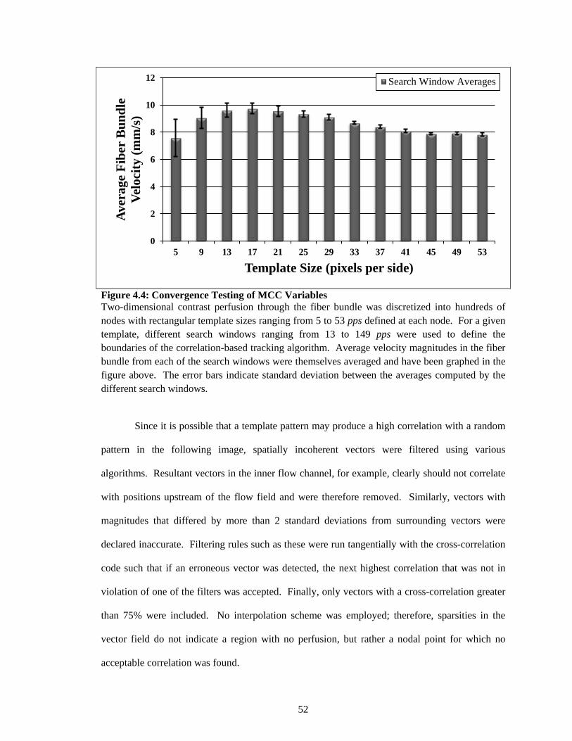
52
Figure 4.4: Convergence Testing of MCC Variables Two-dimensional contrast perfusion through the fiber bundle was discretized into hundreds of nodes with rectangular template sizes ranging from 5 to 53 pps defined at each node. For a given template, different search windows ranging from 13 to 149 pps were used to define the boundaries of the correlation-based tracking algorithm. Average velocity magnitudes in the fiber bundle from each of the search windows were themselves averaged and have been graphed in the figure above. The error bars indicate standard deviation between the averages computed by the different search windows.
Since it is possible that a template pattern may produce a high correlation with a random
pattern in the following image, spatially incoherent vectors were filtered using various
algorithms. Resultant vectors in the inner flow channel, for example, clearly should not correlate
with positions upstream of the flow field and were therefore removed. Similarly, vectors with
magnitudes that differed by more than 2 standard deviations from surrounding vectors were
declared inaccurate. Filtering rules such as these were run tangentially with the cross-correlation
code such that if an erroneous vector was detected, the next highest correlation that was not in
violation of one of the filters was accepted. Finally, only vectors with a cross-correlation greater
than 75% were included. No interpolation scheme was employed; therefore, sparsities in the
vector field do not indicate a region with no perfusion, but rather a nodal point for which no
acceptable correlation was found.
0
2
4
6
8
10
12
5 9 13 17 21 25 29 33 37 41 45 49 53
Aver
age
Fibe
r B
undl
e Ve
loci
ty (m
m/s
)
Template Size (pixels per side)
Search Window Averages
53
4.2.4. Point Cloud Reconstruction
The orthogonal biplane projections provide only limited insight into the 3-D flow
properties (cf. §2.6.4.), but with reasonable assumptions, useful qualitative information may be
obtained. For each time step, the cumulative perfusion for both image projections was outlined
by a 2-D boundary, which traced the outer edge of the fluid perfusion and the internal features of
the oxygenator housing. The boundaries were divided into horizontal slices with a thickness of 1
pixel. Pixels for each of the biplane projections served as the nodal points in a cubic spline
interpolation—existing in the horizontal, or z-direction (see Figure 4.5). The interpolant was
constructed with a high resolution of points to help improve smoothing and reconstruction.
For each point in the interpolant, its 3-D spatial position and normal component were
stored in an N × 6 matrix, where N indicates the number of slices in a given time step. Since the
dye is assumed to be homogenously dispersed in the bulk fluid, and earlier imaging processing
steps eliminated “holes” in the binary perfusion image, the maximum number of ‘ON’ pixels for
each horizontal slice ranged from 1 to 6. The resulting point cloud was exported to MeshLab
(v.1.3.0, Visual Computing Lab, ISTI-CNR) which overlaid surfaces on the 3-D point set.

54
A)
B)
Figure 4.5: Biplane Image Interpolation Technique A) The interpolation algorithm required exactly 2 or 6 matching points between the two biplane projections for reconstruction of the interpolant. B) Corresponding points from each horizontal row were used as vertices for the cubic spline interpolation existing in the z-plane.

55
4.2.5. Image Processing Assumptions
As with all methods of contrast-enhanced flow, the contrast agent has been assumed to be
homogenously dispersed throughout the transport fluid. By ensuring the dye has approximately
the same viscosity as the fluid medium and infusion rates match the superficial bulk velocity, this
condition is usually satisfied.
In both MCC and point-cloud reconstruction studies, the most significant requirement
was to assume that the leading (or outer) edge of the dye was in the projected image plane. Since
densitometric images are integral projections, no information exists for through-plane velocities.
However, based on the annular structure of the Affinity Oxygenator and the woven fiber bundle,
the shortest flow path, when observing the device’s cross-section, would be direct lateral
perfusion (i.e., radial perfusion). This was confirmed by comparing the orthogonal biplane
projections, which showed nearly identical densitometric profiles (discussed further in §5.2.3.).
Furthermore, since the assumption of visually 2-D flow provided no details of through-plane flow
movement, the binary images were defined to be in the bisecting image plane.
© Cameron C. Jones 2012
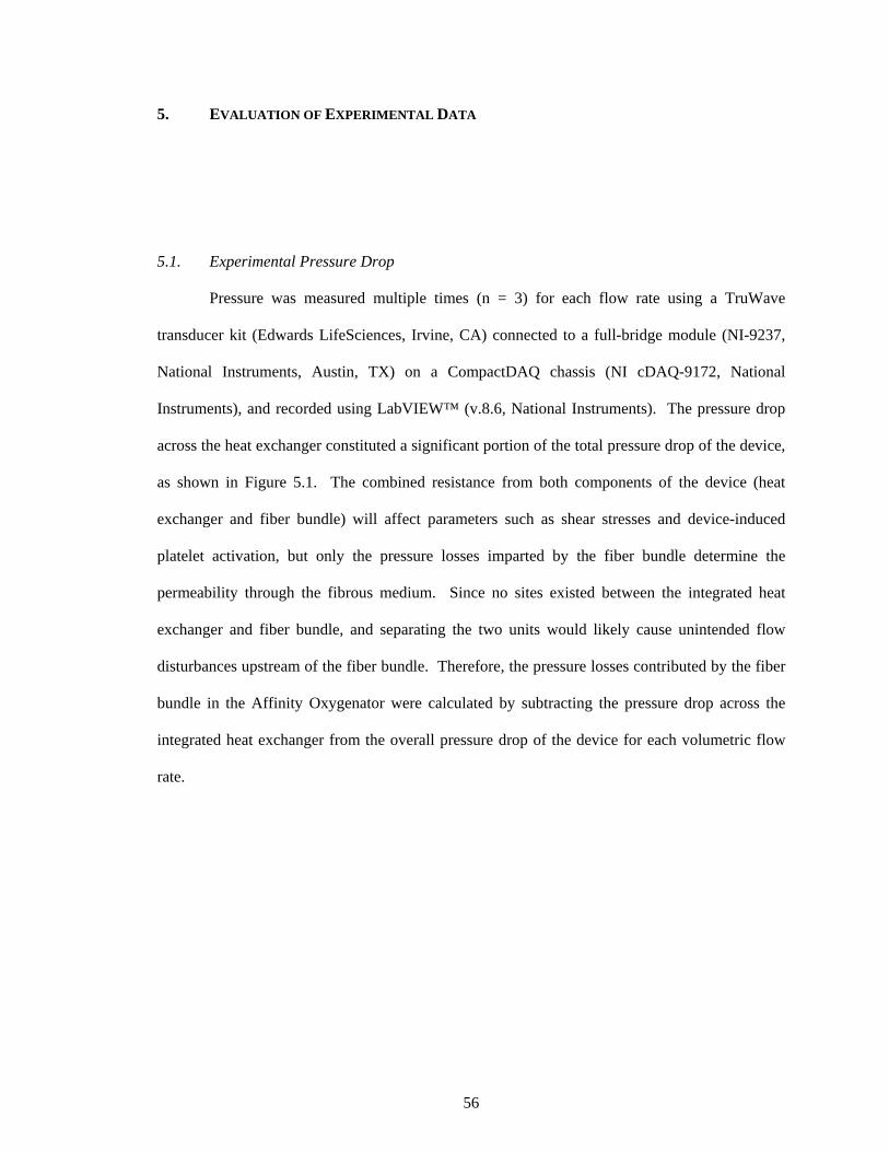
56
5. EVALUATION OF EXPERIMENTAL DATA 5.1. Experimental Pressure Drop
Pressure was measured multiple times (n = 3) for each flow rate using a TruWave
transducer kit (Edwards LifeSciences, Irvine, CA) connected to a full-bridge module (NI-9237,
National Instruments, Austin, TX) on a CompactDAQ chassis (NI cDAQ-9172, National
Instruments), and recorded using LabVIEW™ (v.8.6, National Instruments). The pressure drop
across the heat exchanger constituted a significant portion of the total pressure drop of the device,
as shown in Figure 5.1. The combined resistance from both components of the device (heat
exchanger and fiber bundle) will affect parameters such as shear stresses and device-induced
platelet activation, but only the pressure losses imparted by the fiber bundle determine the
permeability through the fibrous medium. Since no sites existed between the integrated heat
exchanger and fiber bundle, and separating the two units would likely cause unintended flow
disturbances upstream of the fiber bundle. Therefore, the pressure losses contributed by the fiber
bundle in the Affinity Oxygenator were calculated by subtracting the pressure drop across the
integrated heat exchanger from the overall pressure drop of the device for each volumetric flow
rate.
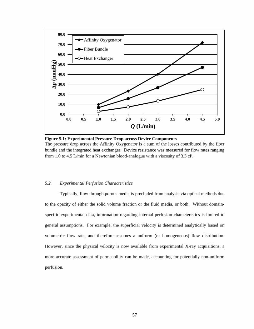
57
Figure 5.1: Experimental Pressure Drop across Device Components The pressure drop across the Affinity Oxygenator is a sum of the losses contributed by the fiber bundle and the integrated heat exchanger. Device resistance was measured for flow rates ranging from 1.0 to 4.5 L/min for a Newtonian blood-analogue with a viscosity of 3.3 cP.
5.2. Experimental Perfusion Characteristics
Typically, flow through porous media is precluded from analysis via optical methods due
to the opacity of either the solid volume fraction or the fluid media, or both. Without domain-
specific experimental data, information regarding internal perfusion characteristics is limited to
general assumptions. For example, the superficial velocity is determined analytically based on
volumetric flow rate, and therefore assumes a uniform (or homogeneous) flow distribution.
However, since the physical velocity is now available from experimental X-ray acquisitions, a
more accurate assessment of permeability can be made, accounting for potentially non-uniform
perfusion.
0.0
10.0
20.0
30.0
40.0
50.0
60.0
70.0
80.0
0.0 0.5 1.0 1.5 2.0 2.5 3.0 3.5 4.0 4.5 5.0
Δp (m
mH
g)
Q (L/min)
Affinity Oxygenator
Fiber Bundle
Heat Exchanger
58
5.2.1. Modified Residence Time
Most studies that investigate fluid flow through fibrous media derive permeability
equations based on the assumption that all fibers are aligned (oriented either parallel or
perpendicular to the flow direction) and experience a uniform flow field.60 Following this
condition of a uniform, radial flow through the fiber bundle, the average fluid residence time, tR,
is simply
tR = ∆xU�p
, (5.1)
where Δx is the fiber bundle thickness; and U�p is the average physical velocity. Yet, if the flow is
not entirely radial in propagation, U�p cannot be assumed to be equal to its analytical value (Eq.
2.27), and therefore tR remains unknown.
To account for potentially non-uniform perfusion, a modified residence time, tR', based
on peak-to-peak transit time,100 is expressed as
tR' = TN − TI , (5.2)
where TN is defined as the moment of peak intensity along the outer edge of the fiber bundle; and
TI is the time of peak intensity when contrast first enters the fiber bundle (Figure 5.2).

59
Figure 5.2: Modified Residence Time according to Time-Density Analysis The normalized contrast intensity curves characterize the time delay between ROIs defined at the inner and outer surfaces of the annular fiber bundle. Curves from the 2 L/min (dashed line) and 4.5 L/min (solid line) flow studies are represented above. Higher volumetric flow rates led to a faster up-stroke, less convective dispersion, and shorter residence time. Image acquisition was 7.5 fps.
The description of tR' in Eq. (5.2) is effectively a time-density calculation for two ROIs
defined at the inner and outer edges of the fiber bundle (cf. §2.6.3.). For the analytical
measurements, tR is significantly longer than the observed experimental data, which necessitated
the definition of tR' in Eq. (5.2). This is exemplified in Table 5.1.
Table 5.1: Calculated Residence Times
Q (L/min) tR (s) tR' (s) 1.0 8.65 6.53 2.0 4.32 2.73 3.0 2.88 1.87 4.5 1.92 1.27

60
5.2.2. Experimental and Analytical Fiber Bundle Velocities
Given tR', the experimental superficial velocity, U', was calculated by
U' = εU�p' = ε∆xtR'
, (5.3)
where U�p' is the average physical velocity calculated from the time-density analysis. The
differences between the analytical (Eq. 2.15) and experimental (Eq. 5.3) evaluations of U are
shown in Table 5.2. As would be expected, both U and U′ are linearly proportional to the
volumetric flow rate.
Table 5.2: Analytical and Experimental Superficial Velocities
Q (L/min) U (mm/s) U′ (mm/s) 1.0 1.16 1.53 2.0 2.31 3.66 3.0 3.47 5.35 4.5 5.20 7.90
5.2.3. Assessment of Perfusion Direction
The progression of the contrast-enhanced flow through the device at 2 L/min is shown in
Figure 5.3. Once the DICOM images had been converted to binary images and spatially
smoothed, the cumulative perfusion from previous images was subtracted from each new image,
revealing only the net new flow for the given time step (i.e., the current location of the advancing
contrast bolus). Flow travels up the inlet tube (Frames 1–3), into the tapering channels (Frame 5),
through the fiber bundle (Frames 5–23), into the outer gap (Frame 19), and exits through the
outlet port (bottom left of image, Frames 21–23).

61
Figure 5.3: Progression of Contrast Perfusion through the Fiber Bundle The image sequence shows the perfusion of the contrast bolus through the device at 2 L/min flow rate. The device inlet is located at the bottom center of the image frame (see Figure 3.2), and the outlet is positioned at the bottom left. Images were acquired at 7.5 fps. For clarity, every second image in the dataset was omitted in the display above.
Design of the flow channels along with packing density of the fibrous media contributes
to the mostly radial perfusion dynamics of the fluid flow. For all of the flow rates tested, no
preferential flow was observed due to the position of the outlet port. However, the progression of
the contrast wave front is not fully uniform, as is characterized by the uneven distribution of the
waveform in the vertical direction. This image series indicates that flow reaches the corners of
the device less readily (see specifically Frames 17–23), including the corner closest to the outlet
of the device. For the 2 L/min flow rate, most of the flow traveled through the bundle in
approximately 2.5 s (Frames 5–23)—visually reflective of tR' calculated in §5.2.1.
62
The construction of tR' is based on a 1-D calculation which has the benefit of allowing the
measurement to be partially invariant to non-uniform perfusion contours. In the annular fiber
bundle of the Affinity Oxygenator, if flow was indeed single-dimensional (viz., purely radial
flow) the average distance traveled by the contrast bolus in each image frame could be used to
calculate U�p', as opposed to the time-density techniques employed in Eq. (5.1). Therefore, it
might be logical to infer that deviations between the two measurements could yield information
regarding the degree of radial perfusion.
Calculations of the average contrast perfusion advancing through the fiber membrane
began once all of the dye had cleared the inner flow channels and was entirely contained in the
fiber bed. For each orthogonal projection, the left and right-side contrast waveforms were treated
as separate measurements. The pixel sum of the contrast in each segment was divided by the
vertical height of the fiber bundle to give the average thickness of the waveform if it were
compressed to a uniform surface. The physical velocity using the uniform perfusion method
�U�p''� was averaged for the duration where all of the flow existed in the fiber bundle. Once the
perfusion edge reached the outer gap, the measurement was terminated. The averages and
standard deviations of the waveforms for each of the flow rates are shown in Table 5.3. In all
cases, U�p'' was higher than U�p' which would suggest a perfusion waveform that is advancing with
deflections from purely radial flow. The percent of the flow that moves in a radial fashion is
obtained from the ratio between the two measurements.
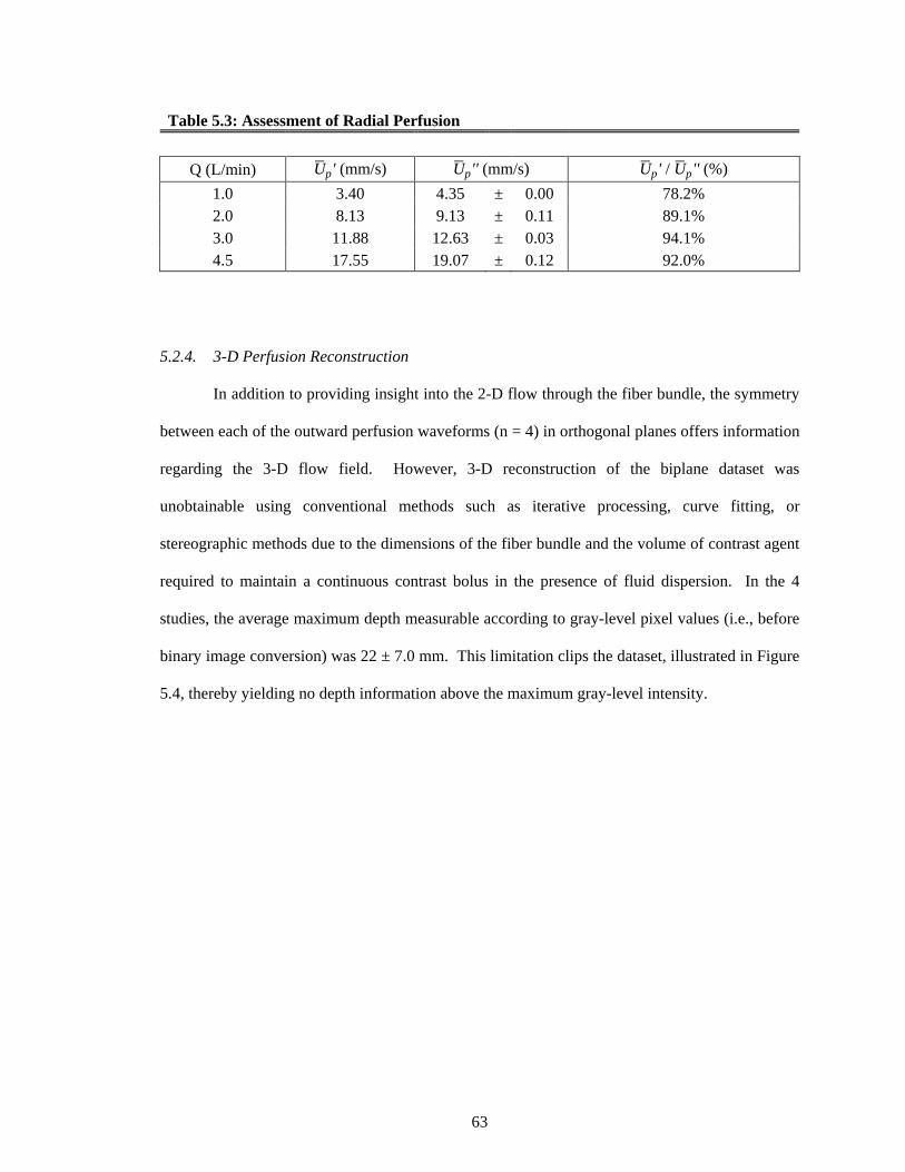
63
Table 5.3: Assessment of Radial Perfusion
Q (L/min) U�p' (mm/s) U�p'' (mm/s) U�p' / U�p'' (%) 1.0 3.40 4.35 ± 0.00 78.2% 2.0 8.13 9.13 ± 0.11 89.1% 3.0 11.88 12.63 ± 0.03 94.1% 4.5 17.55 19.07 ± 0.12 92.0%
5.2.4. 3-D Perfusion Reconstruction
In addition to providing insight into the 2-D flow through the fiber bundle, the symmetry
between each of the outward perfusion waveforms (n = 4) in orthogonal planes offers information
regarding the 3-D flow field. However, 3-D reconstruction of the biplane dataset was
unobtainable using conventional methods such as iterative processing, curve fitting, or
stereographic methods due to the dimensions of the fiber bundle and the volume of contrast agent
required to maintain a continuous contrast bolus in the presence of fluid dispersion. In the 4
studies, the average maximum depth measurable according to gray-level pixel values (i.e., before
binary image conversion) was 22 ± 7.0 mm. This limitation clips the dataset, illustrated in Figure
5.4, thereby yielding no depth information above the maximum gray-level intensity.

64
Figure 5.4: Data-Clipping resulting from Maximum Contrast Intensity Line profiles taken across the inlet tube (z = 15) and through the fiber bundle (z = 415) illustrate the limitation arising from a maximum contrast intensity. For the z-plane across the inlet tube diameter (15 mm) the cumulative contrast projection is fully characterized by the elliptical intensity curve. Alternatively, the z-plane through the base of the oxygenator housing (diameter is 82 mm) the maximum opacity of the contrast precludes any depth information. In the figure above, the contrast line integrals are displayed at 0.93-s intervals.
The qualitative symmetry observed between the biplane projections justified the
approximation of a radial perfusion contour. The outer edge of the contrast bolus in each aligned
biplane projection was assumed to be smoothly distributed in the non-orthogonal, z-plane
dimension, and the known 3-D position of the device housing was subtracted from the contrast
perfusion. Thus, for each row in the aligned projections, the algorithm required exactly two or
six reference nodes (see Figure 4.5). Due to the number of assumptions embedded in this
formulation, the 3-D volumetric perfusion remains only qualitative. Nevertheless, since the

65
algorithm interpolates in the non-orthogonal depth of field, the 3-D visualization maintains the
same level of quantitative accuracy as the 2-D biplane images, but provides improved spatial
clarity to the overall perfusion dynamics (see Figure 5.5).
Figure 5.5: Three-Dimensional Volumetric Perfusion at 2 L/min The outer edge of the biplane projections served as a set of vertices for the generation of a cubic spline in the z-direction. Each spline corresponded to a different slice in the z-plane, whose interpolated values were used to construct a point cloud in 3D. Surfaces were rendered over the point set to give clarity to the volumetric perfusion.
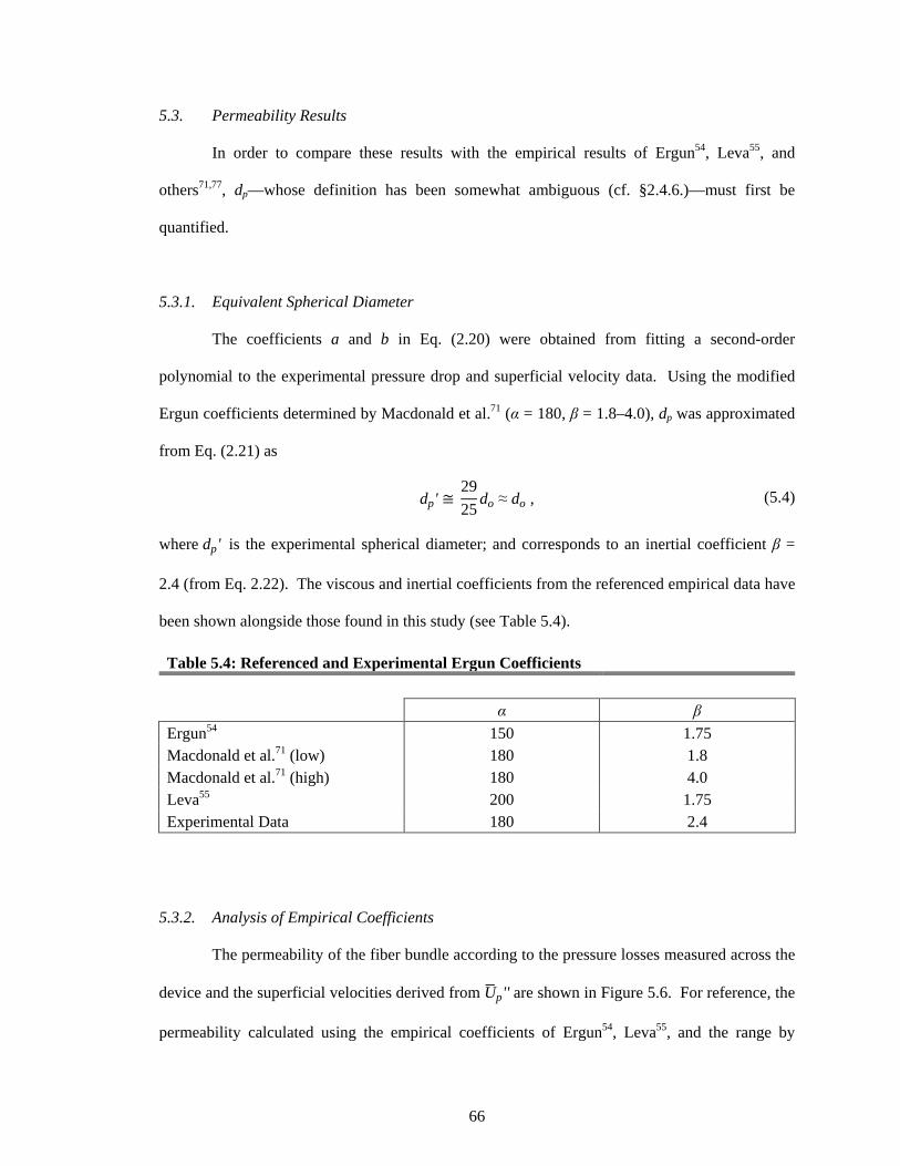
66
5.3. Permeability Results
In order to compare these results with the empirical results of Ergun54, Leva55, and
others71,77, dp—whose definition has been somewhat ambiguous (cf. §2.4.6.)—must first be
quantified.
5.3.1. Equivalent Spherical Diameter
The coefficients a and b in Eq. (2.20) were obtained from fitting a second-order
polynomial to the experimental pressure drop and superficial velocity data. Using the modified
Ergun coefficients determined by Macdonald et al.71 (α = 180, β = 1.8–4.0), dp was approximated
from Eq. (2.21) as
dp' ≅ 2925
do ≈ do , (5.4)
where dp' is the experimental spherical diameter; and corresponds to an inertial coefficient β =
2.4 (from Eq. 2.22). The viscous and inertial coefficients from the referenced empirical data have
been shown alongside those found in this study (see Table 5.4).
Table 5.4: Referenced and Experimental Ergun Coefficients
α β
Ergun54 150 1.75 Macdonald et al.71 (low) 180 1.8 Macdonald et al.71 (high) 180 4.0 Leva55 200 1.75 Experimental Data 180 2.4
5.3.2. Analysis of Empirical Coefficients
The permeability of the fiber bundle according to the pressure losses measured across the
device and the superficial velocities derived from U�p'' are shown in Figure 5.6. For reference, the
permeability calculated using the empirical coefficients of Ergun54, Leva55, and the range by

67
Macdonald et al.71 have also been graphed. The measured permeability of the device corresponds
well with the data of Leva and the lower permeability range determined by Macdonald et al.,
though the experimental data showed lower permeability and greater inertial resistance than those
of the conventional Ergun coefficients. Nevertheless, experimental permeability measurements
were relatively consistent with the empirical data, which would be expected based on the
agreements typically seen in CFD simulations.29,30,37–42
Figure 5.6: Fiber Bundle Permeability Pressure losses calculated using the empirical Ergun coefficients of Macdonald et al.71, Leva55, and Ergun54 have been plotted alongside the experimental pressure measurements (dashed line) according to the experimental superficial velocity.
5.4. Discussion
Validation of the numerical flow simulations require assessments of the fiber bundle
permeability to be accurately characterized. Early empirical studies laid the foundation for
today’s understanding of the viscous and inertial forces influencing flow through porous media.
0
1000
2000
3000
4000
5000
6000
7000
8000
9000
10000
0.000 0.001 0.002 0.003 0.004 0.005 0.006 0.007 0.008 0.009 0.010
Δp (k
g/m
s2 )
U (m/s)
ExperimentalErgunMacdonald (Low)Macdonald (High)Leva

68
For slow flows, the Darcy permeability describes resistance (i.e., pressure losses) to flow in a
linear relationship to the superficial velocity. As the velocity increases, momentum carries fluid
particles away from their streamlines and the inertial effects result in an increased flow resistance.
Conventionally, permeability is characterized by the pressure losses corresponding to the
superficial velocity. Yet, the superficial velocity does not explicitly describe the features of the
porous medium, including the porosity and packing arrangement. In fact, U is prescribed with
ε ≡ 0, therefore U portrays the volumetric flow rate as a uniform velocity field through the device.
When the porosity of the fluid zone is either randomly or isotropically distributed, and if the
container is large enough such that wall effects are negligible, a uniform superficial velocity is
generally an acceptable assumption. Yet, when perfusion is non-uniform or εeff ≠ ε , other
measures are required.
For the investigation above, the motivation for defining U based on tR' was due to the
observed non-uniformity of the velocity wavefront in the imaging acquisitions. Since the
angiographic images had been reduced to a binary flow field, the single-dimensional
approximation of the time-density method was valid for ROIs defined at the entry and exit
regions of the fiber bundle (cf. §2.6.3.). The only requirement of tR' is that the fluid perfusion is
rotationally symmetric; this was verified according to the similarities of the fluid propagation in
the orthogonal projections (Table 5.3).
In order to determine the degree of radial perfusion throughout the fiber bundle, a ratio
was established between the experimentally-derived physical fluid velocity and the average
thickness of the contrast bolus per time step. The method showed that as the flow rate increased,
the experimental velocity approached the velocity of the net new contrast in each image frame.
This may suggest that at higher flow rates (e.g., Q ≥ 2.0 L/min), the velocity direction through the
fiber bundle in the Affinity Oxygenator travels predominantly in a radial fashion.
© Cameron C. Jones 2012
69
6. EVALUATION OF NUMERICAL DATA 6.1. Flow Characteristics
The results from the CFD simulations correlated very well with the numerical data
obtained by Zhang et al. for a 5 L/min inlet flow rate through the Affinity Oxygenator.40 The
pressure distribution and flow characteristics from the numerical predictions were proportionally
consistent for all inlet velocities tested. In the following sections, all visualizations will be
represented by a clinically relevant 2 L/min flow rate. Perfusion through the device is depicted
by the pathlines illustrated in Figure 6.1. Blood flows up the inlet tube and reverses direction in
the inner flow channels. The tapered channels provide no resistance to the flow, which allows the
blood flow to fill the entire inner radius of the fiber bundle. The pathlines generated in the CFD
simulations show that the flow through the fiber bundle is mostly radial, and the position of the
outlet port does not appear to influence the perfusion of the flow more favorably towards the
device outlet. This was consistent with the DSA perfusion profiles, whereby the orientation of
the outlet port did not affect the uniformity of the radial distribution for any of the flow rates
ranging 1–4.5 L/min.

70
Figure 6.1: CFD Pathlines of Fluid Flow Three-dimensional pathlines through the fiber bundle are shown according to velocity magnitude (at 2 L/min). The pathlines illustrate flow through the inlet tube (bottom-middle of figure), reversal of direction in the inner channels, and radial perfusion through the fiber bundle. Once flow reaches the outer gap it circulates towards the device outlet (bottom-left).
Once the blood flow has permeated through the fiber bundle, it is collected in an outer
gap (3 mm thickness) and circulates to the outlet port. Upon exiting the device, the flow speed is
accelerated, as depicted by the reference colorbar.
6.2. Pressure Distribution
The CFD pressure distribution across the device characterizes a concentrically uniform
pressure gradient throughout the fiber bundle (Figure 6.2). Most of the pressure losses across the

71
device are due to viscous and kinetic forces in the fiber bundle, as the pressure in the inlet tube
and outer gap are relatively uniform. The outer gap facilitates the circumferentially uniform flow
pattern since the pressure is approximately equal in the spacing between the fiber bundle and
device housing. The concentric pressure gradients account for the even radial perfusion seen in
the bench studies (cf. §5.2.3.).
Figure 6.2: CFD Device Pressure Drop The bulk of the resistance downstream of the integrated heater occurs across the fiber bundle and is characterized by a concentric pressure gradient through the annular fiber bundle. The figure represents the pressure drop for a 2 L/min volumetric flow rate.

72
6.3. Velocity Profile
The magnitude of the velocity vectors through the fiber bundle cross-section and outer
gap is shown in Figure 6.3. The image cross-section was obtained from the middle of the fiber
bundle height. The vectors indicate a highly radial flow direction, correlating well with the
concentric pressure contours from Figure 6.2. As flow enters the fiber bundle (radial–outward),
small eddies are seen behind the support columns of the inlet tube, but recover within the first few
millimeters of the fiber bundle. Once through the fiber bed, flow is collected in the outer gap and
accelerates towards the outlet port (orientated at the top of the image).
Figure 6.3: CFD Velocity Vectors on Fiber Bundle Cross-Section Velocity vectors in the fiber bundle (physical velocity) and outer gap at 2 L/min. Vectors have been prescribed with uniform length, where the magnitude is indicated by the reference colorbar. Cross-section was at 50% of the fiber bundle height.
73
The computational and experimental (MCC) velocity vectors for corresponding planes
are shown in Figure 6.4. Both images display physical velocities; where the magnitude in the
CFD image is characterized by a color scale, and the MCC vector magnitudes according to its
vector length. Five representative points have been taken to compare the two measurements: two
sampled in the open channels of the device, and three points from various sites within the fiber
bundle. The vector magnitudes in the MCC figure are the averages of nine vector magnitudes
(center plus eight-nearest grid points) surrounding the sample location in the corresponding CFD
image.
In portions of the device preceding the fiber bundle (inlet tube and inner flow channels),
the velocity values calculated for the 2 L/min flow by the CFD and MCC methods are
comparable. However, in the fiber bundle, where the Ergun approximation was utilized to
characterize the fiber membrane, the CFD velocity measurements severely underestimated the
experimental velocity, and approximated values consistent with the analytical values of U.

74
Figure 6.4: Numerical and Experimental Velocity Vectors at 2 L/min The velocity vectors calculated by the CFD study upstream of the fiber bundle are consistent with those measured with the MCC technique. Yet, according to the porous media assumption, the numerical analytic studies significantly under-predicted the velocity within the fiber bundle.

75
6.4. Improvements to the Numerical Models
The numerical studies correlated well with the experimental data in the portions of the
device preceding the fiber bundle. However, the porous media approximation significantly
under-predicted the velocities in the fiber bundle. Observing that the discrepancy between the
numerical and experimental data was confined to the fiber bundle, specifically U�p < U�p'' , a
scaling factor was added to modify the fiber bundle characteristics. Therefore, in order to fit the
numerical solutions to the experimental data and account for the non-uniform flow behavior, a
scaling factor, ω, defined as the ratio between the experimental uniform physical velocity and the
analytical physical velocity, was defined as
ω = U�p'' U�p
, (6.1)
and
U = εω
U�p'' . (6.2)
For the 1–4.5 L/min studies, ω was calculated to be 1.69 ± 0.06. CFD simulations were re-run
with a prescribed porosity of 0.27 (ε/ω), while using the same permeability and inertial
coefficients previously determined. The magnitudes of experimental MCC velocity vectors,
along with the numerical results calculated using both the analytical porosity and the modified
porosity are listed in Table 6.1.

76
Table 6.1: Referenced Physical Velocity Values from Experimental and Numerical Studies
Q (L/min)
U�p (mm/s) at References Sites in Figure 6.4 Fiber 1 Fiber 2 Fiber 3 Inlet Channel
1.0 4.4 5.2 5.4 127.0 72.8 Experimental 2.7 2.5 2.9 141.0 75.0 CFD, ε = 0.45 4.8 4.2 4.9 140.0 76.0 CFD, ε/ω = 0.27
2.0 9.2 8.3 10.9 235.4 124.3
5.4 5.0 5.8 258.5 148.5 … 9.5 8.6 9.9 258.5 148.5
3.0
14.2 13.6 14.8 281.5 241.6 8.2 12.4 9.0 374.4 241.8 14.0 12.6 15.5 374.4 241.8
4.5 21.6 19.6 24.7 523.9 365.5
12.3 11.1 13.8 552.0 336.0 21.0 19.0 24.0 539.0 341.0
The average absolute difference in the fiber region between the existing and modified numerical
techniques improved from 44 ± 4% to 6 ± 5%. At the same time, the modification did not affect
the absolute difference in the non-porous zones; both simulations resulted in 11 ± 11% absolute
differences in experimental and numerical calculations. This is further illustrated in Figure 6.5.

77
Figure 6.5: Absolute Difference between Experiment and Numerical Velocity Values The modified porosity factor decreased the average difference between CFD and experimental (MCC) velocity values in the fiber bundle region of the device from 44 ± 4% to 6 ± 5%. No change was observed in the regions preceding the fiber bundle (i.e., non-porous media zone).
The modified porosity does not significantly affect the computed pressure losses as
shown in Figure 6.6. At lower flow rates (1–3 L/min), the numerical data under-predicted the
fiber bundle resistance, while simulations employing dp' obtained the closest correlation to
experimental pressure drop. Use of the Ergun terms with dp = do were similar to the results from
dp', as expected. The figure also indicates, for global pressure losses, the model using Ergun
terms according to the fiber hydraulic radius (Eq. 2.25) calculated a much lower fiber bundle
resistance than shown experimentally.
0%
10%
20%
30%
40%
50%
60%
Fiber 1 Fiber 2 Fiber 3 Inlet Channel
Exp
erim
ent a
nd N
umer
ical
D
iffer
ence
(%)
Reference Sample Site
CFD, ε = 0.45
CFD, ε/ω = 0.27

78
Figure 6.6: Evaluation of Numerical Parameters Comparison of the pressure losses calculated using the empirical Ergun coefficients, varying values for dp and ε.
6.5. Discussion
The porous media model functions as an added momentum sink in the governing
momentum equations according to an empirically determined flow resistance. Since the solid
fraction of the porous medium (viz., the fibers themselves) is not physically represented in the
CFD model, steady-state simulations of single-phase flow through isotropic porous media using
numerical solvers such as ANSYS Fluent perform calculations according to the analytical
superficial velocity, and effectively, incorporate the porosity during post-processing.70
Overall, the model captured the perfusion dynamics reasonably well when compared with
the experimental X-ray image sequence. The radial flow behavior was reproduced numerically
and the computed global pressure losses agreed with measured values. However, the magnitude
of the velocity vectors was significantly under-predicted in the computational studies. Although
this condition is usually present at higher Re, the various assumptions traditionally employed in
79
calculations of blood flow through membrane devices may result in similar errors. In fact, it can
be shown that pressure fields computed in this way are least accurate at low Re.46
Since the construction of ε/ω improved correlation between experimental and CFD
studies, the lower values originally obtained from the numerical studies could be explained by
factors that affect the porosity and/or the physical velocity. A lower porosity could be reflective
of flow channeling (shunt) in the fiber bundle or the condition of εeff << ε; though the latter is less
likely at higher flow rates. Woven fiber bundles and greater membrane rigidity result in more
homogeneous structures, but high blood-side pressures could lead to compressibility of the
porous media and deformation of the fiber bundle.127 Thus, when permeability is defined
according to porosity and other analytical parameters, it is unaffected by the level of fiber bundle
compressibility or fiber orientation.60,61,68,128,129
By introducing a scaling factor into the porosity value, the average absolute difference
between the experimental and numerical velocities was reduced from 44% to 6%, without
affecting the pressure calculations or radial flow behavior. Due to the formulation of the porous
media model, maintaining the empirical permeability and inertial coefficients, while prescribing a
reduction in void space, equates to a higher velocity magnitude, yet unchanged pressure
distributions and perfusion characteristics. The correction therefore does not influence
computation of the overall conservation equations, but acts as a further post-processing step.
However, this modification has not been tested in simulations that incorporate porosity into the
conservation equations, such as multiphase and reaction models.
Although directly modeling individual fibers in a large-scale 3-D model is impractical
with present-day computing, little work has been done to evaluate the validity of the porous
media approximation outside of overall pressure contours. Recently, Mazaheri and Ahmadi
simulated 2-D fluid flow through a membrane oxygenator with 60% porosity at 4 L/min and
compared the porous media assumption with a model of individual fibers. This study showed that
the porous media model did not accurately characterize the non-uniform flow distribution.39

80
Interestingly, their results indicated nearly a six-fold increase in velocity magnitude when using
the porous media approximation when compared to the direct fiber modeling;39 this is opposite
what was shown here, experimentally, possibly due to restrictions in 2-D modeling.
When comparing blood flow velocities between the numerical approximations and
experimental data, it is important to recognize that the velocities observed experimentally are the
physical fluid velocities. Yet, most studies that characterize CFD flow properties in the fiber
bundle report the superficial velocity (which does not account for fiber bundle porosity). For
example, Funakubo et al. reported velocity values approximately 2–6 mm/s for a 3 L/min flow
rate through a fiber bundle with 40% porosity.30 Likewise, at 5 L/min volumetric flow through a
25% porous fiber bundle, Sato et al. determined fiber membrane velocities ranging 7–8 mm/s.41
Similarly, Zhang et al. calculated velocities of 5–6 mm/s for a 5 L/min flow through a fiber
bundle with 45% porosity.40 However, without distinguishing between superficial and physical
velocities, there exists the potential for misinterpretation of the data. For instance, according to
the work by Gartner et al., which correlated thrombus deposition in a fiber membrane with low
CFD velocity values29, assertions regarding a minimum flow speed “threshold” are significantly
different if determined based on the superficial, versus the physical, velocity.
The experimental velocities were measured using a cross-correlation method based on
binary patterns between sequential image frames. Unfortunately, the MCC technique in its
simplest construction does possess a degree of subjectivity in regards to definitions of the
template and search window sizes, and is therefore commonly validated with other forms of
measurement—such as thermal imaging. However, in these previous studies, supplemental
experimental data were required because efforts to identify a non-subjective means for
establishing correlation cut-off values were not identified.124 Alternatively, the convergence tests
and approach performed in §4.2.3. have likely reduced user biases.
© Cameron C. Jones 2012
81
7. APPLICATIONS AND LIMITATIONS
Results from the biplane DSA study revealed a non-uniform perfusion profile and significantly
higher fluid velocities than previously shown with traditional numerical models. These findings
and the techniques developed in this body of work extend to numerous applications and study
principles. Some of these are addressed below, followed by a brief discussion on the limitations
of the study protocol.
7.1. Clinical Impact
Blood permeating through the fiber bundle experiences varying levels of shear stress due
to the complex flow paths around the outer surfaces of the fibers. For incompressible flow, Cook
et al.130 presented a root-mean-square average shear stress , τ̅, for flow through any porous
medium as
τ̅ = �μ∆pQ
Vv . (7.1)
For Newtonian approximations of blood, the shear rate, γ̇, is directly proportional to shear stress
by the fluid viscosity:
γ ̇ = τ̅μ
. (7.2)
Both τ̅ and γ̇ are important parameters in evaluating device-imparted blood trauma such as
platelet and leukocyte activation130–132, thrombosis132–134, hemolysis135, and interactions between
cellular constituents136,137. These values, along with Rei (according to U�p' and dp') have been
reported in Table 7.1 for all flow rates tested.

82
Table 7.1: Reynolds Number, Shear Stress and Shear Rate
Q (L/min) Rei 𝜏̅ (dyne/cm2) �̇� (s−1) 1.0 0.39 5.89 178.5 2.0 0.83 12.64 383.1 3.0 1.15 20.17 611.2 4.5 1.73 32.79 993.7
The development of thrombosis in membrane oxygenators is a serious complication
which results in decreased gas exchange efficiency and increased device resistance. Both
intrinsic design characteristics and extrinsic (or systemic) factors contribute to the formation of
thrombotic deposition; however, the exact mechanisms remain unclear. Studies by Goodman et
al. suggest that a combination of surface and flow properties contribute to the initiation of
thrombus formation, whereas thrombus growth is primarily a function of the flow dynamics.134
Runyon et al. showed that surface-bound inhibitors play a significant role in regulating clotting
propagation in structures with small volume-to-surface ratios, but were less effective in large
volume-to-surface channels where shear forces became the dominant factor; though these results
may be system-dependent.133 Alternatively, thrombosis may be initiated by circulating emboli
(e.g., atherosclerotic debris, calcium, air, fat, platelet thrombi, etc.) that become trapped in the
fiber bundle and physically alter the normal fluid path creating pockets or areas of stagnancy.138
Thus, the fluid dynamics of the system play a critical role in thrombus development and growth.
Some of the most frequently correlated properties of fluid flow with thrombotic sites are
recirculation, low blood flow/mass flux, and low shear rates.29,133,134,139 Gartner et al. created
frequency maps of clinical thrombotic deposition in a fiber bundle cross-section and observed an
association between sites of thrombosis and low blood velocities predicted by numerical studies.
Without making specific claims, they postulated that thrombosis deposition maps, correlated with
CFD simulations of blood flow, could be used to prescribe a critical thrombosis threshold, say 4
cm/s.29

83
Similarly, Rayz et al. noticed a strong similarity between slow-flow regions predicted by
CFD simulations and intracranial aneurysm thrombosis in vivo, and concluded that areas of low
velocities and low wall shear stress are particularly prone to thrombus formation. Though careful
not to assert that flow stagnation is the primary cause of thrombus formation (otherwise clotting
would immediately form in the smaller arterioles, capillaries, and veins), the numerical
simulations employed a minimum velocity threshold of 10% of the normal velocities observed in
the proximal and distal vessels (approximately 1.5–2.5 cm/s) as a metric for thrombus
development.139
Since a clinically relevant threshold value has not yet been described, numerical
simulations could be useful in defining (or at least, qualifying) such a value. However, it has now
been shown that the scale of these numerical approximations in fiber bundles is inaccurate. The
techniques developed through a simple X-ray imaging system provide a more realistic measure of
the physical velocity through membranous devices and can be used to improve numerical results.
Compatibility of membrane oxygenators in the extracorporeal circuit have been shown to
be more favorable with modified fiber surfaces (e.g., heparin-coated).32 Yet, studies by Lehle et
al. reveal that despite heparin-coatings or continuous low-dose anticoagulant infusions, about
10% of membrane oxygenator failures are due to thrombotic deposits in the blood path.24 Once
thrombosis has initiated, the clot itself becomes the greatest initiator for further thrombus
development. In addition to posing significant risk to the patient from potential thromboemboli,
thrombus growth alters the natural fluid dynamics of the device, further augmenting thrombotic
deposition. The experimental techniques developed in this research effort, while useful for
evaluating characteristics such as low velocity, recirculation sites (eddies), local mass flux, and
the effects of gravitational orientation, would also allow investigation into the fluid dynamics post
thrombus development. Since X-ray DSA angiography requires very low-dose X-ray exposure,
the extent and dynamics between blood flow and thrombotic deposition can be assessed in situ.
84
The series of angiographic image projections shows the central region of the fiber bundle
experiencing higher flow velocities, with the corners of the device being perfused less readily—
sites that may be prone to thrombus formation following extended use. If thrombosis develops,
the physical characteristics of the altered flow field could easily be obtained with X-ray DSA
methods. Assessing patterns of thrombus development would allow a direct correlation between
convective flux and fluid velocities observed experimentally. Further investigation is required to
compare oxygenator flow characteristics with clinical endpoints such as thrombus deposition.
7.2. Application for Improving Device Performance
One of the most important design features of an artificial lung is uniform flow perfusion.
Flow path inhomogeneities can lead to stagnant blood flow and thrombosis, and flow shunts
reduce efficiency of the device. Although studies that analyze flow around individual fibers are
useful for assessing optimal packing arrangements based on local mass transfer, fiber resistance,
and shear stresses73,140,141, these results do not translate into global perfusion dynamics such as
geometrically-induced eddies or regional mass flux. Furthermore, most CFD applications in
membrane devices investigate steady-state conditions such as pressure distribution and velocity
fields, which are useful for predicting overall device-imparted blood trauma and relative
perfusion behavior; though, much information could be gained from an investigation into the
transient nature of the blood as it enters and leaves the device.
Studies like those performed by Funakubo et al. and Asakawa et al., in which a series of
design constraints are tested, could benefit greatly from a transient visualization of deoxygenated
blood as it enters the device rather than inferring a uniform distribution from pressure
contours.30,38 Similarly, Graefe et al. attempted to optimize flow uniformity by testing various
inlet and outlet port designs according to particle residence time, but this approach yields no
information regarding the distribution of flow in the fiber bed.36 Others, like Hirano et al., have
experimentally investigated the time-dependent blood perfusion in a fiber membrane in attempt to

85
improve flow uniformity through the measurement of changes in electrical potential across
electrodes arranged in the fiber bundle, but the spatial resolution was limited and the technique
required physical (destructive) alterations to the oxygenator for analysis.52
The insight gained from of a transient investigation of fluid flow extends to other
membranous devices as well. For example, hollow-fiber hemodialyzers are designed to achieve
uniform flow distribution in order to eliminate significant blood-to-dialysate flow mismatches,
and optimize diffusion efficiency.43,44 With the experimental protocols established using biplane
X-ray DSA, researchers can now observe filling effects in the presence of geometrical
configurations or environmental influences real-time and without requiring destructive
adjustments to the device.
7.3. Limitations of the Study Protocol
The biplane DSA image sequence provided valuable insight into the fluid dynamics of
the artificial lung device and easily captured the fluid perfusion at volumetric flow rates up to 4.5
L/min. Although propagation through the fiber bundle at the highest flow rate lasted for
approximately 10 frames, higher temporal response would improve flow field resolution allowing
more accurate characterization of the perfusion behavior and minimize errors in tracking
algorithms.
Image distortions arising from a point-source X-ray beam may necessitate preprocessing
modifications to the projection data set, although new flat-panel detectors and internal
calibrations can help minimize such spatial errors. Further, the oxygenator was placed in the
center of the X-ray image field to reduce parallax between the biplane projections during the
present studies. Occasionally, alignment of biplane projections did require rotation of the image
± 1–2° about the z-axis. Based on known dimensions of the oxygenator, distortions were
measured to be less than 8%, and therefore no adjustments were made to reshape the digital X-ray
images.

86
Most calculations did employ a priori information of the flow field or make assumptions
based on the annular shape of the oxygenator. These were justified by noting a high level of
symmetry between the biplane projections and assuming homogeneous contrast diffusion in the
bulk fluid. Although these assumptions were believed to be reasonable, parameters of the flow
field could be better approximated using accompanying projections (e.g., additional rotational or
through-plane projections). Reducing the domain to a binary flow field minimized the
complexity of the tracking algorithms, but may have contributed to greater error in the
calculations.
The MCC method has been shown to be a reliable tool for measuring fluid flow, but does
possess a degree of subjectivity in regards to definitions of the template and search window sizes,
and therefore requires complementary methods for validation. Therefore, convergence tests were
conducted to limit user biases. Computationally, the cross-correlation technique utilizes a brute
force method, so it is not largely efficient, and further, the MCC method is not invariant to image
scaling or rotation, which may limit its functionality in other applications.
Fiber bundle perfusion is typically perceived as laminar in nature29,30,37–42 due to previous
estimates of low Reynolds numbers (Re < 10) through the fiber bundle at flow rates as high as 5
L/min.30,73,140,141 Interestingly, Rei < 1.75 was calculated despite the observed non-linear
permeability of the device. This may be due to variations in flow uniformity or differences
between parameters such as effective surface area.
It is possible that errors exist in the CFD simulations due to the description of blood as a
Newtonian fluid. Newtonian approximations of blood do not include rheological properties such
as blood’s shear-thinning nature or ability of RBCs to stack at low Re.142 Yet, with increasing
shear rates (>100 s−1), blood behaves more consistently with Newtonian fluid characteristics due
to the dispersion of rouleaux.136
Both the bench circuit and the CFD study modeled blood as a Newtonian fluid which
may not be representative of blood flow in clinical applications. The aqueous-glycerin solutions
87
are suitable for Newtonian approximations, but alternative mixtures would display the non-
Newtonian, shear-thinning properties of blood. Yet, since the calculated shear rate was greater
than 100 s−1 for all study flow rates, a Newtonian approximation was assumed. Further, CFD
simulations were defined assuming the fluid was experiencing laminar flow according to the
calculated Rei. However, due to the redirection of flow from the inlet tube, the first few layers of
the fiber bundle may not be strictly laminar in nature, and more accurate predictions may be
achieved from using turbulence models.143
Still, the results from this study do not characterize the full measure of fluid velocity,
since neither DSA acquisitions nor CFD porous media approximations attempt to resolve the
actual fibers. Since, Ut cannot be experimentally determined or simulated within the parameters
of this study, the true velocity of the fluid will likely be higher than the physical velocity by some
factor, say τ.
Finally, permeability calculations based on acquired pressure measurements may be
subject to inaccuracies due to the limitation in accessing pre-fiber pressure drop. It is likely that
the significance of this error will be greater at higher flow rates, which may explain the deviation
between numerical and experimental pressure drop the 4.5 L/min flow rate.
© Cameron C. Jones 2012
88
8. SUMMARY AND CONCLUDING REMARKS The development of a gas exchange device suitable for long-term respiratory support must
balance both biocompatibility and functional design parameters. The dichotomous relationship
between factors such as the inflammatory response elicited by a foreign surface versus the
performance capacity of the device, and shear-induced platelet activation/cell damage versus low-
shear and stagnant areas prone to thrombosis, summarize the delicate balance among a multitude
of competing factors. Numerical techniques allow efficient optimization of these variables, and
validated CFD analyses offer detailed information to complement clinical and experimental
understanding.
The accuracy of CFD models is ultimately limited by the strength of the underlying
approximations and assumptions incorporated into the governing equations of fluid flow.
Although many design strategies have been tested over the years, most studies confer accuracy
based on comparison of numerical and experimental pressure distributions alone, since direct
observation of the perfusion dynamics is difficult to accomplish in opaque systems. In fact, to
this author’s knowledge, the numerical velocity field has never been validated in membranous
artificial organs, including kidney hemodialyzers.
Using a clinical X-ray DSA system, details of flow perfusion inside a membrane artificial
lung provided quantitative measurements useful for verification of the numerical velocity field.
Based on the results of this research, it was shown that when using conventional methods for
modeling blood flow through the fiber membrane, despite satisfactory assessments of numerical
pressure losses, velocity predictions were significantly lower than experimentally measured.
Following a direct comparison between the numerical and experimental values, the incorporation
of the resulting scaling constant significantly improved the CFD results.

89
The validity of the porous media approach remains qualitative in the context of the
problem considered in this work; although no other practical approach currently exists. Results
of this study suggest the need for experimental validation of flow characteristics which may play
a significant role in mass transfer calculations in fiber bundles, assessment of local shear stresses,
or designs of the housing geometry. In particular, velocity fields are needed in addition to
pressure distributions. Future efforts will need to address improvements to the computational
models, but with the aid of X-ray imaging, internal flow dynamics can be evaluated real-time,
non-invasively, and with good spatial resolution. The methods developed here will provide
researchers tools for more accurate assessments of fluid flow through membrane oxygenators and
a clearer understanding of device performance in new prototype designs.
© Cameron C. Jones 2012

90
APPENDIX A: NOTATION
a, b coefficients, —
A surface area, m2
A cross-sectional area, m2
Av wetted surface area, m2
c velocity magnitude, pixels/s
C MCC cross-correlation matrix
do fiber outer diameter, m
dp equivalent spherical diameter, m
dp' experimental equivalent spherical diameter, m
D contrast density
𝒟 diffusivity coefficient, m2/s
e dominant error from finite numerical approximations, —
EtCO2 end-tidal CO2, mmHg
f, f, f* grid function, —
FB N.–S. momentum body force term
h step size (grid spacing)
i summation or discretization index, i = (1, 2, …, n)
i principle direction, i = (1, 2, 3)T
I MCC search window
I ̅ average of the MCC search window
k permeability, m2
L fiber thickness, m
Le mean effective length, m
m index, m = (1, 2, …, N)
M array size, pixels
n, N upper limit
p pressure, kg/m s
p* pressure, —

91
P barometric pressure, mmHg
PO2 oxygen partial pressure, mmHg
qm order of the discretization method
Q flow rate, L/min
Qb blood flow rate, L/min
Qg sweep gas flow rate, mL/min
r grid refinement ratio, —
rh hydraulic radius, m
Re Reynolds number, —
Rei interstitial Reynolds number, —
S N.–S. momentum source term
SO2 oxyhemoglobin saturation, mmHg
t time, s
tR average residence time, s
tR' peak-to-peak residence time, s
tHb hemoglobin concentration, g/dL
T MCC template
T� average template value
TI peak intensity of entrance flow, s
TN peak intensity of exit flow, s
u, u velocity, m/s
u* velocity, —
umax maximum velocity magnitude, m/s
U superficial velocity, m/s
U′ experimental superficial velocity, m/s
Uinlet inlet superficial velocity, m/s
U�p average physical velocity, m/s
U�p' average physical velocity from time-density analysis, m/s
U�p'' average physical velocity imposing a uniform distribution, m/s

92
Ut tortuous velocity, m/s
v distance, pixels
V̇ rate of gas transfer, mL/min
V̇CO2 rate of CO2 transfer, mL/min
V̇O2 rate of O2 transfer, mL/min
Vs solid volume fraction, m3
Vt total volume, m3
Vv void volume fraction, m3
w distance, pixels
x distance, m
x, y, z Cartesian coordinates
Greek Symbols
α coefficient of viscous energy losses, —
αO2 oxygen solubility coefficient in blood, mL/dL/mmHg
β coefficient of kinetic energy losses, —
�̇� shear rate, s−1
ε void space (porosity), —
εeff effective void space (porosity), —
θ angle
μ dynamic viscosity, kg/m s
λO2 hemoglobin binding capacity to oxygen, mL/g
ρ density, kg/m3
τ hydraulic tortuosity, —
𝜏̅ root-mean-squared average shear stress, dyne/cm2
τm truncation error, m = (1, 2, …, N)
𝜔 empirical correction factor, —
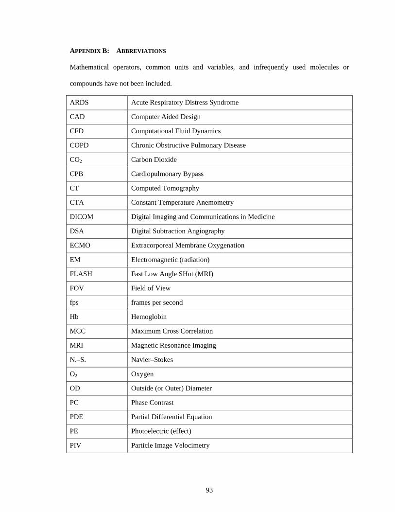
93
APPENDIX B: ABBREVIATIONS
Mathematical operators, common units and variables, and infrequently used molecules or
compounds have not been included.
ARDS Acute Respiratory Distress Syndrome
CAD Computer Aided Design
CFD Computational Fluid Dynamics
COPD Chronic Obstructive Pulmonary Disease
CO2 Carbon Dioxide
CPB Cardiopulmonary Bypass
CT Computed Tomography
CTA Constant Temperature Anemometry
DICOM Digital Imaging and Communications in Medicine
DSA Digital Subtraction Angiography
ECMO Extracorporeal Membrane Oxygenation
EM Electromagnetic (radiation)
FLASH Fast Low Angle SHot (MRI)
FOV Field of View
fps frames per second
Hb Hemoglobin
MCC Maximum Cross Correlation
MRI Magnetic Resonance Imaging
N.–S. Navier–Stokes
O2 Oxygen
OD Outside (or Outer) Diameter
PC Phase Contrast
PDE Partial Differential Equation
PE Photoelectric (effect)
PIV Particle Image Velocimetry

94
PMP Polymethylpentene
pps pixels per side
PTV Particle Tracking Velocimetry
RBC Red Blood Cell
ROI Region of Interest
SNR Signal to Noise Ratio

95
APPENDIX C: PSEUDO-LANGUAGE ALGORITHMS
Pseudo-Language Variables boxsz Template box dimensions corrlim Cross-correlation threshold limit
errvect Error vector properties (i.e., wrong direction, greater than local standard deviations, etc.)
frames Set of projection images gridsz Spatial discretization of grid points imdim Image dimensions img(–,a,b) Projection image (possible designation of specific biplane projection) N Loop counter NCC Normalized cross-correlation matrix nodes Vertices for spline construction
nx Normal direction of a point (i.e., inward or outward); default is positive (inward)
pcloud 3-D point cloud; includes xyz-coordinates and normal direction spline 2-D quasi-circular spline in z-plane splineres Spline resolution (number of points) tBox Template box thresh Background gray-level intensity tWin Search window winsz Search window dimensions Pseudo-Language Functions and Operations % Comment indicator : Range [] Omit, or remove value [·] Function parentheses (·) Contents, or subset of boundary Traces the boundary of a defined region (e.g., contrast bolus) count Count contents crop Remove matrix elements if, else Conditional statements max Maximum value rotate Rotate image run Execute, or evaluate search Search within domain(s) on which to evaluate a function smooth Spatial smoothing (i.e., median filter, hole filling, etc.) spline2d Execute 2-D cubic-spline interpolation stdev Standard deviation

96
C.1. Image Pre-Processing Subroutine
1. Input frames, imdim, thresh
2. Begin iteration of frames, N
3. Image pre-processing
img = rotate(img) % image alignment
img = crop(img) % remove known geometry
if, img(:,:) > thresh % binary image conversion
img(:,:) = 1
else, img(:,:) = 0
img = smooth(img)
4. [Enter Functions]
5. Repeat N
6. End N

97
C.2. Maximum Cross-Correlation
1. Input corrlim, errvect, gridsz, boxsz, winsz
2. Run C.1.
3. Calculate cross-correlation for each grid point
if, tBox(:,:) = boxsz % no calculations for a uniform
template pattern
else, NCC = search(tBox, tWin) % get max correlation
if, NCC(:,:) < corrlim, end
4. Refine NCC vectors
if, NCC(u,v) = errvect % sans standard deviation
NCC(u,v) = []
5. Only keep highest cross correlation for each grid point
NCC(N) = max(NCC(1:N))
6. Conduct filtering of final vector field
if, NCC(:,:) = errvect(stdev)
NCC(u,v) = []
7. Convert units: pixel/frame to mm/s

98
C.3. Point Cloud Reconstruction
1. Input splineres
2. Run C.1.
3. Identify outer edge of contrast perfusion
imga = boundary(imga)
imgb = boundary(imgb)
smooth(imga, imgb) % ensure continuous boundary (i.e., no
holes)
nodes = count(imga, imgb) % repeat for each row/slice
4. Refine nodes
if, nodes = 4 ∨ 12 % a slice must contain exactly 4 or 12
nodes; at least 2 from each img
if, [nodes = 4] ∧ [count(imga) = 2]
else, nodes = []
else, nodes = []
5. Create 2-D spline for each slice
spline = spline2d(nodes, splineres)
6. Export point cloud for volumetric reconstruction
pcloud = (nodes, slice, nx) % contains xyz-coordinates, and
normal direction
if, nodes = 4
else,
plcoud((2, 5, 8, 11),nx) = −nx % outward normal
(relative to inlet tube)

99
REFERENCES 1. Zwischenberger J, Vertrees R, Bedell E, McQuitty C, Chernin J, Woodson L.
Percutaneous Venovenous Perfusion-Induced Systemic Hyperthermia for Lung Cancer: A Phase I Safety Study. Ann Thorac Surg 2004;77:1916–25.
2. Conrad S, Zwischenberger J, Grier L, Alpard S, Bidani A. Total Extracorporeal Arteriovenous Carbon Dioxide Removal in Acute Respiratory Failure: A Phase I Clinical Study. Intens Care Med 2001;27:1340–51.
3. Zwischenberger J, Conrad S, Alpard S, Grier L, Bidani A. Percutaneous Extracorporeal Arteriovenous CO2 Removal for Severe Respiratory Failure. Ann Thorac Surg 1999;68:181–7.
4. Garcia J, Kon Z, Evans C, et al. Ambulatory Veno-Venous Extracorporeal Membrane Oxygenation: Innovation and Pitfalls. J Thorac Cardiov Surg 2011;142:755–61.
5. Xu J, Kochanek K, Murphy S, Tejada-Vera B. Deaths: Final data for 2007. Hyattsville, MD: National Center for Health Statistics; 2010.
6. OPTN / SRTR 2010 Annual Data Report. Rockville, MD: Department of Health and Human Services, Health Resources and Services Administration, Healthcare Systems Bureau, Division of Transplantation; 2011 January 4, 2012.
7. Organ Procurement and Transplantation Network (OPTN), 2012. (Accessed Jan 4, 2012, at http://optn.transplant.hrsa.gov/.)
8. Van Meurs K, Lally K, Peek G, Zwischenberger J, eds. ECMO Extracorporeal Cardiopulmonary Support in Critical Care. –3rd ed. Ann Arbor, MI: Extracorporeal Life Support Organization; 2005.
9. Wang D, Zwischenberger J, Chambers S. Artificial Gas Exchange. In: Eng Med Bio 27th Annual Conference; 2005; Shanghai, China: IEEE; 2005.
10. Zwischenberger J, Wang D, Lick S, Deyo D, Alpard S, Chambers S. The Paracorporeal Artificial Lung Improves 5-Day Outcomes From Lethal Smoke/Burn-Induced Acute Respiratory Distress Syndrome in Sheep. Ann Thorac Surg 2002;74:1011–8.
11. Haworth W. The Development of the Modern Oxygenator. Ann Thorac Surg 2003;76:S2216–9.
12. Iwahashi H, Yuri K, Nosé Y. Development of the Oxygenator: Past, Present, and Future. J Artif Organs 2004;7:111–20.
13. Lim M. The History of Extracorporeal Oxygenators. Anaesthesia 2006;61:984–95. 14. Sachs D, Derry G, Krumhaar D, Lee W, Maloney J. Chemical and Hypothermic
Inhibition of Intravascular Sludging in Extracorporeal Circulation. Ann Surg 1964;160:183–8.
15. Cohn L, ed. Cardiac Surgery in the Adult. –3rd ed. New York, NY: McGraw Hill Medical; 2008.
16. Wickramasinghe S, Han B, Garcia J, Specht R. Microporous Membrane Blood Oxygenators. AIChE J 2005;51:656–70.
17. Goerke A, Leung J, Wickramasinghe S. Mass and Momentum Transfer in Blood Oxygenators. Chem Eng Sci 2002;57:2035–46.
18. Niimi Y, Yamane S, Yamaji K, Tayama E, Sueoka A, Nosé Y. Protein Adsorption and Platelet Adhesion on the Surface of an Oxygenator Membrane. ASAIO J 1997;43:M706–10.

100
19. Shimono T, Shomura Y, Hioki I, et al. Silicone-Coated Polypropylene Hollow-Fiber Oxygenator: Experimental Evaluation and Preliminary Clinical Use. Ann Thorac Surg 1997;63:1730–6.
20. Shimono T, Shomura Y, Tahara K, et al. Experimental Evaluation of a Newly Developed Ultrathin Silicone Layer Coated Hollow Fiber Oxygenator. ASAIO J 1996;42:M451–4.
21. Koeppen B, Stanton B, eds. Berne and Levy Physiology. –6th ed. Philadelphia, PA: ELSEVIER; 2008.
22. Sherwood L, ed. Human Physiology: From Cells to Systems. –5th ed. Belmont, CA: Brooks/Cole–Thomson Learning; 2004.
23. West J, ed. Respiratory Physiology: The Essentials. –7th ed. Baltimore, MD: Lippincott Williams & Wilkins; 2005.
24. Lehle K, Alois P, Otto G, et al. Efficiency in Extracorporeal Membrane Oxygenation—Cellular Deposits on Polymethypentene Membranes Increases Resistance to Blood Flow and Reduce Gas Exchange Capacity. ASAIO J 2008;54:612–7.
25. Montoya J, Shanley C, Merz S, Bartlett R. Plasma Leakage through Microporous Membranes: Role of Phospholipids. ASAIO J 1992;38:M399–405.
26. Eash H, Jones H, Hattler B, Federspiel W. Evaluation of Plasma Resistant Hollow Fiber Membranes for Artificial Lungs. ASAIO J 2004;50:491–7.
27. LaFayette N, Schewe R, Montoya J, Cook K. Performance of a MedArray Silicone Hollow Fiber Oxygenator. ASAIO J 2009;55:382–7.
28. Kawahito S, Motomura T, Glueck J, Nosé Y. Development of a New Hollow Fiber Silicone Membrane Oxygenator for ECMO: The Recent Progress. Ann Thorac Cardiovasc Surg 2002;8:268–70.
29. Gartner M, Wilhelm C, Gage K, Fabrizio M, Wagner W. Modeling Flow Effects on Thrombotic Deposition in a Membrane Oxygenator. Artif Organs 2000;24:29–36.
30. Funakubo A, Taga I, McGilucuddy J, Fukui Y, Hirschl R, Bartlett R. Flow Vectorial Analysis in an Artificial Implantable Lung. ASAIO J 2003;49:383–7.
31. Snyder T, Eash H, Litwak K, et al. Blood Biocompatibility Assessment of an Intravenous Gas Exchange Device. Artif Organs 2006;30:657–64.
32. Wendel H, Philipp A, Weber N, Birnbaum D, Ziemer G. Oxygenator Thrombosis: Worst Case after Development of an Abnormal Pressure Gradient—Incidence and Pathway. Perfusion 2001;16:271–8.
33. Hoganson D, Anderson J, Weinberg E, et al. Novel Ambulatory Lung Assist Device Oxygenates and Removes Carbon Dioxide from Blood across a Silicone-Coated Porous Membrane. In: 16th Annual Surgical Resident and Fellow Research Presentation Day; 2009; Boston, MA: New England Surgical Society; 2009.
34. Verdonck P. The Role of Computational Fluid Dynamics for Artificial Organ Design. Artif Organs 2002;26:569–70.
35. Fill B, Gartner M, Johnson G, Horner M, Ma J. Computational Fluid Flow and Mass Transfer of a Functionally Integrated Pediatric Pump-Oxygenator Configuration. ASAIO J 2008;54:214–9.
36. Graefe R, Borchardt R, Arens J, Schlanstein P, Schmitz-Rode T, Steinseifer U. Improving Oxygenator Performance Using Computational Simulation and Flow Field-Based Parameters. Artif Organs 2010;34:930–6.
37. Goodin M, Thor E, Haworth W. Use of Computational Fluid Dynamics in the Design of the Avecor Affinity Oxygenator. Perfusion 1994;9:217–22.
38. Asakawa Y, Funakubo A, Fukunaga K, et al. Development of an Implantable Oxygenator with Cross-Flow Pump. ASAIO J 2006;52:291–5.
39. Mazaheri A, Ahmadi G. Uniformity of the Fluid Flow Velocities Within Hollow Fiber Membranes of Blood Oxygenation Devices. Artif Organs 2006;30:10–5.

101
40. Zhang J, Nolan T, Zhang T, Griffith B, Zhongjun J. Characterization of Membrane Blood Oxygenation Devices using Computational Fluid Dynamics. J Membr Sci 2007;288:268–79.
41. Sato H, Taga I, Kinoshita T, Funakubo A, Ichiba S, Shimizu N. In Vitro Evaluation of a Newly Developed Implantable Artificial Lung. Acta Med Okayama 2006;60:113–9.
42. Gage K, Gartner M, Burgreen G, Wagner W. Predicting Membrane Oxygenator Pressure Drop Using Computational Fluid Dynamics. Artif Organs 2002;26:600–7.
43. Poh C, Hardy P, Huang Z, Clark W, Gao D. Effect of Flow Baffles on the Dialysate Flow Distribution of Hollow-Fiber Hemodialyzers: A Nonintrusive Experimental Study Using MRI. J Biomed Eng 2003;125:481–9.
44. Ronco C, Brendolan A, Crepaldi C, Rodighiero M, Scabardi M. Blood and Dialysate Flow Distributions in Hollow-Fiber Hemodialyzers Analyzed by Computerized Helical Scanning Technique. J Am Soc Nephrol 2002;13:S53–61.
45. Patankar S. Numerical Heat Transfer and Fluid Flow. New York, NY: McGraw-Hill Book Co.; 1980.
46. McDonough JM, Lectures in Computational Fluid Dynamics of Incompressible Flow: Mathematics, Algorithms and Implementations. 2007. (Accessed January 17, 2011, at http://www.engr.uky.edu/~acfd/me691-lctr-nts.pdf.)
47. McDonough JM, Lectures in Basic Computational Numerical Analysis. 2007. (Accessed January 17, 2011, at http://www.engr.uky.edu/~acfd/me690-lctr-nts.pdf.)
48. Roache P. Quantification of Uncertainty in Computational Fluid Dynamics. Ann Rev Fluid Mech 1997;29:123–60.
49. Chen V, Li H, Fane A. Non-Invasive Observation of Synthetic Membrane Processes—A Review of Methods. J Membr Sci 2004;241:23–44.
50. Heese F, Robson P, Hall L. Quantification of Fluid Flow Through a Clinical Blood Filter and Kidney Dialyzer Using Magnetic Resonance Imaging. IEEE Sens J 2005;5:273–6.
51. Lu J, Lu W. Blood Flow Velocity and Ultra-Filtration Velocity Measured by CT Imaging System Inside a Densely Bundled Hollow Fiber Dialyzer. Int J Heat Mass Transfer 2010;53:1844–50.
52. Hirano A, Yamamoto K, Matsuda M, et al. Flow Uniformity in Oxygenators with Different Outlet Port Design. ASAIO J 2009;55:209–12.
53. Brownell L, Katz D. Flow of Fluids Through Porous Media 1: Single Homogeneous Fluids. Chem Eng Prog 1947;43:537–48.
54. Ergun S. Fluid Flow Through Packed Columns. Chem Eng Prog 1952;48:89–94. 55. Leva M. Fluidization. New York: McGraw-Hill Book Co.; 1959. 56. Chhabra R, Comiti J, Machač I. Flow of non-Newtonian Fluids in Fixed and Fluidised
Beds. Chem Eng Sci 2001;56:1–27. 57. Carman P. Fluid Flow Through Granular Beds. Trans Inst Chem Eng (London)
1937;15:150–66. 58. Dhotkar B, Chhabra R, Eswaran V. Flow of non-Newtonian Polymeric Solutions through
Fibrous Media. J Appl Polym Sci 2000;76:1176–85. 59. Herman P, Lehmann M, Velu Y. Predicting Initial Pressure Drop of Fibrous Filter
Media—Typical Models and Recent Improvements. JTATM 2006;5:1–15. 60. Jaganathan S, Tafreshi H, Pourdeyhimi B. A Realistic Approach for Modeling
Permeability of Fibrous Media: 3-D Imaging Coupled with CFD Simulation. Chem Eng Sci 2008;63:244–52.
61. Zobel S, Maze B, Tafreshi H, Wang Q, Pourdeyhimi B. Simulating Permeability of 3D Calendered Fibrous Structures. Chem Eng Sci 2007;62:6285–96.
62. Davies C. The Separation of Airborne Dust and Particles. Proc Inst Mech Eng 1952;1B:185–213.
102
63. Jackson G, Df J. The Permeability of Fibrous Porous Media. Can J Chem Eng 1986;64:364–74.
64. Niven R. Physical Insight into the Ergun and Wen & Yu Equations for Fluid Flow in Packed and Fluidised Beds. Chem Eng Sci 2002;57:527–34.
65. Dybbs A, Edwards R, eds. A New Look at Porous Media Fluid Mechanics. Darcy to Turbulent.: The Hague: Martinus Nijhoff; 1984.
66. Darcy H. Les Fontaines Publiques de la Ville de Dijon. Paris: Victor Delmont; 1856. 67. Bird R, Stewart W, Lightfoot E, eds. Transport Phenomena. –2nd ed.: John Wiley &
Sons, Inc.; 2007. 68. Pacella H, Eash H, Frankowski B, Federspiel W. Darcy Permeability of Hollow Fiber
Bundles used in Blood Oxygenation Devices. J Membr Sci 2011;382:238–42. 69. Burke S, Plummer W. Gas Flow through Packed Columns. Ind Eng Chem 1928;20:1196–
200. 70. ANSYS FLUENT 12.0 User’s Guide. In. Canonsburg, PA: ANSYS Inc.; 2009. 71. Macdonald T, El-Sayed M, Mow K, Dullien F. Flow through Porous Media—the Ergun
Equation Revisited. Ind Eng Chem Fundam 1979;18:199–208. 72. Dierickx P, de Wachter D, de Somer F, Van Nooten G, Verdonck P. Mass Transfer
Characteristics of Artificial Lungs. ASAIO J 2001;47:628–33. 73. Dierickx P, De Wachter D, Verdonck P. Blood Flow around Hollow Fibers. Int J Artif
Organs 2000;23:610–7. 74. Dupuit J. Études Théoriques et Practiques sur le Mouvement des Eaux dans les Canaux
Decouverts et á Travers les Terrains Perméables, 2nd ed. Paris, France: Dunod; 1863. 75. Civan F. Porous Media Transport Phenomena: John Wiley & Sons; 2011. 76. Duda A, Koza Z, Matyka M. Hydraulic Tortuosity in Arbitrary Porous Media Flow. Phys
Rev E 2011;84:036319. 77. Comiti J, Renaud M. A New Model for Determining Mean Structure Parameters of Fixed
Beds from Pressure Drop Measurements: Application to Beds Packed with Parallelepipedal Particles. Chem Eng Sci 1989;44:1539–45.
78. Vallabh R, Banks-Lee P, Seyam A. New Approach for Determining Tortuosity in Fibrous Porous Media. J Eng Fiber Fabr 2010;5:7–15.
79. Drummond J, Tahir M. Laminar Viscous-Flow Through Regular Arrays of Parallel Solid Cylinders. Int J Multiphase Flow 1984;10:515–40.
80. Ghaddar C. On the Permeability of Unidirectional Fibrous Media: A Parallel Computational Approach. Phys Fluids 1995;11:2563–86.
81. Liu S, Afacan A, Masliyah J. Steady Incompressible Laminar Flow in Porous Media. Chem Eng Sci 1994;49:3565–86.
82. Montillet A, Comiti J, Legrand J. Determination of Structural Parameters of Metallic Foams from Permeametry Measurements. J Membr Sci 1992;27:4460–4.
83. Ngo N, Tamma K. Microscale Permeability Predictions of Porous Fibrous Media. Int J Heat Mass Transfer 2001;44:3135–45.
84. Papathanasiou T, Markicevic B. A Computational Evaluation of the Ergun and Forchheimer Equations for Fibrous Porous Media. Phys Fluids 2001;13:2795–804.
85. Stylianopoulos T, Yeckel A, Derby J, et al. Permeability Calculations in Three-Dimensional Isotropic and Oriented Fiber Networks. Phys Fluids 2008;20:1–10.
86. Elsinga G, Scarano F, Wieneke B, van Oudheusden B. Tomographic Particle Image Velocimetry. Exp Fluids 2006;41:933–47.
87. Quénot G, Pakleza J, Kowalewski T. Particle Image Velocimetry with Optical Flow. Exp Fluids 1998;25:177–89.
88. Raffel M, Willert C, Wereley S, Kompenhans J, eds. Particle Image Velocimetry: A Practical Guide. –2nd ed. New York, NY: Springer; 2007.
89. Willert C, Gharib M. Digital Particle Image Velocimetry. Exp Fluids 1991;10:181–93.

103
90. Elkins C, Alley M. Magnetic Resonance Velocimetry: Applications of Magnetic Resonance Imaging in the Measurement of Fluid Motion. Exp Fluids 2007;43:823–58.
91. Uecker M, Zhang S, Voit D, Karaus A, Merboldt K, Frahm J. Real-Time MRI at a Resolution of 20 ms. NMR in Biomed 2010;23:986–94.
92. Bogunović H, Lončarić S. Blood Flow and Velocity Estimation Based on Vessel Transit Time by Combining 2D and 3D X-Ray Angiography. LNCS 2006;4191:117–24.
93. Castro M, Putman C, Cebral J. Patient-Specific Computational Modeling of Cerebral Aneurysms with Multiple Avenues of Flow from 3D Rotational Angiography Images. Acad Radiol 2006;13:811–21.
94. Dorsaz P, Doriot P, Dorsaz L, Chatelain P, Rutishauser W. A New Densiotometric Approach to the Assessment of Mean Coronary Flow. Invest Radiol 1997;32:198–204.
95. Moret J, Kemkers R, Op de Beek J, Koppe R, Klotz E, Grass M. 3D Rotational Angiography: Clinical Value in Endovascular Treatment. Medicamundi 1998;42:8–14.
96. Steinman D, Milner J, Norley C, Lownie S, Holdsworth D. Image-Based Computational Simulation of Flow Dynamics in a Giant Intracranial Aneurysm. Am J Neuroradiol 2003;24:559–66.
97. Waldenberger P, Chemelli A, Mallouhi A. Intra-Arterial Haemodynamic Changes during Cerebral Three-Dimensional Rotational Angiography. Eur Radiol 2009;19:503–8.
98. Cebral J, Pergolizzi R, Putman C. Computational Fluid Dynamics Modeling of Intracranial Aneurysms: Qualitative Comparison with Cerebral Angiography. Acad Radiol 2007;14:804–13.
99. Waechter I, Bredno J, Hermas R, Weese J, Barrat D, Hawkes D. Model-Based Blood Flow Quantification from Rotational Angiography. Med Image Anal 2008;12:586–602.
100. Shpilfoygel S, Close R, Valentino D, Duckwiler G. X-ray Videodensiotometric Methods for Blood Flow and Velocity Measurement: A Critical Review of Literature. Med Phys 2000;27:2008–23.
101. Gore J. Lectures in Medical Imaging. In. Nashville, TN: Vanderbilt University; 2006. 102. Dubsky S, Jamison R, Irvine S, Siu K, Hourigan K, Fouras A. Computed Tomographic
X-Ray Velocimetry. Appl Phys Lett 2010;96:1–3. 103. Heindel T, Gray J, Jensen T. An X-Ray System for Visualizing Fluid Flows. Flow Meas
Instrum 2008;19:67–78. 104. Irvine S, Paganin D, Jamison R, Dubsky S, Fouras A. Vector Tomographic X-Ray Phase
Contrast Velocimetry Utilizing Dynamic Blood Speckle. Opt Express 2010;18:2368–79. 105. Lee S, Kim G, Yim D, Jung S. Development of a Compact X-Ray Particle Image
Velocimetry for Measuring Opaque Flows. Rev Sci Instrum 2009;80:1–8. 106. Nikl M. Scintillation Detectors for X-Rays. Meas Sci Technol 2006;17:R37–54. 107. Zhao W, Rowlands J. X-Ray Imaging Using Amorphous Selenium - Feasibility of a Flat-
Panel Self-Scanned Detector for Digital Radiology. Med Phys 1995;22:1595–604. 108. Hoffmann K, Doi K, Fencil L. Determination of Instantaneous and Average Blood Flow
Rates from Digital Angiograms of Vessel Phantoms Using Distance-Density Curves. Invest Radiol 1991;26:207–12.
109. Tenjin H, Asakura F, Nakahara Y, Matsumoto K, Matsuo T. Evaluation of Intraaneurysmal Blood Velocity by Time-Density Curve Analysis and Digital Subtraction Angiography. Am J Neuroradiol 1998;19:1303–7.
110. Harrington D, Boxt L, Murray P. Digital Subtraction Angiography—Overview of Technical Principles. Am J Roentgenol 1982;139:781–6.
111. Meijering E, Niessen W, Viergever M. Retrospective Motion Correction in Digital Subtraction Angiography: A Review. IEEE Trans Med Imaging 1999;18:2–21.
112. Kersten M, Stewart A, Troje N, Ellis R. Enhancing Depth Perception in Translucent Volumes. IEEE Trans Visual Comput Graphics 2006;12:1117–23.
104
113. Hardy J, Dodds S, Roberts A. An Objective Evaluation of the Effectiveness of Different Methods of Displaying Three-Dimensional Information with Medical X-Ray Images. Invest Radiol 1996;31:433–45.
114. Talukdar A, Wilson D. Modeling and Optimization of Rotational C-Arm Stereoscopic X-Ray Angiography. IEEE Trans Med Imaging 1999;18:604–16.
115. Pellot C, Herment A, Sigelle M, Horain P, Maitre H, Peronneau P. A 3D Reconstruction of Vascular Structures from Two X-Ray Angiograms using an Adapted Simulated Annealing Algorithm. IEEE Trans Med Imaging 1994;13:48–60.
116. Pellot C, Herment A, Sigelle M, Horain P. Segmentation, Modelling and Reconstruction of Arterial Bifurcations in Digital Angiography. Med & Biol Eng & Comput 1992;30:576–83.
117. Prause G, Onnasch D. Binary Reconstruction of the Heart Chambers from Biplane Angiographic Image Sequences. IEEE Trans Med Imaging 1996;15:532–46.
118. Seeger A, Kertzscher U, Affeld K, Wellnhofer E. Measurement of the Local Velocity of the Solid Phase and the Local Solid Hold-Up in a Three-Phase Flow by X-ray Based Particle Tracking Velocimetry (XPTV). Chem Eng Sci 2003;58:1721–9.
119. Song S, Leahy R. Computation of 3-D Velocity Fields from 3-D Cine CT Images of a Human Heart. IEEE Trans Med Imaging 1991;10:295–306.
120. Schmitt H, Grass M, Suurmond R, et al. Reconstruction of Blood Propagation in Three-Dimensional Rotational X-Ray Angiography (3D-RA). Comput Med Imag Grap 2005;29:507–20.
121. Pratt W, ed. Digital Image Processing: PIKS Inside. –3rd ed.: John Wiley & Sons, Inc; 2001.
122. Condell J, Scotney B, Morrow P. The Effect of Presmoothing Image Sequences on the Computation of Optical Flow. Lect Notes in Comput Sci 2006;4141:780–91.
123. Dransfeld S, Larnicol G, Yves Le Traon P. The Potential of the Maximum Cross Correlation Technique to Estimate Surface Currents from Thermal AVHRR Global Area Coverage Data. IEEE Geosci Remote Sens Lett 2006;3:508–11.
124. Bowen M, Emery W, Wilkin J, Tildesley P, Barton I, Knewtson R. Extracting Multiyear Surface Currents from Sequential Thermal Imagery Using the Maximum Cross-Correlation Technique. J Atmos Oceanic Technol 2002;19:1665–76.
125. Crocker R, Matthews D, Emery W, Baldwin D. Computing Costal Ocean Surface Currents from Infrared and Ocean Color Satellite Imagery. IEEE Trans Geosci Remote Sens 2007;45:435–47.
126. Lewis J. Fast Normalized Cross-Correlation. Vision Interface 1995. 127. Cattaneo G, Reul H, Schmitz-Rode T, Steinseifer U. Intravascular Blood Oxygenation
Using Hollow Fibers in a Disk-Shaped Configuration: Experimental Evaluation of the Relationship Between Porosity and Performance. ASAIO J 2006;52:180–5.
128. Baurmeister U, inventor Akzo NV, Arnhem, Netherlands, assignee. Multilayer Hollow Fiber Wound Body. United States patent 5,143,312 Sep. 1, 1992.
129. Jönsson K, Jönsson B. Fluid-Flow in Compressible Porous Media I: Steady-State Conditions. AIChE J 1992;38:1340–8.
130. Cook K, Maxhimer J, Leonard D, Mavroudis C, Backer C, Mockros L. Platelet and Leukocyte Activation and Design Consequences for Thoracic Artificial Lungs. ASAIO J 2002;48:620–30.
131. Gu Y, Boonstra P, Graaff R, Rijnsburger A, Mungroop H, van Oeveren W. Pressure Drop, Shear Stress, and Activation of Leukocytes During Cardiopulmonary Bypass: A Comparison Between Hollow Fiber and Flat Sheet Membrane Oxygenators. Artif Organs 2000;24:43–8.
132. Kroll M, Hellums J, McIntire L, Schafer A, Moake J. Platelets and Shear Stress. Blood 1996;88:1525–41.

105
133. Runyon M, Kastrup C, Johnson-Kerner B, Van Ha T, Ismagilov R. Effects of Shear Rate on Propagation of Blood Clotting Determined Using Microfluidics and Numerical Simulations. JACS 2008;130:3458–64.
134. Goodman P, Barlow E, Crapo P, Mohammad S, Solen K. Computational Model of Device-Induced Thrombosis and Thromboembolism. Ann Biomed Eng 2005;33:780–97.
135. Leverett L, Hellums J, Alfrey C, Lynch E. Red Blood Cell Damage by Shear Stress. Biophys J 1972;12:257–73.
136. Brooks D, Goodwin J, Seaman G. Interactions among Erythrocytes under Shear. J Appl Physiol 1970;28:172–7.
137. Sun C, Migliorini C, Munn L. Red Blood Cells Initiate Leukocyte Rolling in Postcapillary Expansions: A Lattice Boltzmann Analysis. Biophys J 2003;85:208–22.
138. Guan Y, Palanzo D, Kunselman A, Ündar A. Evaluation of Membrane Oxygenators and Reservoirs in Terms of Capturing Gaseous Microemboli and Pressure Drops. Artif Organs 2009;33:1037–43.
139. Rayz V, Boussel L, Lawton M, et al. Numerical Modeling of the Flow in Intracranial Aneurysms: Prediction of Regions Prone to Thrombus Formation. Ann Biomed Eng 2008;36:1793–804.
140. Chan K, Fujioka H, Bartlett R, Hirschl R, Grotberg J. Pulsatile Flow and Mass Transport Over an Array of Cylinders: Gas Transfer in a Cardiac-Driven Artificial Lung. J Biomech Eng 2006;128:85–96.
141. Zierenberg J, Fujioka H, Cook K, Grotberg J. Pulsatile Flow and Oxygen Transport Past Cylindrical Fiber Arrays for an Artificial Lung: Computational and Experimental Studies. J Biomech Eng 2008;130:031019:1–12.
142. Shibeshi S, Collins W. The Rheology of Blood Flow in a Branched Arterial System. Appl Rheol 2005;15:398–405.
143. Venkataraman P, Rama Mohan Rao P. Darcian, Transitional, and Turbulent Flow Through Porous Media. J Hydraul Eng 1998;124:840–6.

106
VITA
CAMERON C. JONES
Current Positions 8/2011–Present Research Engineer I, Exatherm LLC, Lexington, Kentucky 1/2010–Present R&D Engineer, Therix Medical Inc., Lexington, Kentucky Previous Positions 6/2005–4/2007 Research Assistant in Medical Imaging, Vanderbilt University,
Nashville, Tennessee 5/2004–4/2007 Research Assistant in Radiation and Radiation Oncology, Vanderbilt
University, Nashville, Tennessee Education 2003–2007 B.E. Biomedical Engineering, Vanderbilt University; Nashville,
Tennessee Certifications 2007–Present Engineering Intern, Tennessee Board of Architectural and Engineering
Examiners (Certification No. 26250)
Publications (Peer Reviewed) 1. De Bartolo C, Nigro A, Fragomeni G, Colacino FM, Wang D, Jones CC, and
Zwischenberger JB. (2011). “Numerical and Experimental Flow Analysis of the Wang-Zwische Double Lumen Cannula.” ASAIO, 57(4):318–27.
2. Huamani J, Willey C, Dinesch T, Niermann KJ, Reyzer M, Leavitt LL, Jones CC, Fleischer AC, Caprioli R, Hallahan DE, and Kim DW. (2008). “Differential Efficacy of Combined Therapy with Radiation and AEE788 in High and Low EGFR-Expressing Androgen-Independent Prostate Tumor Models.” Int J Radiat Oncol Biol Phys, 71:237–46.
3. Kim DW, Huamani J, Niermann KJ, Lee H, Geng L, Leavitt LL, Baheza RA, Jones CC, Tumkur S, Yankeelov TE, Fleischer AC, and Hallahan DE. (2006). “Noninvasive Assessment of Tumor Vasculature Response to Radiation-Mediated, Vasculature-Targeted Therapy Using Quantified Power Doppler Sonography.” J Ultrasound Med, 25:1507–17.
Publications (In Preparation)
1. Jones CC, Capasso P, Wang D, McDonough JM, Rosenstein KS, and Zwischenberger JB. “Biplane Angiography for Experimental Validation of CFD Models of Blood Flow in Artificial Lungs.” Submitted.
2. Ballard-Croft C, Wang D, Jones CC, Zhou X, Sumpter LR, and Zwischenberger JB. “A New, Simplified Systemic Hyperthermia Circuit for Advanced Lung Cancer Treatment.” Submitted.
Book Chapters
1. Niermann KJ, Fleischer AC, Jarquin-Valdivia A, Jones CC, Lefkovitz E, Donnelly E, and Martin DS. (2004). “Sonographic Assessment of Skeletal Muscles: Implications for a Manned Mission to Mars.” In DF Crossman & DR Zubrin (Eds.), On To Mars 2—Exploring and Settling a New World (Vol. 55). Burlington, Ontario: Apogee Books Space Series.

107
Presentations 1. Croft C, Wang D, Jones CC, Rosenstein K, Sumpter LR, Zhao J, Zhou X, and
Zwischenberger JB. (2012). “Five Day Preclinical Sheep Studies Using a New Venovenous Perfusion-Induced Systemic System Hyperthermia Circuit.” ASAIO 58th Annual Conference, San Francisco, CA.
2. Jones CC, Capasso P, Wang D, McDonough JM, and Zwischenberger JB. (2011). “Using Biplane Angiography to Validate Computational Fluid Dynamic Models of Blood Flow in Artificial Lungs.” ASAIO 57th Annual Conference, Washington, DC.
3. Wang D, Plunkett M, Zhou X, Rosenstein K, Jones CC, Bacchetta M, and Zwischenberger J. (2011). “Development of a Percutaneous Double Lumen Cannula for Ambulatory Right Heart Support.” ASAIO 57th Annual Conference, Washington, DC.
4. Wang D, Plunkett M, Croft C, Zhou X, Rosenstein K, Jones CC, and Zwischenberger J. (2011). “A Percutaneous OxyRVAD for Lung and Right Heart Support.” ASAIO 57th Annual Conference, Washington, DC.
5. Croft C, Wang D, Jones CC, Thomas J, Rosenstein K, and Zwischenberger J. (2010). “A New Venovenous Perfusion-Induced Systemic Hyperthermia Circuit for Advanced Lung Cancer.” ASAIO 56th Annual Conference, Baltimore, MD.
6. Jones CC. (2010). “Design in the Biomedical Industry.” Biomedical Engineering Seminar Series, Lexington, KY.
7. Jones CC, Wang D, Zwischenberger JB. (2009). “Thrombosis in Membrane Oxygenators.” Biomedical Engineering Seminar Series, Lexington, KY.
Posters
1. Ballard-Croft C, Wang D, Jones CC, Sumpter LR, Zhou X, Thomas J, and Zwischenberger JB. (2012). “Physiological Response to a Simplified Venovenous Perfusion-Induced Systemic Hyperthermia System.” ASAIO 58th Annual Conference, San Francisco, CA.
2. Croft C, Wang D, Jones CC, Thomas J, Rosenstein K, and Zwischenberger J. (2011). “A New Venovenous Perfusion-Induced Systemic Hyperthermia Circuit for Advanced Lung Cancer.” University of Kentucky Markey Cancer Research Day Annual Conference, Lexington, KY.
3. Blyth C, Fernandez C, Hittinger S, Jones CC, McGee B, Kam T, and Wood B. (2007). “Cauterization Catheter – An Advancement in Conductive Biomaterials and Medicine.” Vanderbilt University Senior Design Project Presentations, Nashville, TN.
4. Jones CC, Stepniewska I, and Anderson AW. (2006). “A Simple Optical Tracking Technique to Classify Forelimb Motion Evoked by Cortical Stimulation.” Vanderbilt University Independent Research Presentations, Nashville, TN.
5. Kim DW, Huamani J, Niermann KJ, Lee H, Geng L, Leavitt L, Baheza R, Jones CC, Tumkur S, Yankeelov TE, and Hallahan DE. (2006). “Schedule Optimization of Ablative Radiation Treatments Based on Physiologic Parameters of Response.” Vanderbilt University Research Forum Annual Conference, Nashville, TN.
6. Huamani J, Niermann KJ, Reyzer ML, Alberts J, Jones CC, Caprioli R, Hallahan DE, and Kim DW. (2005). “Combination Therapy of Ionizing Radiation with AEE788, a Dual Receptor Tyrosine Kinase Inhibitor Targeting Epidermal Growth Factor Receptor (EGFR) and Vascular Endothelial Growth Factor Receptor (VEGFR) Leads To Improved Tumor Control.” Vanderbilt Ingram Cancer Center Annual Conference, Nashville, TN.