validation of a phenomenological model for the state ... · validation of a phenomenological model...

VII CAIQ 2013 y 2das JASP

AAIQ Asociación Argentina de Ingenieros Químicos - CSPQ

VALIDATION OF A PHENOMENOLOGICAL MODEL FOR THE

STATE VARIABLES IN THE NON-ISOTHERMAL WINE

FERMENTATION

P. M. Aballaya*, G. J. E. Scaglia

a, M. D. Vallejo

b, O. A. Ortiz

a, M. E. Serranoª, C. A.

Menguala, S. Rómoliª.

ª Instituto de Ingeniería Química, b

Instituto de Biotecnología

(Universidad Nacional del San Juan – Facultad de Ingeniería)

Av. Lib. San Martín (Oeste) 1109 - J5400ARL San Juan - Argentina

E-mail: [email protected]

Abstract. In winemaking, fermentation kinetics is temperature-dependent.

Also, quality, quantity and rate of aroma compounds may be “fine-tuned”

by manipulating the temperature. Hence, oenologists use variable

temperature profiles during the fermentation, to obtain high-quality varietal

wines. This non-isothermal batch operation must be carefully controlled to

avoid sluggish or stuck fermentations and favor the appearance of the

preferred sensory features: acidity, ethanol level, and sugar depletion.

Isothermal mathematical models cannot be used for controlling these

bioprocesses. So, more rigorous and accurate models are necessary. This

work proposes an improved non-isothermal phenomenological model for

the alcoholic fermentation step in winemaking that considers temperature as

the most critical variable influencing the mentioned bioprocess. The

developed model, based on previous ones published by authors, couples

mass and energy balances between the reactor and its cooling jacket. It

predicts viable cells, total fermentable sugars and ethanol concentrations,

carbon dioxide released on bioreactor temperature. It is considered a new

expression depending on temperature for: maximum specific cellular growth

* A quien debe enviarse toda la correspondencia

mailto:[email protected]


AAIQ, Asociación Argentina de Ingenieros Químicos - CSPQ

and death rates, and the carbon dioxide released at 85-95% of its maximum

value. The model has been validated, with an adequate accuracy, by own

lab-scale fermentations and by data from literature for the four state

variables of the process. Simulations at different constant temperatures and

for predefined temperature trajectories, between 10 - 40ºC, were performed.

Given that attained results are suitable, this model can be used to track

complex temperature profiles to obtain high-quality wines, and in control

and optimization strategies as well.

Keywords: Non-isothermal operation, Alcoholic wine fermentation, First-

principles model.

1. INTRODUCTION

Argentina is the largest wine producer in South America. In the last years, the range

of varietal wines has increased their penetration into the most important international

consumers markets. Some of such wines are among the top rated wines in the world.

The customers’ increasing demand for high quality wines and its marked preferences for

wines with outstanding organoleptic properties, presents new challenges for the

winemaking technology.

The bioreactor bulk temperature is a well-known critical variable that determine the

kinetics of the fermentation (Coleman et al., 2007). This operation variable directly

influences on microbial ecology of grape must and the biochemical reactions of yeasts

(Fleet & Heard, 1993). Moreover, it is known that Saccharomyces cerevisiae

synthesizes aroma compounds during the winemaking fermentations. It is also stated

that the production, quality, quantity and rate of yeast-derived aroma compounds is

affected by the temperature used. Usually, temperatures ranging between 15ºC (for

white wines) and 30ºC (for red wines) are used. Furthermore, most winemaking

fermentations are not carried out at constant temperature. Experiments conducted at

constant temperature, revealed that production of compounds related to fresh and fruity



aromas is favored at temperatures near 15°C, while flowery related aroma compounds

are better produced at 28°C (Molina et al., 2007).

With respect to some sensory-relevant flavor generation, it was suggested that higher

temperatures, near 28 ºC, are only beneficial at the start of fermentation, and then lower

temperatures will be advantageous due to the decrease of the volatility and removal of

the aroma compounds formed (Fischer, 2007).

It is evident that temperature strongly affects the quality of wine (Torija et al., 2003),

and new technologies must include variable temperature trajectories (profiles)

throughout the fermentation. Therefore, the development of efficient control strategies

for the main operation variables in fermentations such as pH, temperature, dissolved

oxygen concentration; agitation speed, foam level, and others need accurate dynamic

models (Morari & Zafiriou, 1990, Henson, 2003, Ortiz et al., 2009, Sablayrolles, 2009).

Also, wine fermentation models, with process control purposes, are useful tools to

assure wine quality and reproducibility among batches (Zenteno et al., 2010).

In previous reports, the authors have developed isothermal and non-isothermal first-

principles and hybrid neural models, and an improved isothermal phenomenological

model with satisfactory capability to approximate the wine fermentation profiles

(Vallejo et al., 2005, Ortiz et al., 2006, Aballay et al., 2008, Scaglia et al., 2009).

This work propose a continuation of the non-isothermal phenomenological model for

wine fermentation kinetics developed previously, but in this case, able to predict the

main bioprocess state variables: viable cells, substrate and ethanol concentrations, and

carbon dioxide released and track complex temperature profiles from 10 to 40ºC with

adequate rigor, to produce high quality varietal wines.

The model couples mass and energy balances predicting the behavior of the main

state process variables: viable cells, substrate (total fermentable sugars) and ethanol

concentrations, carbon dioxide released, and the bioreactor temperature. It is based with

modifications on the one developed by (Scaglia et al., 2009) that possesses a good

performance for isothermal fermentations, and the ones presented by (Aballay et al.,

2008, Aballay et al., 2010, Aballay et al., 2012) for non-isothermal fermentations with

temperature ranges from 20 to 30ºC, in the first case, and 10 to 40°C in the remaining

cases, predicting ethanol level additionally to the viable cells evolution during



fermentation, in the latter case. Balances are represented by a set of ordinary differential

equations (ODE), including the heat transferred between the reactor and its cooling

jacket. Moreover, balances have been coupled by means of the Arrhenius equation

describing temperature influence on the cell growth (Aballay et al., 2006, Aballay et al.,

2008) and death rates (Phisalaphong et al., 2006), and the kinetic parameter of the

model of (Scaglia et al., 2009): carbon dioxide released at 85-95% of its maximum

value.

Kinetic parameters of the model were adjusted using experimental data obtained

from anaerobic lab-scale cultures of S. cerevisiae (killer), and/or Candida cantarellii

yeasts in Syrah must (red-grape juice), see (Toro & Vazquez, 2002). In the case of the

specific parameters in Arrhenius expression, they were adjusted by the least-square

method.

In practice, the temperature in the bioreactor must be maintained constant at a certain

level to avoid the quality product decrease, or varied tracking a predefined trajectory to

achieve a varietal wine with particular organoleptic properties (Ortiz et al., 2009). Thus,

the model performance was tested via simulation to validate it. Results from model

simulations and validation are shown. They state suitable agreement with own

experimental and published data, which allows the model to predict without significant

retards the fermentation evolution. The latter permit model application in advanced

control and optimization strategies for the winemaking process.

The work is organized as follows. First, the lab-scale fermentation experiments,

carried out with variable temperature to validate the model, are described. Second, the

non-isothermal kinetic modeling of the bioprocess is presented. Third, model simulation

results are compared to: literature data to verify they well track process state variables

and, own experimental data for its validation. Fourth, a discussion on the possible use of

the obtained model in complex control and optimization schemes in winemaking, and

conclusions are exposed.

2. MATERIALS And METHODS

Microorganism: Saccharomyces cerevisiae, (strain PM16, obtained in our

laboratory), maintained in agar-YEPD (yeast extract-peptone-dextrose), and propagated



in red-grape must. Culture medium: concentrated red-grape must, properly diluted to

obtain 23ºBrix at 23ºC, initial pH was set to 3.5, and sterilized at 121ºC during 20

minutes. Fermentations (FERC): 250 mL flasks containing 100 mL of sterile must was

inoculated with 3x106 yeasts, capped with Muller’s valves, and cultured in anaerobic

conditions, at temperature following the sequence from 23ºC to 18ºC, presented in Fig.

3. Samples were taken each 6 hours during the first 7 days and then each day; yeasts

were accounted by means a Neubauer chamber, the fermented must was centrifuged and

the supernatant was maintained for sugar (by spectrophotometric method) and ethanol

(by distillation) determinations.

3. MATHEMATICAL MODELLING

In winemaking conditions, the main bio-reactions can be synthesized by the

reductive pathway S X + P + CO2, this reaction means that substrates (S, glucose and

fructose and sucrose, after their hydrolysis as the limiting substrate), in anaerobic

conditions, are metabolized to produce a yeast population (X), ethanol (P, mainly

produced by yeast through the Embden-Meyerhof-Parnas metabolic pathway) and

carbon dioxide (CO2).

The ethanol-formation reaction from glucose is:

6 12 6 3 2 22 2C H O CH CH OH CO (1)

The metabolite accumulation in the extra-cellular medium has been modeled by a set

of ODE based on mass balances on X, S, P and CO2 which change with time t [h] like in

the isothermal model of (Scaglia et al., 2009), which can be seen for further details with

some modifications expressed in point 4 (sensitivity analysis), and it is summarized as

Eqs. (2) through (5):

Viable cells:



2 2(95)

2 2(95) 2 2(95)

2 2(95)

2 2(95) 2 2(95)

( 0 )

m( 0 ) ( 0 )

m

( 0 )

( 0 ) ( 0 )

1

( )

1

CO C

CO C CO C

CO C

dCO C CO C

dX e S XA X

Sdt S Ks B ae e AS Ks B a

e dSC X K X

dte e

(2)

Substrate:

m

/

1X FX

X S

dS SX E

dt Y S Ks Bb

(3)

Carbonic anhydride:

2

m

dCO S dG X I X

dt S Ks Bc dt

(4)

Ethanol:

2

2

/

1

CO P

dCOdP

dt Y dt

(5)

Numerical values of previous model parameters and their description are shown in

Table 1.

Model assumptions are: other mass balance parameters of the model, including pH,

are constant. Fermentation is not nitrogen source-limited; this is viable, based on

information about the chemical composition of the local red-grape musts. Moreover,

local winemakers only add nitrogen supplementation, in excess, to correct the white-

grape musts. In the energy balance Eq. (6): heat losses due to CO2 evolution, water

evaporation and ethanol and flavor losses are neglected; the average grape juice-wine

density and specific heat, and all physical properties are uniform in the fermenting mass

bulk. They are constant with the (bioreactor) temperature T [K] and time. Convective

heat transfer coefficient of fermentation mass, implicitly included in Eq. (6), is constant



(Colombié et al., 2007). In the cooling jacket side: water properties variations and the

fouling factor are neglected. Heat transfers by radiation and conduction are negligible.

Table 1. Coefficients and parameters values from the isothermal fermentation model

of (Scaglia et al., 2009), used in the present non-isothermal model for three

fermentations.

Fitting coefficient

Description Unit Value

FERA

FERC FERB

a - - 0.1228 1.8284 1.1666

b - - 1.000 0.5115 1.000

c - - 1.281 1.4846 1.1666

d - - 1.152 1.152 1.152

e - - 1.355 1.355 1.355

A - - 3.119 8.27 5.622

B Coefficient related to ethanol-

tolerance - 178.945 278.984 278.984

C Volume of fermenting mass per

substrate mass m

3 kg

-1 8∙10

-4 0.001 0.001

E Volume of fermenting mass per

formed cells and time

m3 kg

-1

hr-1

1.65∙10-

4 2.88∙10

-

5

9.89∙10-

5

F

Specific rate of substrate

consumption for cellular

maintenance

kg kg-1

hr-1 0.012 0.009 0.007

G CO2 released per formed cells kg kg-1

10.091 49.002 13.2

I Similar to G kg kg-1

1.8 (-8.46) 0.3

Ks Saturation coefficient in

Monod’s equation kg m

-3 2.15 2.15 2.15

Coefficient in Verlhurst’s

equation

m3 kg

-1

h-1 4.5∙10

-3 3.2∙10

-3 3.1∙10

-3

YX/S Formed cells per consumed

substrate kg kg

-1 0.04 0.061 0.0152

YCO2/P Carbon dioxide yield

coefficient based on ethanol kg kg

-1 0.775 0.998 1.054



The non-isothermal kinetic model is constituted by mass balances of the before-

mentioned model and the energy balance in the reactor and its cooling water jacket.

2

2

/

r r r

H CO r

d V Cp T dCOY V Q

dt dt

(6)

Vr [m3] is the volume. YH/CO2 [W·h produced/kg CO2 released] is the energy due to

the carbon dioxide released by the bio-reaction. It was obtained by stoichiometry Eq. (1)

from YH/S, the likely energetic yield on substrate consumed during the bio-reaction. Q

[W] represents the exchanged heat between the fermenting mass and the cooling jacket

(see details in Aballay et al.( 2008)). ρr [kg m-3] and Cpr [W·h kg-1

K-1

] are density and

specific heat of the fermenting mass.

Mass and energy balances are coupled by means of: Arrhenius equation for

maximum specific cellular growth and death rates, m [h-1

] and Kd [h-1

] respectively,

and polynomial regressions for dimensionless coefficients L within m, and M within

the parameter for estimation of the carbon dioxide released at 85-95% of its maximum

value CO2(95). The above mentioned bioprocess variables progress in time and,

temperature influence on them and their parameters can be expressed in a general way

as: 2 2 2(95), , , ( , , , ( ), ( ), ( )).m ddX dt dS dt dCO dt dP dt f X S CO T K T CO T

The mathematical expressions for the three kinetic temperature-dependent

parameters are given in Eqs. (7), (8) and (9):

. .

1

a

d

E

R T

m G

R T

T eL

e

(7)

is the maximum cellular growth rate per Kelvin degree [h-1

K-1

], L is a

dimensionless coefficient depending on the temperature Eq. (10), Ea is the activation

energy for cell growth [kJ kmol-1

] and Gd [kJ kmol-1

] is Gibbs free energy change of

the fermentation reaction. R is general gases constant [kJ kmol-1

K-1

].



,0 304dE

R Td

dK T e if T KK

0.0165 Otherwise

(8)

Kd replaces parameter D in the model of (Scaglia et al., 2009). Kd,0 is the specific

cellular death rate per Kelvin degree and Ed is the activation energy for cellular death

[kJ kmol-1

].

Moreover, parameters Ea, Gd, Kd,0, and Ed, were adjusted by the least-square

method, using experimental data obtained from anaerobic lab-scale cultures of S.

cerevisiae (killer) and C. cantarellii yeasts, with Syrah must in batch mode (Toro &

Vazquez, 2002).

*

2(95) 2(95)CO CO M (9)

CO*2(95) is a carbon dioxide value, chosen between the 85% and 95% of the total

carbon dioxide released at constant temperature (296 K) and, M is a dimensionless

coefficient depending on the temperature Eq. (11).

5 4 3 2T - g T + h T - i T + j T - kL f (10)

5 4 3 2T - m T + n T - o T + p T - qM l (11)

Where f, g, h, i, j, k, l, m, n, o, p, and q are own coefficients of the model, see Table

2. Other parameters values of the model are included in Table 2.

Initial conditions used for simulating own and from literature experimental

fermentations are resumed in Figures (1-3) captions. Those fermentations are

mentioned as: FERA and FERB (Toro & Vazquez, 2002) and FERC from own data.

The latter was carried out to validate the present model. In addition, maximum values of

viable cells concentration achieved during the fermentations are included in Figures (1-

3) captions.



Table 2. Coefficients and parameters used in the proposed non-isothermal model for

three fermentations.

Fitting coefficient

Description Unit Value

FERA FERC FERB

f - - 4.23∙10-7 4.23∙10-7 4.23∙10-7

g - - 6.41∙10-4 6.41∙10-4 6.41∙10-4

h - - 0.3873 0.3873 0.3873

i - - 116.9 116.9 116.9

j - - 17631 17631 17631

k - - 1.06∙106 1.06∙106 1.06∙106

l - - 2.7∙10-7 2.7∙10-7 2.7∙10-7

m - - 4.1∙10-4 4.1∙10-4 4.1∙10-4

n - - 0.2479 0.2479 0.2479

o - - 74.89 74.89 74.89

p - - 11299 11299 11299

q - - 6.81∙105 6.81∙105 6.81∙105

Physical-chemical and kinetic parameters

ρr Density of the fermenting mass kg m-3 1020.948 1020.94

8

1020.948

Cpr Specific heat of the fermenting

mass

W·h kg-1 K-1 1.01684 1.01684 1.01684

Vr Volume of the fermenting mass m3 0.003 0.003 0.003

YH/CO

2

Energy due to the carbon

dioxide released by the bio-

reaction

W·h

produced/kg

of CO2

released

310.3748

310.374

8

310.3748

Maximum cellular growth rate

per Kelvin degree

h-1K-1 1.66 0.3766 1.08

Gd Gibbs free energy change of the

fermentation reaction

kJ kmol-1 1916.9 1916.9 1916.9

Ea Activation energy for cell

growth

kJ kmol-1 1928.37 1928.37 1928.37

Ed Activation energy for cell death kJ kmol-1 1.789∙105 1.789∙105

1.741∙105

Kd,0 Specific cellular death rate per

Kelvin degree

h-1 K-1 1.3∙1027 1.2∙1027 4.16∙1025

*

2(95)CO

CO2 released between 85-95%

of the maximum CO2 released

at constant temperature

kg m-3 97.5 97.5 94

R General gases constant kJ kmol-1 K-1 8.309 8.309 8.309



4. SIMULATIONS

4.1 RESULTS

The developed model was tested via simulations in similar conditions than

experimental fermentations from literature. To carry out the simulations, the model was

codified in MatlabTM

(2008) software.

In order to contrast the simulation results obtained with experimental data from

literature, please see reported experiences of wine fermentations at different constant

initial temperatures (Torija et al., 2003) and the 3D-mesh plot in the work of Aballay et

al. (2010).

4.2 MODEL VALIDATION

The model validation was accomplished by simulation as well, using initial

conditions of different own lab-scale experimental data sets at different constant

temperatures and at variable temperature profiles. Fig. 1 shows that for fermentations

FERA and B (both at constant 296±1 K), the model proposed has an adequate

prediction: (FERA) with only up to 13.5 hours average in advance with respect to

experimental P, and up to 11.7 hours average in retard, with respect to experimental

CO2, (FERB) with only up to 14.5 hours average in advance with respect to

experimental P, and up to 16 hours average in retard with respect to experimental CO2.

0 50 100 150 200 250 300 350 400 450 5000

50

100

150

200

250

Time [h]

P, C

O2

, S

[kg m

-3]

Modelled P

Experimental P

Modelled S

Modelled CO2

Experimental CO2

a

0 50 100 150 200 250 300 350 400 450 5000

50

100

150

200

250

Time [h]

P, C

O2

, S

[kg m

-3]

Modelled P

Experimental P

Modelled S

Modelled CO2

Experimental CO2

b

Fig. 1. Ethanol concentration / CO2 profiles: modeled and experimental fermentations, also modeled substrate

concentration: (a) FERA (Xmax. = 92.3∙106 cfu mL-1) and (b) FERB (Xmax. = 109.74∙106 cfu mL-1), both of them at

296±1K and with initial: S(0) = 208.5 kg m-3, X(0) = 2∙106 cfu mL-1.



Figure (2a), presents the model predictions and experimental results for fermentation

FERC performed at a predefined temperature profile, Fig. (2b), fixed from biochemical

considerations on yeasts growth and yeast-related aroma compounds. Fig. (2a), shows

that the model proposed has an acceptable prediction for P and CO2 as well, with only

up to 15 hours average in retard with respect to experimental P, up to 24 hours average

in advance, with respect to experimental CO2.

0 50 100 150 200 250 300 350 400 450 5000

50

100

150

200

250

Time [h]

P, C

O2

, S [

kg m

-3]

Modelled P

Experimental P

Modelled S

Modelled CO2

Experimental CO2

a

0 100 200 300 400 500291

292

293

294

295

296

Time [h]

T [

K]

b

Fig. 2. (a) Ethanol concentration / CO2 profiles: modeled and experimental fermentation FERC (Xmax. = 63.5∙106

cfu mL-1), at (b) a Specific fermentation temperature profile (296-291K) and with initial: S(0) = 226 kg m-3, X(0) =

3∙106 cfu mL-1.

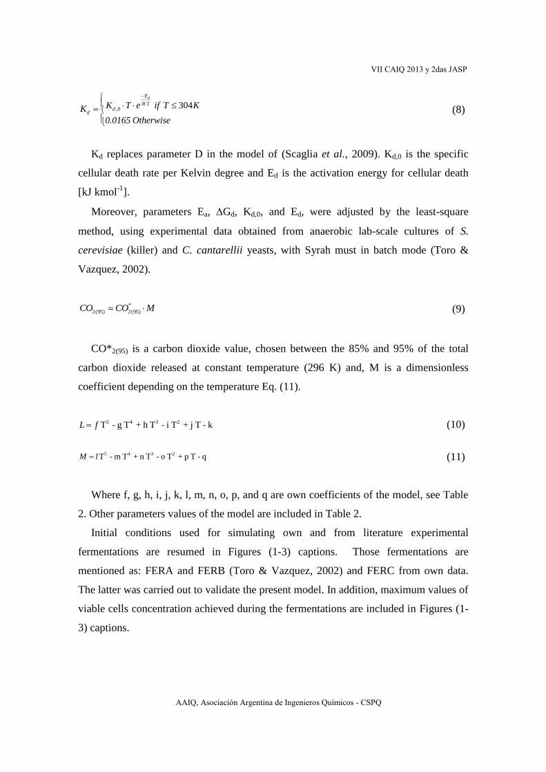
Figure 3, represents the normalized yeasts profile (with respect to its maximum

concentration) attained by simulations and contrasted with the corresponding

experimental profile for the same initial conditions of substrate and yeasts

concentration. Fig. 3 shows for the state variable X, up to 20 hours average in retard,

with respect to experimental X. A preliminary analysis can be that the proposed model

must be improved in reference to estimation of state variables CO2 and X, in case of

their particular values. On variable S, due to the only available data are their final values

in different fermentations, the analysis is considered with the errors defined Eqs. (12

and 13).



0 50 100 150 200 250 300 350 400 450 5000

0.1

0.2

0.3

0.4

0.5

0.6

0.7

0.8

0.9

1

Time [h]

X [N

orm

alis

ed y

east

s co

ncen

trat

ion]

Modelled X

Experimental X

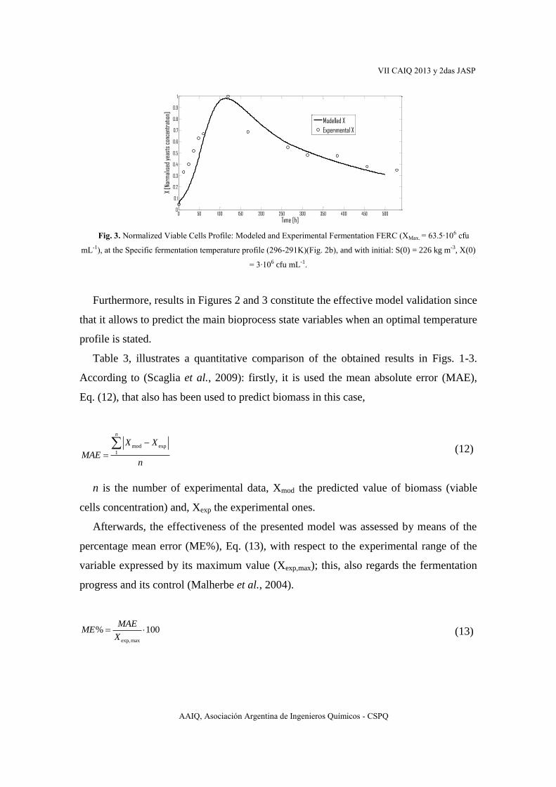
Fig. 3. Normalized Viable Cells Profile: Modeled and Experimental Fermentation FERC (XMax. = 63.5∙106 cfu

mL-1), at the Specific fermentation temperature profile (296-291K)(Fig. 2b), and with initial: S(0) = 226 kg m-3, X(0)

= 3∙106 cfu mL-1.

Furthermore, results in Figures 2 and 3 constitute the effective model validation since

that it allows to predict the main bioprocess state variables when an optimal temperature

profile is stated.

Table 3, illustrates a quantitative comparison of the obtained results in Figs. 1-3.

According to (Scaglia et al., 2009): firstly, it is used the mean absolute error (MAE),

Eq. (12), that also has been used to predict biomass in this case,

mod exp

1

n

X X

MAEn

(12)

n is the number of experimental data, Xmod the predicted value of biomass (viable

cells concentration) and, Xexp the experimental ones.

Afterwards, the effectiveness of the presented model was assessed by means of the

percentage mean error (ME%), Eq. (13), with respect to the experimental range of the

variable expressed by its maximum value (Xexp,max); this, also regards the fermentation

progress and its control (Malherbe et al., 2004).

exp,max

% 100MAE

MEX

(13)



Lastly, in Table 3, it is exposed that both errors are around a typical maximum limit

in biotechnology and process engineering of 10% with respect to data range of variable

biomass, which is compensated with a similar error in the experimental measurement.

Table 3. Comparison between simulated and experimental results.

Fermentation Variable MAE [kg/m3] ME%

FERC X 0.50 7.93

Pfinal

Sfinal

CO2,final

-

-

-

1.2 *

6.8 *

2.8 *

CO2 9.41 7.09

FERA X 0.38 4.14

Pfinal

Sfinal

CO2,final

-

-

-

1.6 *

1.8 *

2.1 *

CO2 3.182 2.93

FERB X 0.38 3.47

Pfinal

Sfinal

CO2,final

-

-

-

2.7 *

9.50

3.4 *

CO2 5.30 5.30

Fundamentally and in general, the predicted profiles do not show appreciable time

retards with respect to the experimental data and achieves an enhanced precision by

estimating four variables compared to own (Ortiz et al., 2006), and other first-

principles models like the ones of (Coleman et al., 2007), and (Phisalaphong et al.,

2006), respectively. This fact was attained with an additional critical variable as the

temperature and the new parameters in the proposed model. Hence, it would be possible

to apply it: in control algorithms to track desired fermentation trajectories with

closeness, and without significant delays in the control actions, or in optimization

strategies to improve the process. Such characteristic is particularly essential during

winemaking process, since a delayed control action on variables, such as temperature or

pH, can generate a sluggish or stuck fermentation or the degradation in organoleptic

properties of wine.



In addition, the model can be used at industrial scale with some adaptation, given

that, other non-isothermal models developed from lab-scale alcoholic fermentations

have been validated or tested with good performance, or highlighted their possible

adaptation, taking into account scale-up effects (Phisalaphong et al., 2006, Colombié et

al., 2007, Malherbe et al., 2004, Coleman et al., 2007). In the work of (Zenteno et al.,

2010), the model was validated for a 10 m3 industrial tank.

5. CONCLUSIONS

In this work, a model for non-isothermal winemaking fermentations, based first-

principles, for predicting the four main bioprocess state variables with enough rigors, is

presented. Since the bioprocess is strongly affected by temperature in aroma and flavor

production, the final wine quality depends on monitoring and controlling on this

variable. Therefore, the model obtained consist of mass balances, predicting state

variables (viable cells, substrate and ethanol concentrations, and CO2 released), coupled

with an energy balance of the system. The latter is done by means of cellular growth

and death parameters, and the CO2(95), all of them in function of temperature in an

interval from 10 to 40°C.

The carried out model has been suitably validated via simulation with published and

own experimental data, showing a proper behavior to predict cellular growth and death

kinetics, ethanol and substrate concentrations, and the CO2 released, at constant

temperature and variable predefined temperature profiles. This allows disposing of a

reliable model to: approximate state variables trajectories and propose advanced control

and optimization strategies.

The model validation reaches to lab-scale winemaking fermentations. It is possible to

use it at industrial scale, in that case, it may be necessary include some aspects not

considered such as: mixing of the fermentation mass and spatial concentration gradients,

heat transfer, etc.

In addition, other topics will be included in next contributions, such as: to track other

variables of the bioprocess as, density and/or pH; to improve parameter estimation with

artificial intelligence tools, etc.



Acknowledgments

We gratefully acknowledge the Universidad Nacional de San Juan and the National

Council of Scientific and Technological Research (CONICET), Argentina, by the

financial support to carry out this work.

References

Aballay, P. M., Vallejo, M. D., Ortiz, O. A. (2006). Temperature control system for high quality wines using a hybrid

model and a neural control system. In Proceedings of the XVI Congresso Brasileiro de Engenharia Química-

COBEQ 2006, Santos, Brazil, 1153-2429.

Aballay, P. M., Scaglia, G. J. E., Vallejo, M. D., Ortiz, O. A. (2008). Non isothermal phenomenological model of an

enological fermentation: modelling and performance analysis. In Proceedings of the 10th International Chemical

and Biological Engineering Conference - CHEMPOR Braga, Portugal.

Aballay, P. M., Scaglia, G. J. E., Vallejo, M. D., Rodríguez, L. A., Ortiz, O. A. (2010). Non-isothermal model of the

yeasts growth in alcoholic fermentations for high quality wines. In Proceedings of the 7th International

Mediterranean & Latin American Modelling Multiconference-I3M2010 y The 4th International Conference on

Integrated Modeling & analysis in Applied Control & Automation IMAACA 2010. Fes, Marruecos, 143-151.

Aballay, P. M., Vallejo, M. D., Scaglia, G. J. E., Serrano, M. E., Rómoli, S., Ortiz, O. A. (2012). Phenomenological

Modelling for Non-Isothermal Wine Fermentation. V Encuentro Regional y el XXVI Congreso Interamericano de

Ingeniería Química – AIQU CIIQ 2012. Montevideo, Uruguay, 32.

Coleman, M. C., Fish, R., Block, D. E. (2007). Temperature-dependent kinetic model for nitrogen-limited wine

fermentations. Applied and Environmental Microbiology, 73, 5875–5884.

Colombié, S., Malherbe, S., Sablayrolles, J. M. (2007). Modeling of heat transfer in tanks during wine-making

fermentation. Food Control, 18, 953–960.

Fischer, U. (2007). Flavours and Fragrances, Chemistry, Bioprocessing and Sustainability. Berlin-Heidelberg:

Springer.

Fleet, G. H., Heard, G. M. (1993). Yeasts: growth during fermentation. Harwood Academic Publishers. Chur,

Switzerland.

Henson, M. A. (2003). Dynamic modeling and control of yeast cell populations in continuous biochemical reactors.

Computers & Chemical Engineering, 27, 1185.

Malherbe, S., Sablayrolles, J. M., Fromion, V., Hilgert, N. (2004). Modeling the Effects of Assimilable Nitrogen and

Temperature on Fermentation Kinetics in Enological Conditions. Biotechnology and Bioengineering, 86, 261-272.

MatlabTM (2008). Version 7.6.0.324 (Release 2008A). The MathWorks, Inc. USA.

Molina, A. M., Agosin, E., Swiegers, J. H., Varela, C., Pretorius, I. S. (2007). Influence of wine fermentation

temperature on the synthesis of yeast-derived volatile aroma compounds. Applied Microbiology and

Biotechnology, 77, 675-687.

Morari, M., Zafiriou, E. (1990). Robust process control. Prentice-Hall International.

Ortiz, O. A., Aballay, P. M., Vallejo, M. D. (2006). Modelling of the killer yeasts growth in an enological

fermentation by means of a hybrid model. In Proceedings of the XXII Interamerican Congress of Chemical

Engineering and V Argentinian Congress of Chemical Engineering. Buenos Aires, Argentina, 451-452.



Ortiz, O. A., Scaglia, G. J. E., Mengual, C. A., Aballay, P. M., Vallejo, M. D. (2009). Advanced Temperature

Tracking Control for High Quality Wines Using a Phenomenological Model. In: de Brito Alves, R.M., Oller do

Nascimento, C.A., and Chalbaud Biscaia Jr., E., eds. 10th International Symposium on Process Systems

Engineering - PSE2009, 27, Part A, Computer Aided Chemical Engineering - Series. Amsterdam (The

Netherlands): Elsevier B.V., 1389-1394.

Phisalaphong, M., Srirattana, N., Tanthapanichakoon, W. (2006). Mathematical modeling to investigate temperature

effect on kinetic parameters of ethanol fermentation. Biochemical Engineering Journal, 28, 36-43.

Sablayrolles, J. M. (2009). Control of alcoholic fermentation in winemaking: Current situation and prospect. Food

Research International, 42, 418-424.

Scaglia, G. J. E., Aballay, P. M., Mengual, C. A., Vallejo, M. D., Ortiz, O. A. (2009). Improved phenomenological

model for an isothermal winemaking fermentation. Food Control, 20, 887-895.

Torija, M. J., Rozès, N., Poblet, M., Guillamón, J. M., Mas, A. (2003). Effects of fermentation temperature on the

strain population of Saccharomyces cerevisiae. International Journal of Food Microbiology, 80, 47-53.

Toro, M. E., Vazquez, F. (2002). Fermentation behaviour of controlled mixed and sequential cultures of Candida

cantarellii and Saccharomyces cerevisiae wine yeasts. World Journal of Microbiology and Biotechnology, 18,

347-354.

Vallejo, M. D., Aballay, P. M., Toro, M. E., Vazquez, F., Suarez, G. I., Ortiz, O. A. (2005). Hybrid Modeling and

Neural Prediction of the Wild Killer Yeast Fermentation Performance in a Winemaking Process. In Proceedings of

the 2nd Mercosur Congress on Chemical Engineering and 4th Mercosur Congress on Process Systems

Engineering. Rio de Janeiro, Brazil, 1-10.

Zenteno, M. I., Pérez-Correa, J. R., Gelmi, C. A., Agosin, E. (2010). Modeling temperature gradients in wine

fermentation tanks. Journal of Food Engineering, 99, 40-48.

validation of a phenomenological model for the state ... · validation of a phenomenological model...

Documents