validating the capm and the fama-french three-factor · pdf filethe latter limitation,...

Validating the CAPM and the Fama-French

three-factor model

Michael Michaelides

Department of Economics,

Virginia Tech, USA

Aris Spanos

Department of Economics,

Virginia Tech, USA

January 2016

Abstract

The primary aim of this paper is to revisit the empirical adequacy of the

structural CAPM and the Fama-French three-factor model. By distinguishing

between the structural and statistical models, where the latter comprises the

probabilistic assumptions imposed on the data, the paper shows that these

structural models are statistically misspecified. This raises questions about the

Fama-French three-factor model which was justified in terms of the significance

of the added factors. If the original CAPM is statistically misspecified, however,

the significance of the added factors is questionable because it is likely that the

nominal error probabilities used by these tests are very different from the actual

ones. The paper respecifies the statistical models underlying the CAPM and

Fama-French three-factor structural models. The respecification results in a

Student’s t VAR(1) and Dynamic Linear Regression models which provide a

sound basis for revisiting the empirical adequacy of the structural models. The

statistical inference results, based on the Fama-French data, call into question

the empirical adequacy of these models.

1

1 IntroductionAsset pricing theory is concerned with the analysis of prices or values of claims on

financial assets in a world of uncertainty. Evaluation of financial asset riskiness and

associated premium is one of the most fundamental issues faced by individual investors

and financial institutions for both pricing and investing in such assets. How does

the risk of an investment affects, or should affect, its expected return? Why do

some financial assets tend to pay higher average returns than others? How are the

various types of risk measured? Asset pricing theory is concerned with providing

answers to these questions and continues to be one of the most important theoretical

underpinning of portfolio management and investment analysis.

The early work of Markowitz (1952) marked a new era in asset pricing theory. In

his pioneering paper, Markowitz argued that a risk averse investor who focuses on

the mean and variance of the returns of individual assets contained in a portfolio, is

motivated by the highest possible profit given the lowest possible risk. By providing

a mathematical justification, he showed that an investor wants to maximize the mean

and minimize the variance, and therefore, the optimal portfolio is one whose mean-

variance combination is in the efficient frontier. Yet, it was Tobin’s (1958) separation

theorem that extended the logic of efficient frontier using one’s attitude towards risk.

He demonstrated that an investor who already holds the optimal combination of risky

assets and is able to borrow or lend at the risk free rate, can decide whether to borrow

or lend, depending on his attitude towards risk. His main conclusion was that the

single market portfolio is the efficient frontier that dominates any other combination.

Although the groundwork of Markowitz and Tobin was simple and intuitive, it

presented difficulties in the computation of the variance-covariance matrix when the

number of assets was very large. The latter limitation, together with the absence of

a theory for estimating the correct cost of capital of an investment in the influential

work of Modigliani and Miller (1958), provided the primary motivation for Treynor

(1962, published 1999), Sharpe (1964), Lintner (1965a, 1965b) and Mossin (1966), to

independently introduce the most popular model in the asset pricing literature; the

Capital Asset Pricing Model (CAPM).

The theoretical CAPM has the following form:

(−)=(−) =1 (1)

where, is the expected return of asset , is the expected return of the risk free

asset, (−) is the expected excess asset return (risk premium) of asset is thebeta coefficient of asset , is the expected return of the market, and (−) isthe expected excess market return (market premium).

The model relates − and − via , which is a standardized measure ofsystematic risk - not the total risk - based upon an asset’s covariance with the mar-

ket portfolio. The theoretical underpinnings of the CAPM depended on a number

of strong assumptions. First, investors are rational and risk averse, they all share

homogeneous expectations, and behave in a manner as to maximize their economic

2

utility. Second, they are broadly diversified across a range of assets and can bor-

row/lend unlimited amounts under the risk free rate of interest. Third, the stock

market functions under conditions of perfect competition and equilibrium. Investors,

- who all have access to available information - have the right to buy or/and sell any

amount of shares, at any period of time, having a very little impact, if any, on the

market price. Fourth, investors are not burdened of any transaction costs and at

the same time taxation and any other sort of restrictions are similarly absent. Fifth,

returns are Normally distributed, with known means, variances and covariances.

For inference purposes the CAPM is usually embedded into a statistical model of

the form:

(−)= + (−) + =1 =1 (2)

where, is the returns of asset , is the returns of a risk free asset, is

the intercept (Jensen’s alpha), is the beta coefficient and is the returns of

the market. The error term, , is assumed to satisfy the following probabilistic

assumptions:

(i) ()=0 (ii) ()=2−22 (iii) ( −)=0

(iv) ( )6=0 for 6= =1 (v) ( )=0 for 6= =1 (3)

Despite its simplicity, the CAPM is hampered by its very strong set of assump-

tions. The fact that every assumption is likely to be violated in the real world,

motivated academics and professionals to extend the CAPM, in an attempt to im-

prove it by relaxing some of the assumptions. Some of the well-known extensions to

the model include, the Black (1972) CAPM, the Intertemporal CAPM (ICAPM) by

Merton (1973), and the Consumption CAPM (CCAPM) by Breeden (1979). Further,

subsequent work by Ross (1976), Chen et al. (1986), Fama and French (1992, 1993),

Carhart (1997), among others, has introduced several sources of risk - called factors -

that determine returns besides the original market beta. The extended CAPM takes

the generic form:

−=+1(−)+P

=2 + =1 =1 (4)

Did the CAPM developed into a better pricing model since its introduction? From

the theory perspective, the extensions of CAPM provide a clearer, more refined, and

theoretically a more appealing framework which attempts to bridge the gap between

theory and data in more elaborated ways.

The bridging of the gap between theory and data, however, has a weak link. The

validity of the probabilistic assumptions (directly or indirectly) imposed on the data

is not thoroughly tested. As a result, the various improvements of the original CAPM

have not been subjected to adequate empirical scrutiny. The inclusion of additional

factors provides sound empirical improvements to the original structural model only

when they are statistically justified. The latter requires that the estimated model

3

in the context of which the additional factors are tested is statistically adequate: its

probabilistic assumptions are valid for the data in question.

The primary objective of this paper is to revisit the CAPM and the Fama-French

extension with a view to evaluate their empirical validity vis-a-vis the data by thor-

oughly testing the probabilistic assumptions (implicitly) imposed on the data. It is

shown that both the original CAPM and the Fama-French three-factor models are

empirically invalidated using the Fama and French (1993) data.

2 Statistical vs. Substantive modelsThe current situation where a modeler attempts to improve the scope of a theoretical

(structural) model by adding potentially relevant variables has a serious flaw. The

reliability of the significance test for the coefficients of such variables depends crucially

on whether the original model is statistically adequate. When that is not the case,

the tests of significance are likely to be unreliable because of sizeable discrepancies

between their nominal and actual error probabilities. This serious flaw stems from

not distinguishing between a theoretical (structural) model and a statistical model;

see Spanos and McGuirk (2001), Spanos (2009).

A structural model is a mathematical formulation of a theory that aims to ap-

proximate a real-world phenomenon of interest with a view to provide an adequate

explanation. Justifiably, such models could be described as simplifications of the

real world because they typically rely on strong assumptions. Moreover, by replacing

some of the unrealistic assumptions with more realistic ones the theory’s fecundity

can be enhanced. On the other hand, a statistical model represents the probabilistic

assumptions imposed (directly or indirectly) on the data. Its role is to ensure the

error-reliability of all statistical inferences based on the estimated model since the in-

ference procedures invoke these assumptions. In practice, these assumptions are not

clearly brought out because they are imposed on the data indirectly via the structural

model in conjunction with the error term assumptions, such as (3), and not the ob-

servable random variables involved. Hence, the statistical premises are rarely tested

thoroughly, and as a result the endeavors to enhance the substantive adequacy of

the estimated structural model are often of questionable value on empirical grounds.

To avoid this conundrum one needs to establish the adequacy of the implicit statis-

tical model before probing for the appropriateness of substantive refinements of the

original structural model.

In the asset pricing literature, more often than not, statistical adequacy is not

properly secured. As a result, this often undermines the credibility of inferences

relating to the inclusion of additional potentially relevant variables. Indeed, no trust-

worthy evidence for or against the substantive theory can be secured when the implicit

statistical model is misspecified.

In order to avoid unreliable inference results, one needs to test the validity of the

probabilistic assumptions imposed on the particular data, or more precisely, on the

stochastic process underlying the data. In the case of the statistical CAPM and its

4

extensions, the statistical Generating Mechanism (GM) used in the literature is:

= + β>X + =1 2 ∈N:=(1 2 )

where B>:=(>1 >2

>) and X:=(12 ) Hence, the probabilistic as-

sumptions imposed on the underlying observable process are given in table 1.

Table 1 - Multivariate Normal/Linear Regression (LR) Model

Statistical GM: y=α+B>X+u ∈N

[1] Normality (y|X=x)∼N( )[2] Linearity (y|X=x)=α+B

>X

[3] Homoskedasticity (y|X=x)=V

[4] Independence (y|X=x) independent process,[5] t-invariance: (αBV) are constant over

α=(μ1−B>μ2)∈R B= (Σ−122Σ21)∈R V=(Σ11−Σ>21Σ

−122Σ21)∈R+

μ1=(y) μ2=(X) Σ11= (y) Σ12=(yX) Σ22=(X)

The conversion of the CAPM into a model which is estimable with the given data,

implicitly involves the specification of the statistical model. In practice, one needs to

make the implicit probabilistic assumptions concerning explicit in order to specify the

statistical model; the inductive premises of interest. Estimating the structural model

directly leaves no room for testing the validity of either the implicit statistical premises

or the theory information vis-a-vis the data in question. Estimating the structural

model directly does not allow one to delineate between two different sources of error,

the substantive and statistical inadequacy, and apportion blame.

To address this problem one needs to separate the substantive and the statistical

information ab initio. This will enable one to delineate and probe for different poten-

tial errors at different stages of modeling. The question that needs to be answered

is: where does the statistical model come from if not from the structural model?

The answer is that from a purely probabilistic perspective a statistical model can be

viewed as a parameterization of the observable stochastic process (Spanos, 2006a):

Z:=(X) =1 2 ∈N (5)

giving rise to the observed data. In the case of the CAPM, there are three data series

() and one needs to view them as separate entities whose probabilistic

structure gives rise to the parameterization of the statistical model in table 1. Hence,

from this perspective, the relevant statistical model is :

= + 11 + 22 + =1 2 ∈N (6)

where = 1= and 2= The CAPM is a special case of this statistical

model in the sense that the nesting restrictions take the form:

=0 1+2=1 =1 2 (7)

5

Unfortunately, the literature has focused exclusively on the zero constant, and ignored

the adding up restrictions.

In general, the structural and statistical models are related via their respective

parameters in the form of an implicit form:G(αθ)=0 (8)

The structural parameters α are said to be identified there exists a unique solution

of (8) for α in terms of θ; see Spanos (1990). In practice, there are more statistical

than structural parameters and probing for substantive adequacy requires one to test

the over-identifying restrictions.

2.1 The Fama-French three-factor modelThe inability of the static CAPM to explain the cross-section data of average returns,

triggered the interest of Fama and French (1992) to bring together earlier empirical

work and to propose an alternative model that includes additional variables. Based on

the relationships between a number of variables and returns, Fama and French (1992)

used cross-sectional regressions to compare the explanatory power of these variables.

Such variables included the size effect, documented by Banz (1981), the positive

relation between book-to-market equity (BE/ME) and average return, supported by

Rosenberg et al. (1985), as well as the association between earnings-price ratios

(E/P) and leverage with average returns - in tests that also include size and market

beta -, proposed by Basu (1983) and Bhandari (1988) respectively. As a result, they

concluded that the explanatory power of the E/P and leverage variables vanishes when

size and BE/ME variables are included in the regressions and furthermore, that the

CAPM itself cannot fully explain the cross-section of asset returns. Supplementary,

Fama and French (1993) extended on their findings by including the size and BE/ME

variables - besides the market beta - to the original CAPM and used time-series

regressions to further test the explanatory power of these variables. This development

gave rise to the famous three-factor model.

The statistical formulation of the Fama and French (1993) three-factor model is:

(−)=+1(−)| z CAPM

+2+3+ =1 2 ∈N(9)

where, accounts for the spread in returns between ‘small’ and ‘big’ firms, based

on the market capitalization, and accounts for the spread in returns between

‘value’ and ‘growth’ stocks based on the BE/ME ratios.

Over time, the work of Fama and French (1992, 1993) has been criticized from

various perspectives. One key criticism concerns the absence of a theory to justify

the constructed portfolios the Fama-French models employ. Using portfolios of assets

is viewed as a way to reduce the errors in the assessment of the estimated parameters

(see Blume, 1970), but critics claim that there is no convincing theory to determine

what constitutes a ‘small’/‘big’ stock or a ‘high’/‘medium’/‘low’ stock. In addition,

many argue that the Fama-French models are purely empirically motivated. Further,

Black (1993a, 1993b) mentioned that their results are affected by data mining bias,

6

while others, among them Kothari et al. (1995) and Banz and Breen (1986) suggested

the existence of survivorship bias. In addition, Kothari et al. (1995), argued that

the betas estimated with monthly returns are different when compared with betas

estimated with annual returns. Despite such criticisms, the ready access to the Fama-

French portfolios made the proposed framing very popular in the recent empirical

literature on asset pricing.

Unfortunately, very little attention has been paid by this literature to the validity

of the implicit statistical premises for either the CAPM or the Fama-French models.

As a result, the Fama-French approach to the omitted variable problem conflates

statistical with substantive misspecification and the accumulated empirical evidence

need to be revisited with a view to assess their trustworthiness.

2.2 Revisiting the CAPMand Fama-French three-factor modelThe aim of this study is to test the validity of the statistical premises invoked by the

original CAPM and the extended Fama-French three-factor model, using the data

originally used by Fama and French (1993). The data set spans a 342 month period

from July 1963 to December 1991. All data are downloaded from French’s online

data library where the reader can find additional clarifying details and information.

(a) The dependent variables are the monthly returns for 25 stock portfolios formed

in terms of size and BE/ME.

Table 2 - Dependent Variables

Size\BE/ME Low 2 3 4 High

Small 2 3 4

2 2 22 23 24 2

3 3 32 33 34 3

4 4 42 43 44 4

Big 2 3 4

(b) The explanatory variables are the factors included in the CAPM and the

three-factor model specifications.

Table 3 - Explanatory Variables

− Excess market return

Market return

Size factor (Small Minus Big)

Value factor (High Minus Low)

Risk free rate

Moreover, the following additional variables are used with a view to capture the

statistical regularities exhibited by the data.

(i) Discrete Gram-Schmidt orthonormal trend polynomials:

()=[()k()k] =0 1 2 (10)

7

where 0() 1() 2() () is the orthogonal basis of 0 2 for0=(1 1 1) =(1 2 )

These (discrete) orthogonal polynomials are used to ‘capture’ any mean or vari-

ance heterogeneity in the data. Extending ordinary polynomials to orders higher than

3 gives rise to serious collinearity problems.

(ii) Monthly seasonal dummy variables, =1 2 12 =1 2 are used

to capture any seasonal mean heterogeneity in the data.

⎧⎪⎪⎪⎨⎪⎪⎪⎩1 if =January

2 if =February...

...

12 if =December

, =

½1 if =

0 if 6= ∀=1 2 12 (11)

where, =P

=1 is the deterministic seasonality.

(iii) Lags in both dependent and explanatory variables to capture any temporal

dependence in the data.

3 Testing for statistical adequacyThe adequacy of a statistical model is assessed by thoroughly testing its probabilistic

assumptions. In the case of the CAPM, the implicit statistical model is the Multi-

variate Normal LR model in table 1 which is defined in terms of assumptions [1]-[5].

The statistical model in table 1 can be viewed as a parameterization of a Normal,

Independent and Identically Distributed (NIID) process Z ∈N underlying dataZ0. Formally, the probabilistic reduction takes the form:

(Z1Z2 Z;φ)IID=

Q=1

(Z;ϕ)=Q=1

(y|X;ϕ1)(X;ϕ2) (12)

where the distribution underlying the statistical model M(z) is (y|X;ϕ1) with

ϕ1:=(β0B>1 Σ) the associated parameterization; the specification ofM(z) in terms

of a complete, internally consistent and testable list of assumptions [1]-[5]; see Spanos

(1986).

The first stage of probing for statistical adequacy is to relate various plots of the

original data to model assumptions. In this case one can informally assess the appro-

priateness of the model assumptions by assessing the validity of the NIID reduction

assumptions given below.

Table 4: Reduction vs. model assumptions

Reduction: Z ∈N Model: (y|X=x) ∈NN −→ [1]-[3]

I −→ [4]

ID −→ [5]

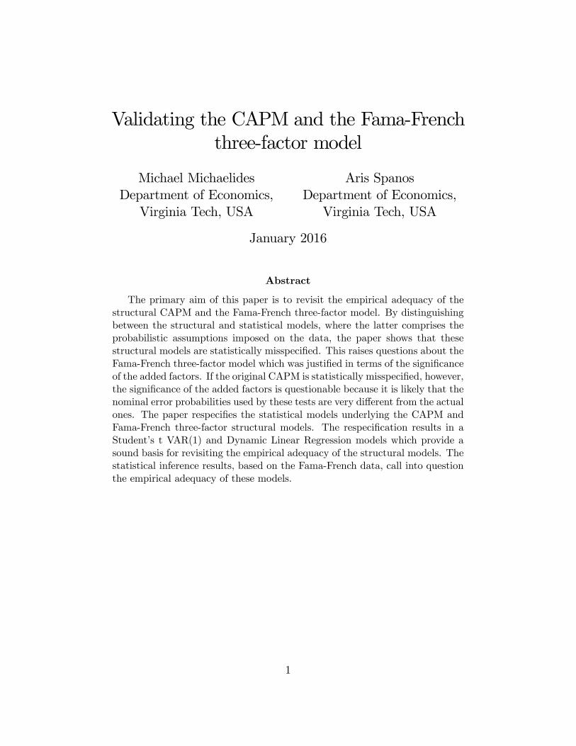
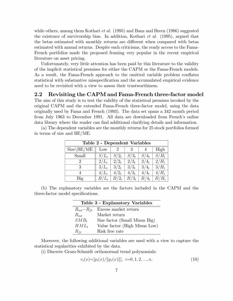
The t-plots of the three data series indicate that the IID assumptions are likely

to be invalid because one can detect both trends (heterogeneity) and irregular cycles

8

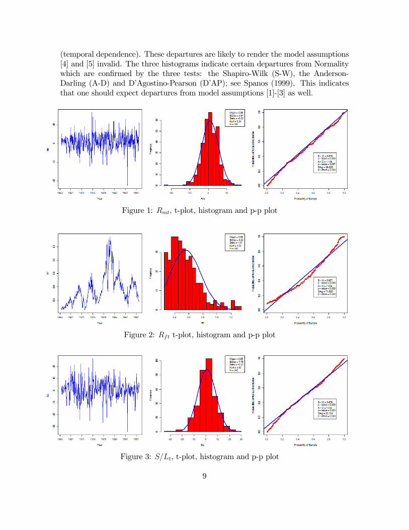
(temporal dependence). These departures are likely to render the model assumptions

[4] and [5] invalid. The three histograms indicate certain departures from Normality

which are confirmed by the three tests: the Shapiro-Wilk (S-W), the Anderson-

Darling (A-D) and D’Agostino-Pearson (D’AP); see Spanos (1999). This indicates

that one should expect departures from model assumptions [1]-[3] as well.

Figure 1: , t-plot, histogram and p-p plot

Figure 2: t-plot, histogram and p-p plot

Figure 3: , t-plot, histogram and p-p plot

9

3.1 Mis-Specification (M-S) TestingCaution is advisable in taking the above M-S tests for Normality at face value be-

cause the tests invoke IID assumptions which are questionable in this case. Hence,

in practice it is a better strategy to begin with M-S testing with the other model

assumptions since departures from assumptions [2]-[5] call the results of Normality

tests into question.

The M-S testing of model assumptions [2]-[5] will be based on the following aux-

iliary regressions which aim to provide joint M-S tests for all departures that affect

the regression and skedastic functions, respectively:b=10 + γ>1X +X

=12| z

[51]

+ γ>3 ψ| z [2]

+X

=1γ>4Z−| z [4]

+X−1

=1| z

[52]

+ 1(13)

b2=20 +X

=15| z

[53]

+ γ>6 ψ +X

=1γ>7Z

2−| z

[3]+[4]

+ 2(14)

where, b are the residuals of the statistical formulation in (6), for portfolio , are the terms of the Gram-Schmidt orthonormal polynomial of order =1

Z:=(X), for X:=(1 2 ), ψ:=(·) ≥ =1 2 and are the error terms; see Spanos (2010).

The joint M-S tests employed are -type and are based on assessing the signif-

icance of the additional terms that represent generic departures form assumptions

[2]-[5] (table 5).

Table 5 - M-S testing hypotheses

[2] Linearity 0: γ3=0 vs 1: γ3 6=0

[3] Homo/city

½static

dynamic

0: γ6=0 vs 1: γ6 6=00: γ7=0 vs 1: γ7 6=0 =1

[4] Independence 0: γ4=0 vs 1: γ4 6=0 =1 [5] t-invariance:

[5.1] mean homogeneity 0: 2=0 vs 1: 2 6=0 =1 [5.2] seasonality 0: =0 vs 1: 6=0 =1 − 1[5.3] variance homogeneity 0: 5=0 vs 1: 5 6=0 =1

Table 6 - M-S results for the CAPM

22 33 44

[2] 1522[220] 2188[114] 2749[066] 3269[007] 3713[012]

[3] 4929[001] 8844[000] 8526[000] 7554[000] 6992[000]

[4] 8002[000] 4662[003] 2443[064] 1719[084] 1355[257]

[5.1] 4481[001] 3039[007] 3348[068] 3442[065] 0114[736]

[5.2] 3531[000] 3278[000] 1683[076] 1404[170] 2018[026]

[5.3] 8773[003] 5680[018] 7401[007] 14272[000] 4547[011]

10

The M-S testing results for five selected portfolios of the CAPM (table 6) suggest

that, the homoskedasticity [3], independence [4], and the t-invariance [5] assumptions

are often invalid. In fact, at least two of these assumptions are not satisfied for each

portfolio (see table B1-Appendix). Departures from the linearity assumption [2] are

not as clear, especially in light of the fact that for a large sample size, one has to

choose much smaller thresholds for significance when using the p-values; see Lehmann

(1986). With =342 a threshold of =01 is more appropriate.

The M-S results of the Fama-French three-factor model in table 7, indicate similar

departures from the statistical model assumptions. There are some differences like

the statistically significant improvements of the t-invariance assumption (see table

B2-Appendix), but they are not substantive enough to assure one that these models

improve the statistical adequacy of the original CAPM. Indeed, certain M-S tests

results, like linearity, appear to suggest worsening of the CAPM statistical inadequacy.

Table 7 - M-S results for Fama-French three-factor model

22 33 44

[2] 5058[000] 1557[186] 1114[350] 7157[000] 2415[009]

[3] 3482[001] 4772[000] 2748[006] 3108[002] 8273[000]

[4] 4130[001] 0985[427] 1232[270] 2137[008] 2017[076]

[5.1] 2426[048] 2029[074] 0417[519] 0370[544] 0400[527]

[5.2] 2973[001] 1031[419] 2160[016] 13191[000] 1180[300]

[5.3] 1514[185] 2234[051] 7652[006] 3788[052] 4381[005]

Although, in light of the M-S testing results in table 6, one needs to exercise caution

in interpreting the results for the Normality assumption [1], clear departures are

indicated for both families of models. For the sake of argument, only 2 of 25 portfolios

fail to reject normality in the case of CAPM (see table A1 - Appendix).

Table 8 - M-S testing for Normality

22 33 44

[1.1] 0991[026] 0974[000] 0973[000] 0976[000] 0970[000]

[1.2] 1088[007] 1791[000] 1886[000] 1753[000] 1301[002]

[1.3] 8999[011] 33953[000] 23956[000] 29688[000] 25767[000]

[1.1] 0991[037] 0985[002] 0992[050] 0985[001] 0983[000]

[1.2] 0413[336] 0694[069] 0395[371] 0722[059] 1323[002]

[1.3] 13536[001] 21517[000] 10842[004] 14233[001] 14580[001]

In summary, the joint M-S testing using auxiliary regressions indicate clearly that

the Multivariate Normal LR model suffers from serious statistical misspecifications.

The residuals indicate major departures from the all the statistical assumptions and

the only assumption which seems to hold is Linearity. Taken together, the above M-S

testing results call into question the empirical credibility of the Fama-French exten-

sion of the CAPM because their substantive adequacy was based on a statistically

11

misspecified model. Before the Fama-French three-factor model can be substantively

assessed in an empirically reliable way, one needs to respecify the implicit statistical

model associated with the CAPM with a view to account for the chance regularities

in the data that are not accounted for by the original model.

3.2 Respecification: Normal VAR(1)In light of the act that the Normality plays a crucial role in the original Markowitz

(1952) optimal portfolio theory as well as the CAPM and its extensions, an attempt

will be made to account for all the other departures indicated by the above M-S

testing results without changing Normality.

Table 9 - Normal Vector Autoregressive [VAR(1)] model

Statistical GM: Z=α0+

X=1

γ+

−1X=1

δ+A>1 Z−1+u ∈N

[1] Normality (Z|Z0−1;θ) Z0−1:=(Z−1 Z1) is Normal,

[2] Linearity (Z|(Z0−1))=α0+X=1

γ+

−1X=1

δ+A>1 Z−1

[3] Homosk/city (Z|(Z0−1))=Ω is free of Z0−1

[4] Markov Z ∈N is a Markov process,

[5] t-invariance: θ:=

½(i) coefficients (α0A1)

(ii) covariance (Ω)

α0 = μ−A>1 μ A1 = Σ−10 Σ1 Ω = Σ0−Σ>

1Σ−10 Σ1

The respecification takes the form of replacing the original reduction assumptions im-

plicitly imposed on the observable stochastic process Z:=(X) =1 2 ∈Nwith more appropriate ones. Departures from assumptions [4] and [5] suggest that the

IID assumptions are clearly invalid and need to be replaced with more appropriate

assumptions that allow for temporal dependence and certain forms of heterogeneity.

The generic way to do that is to use lags, trends and seasonal dummy variables. For-

mally, assuming that Z:=(X) =1 2 ∈N is Normal, Markov (M) andmean heterogeneous but covariance stationary (S) gives rise to the Normal VAR(1)

heterogeneous model given in table 9. The probabilistic reduction takes the form:

(Z1Z2 Z;φ(t))= (Z1;ψ1)

Q

=2(Z|Z−1;ψ(t)) == (Z1;ψ1)

Q

=2(Z|Z−1;ψ(t))(15)

where ψ(t) includes both the Gram-Schmidt trend polynomials and seasonal dum-

mies. Note that making the further reduction:

Q=2

(Z|Z−1;ψ(t)) =Q=2

(|XZ−1;ψ1())·(X|Z−1;ψ2()) (16)

12

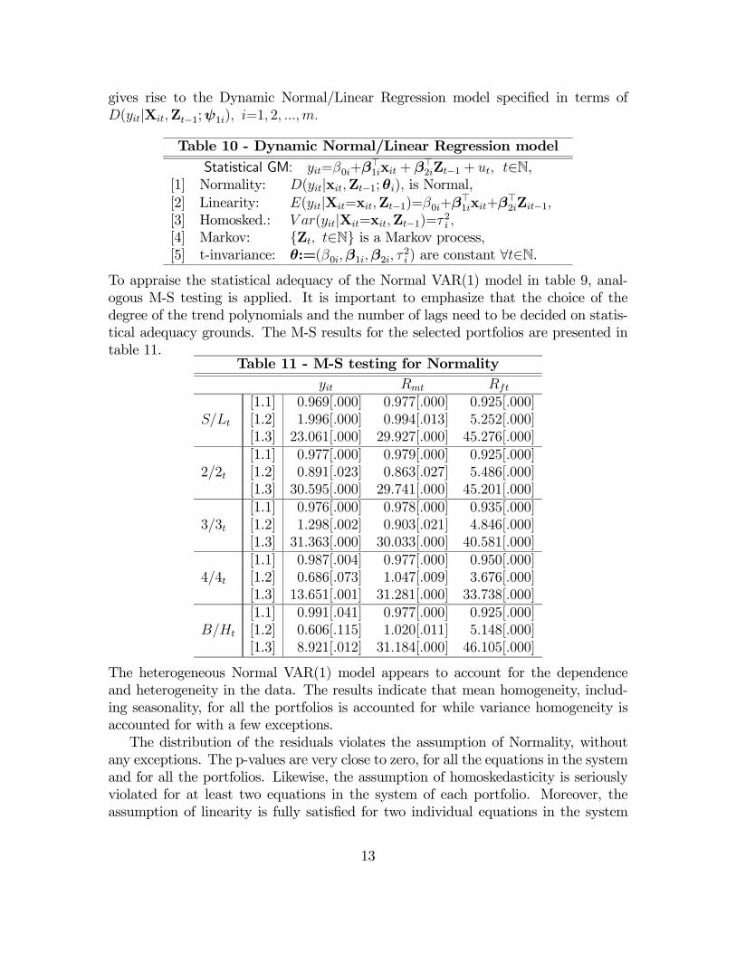
gives rise to the Dynamic Normal/Linear Regression model specified in terms of

(|XZ−1;ψ1) =1 2

Table 10 - Dynamic Normal/Linear Regression model

Statistical GM: =0+β>1x + β

>2Z−1 + ∈N,

[1] Normality: (|xZ−1;θ) is Normal,[2] Linearity: (|X=xZ−1)=0+β

>1x+β

>2Z−1

[3] Homosked.: (|X=xZ−1)= 2 [4] Markov: Z ∈N is a Markov process,[5] t-invariance: θ:=(0β1β2

2 ) are constant ∀∈N.

To appraise the statistical adequacy of the Normal VAR(1) model in table 9, anal-

ogous M-S testing is applied. It is important to emphasize that the choice of the

degree of the trend polynomials and the number of lags need to be decided on statis-

tical adequacy grounds. The M-S results for the selected portfolios are presented in

table 11.Table 11 - M-S testing for Normality

[1.1] 0969[000] 0977[000] 0925[000]

[1.2] 1996[000] 0994[013] 5252[000]

[1.3] 23061[000] 29927[000] 45276[000]

[1.1] 0977[000] 0979[000] 0925[000]

22 [1.2] 0891[023] 0863[027] 5486[000]

[1.3] 30595[000] 29741[000] 45201[000]

[1.1] 0976[000] 0978[000] 0935[000]

33 [1.2] 1298[002] 0903[021] 4846[000]

[1.3] 31363[000] 30033[000] 40581[000]

[1.1] 0987[004] 0977[000] 0950[000]

44 [1.2] 0686[073] 1047[009] 3676[000]

[1.3] 13651[001] 31281[000] 33738[000]

[1.1] 0991[041] 0977[000] 0925[000]

[1.2] 0606[115] 1020[011] 5148[000]

[1.3] 8921[012] 31184[000] 46105[000]

The heterogeneous Normal VAR(1) model appears to account for the dependence

and heterogeneity in the data. The results indicate that mean homogeneity, includ-

ing seasonality, for all the portfolios is accounted for while variance homogeneity is

accounted for with a few exceptions.

The distribution of the residuals violates the assumption of Normality, without

any exceptions. The p-values are very close to zero, for all the equations in the system

and for all the portfolios. Likewise, the assumption of homoskedasticity is seriously

violated for at least two equations in the system of each portfolio. Moreover, the

assumption of linearity is fully satisfied for two individual equations in the system

13

model but often violated for the third equation. A possible explanation for this

violation can be the skewness of the probability distribution of or a symptom of

the existence of dynamic heteroskedasticity in the form of second order dependence.

22

[2] 0616[605] 0082[970] 2932[034] [2] 0410[746] 0325[807] 3527[015]

[3] 3677[001] 2791[001] 17640[000] [3] 2842[010] 3301[000] 17485[000]

[4] 2310[076] 1727[161] 0588[623] [4] 1064[364] 1366[253] 0716[543]

[5.1] 1980[160] 0244[622] 4048[018] [5.1] 1313[253] 1371[243] 2679[022]

[5.2] 0067[999] 0035[999] 0041[999] [5.2] 0012[999] 0021[999] 0054[999]

[5.3] 9363[002] 0671[413] 2471[117] [5.3] 2237[136] 0167[683] 2983[085]

33 44

[2] 0117[950] 0073[974] 6160[000] [2] 0374[772] 0379[768] 8931[000]

[3] 3985[001] 3300[000] 16160[000] [3] 3394[003] 3594[002] 13380[000]

[4] 1506[213] 1291[278] 0738[530] [4] 1580[194] 1228[299] 1667[174]

[5.1] 2455[118] 1313[253] 3067[010] [5.1] 1267[261] 1640[201] 1316[252]

[5.2] 0013[999] 0012[999] 0133[999] [5.2] 0028[999] 0018[999] 0113[999]

[5.3] 2925[088] 0107[744] 2543[112] [5.3] 2492[115] 0037[848] 1780[183]

[2] 0485[693] 0230[875] 3590[014]

[3] 2223[041] 2840[001] 15100[000]

[4] 0867[458] 1008[390] 0747[525]

[5.1] 1980[160] 1667[198] 2339[042]

[5.2] 0023[999] 0016[999] 0072[999]

[5.3] 1920[126] 0001[988] 1585[209]

Although on statistical adequacy grounds the heterogeneous Normal VAR(1) model is

an improvement over the original Multivariate Normal LRmodel, it is not statistically

adequate. However, the M-S testing results provide us with helpful information with

regard to the next stage of respecification.

4 The Student’s t VAR(1)At this stage, the aim is to specify a more appropriate probabilistic structure, com-

pared to the Normal VAR() model, with a view to account for all the departures

indicated by M-S testing results, especially the clear departures from the Normal-

ity and homoskedasticity assumptions. These departures suggest that the best way

forward is to consider another member of the elliptically symmetric family of dis-

tributions since all its members have heteroskedastic conditional variances except

the Normal which is characterized by homoskedasticity within this family; see Fang

et al. (1990). The distribution that suggests itself is the Multivariate Student’s t

distribution; see Spanos (1994).

14

The probabilistic assumptions of the Student’s t VAR(; ) and the Normal VAR()

models differ in one crucial respect: the former has a heteroskedastic conditional vari-

ance; see assumption [3] in table 12.

Table 12 - Student’s t Vector Autoregressive [VAR(1; =4)] model

Statistical GM: Z=α0 +

X=1

γ +

−1X=1

δ +A>1 Z−1+u ∈N

[1] Student’s t (Z|Z0−1; θ) Z0−1:=(Z−1 Z1)

is Student’s t with d.f.

[2] Linearity (Z|(Z0−1))=α0+X=1

γ+

−1X=1

δ+A>1 Z−1

[3] Heteroskedasticity (Z|(Z0−1))=³

+−2

´V¡Z0−1

¢is free of Z0−1

¡Z0−1

¢=nI +V

−1 [Z−1 −μ]>Q−1 [Z−1 −μ]o

[4] Markov Z ∈N is a Markov (1) process,

[5] t-invariance: θ:=

½(i) mean (α0A1μ)

(ii) variance (VQ)

The Student’s t VAR(; ) autoskedastic function is a quadratic function of the con-

ditioning variables in mean deviation from their marginal means which include both

the trend heterogeneity as well as the seasonality terms.

A thorough M-S testing is applied to the heterogeneous Student’s t VAR(1; =4)

model, using joined M-S testing in the form of auxiliary regressions, which are very

similar to the ones used before, with one difference. The residuals are rescaled by a

t-varying conditional variance in order to account for the heteroskedastic conditional

variance. The standardized residuals are defined by:

bu =L−1 (Z−bZ) LL> =

d (Z|σ(Z0−1)) (17)

The Student’s t assumption is tested by adapting the Kolmogorov-Smirnov (K-S)

and the Anderson-Darling (A-D) non-parametric tests. The M-S testing results for

five selected portfolios in table 13 provide good evidence for the Student’s t assump-

tions. Failure to disprove the assumptions in table 12, and especially heteroskedastic-

ity, indicates to support the statistical adequacy of the underlying model; see tables

A2 and B3-B5 (Appendix) for M-S testing results of the rest of the portfolios.

15

Table 13 - M-S testing for Student’s t

[1.1] 0064[063] 0051[171] 0480[000]

[1.2] 4552[005] 1567[161] 127532[000]

[1.1] 0056[117] 0049[197] 0480[000]

22 [1.2] 1698[136] 1506[175] 127525[000]

[1.1] 0038[376] 0049[193] 0478[000]

33 [1.2] 0703[556] 0717[545] 127098[000]

[1.1] 0031[517] 0032[503] 0478[000]

44 [1.2] 0401[847] 0307[933] 127147[000]

[1.1] 0042[306] 0036[415] 0478[000]

[1.2] 1069[323] 0524[723] 126902[000]

22

[2] 0418[741] 0017[997] 1196[311] [2] 0170[916] 0065[978] 1371[252]

[3] 0105[746] 0070[792] 0001[984] [3] 0542[462] 0557[456] 0159[691]

[4] 1950[121] 1745[158] 2137[095] [4] 1810[145] 1639[180] 1611[187]

[5.1] 1455[229] 0413[521] 3650[027] [5.1] 0779[378] 0478[490] 5034[007]

[5.2] 0360[970] 0164[999] 0154[999] [5.2] 0106[999] 0163[999] 0313[983]

[5.3] 6527[011] 0033[855] 0081[776] [5.3] 0951[330] 0026[873] 0287[593]

33 44

[2] 0147[931] 0116[951] 1643[179] [2] 0020[996] 0011[998] 2987[008]

[3] 1824[178] 2832[093] 0021[884] [3] 0664[416] 0131[717] 0202[654]

[4] 2690[046] 2281[079] 2792[041] [4] 1183[316] 0956[414] 3307[021]

[5.1] 0001[999] 1224[269] 2948[087] [5.1] 0174[677] 0722[396] 4361[038]

[5.2] 0352[973] 0222[996] 0406[953] [5.2] 0297[986] 0201[998] 0268[991]

[5.3] 3410[066] 0138[710] 0023[881] [5.3] 6888[009] 0035[851] 0027[871]

[2] 0120[948] 0048[986] 1510[212]

[3] 1887[170] 1108[293] 1170[280]

[4] 2123[097] 1821[143] 1348[259]

[5.1] 0126[723] 0642[424] 0925[337]

[5.2] 0177[999] 0169[999] 1144[999]

[5.3] 9718[002] 0482[488] 1267[261]

The M-S results indicate that the Students’t VAR(1; =4) model is statistically

adequate and it accounts for all the statistical systematic information in the Fama-

French data.

What is particularly important to emphasize is that to be able to account for the

t-heterogeneity in the data in order to secure the statistical adequacy of the Students’t

VAR(1; =4)model, the respecified model includes Gram-Schmidt orthonormal trend

16

polynomials up to degree 6 [ordinary polynomials cannot be used because they be-

come highly collinear after degree 3], as well as 11 dummy variables for the seasonal

heterogeneity. The January effect used by previous studies (Keim, 1983, Roll, 1983

inter alia), turned out to be insufficient to account for the seasonal heterogeneity

in the Fama-French data. The results in table 14 are indicative of how these het-

erogeneity terms are statistically significant for almost all estimated equations. The

statistical significance of the dummy variables in the ‘smaller’ size portfolios supports

the findings of Keim (1983). What is more interesting, the January seasonality ap-

pears to be strong enough for the ‘higher’ BE/ME portfolios, which in turn provides

evidence that - besides the ‘size effect’ - the ‘value effect’ exhibits seasonality.

Table 14 - Heterogeneity estimated coefficients

22 33 44

1 9672[077] 8940[073] 9705[022] 5562[179] 6791[106]

2 −5347[184] −4995[177] −4815[136] 1670[600] −1271[706]3 −7600[072] −8921[022] −10756[002] −8842[008] −8978[007]4 7079[051] 2899[372] 2115[440] 1381[624] −3410[243]5 20678[000] 13950[001] 9251[005] 7509[019] −2806[398]6 0099[970]

2 −3843[000] −2605[003] −1416[066] −2042[010] −3128[000]3 −3149[001] −2088[021] −1090[153] −1441[074] −1793[030]4 −4530[000] −3008[002] −1299[097] −1744[042] −1362[113]5 −5698[000] −4567[000] −2892[000] −2850[001] −3484[000]6 −4894[000] −3523[000] −0930[242] −1599[051] −2950[001]7 −6150[000] −4343[000] −2325[004] −2701[002] −2931[001]8 −4797[000] −3787[000] −1484[067] −1582[052] −1593[082]9 −4896[000] −3512[000] −2595[001] −2645[002] −4033[000]10 −5776[000] −4879[000] −2823[001] −2738[002] −2833[003]11 −4659[000] −2413[010] −1384[091] −1292[128] −2206[011]12 −4392[000] −2504[004] −1686[029] −1311[103] −1579[069]

Given that the trend polynomials and seasonal dummies are statistically significant,

the initial results of Fama and French are called into question.

5 Fama-French model: substantive adequacyIn order to embed the CAPM in the statistical adequate model, the Student’s t VAR

needs to be reparameterized into a system of Student’s t Dynamic Linear Regression

(DLR) model for =1 :

=+1+2+

X=1

+

−1X=1

+3−1+4−1+5−1+ ∈N(18)

17

One can use the estimated Student’s t DLR model as a sound basis for testing the

CAPM and Fama-French model over-identifying restrictions:

0: G(θϕ)=0 vs. 1: G(θϕ)6=0 for θ∈Θ ϕ∈ΦThe statistical adequacy of the Student’s t DLR model ensures the reliability of

inference; the actual error probabilities approximate closely the nominal ones. The

relevant test is based on the likelihood ratio statistic:

(Z)=max∈Φ (;Z)

max∈Θ (;Z)=

(;Z)(;Z) ⇒−2 ln(Z) 0v

2() (19)

For =20 and =01 =3756 the observed test statistic for the CAPM yields:

−2 ln(Z0)=244863[0000000] (20)

and for the Fama-French model:

−2 ln(Z0)=151453[0000000] (21)

where the number in square brackets denotes the p-value. These testing results are

typical of the results pertaining to the validity of the over-identifying restrictions

imposed by the original CAPM and the Fama-French three-factor model. The tiny

p-values suggest that the data provide strong evidence against all these structural

models.

The DLR model in (18), as a reparameterization of a statistically adequate model

[Student’s t VAR(1)], is also statistically adequate. The validity of statistical premises

secures the error-reliability of the resulting inferences. The latter allows one to pose

questions of substantive adequacy. By estimating the relevant statistically adequate

model of CAPM and by viewing the omitted variables problem as a substantive

misspecification problem (Spanos, 2006b), one can draw reliable conclusions.

In the case of the statistically adequate CAPM, the intercepts of the smallest

size and highest BE/ME portfolios are significantly greater than the intercepts of the

biggest size and lowest BE/ME portfolios, respectively. By including the SMB and

HML to the model, the magnitude of some of the intercepts decreases significantly but

there is no sign of convergece to any values close to 0 The latter comes as no surpise

since the magnitude of the intercepts is affected by the trends, dummies and lags in

the model. What is more interesting, is the considerable change in terms of their

statistical significance. More than half of the intercepts are statistically significant

for the CAPM, while the significance diminishes for the three-factor model; only 4

intercepts are significant.

The convergence toward 1 of the estimated coefficients for the market might be

indicative of the strong correlations between the market and SMB or HML, but

evaluating these correlations is misleading in light of the fact that the mean of the

data is not constant. The additional restriction resulting frommodeling excess returns

turns out to be empirical invalid for every portfolio that has been estimated. This

is clearly demonstrated in table 15 where the estimated coefficients of the various

models are shown for one such portfolio. The only reliable comparisons one can make

18

is on the basis of the unrestricted Student’s t DLR models, which are statistically

adequate. In the case of the CAPM, when the two unrestricted estimated coefficients

of and are added up the result is −121 and for the three-factor model −26;both of which are miles away from 1. The approximate equality of the estimated

coefficients between the restricted Normal LR and restricted Student’s t DLR provides

no indication that the Fama-French findings are ball park correct, since both models

are statistically misspecified. The overidentifying restrictions tests (20)-(21), based

on Student’s t DLR model, show that both restricted forms of the Student’s t DLR

model are statistically misspecified, and one learns nothing pertaining to empirical

adequacy by comparing such models.

Table 15 - Comparing estimated coefficients

CAPM - one factor model

N-LR

restricted

St-DLR

unrestricted

St-DLR

restricted

142[000] 134[000] 145[000]

−042[000] −255[456] −045[000]Three-factor model

N-LR

restricted

St-DLR

unrestricted

St-DLR

restricted

104[000] 105[000] 101[000]

−004[173] −131[412] −001[000] 141[000] 134[000] 144[000]

−029[000] −023[000] −026[000]By taking a closer look to the general definition of 2=1−[P2

P(−)2] is

easy to see that computations involve deviations from a constant mean. In the pres-

ence of trending data, the appropriate mean is ()=0+X

=1+

X−1=1

to account for the trending behavior of the data. The 2 values of the smallest size

portfolios are considerably small and vary from 32% to 65% for the CAPM and 7%

to 46% for the three-factor model. For the rest of the size quintiles, the 2 values

are significantly greater, and for the big size-low BE/ME portfolios the 2 values are

near to 97. Indeed, the 2 values together with the low(er) residual standard errors

seem to provide evidence of better predictive ability for the CAPM compared to the

three-factor model. This may cause puzzlement, especially if we take into considera-

tion the high statistical significance of the SMB and HML. Nevertheless, not a lot of

faith should be placed on these results since no goodness of fit measure can provide

evidence in favor or against a statistical model. What is crucial, is the estimated

statistical model to account for the regularities in the data.

Moreover, the estimated coefficients of SMB are highly significant and decrease

monotonically for every BE/ME quintile, from stong positive values for the smaller

size quintiles to strong negative values for the bigger size quintiles. Similarly, the esti-

mated coefficients of HML are highly significant (except the second BE/ME quintile)

19

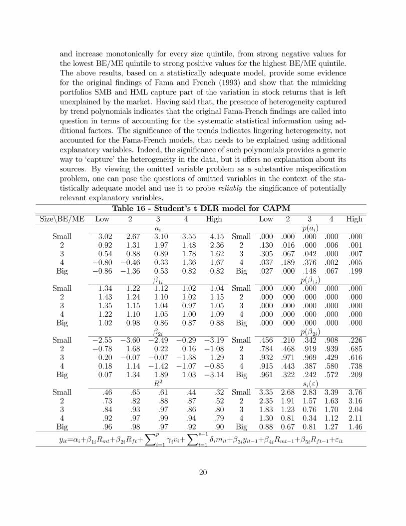
and increase monotonically for every size quintile, from strong negative values for

the lowest BE/ME quintile to strong positive values for the highest BE/ME quintile.

The above results, based on a statistically adequate model, provide some evidence

for the original findings of Fama and French (1993) and show that the mimicking

portfolios SMB and HML capture part of the variation in stock returns that is left

unexplained by the market. Having said that, the presence of heterogeneity captured

by trend polynomials indicates that the original Fama-French findings are called into

question in terms of accounting for the systematic statistical information using ad-

ditional factors. The significance of the trends indicates lingering heterogeneity, not

accounted for the Fama-French models, that needs to be explained using additional

explanatory variables. Indeed, the significance of such polynomials provides a generic

way to ‘capture’ the heterogeneity in the data, but it offers no explanation about its

sources. By viewing the omitted variable problem as a substantive mispecification

problem, one can pose the questions of omitted variables in the context of the sta-

tistically adequate model and use it to probe reliably the singificance of potentially

relevant explanatory variables.

Table 16 - Student’s t DLR model for CAPM

Size\BE/ME Low 2 3 4 High Low 2 3 4 High ()

Small 302 267 310 355 415 Small 000 000 000 000 0002 092 131 197 148 236 2 130 016 000 006 0013 054 088 089 178 162 3 305 067 042 000 0074 −080 −046 033 136 167 4 037 189 376 002 005Big −086 −136 053 082 082 Big 027 000 148 067 199

1 (1)Small 134 122 112 102 104 Small 000 000 000 000 0002 143 124 110 102 115 2 000 000 000 000 0003 135 115 104 097 105 3 000 000 000 000 0004 122 110 105 100 109 4 000 000 000 000 000Big 102 098 086 087 088 Big 000 000 000 000 000

2 (2)Small −255 −360 −249 −029 −319 Small 456 210 342 908 2262 −078 168 022 016 −108 2 784 468 919 939 6853 020 −007 −007 −138 129 3 932 971 969 429 6164 018 114 −142 −107 −085 4 915 443 387 580 738Big 007 134 189 103 −314 Big 961 322 242 572 209

2 ()Small 46 65 61 44 32 Small 335 268 283 339 3762 73 82 88 87 52 2 235 191 157 163 3163 84 93 97 86 80 3 183 123 076 170 2044 92 97 99 94 79 4 130 081 034 112 211Big 96 98 97 92 90 Big 088 067 081 127 146

=+1+2+X

=1+

X−1=1

+3−1+4−1+5−1+

20

Table 17 - Student’s t DLR model for three-factor model

Size\BE/ME Low 2 3 4 High Low 2 3 4 High ()

Small 137 063 094 113 157 Small 001 059 002 000 0002 −052 −060 002 −048 −028 2 140 029 946 073 3353 −045 −027 −056 032 −064 3 134 406 066 242 0864 −082 −099 −065 −020 −124 4 011 002 055 563 010Big 045 −059 058 −009 −022 Big 111 080 089 798 634

1 (1)Small 105 099 094 088 094 Small 000 000 000 000 0002 114 103 097 096 110 2 000 000 000 000 0003 113 103 099 098 105 3 000 000 000 000 0004 108 105 105 106 117 4 000 000 000 000 000Big 098 103 094 102 105 Big 000 000 000 000 000

2 (2)Small −131 −053 −055 064 −167 Small 412 664 614 529 0962 110 241 127 025 011 2 408 029 205 809 9233 169 −011 142 −089 178 3 150 925 248 394 2104 038 078 −060 026 −003 4 740 532 655 842 983Big 021 075 145 103 −158 Big 847 534 292 403 361

3 (3)Small 134 120 110 105 110 Small 000 000 000 000 0002 102 093 084 074 086 2 000 000 000 000 0003 076 064 056 045 067 3 000 000 000 000 0004 038 030 026 028 039 4 000 000 000 000 000Big −026 −020 −020 −016 −005 Big 000 000 000 000 183

4 (4)Small −023 006 021 033 055 Small 000 024 000 000 0002 −041 003 024 048 070 2 000 189 000 000 0003 −042 002 031 050 070 3 000 511 000 000 0004 −037 003 029 056 076 4 000 296 000 000 000Big −046 −003 021 057 082 Big 000 354 000 000 000

2 ()Small 07 35 46 46 27 Small 438 366 334 334 3872 40 64 71 73 53 2 353 271 245 236 3123 61 83 84 84 68 3 283 190 180 184 2564 85 91 93 88 75 4 176 135 119 158 227Big 91 98 94 87 80 Big 137 060 110 164 205

= + 1 + 2 + 3 + 4 +X

=1 +

X−1=1

+5−1 + 6−1 + 7−1 + 8−1 + 9−1 +

21

6 Summary and conclusionsUsing the distinction between a structural and a statistical model (often implicit)

the paper brings out the difference between substantive and statistical assumptions,

where the latter refer to the probabilistic assumptions imposed on the data, implicitly

or explicitly. This distinction enables one to separate the statistical from substantive

assumptions, such as ‘no relevant variables have been omitted’ from the estimated

model. It is argued that before one could reliably assess the empirical adequacy of

a structural model one needs to secure the validity of the statistical model. This is

because any form of statistical misspecification is likely to induce large discrepancies

between actual and nominal error probabilities. Hence, one should not rely on the

significance/nonsingnificance of coefficients to draw substantive inferences about the

adequacy of different theories.

This perspective is used to revisit the CAPM and the Fama-French three-factor

models with a view to assess their empirical adequacy. It was shown that the implicit

statistical models underlying these structural models are statistically misspecified.

That calls into question the empirical adequacy of the various extensions to the

CAPM because the significance of the additional terms was based on a statistically

misspecified models.

In addition, testing the over-identifying restrictions imposed by original CAPM

as well as the Fama-French extension, reveals that there is strong empirical evidence

against these structural models. This calls for a reconsideration of asset pricing

theories, more generally, with a view to explain the chance regularities found in stocks

returns. In particular, the strong lepotokurticity and the lingering heterogeneity need

to be accounted for by extending the Fama-French three-factor model with a view to

explain both features of the data.

Viewing the above empirical results from a theoretical perspective, it is clear that

some of the key assumptions of the CAPM as well as the Fama-French three-factor

model are rejected by the data. The Normality assumption, which provides the cor-

nerstone of these models as well as the Markowitz portfolio theory, is clearly rejected

by the data in favor of the Student’s t distribution. This constitutes a major break

from these theories primarily because of the heteroskedastic conditional variance of

the latter distribution. The presence of heterogeneity as well as temporal dependence

also call into question the assumption of equilibrium among agents using rational

expectations. The rejection of the adding-up restriction also calls into question the

basic tenet that the return to the risk free asset provides the comparison rod for

relating risks and returns.

22

References

[1] Banz, R. W. (1981), "The Relationship Between Return and Market Value of

Common Stocks". Journal of Financial Economics, 9(1): 3-18.

[2] Banz, R. W., & Breen, W. J. (1986), "Sample-Dependent Results Using Account-

ing and Market Data: Some Evidence". Journal of Finance, 41(4): 779-793.

[3] Basu, S. (1983), "The Relationship Between Earnings Yield, Market Value, and

Return for NYSE Common Stocks: Further Evidence". Journal of Financial

Economics, 12(1): 129-156.

[4] Bhandari, L. C. (1988), "Debt/Equity Ratio and Expected Common Stock Re-

turns: Empirical Evidence". Journal of Finance, 43(2): 507-528.

[5] Black, F. (1972), "Capital Market Equilibrium with Restricted Borrowing".

Journal of Business,45(3): 444-454.

[6] Black, F. (1993a), "Beta and Return". The Journal of Portfolio Management,

20(1), 8-18.

[7] Black, F. (1993b), "Estimating Expected Return". Financial Analysts Journal,

49(5): 36-38.

[8] Blume, M. E. (1970), "Portfolio Theory: A Step Toward its Practical Applica-

tion. Journal of Business,43(2): 152-173.

[9] Breeden, D. T. (1979), "An Intertemporal Asset Pricing Model with Stochastic

Consumption and Investment Opportunities". Journal of Financial Economics,

7(3): 265-296.

[10] Carhart, M. M. (1997), "On Persistence in Mutual Fund Performance". Journal

of Finance, 52(1): 57-82.

[11] Chen, N. F., Roll, R., and Ross, S. A. (1986), "Economic Forces and the Stock

Market". Journal of Business, 59(3): 383-403.

[12] Fama, E. F., and French, K. R. (1992), "The Cross-Section of Expected Stock

Returns". Journal of Finance, 47 (2): 427-465.

[13] Fama, E. F., and French, K. R. (1993), "Common Risk Factors in the Returns

on Stocks and Bonds". Journal of Financial Economics, 33(1): 3-56.

[14] Fang, K.-T., S. Kotz and K-W. Ng. (1990), Symmetric Multivariate and Related

Distributions, Chapman and Hall, London.

[15] Keim, D. B. (1983), Size-Related Anomalies and Stock Return Seasonality: Fur-

ther Empirical Evidence. Journal of Financial Economics, 12(1): 13-32.

[16] Kothari, S. P., Shanken, J. and Sloan, R. G. (1995), "Another Look at the

Cross-Section of Expected Stock Returns". Journal of Finance, 50(1): 185-224.

[17] Lehmann, E. L. (1986), Testing Statistical Hypotheses, 2nd ed., Wiley, NY

[18] Lintner, J. (1965a), "The Valuation of Risk Assets and the Selection of Risky

Investments in Stock Portfolios and Capital Budgets". Review of Economics and

Statistics, 73 : 13-37.

23

[19] Lintner, J. (1965b), "Security Prices, Risk and Maximal Gains from Diversifica-

tion". Journal of Finance, 20 : 587-615.

[20] Markowitz, H. (1952), "Portfolio Selection". Journal of Finance, 7(1): 77-91.

[21] Merton, R. C. (1973), "An Intertemporal Capital Asset Pricing Model". Econo-

metrica, 41(5): 867-887.

[22] Modigliani, F., and Miller, H. M. (1958), "The Cost of Capital, Corporation

Finance and the Theory of Investment". American Economic Review, 48(3):

261-297.

[23] Mossin, J. (1966), "Equilibrium in a Capital Asset Market". Econometrica, 34

(4): 768-783.

[24] Rosenberg, B., Reid, K., and Lanstein, R. (1985), "Persuasive Evidence of Mar-

ket Inefficiency". Journal of Portfolio Management, 11(3): 9-17.

[25] Roll, R. (1983), "The turn of the year effect and the return premia of small

firms". Journal of Portfolio Management, 9, 18-28.

[26] Ross, S. A. (1976), "The Arbitrage Theory of Capital Asset Pricing". Journal of

Economic Theory, 13(3): 341-360.

[27] Sharpe, W. F. (1964), "Capital Asset Prices: A Theory of Market Equilibrium

under Conditions of Risk". Journal of Finance, 19(3): 425-442.

[28] Spanos, A., (1986), Statistical Foundations of Econometric Modelling, Cam-

bridge University Press, Cambridge.

[29] Spanos, A. (1990), “The Simultaneous Equations Model revisited: statistical

adequacy and identification”, Journal of Econometrics, 44, 87-108.

[30] Spanos, A. (1994), “On Modeling Heteroskedasticity: the Student’s t and Ellip-

tical Linear Regression Models,” Econometric Theory, 10: 286-315.

[31] Spanos, A. (1999), Probability Theory and Statistical Inference: econometric

modeling with observational data, Cambridge University Press, Cambridge.

[32] Spanos, A. (2006a), “Where Do Statistical Models Come From? Revisiting

the Problem of Specification,” pp. 98-119 in Optimality: The Second Erich L.

Lehmann Symposium, edited by J. Rojo, Lecture Notes-Monograph Series, vol.

49, Institute of Mathematical Statistics.

[33] Spanos, A. (2006b), “Revisiting the omitted variables argument: substantive vs.

statistical adequacy,” Journal of Economic Methodology, 13: 179—218.

[34] Spanos, A. (2009), “Statistical Misspecification and the Reliability of Inference:

the simple t-test in the presence of Markov dependence,” Korean Economic Re-

view, 25: 165-213.

[35] Spanos, A. (2010), “Statistical adequacy and the trustworthiness of empirical ev-

idence: Statistical vs. substantive information”, Economic Modelling, 27: 1436—

1452.

24

[36] Spanos, A. and A. McGuirk (2001), “The Model Specification Problem from

a Probabilistic Reduction Perspective,” Journal of the American Agricultural

Association, 83: 1168-1176.

[37] Tobin, J. (1958), "Liquidity Preference as Behavior Towards Risk". Review of

Economic Studies, 25(2), 65-86.

[38] Treynor, J. L. (1999), "Toward a Theory of Market Value of Risky assets". Robert

Korajczyk (Ed.), Asset Pricing and Portfolio Performance. London: Risk Books.

25

7 Appendix - M-S results7.1 Appendix A: M-S results for assumption [1]

Table A1 - M-S results for Normal/Linear Regression (LR) model

The M-S testing of Normal LR model assumption [1] in table 1 is tested by

adapting the Shapiro-Wilk (S-W), Anderson-Darling (A-D) and D’Agostino-Pearson

(D’AP); July 1963 to December 1991, 342 months.

Size\BE/ME Low 2 3 4 High Low 2 3 4 High

=+1+2+ =1 2 ∈N[11] Shapiro-Wilk ( ) ( )

Small 0991 0986 0974 0968 0950 Small 026 002 000 000 0002 0988 0974 0979 0969 0964 2 006 000 000 000 0003 0986 0992 0973 0978 0967 3 002 074 000 000 0004 0988 0985 0962 0976 0986 4 005 002 000 000 002Big 0992 0997 0971 0992 0970 Big 073 747 000 060 000

[12] Anderson-Darling (2) (2)Small 1088 1274 2279 3176 3405 Small 007 003 000 000 0002 0573 1791 2001 1619 1975 2 136 000 000 000 0003 0345 0457 1886 1435 1773 3 483 264 000 001 0004 0656 1477 2345 1753 0682 4 086 001 000 000 074Big 0795 0222 1934 0597 1301 Big 039 830 000 118 002

[13] D’Agostino-Pearson (2) (2)Small 8999 13916 25816 29520 67249 Small 011 001 000 000 0002 13773 33953 17600 39012 41735 2 001 000 000 000 0003 17229 9205 23956 20479 42499 3 000 010 000 000 0004 10860 9685 34695 29688 16051 4 004 008 000 000 000Big 7172 1022 37272 9064 25767 Big 028 600 000 011 000

=+1+2+3+4+ =1 2 ∈N[11] Shapiro-Wilk ( ) ( )



[13] D’Agostino-Pearson (2) (2)Small 13536 1488 4388 5835 9934 Small 001 475 111 054 0072 14101 21517 3238 1982 6207 2 001 000 198 371 0453 5782 3160 10842 2143 10435 3 056 206 004 343 0054 4131 7974 14789 14233 0836 4 127 019 001 001 658Big 4841 0005 51126 4045 14580 Big 089 998 000 132 001

26

Table A2 - M-S results for Student’s t VAR(1; =4) model

The M-S testing of Student’s t VAR(1; =4) model assumption [1] in table 12

is tested by adapting the Kolmogorov-Smirnov (K-S) and Anderson-Darling (A-D);

July 1963 to December 1991, 342 months.

Size\BE/ME Low 2 3 4 High Low 2 3 4 High

=+X

=1+

X−1=1

+1−1+2−1+3−1+ =1 2 ∈N[11] Kolmogorov-Smirnov () ()



=+X

=1+

X−1=1




=+X

=1+

X−1=1




27

7.2 Appendix B: M-S results for assumptions [2]-[5]

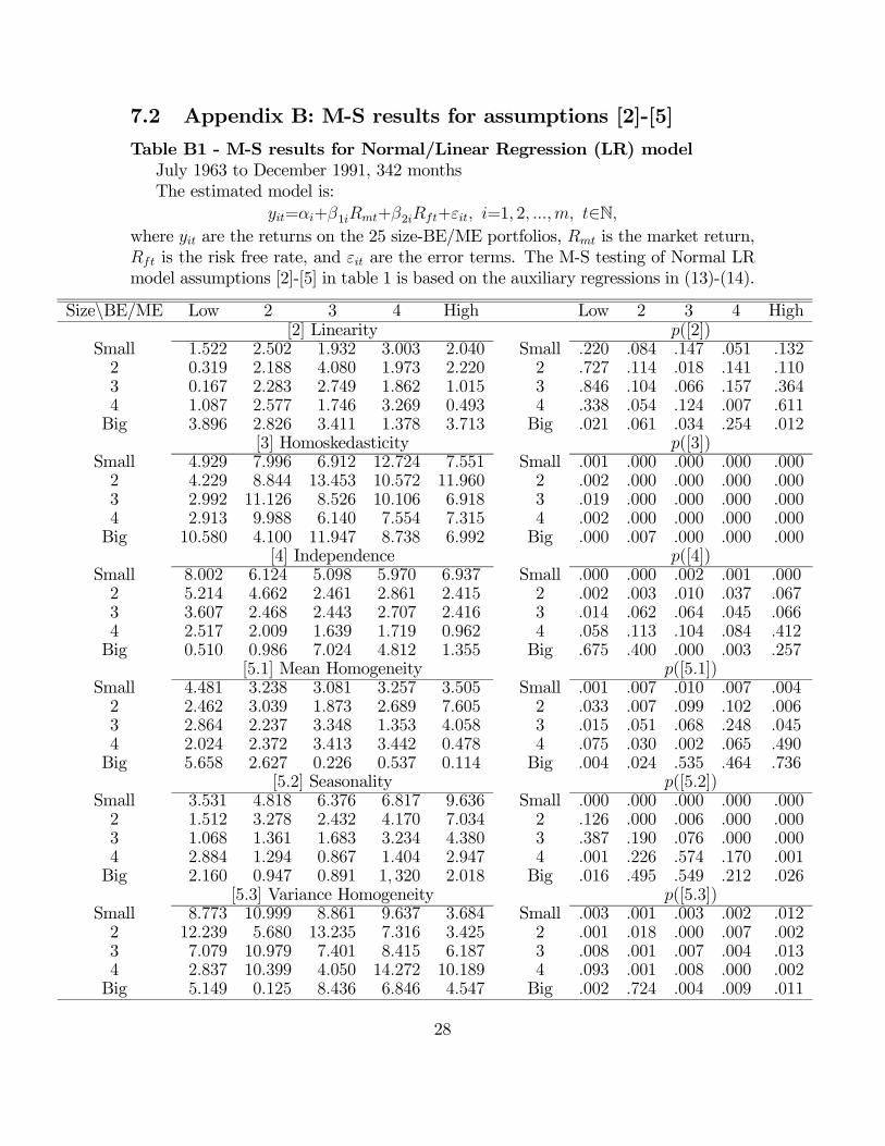
Table B1 - M-S results for Normal/Linear Regression (LR) model

July 1963 to December 1991, 342 months

The estimated model is:

=+1+2+ =1 2 ∈Nwhere are the returns on the 25 size-BE/ME portfolios, is the market return,

is the risk free rate, and are the error terms. The M-S testing of Normal LR

model assumptions [2]-[5] in table 1 is based on the auxiliary regressions in (13)-(14).

Size\BE/ME Low 2 3 4 High Low 2 3 4 High[2] Linearity ([2])


[3] Homoskedasticity ([3])Small 4929 7996 6912 12724 7551 Small 001 000 000 000 0002 4229 8844 13453 10572 11960 2 002 000 000 000 0003 2992 11126 8526 10106 6918 3 019 000 000 000 0004 2913 9988 6140 7554 7315 4 002 000 000 000 000Big 10580 4100 11947 8738 6992 Big 000 007 000 000 000

[4] Independence ([4])Small 8002 6124 5098 5970 6937 Small 000 000 002 001 0002 5214 4662 2461 2861 2415 2 002 003 010 037 0673 3607 2468 2443 2707 2416 3 014 062 064 045 0664 2517 2009 1639 1719 0962 4 058 113 104 084 412Big 0510 0986 7024 4812 1355 Big 675 400 000 003 257

[51] Mean Homogeneity ([51])Small 4481 3238 3081 3257 3505 Small 001 007 010 007 0042 2462 3039 1873 2689 7605 2 033 007 099 102 0063 2864 2237 3348 1353 4058 3 015 051 068 248 0454 2024 2372 3413 3442 0478 4 075 030 002 065 490Big 5658 2627 0226 0537 0114 Big 004 024 535 464 736

[52] Seasonality ([52])Small 3531 4818 6376 6817 9636 Small 000 000 000 000 0002 1512 3278 2432 4170 7034 2 126 000 006 000 0003 1068 1361 1683 3234 4380 3 387 190 076 000 0004 2884 1294 0867 1404 2947 4 001 226 574 170 001Big 2160 0947 0891 1 320 2018 Big 016 495 549 212 026

[53] Variance Homogeneity ([53])Small 8773 10999 8861 9637 3684 Small 003 001 003 002 0122 12239 5680 13235 7316 3425 2 001 018 000 007 0023 7079 10979 7401 8415 6187 3 008 001 007 004 0134 2837 10399 4050 14272 10189 4 093 001 008 000 002Big 5149 0125 8436 6846 4547 Big 002 724 004 009 011

28

Table B2 - M-S results for Normal/Linear Regression (LR) model



=+1+2+3+4+ =1 2 ∈Nwhere are the returns on the 25 size-BE/ME portfolios, is the market return,

is the risk free rate, and are the Fama-French size and value factors,

and are the error terms. The M-S testing of Normal LR model assumptions [2]-[5]

in table 1 is based on the auxiliary regressions in (13)-(14).



[3] Homoskedasticity ([3])Small 3482 2812 1474 1887 5790 Small 001 005 113 027 0002 3374 4772 2211 4003 1996 2 000 000 003 003 0183 2747 5555 2748 3798 1814 3 000 000 006 000 1264 2420 4421 2936 3108 0895 4 009 000 000 002 530Big 5840 9073 4074 4249 8273 Big 000 000 000 000 000

[4] Independence ([4])Small 4130 3784 1590 1551 3991 Small 001 002 163 174 0022 2992 0985 1649 0865 0921 2 012 427 060 505 4683 3024 1950 1232 2883 0359 3 001 038 270 015 8764 2239 0371 1337 2137 2290 4 016 868 210 008 046Big 1597 0479 3093 3343 2017 Big 161 792 010 006 076

[51] Mean Homogeneity ([51])Small 2426 0828 6329 1962 0036 Small 048 364 012 162 8502 0543 2029 2994 0545 2207 2 462 074 085 461 1383 1683 0010 0417 0075 0672 3 196 921 519 784 4134 0085 0025 1864 0370 2534 4 771 876 075 544 029Big 1873 1347 1967 0323 0400 Big 172 247 070 570 527

[52] Seasonality ([52])Small 2973 1657 2408 2978 4302 Small 001 082 007 001 0002 2229 1031 1119 1499 1143 2 013 419 345 131 3273 1517 0930 2160 1708 1423 3 124 511 016 071 1614 2345 2153 1040 13191 0884 4 009 017 411 000 557Big 1924 0553 1476 0743 1180 Big 036 866 139 697 300

[53] Variance Homogeneity ([53])Small 1514 3004 0661 0130 1861 Small 185 051 417 719 1742 7843 2234 10213 2508 3270 2 005 051 002 114 0393 2389 7136 7652 5286 3312 3 038 008 006 022 0204 1857 12335 4375 3788 1946 4 102 001 005 052 086Big 3088 2346 1610 2952 4381 Big 016 024 205 008 005

29

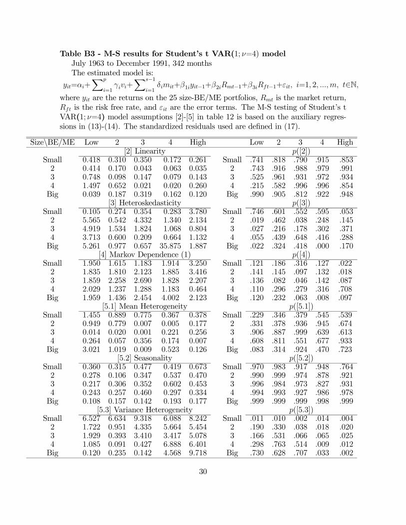
Table B3 - M-S results for Student’s t VAR(1; =4) model



=+X

=1+

X−1=1

+1−1+2−1+3−1+ =1 2 ∈Nwhere are the returns on the 25 size-BE/ME portfolios, is the market return,

is the risk free rate, and are the error terms. The M-S testing of Student’s t

VAR(1; =4) model assumptions [2]-[5] in table 12 is based on the auxiliary regres-

sions in (13)-(14). The standardized residuals used are defined in (17).



[3] Heteroskedasticity ([3])Small 0105 0274 0354 0283 3780 Small 746 601 552 595 0532 5565 0542 4332 1340 2134 2 019 462 038 248 1453 4919 1534 1824 1068 0804 3 027 216 178 302 3714 3713 0600 0209 0664 1132 4 055 439 648 416 288Big 5261 0977 0657 35875 1887 Big 022 324 418 000 170

[4] Markov Dependence (1) ([4])Small 1950 1615 1183 1914 3250 Small 121 186 316 127 0222 1835 1810 2123 1885 3416 2 141 145 097 132 0183 1859 2258 2690 1828 2207 3 136 082 046 142 0874 2029 1237 1288 1183 0464 4 110 296 279 316 708Big 1959 1436 2454 4002 2123 Big 120 232 063 008 097

[51] Mean Heterogeneity ([51])Small 1455 0889 0775 0367 0378 Small 229 346 379 545 5392 0949 0779 0007 0005 0177 2 331 378 936 945 6743 0014 0020 0001 0221 0256 3 906 887 999 639 6134 0264 0057 0356 0174 0007 4 608 811 551 677 933Big 3021 1019 0009 0523 0126 Big 083 314 924 470 723


[53] Variance Heterogeneity ([53])Small 6527 6634 9318 6088 8242 Small 011 010 002 014 0042 1722 0951 4335 5664 5454 2 190 330 038 018 0203 1929 0393 3410 3417 5078 3 166 531 066 065 0254 1085 0091 0427 6888 6401 4 298 763 514 009 012Big 0120 0235 0142 4568 9718 Big 730 628 707 033 002

30




=+X

=1+

X−1=1












31




=+X

=1+

X−1=1












32

validating the capm and the fama-french three-factor · pdf filethe latter limitation,...

Documents