validating the accuracy of heat source model via temperature

International Journal of Engineering & Technology IJET-IJENS Vol: 11 No: 05 12

111505-6868 IJET-IJENS @ October 2011 IJENS I J E N S

Abstract—Welding process generally is modeled as a moving

heat source over a solid. This paper used Goldak’s ellipsoidal moving heat source model. Goldak has proposed a volumetric heat source model according to the mathematical expressions:

2

2

2

2

2

2 333

'''),,(

36zyx rr

y

r

x

zyx

yx eeerrr

qq

ξ

ξ ππ

−−−

⋅⋅=&

& . For a known heat

input value, crucial parameters of the Goldak’s heat source model are rx, ry and rz. Using rx, ry and rz equal to 5mm, 2mm and 3mm respectively; a well match temperature histories with experimental result at observed positions and weld pool shape can be obtained.

Index Terms—Goldak’s heat source models, temperature history, temperature field

I. INTRODUCTION

ANY benefits can be achieved through welding simulation. Production cost can be reduced by limiting

try and error of experimental welding. Using simulation, welding risk can be minimized in the earliest stage of the product development cycle. Welding simulation can also ascertain the level and distribution of residual stresses [1]. Welding simulation can be used as a tool for study such as material behaviors under welding phenomenon [2], the effects of weld metal yield strength to residual stress [3] and the roles of phase transformation in the residual stress development [4]. Welding simulation is proposed to be used as assessment tool [5], and it is expected welding simulation to be used as a complement of experiment procedure in determining Welding Procedure Standard (WPS) [6].

Welding process is modeled as a moving heat source over a solid. Heat source can be modeled as a point heat source [7,8]. Point heat source is heat load with value equal to generated heat q& (J/s) over a nodal at a solid. Heat source may be

modeled as a surface heat source "q& (J/m2s) [4,9,10]. Surface

heat source is heat flux that is heat generated over certain area. The heat flux can be uniformly distributed or distributed according to Gaussian distribution. Heat source can also be

Manuscript received October 9, 2001. Djarot B. Darmadi is a Brawijaya University - Indonesia lecturer, he is

studying at University of Wollongong – Australia (e-mail : [email protected] or [email protected] )

represented as a volumetric heat source '''q& (J/m3s) [11,12].

Volumetric heat source is a body heat load applies for certain volume. As in surface heat source, volumetric heat source can be uniformly distributed or distributed according to certain pattern.

The welding process involves many different phenomenon namely thermal, mechanical and metallurgical phenomenons. In thermal model heat input from heat source is used to heat and melt the welded metal. The heat is conducted away from the heat source into base metal and the heat is lost to the environment by convection and radiation and also by conduction to contacting bodies. In thermal model temperature history of certain node and temperature field for certain time can be observed.

Analysis of welding process is often considered as a coupled problem. When thermal model is coupled by mechanical model, the analysis is usually called as Thermo-Mechanical analysis (TM). Most analysis is performed in two steps: thermal analysis followed by mechanical analysis. In TM analysis temperature distribution in thermal analysis is used as thermal load. Strain and stress as a function of time because of the thermal load can be observed. Usually the effect of mechanical model to thermal model is neglected. For certain material, solid state phase transformation exists when heated to such high temperature as in welding process. Since phase transformation affects thermal and mechanical properties of the welded material, it should be included in the analysis. If the analysis includes phase transformation considerations, the analysis is called as Thermo-Mechanical-Metallurgical (TMM) analysis.

No matter until what extend the analysis will be carried out, thermal analysis as a basic of welding phenomenon should be correct. The most important thing in the thermal analysis is the heat source model. The defects on the heat source model mislead the next analysis. In this paper the accurate model of heat source of bead-on-plate welding is proposed. The validation is done by observing temperature histories of measured nodes and comparing the predicted and measured weld-pool shape.

II. GAUSSIAN SURFACE HEAT SOURCE MODEL

Since heat torch transmits heat over a surface, surface heat source (heat flux) is closer to the real condition than point heat

Validating the accuracy of heat source model via temperature histories and temperature field in

bead-on-plate welding

Djarot B. Darmadi

M



source. Instead of uniformly distributed, many researchers have used distributed surface disc heat source model according to Gauss distribution. For Gaussian distributed heat source, heat at certain distance (r i) from heat source centre has value according to equation 1.

( )2/"

0" oi rrCi eqq −= && (1)

where "

0q& is heat flux generated at the center of heat source

model, ro is the outer disc radius and C is an arbitrarily constants. It is generally assumed that the heat value at the outer radius is 5% of the maximum heat at the center of heat source. Using this assumption, the constant C is closed to 3 and equation (1) can be represented as in equation 2.

( )2/3"

0" oi rri eqq −= && (2)

In Cartesian x-y coordinate system, equation (2) can be

expressed as in equation (3).

2

2

2

2 33

"0

" oo r

y

r

x

i eeqq−−

⋅= && (3)

III. GOLDAK VOLUMETRIC HEAT SOURCE MODEL

The volumetric moving heat source model is pioneered by Goldak et.al. [13]. The existence of digging and stirring of arc welding such as distributed pressure, surface tension and buoyancy forces have been known in practical welding. Since all of those phenomenons are distributed throughout a volume of material, Goldak introduced volumetric heat source. The relation between welding physics and volumetric heat source model is well described by Gilles et.al. [14] as shown at figure 1.

If the welding process moves parallel to the z axis, and ξ

represents a moving abscissa parallel to the z axis, the heat load at a certain small increment volume inside an ellipsoid can be expressed by distributed volumetric heat load as expressed by equation (4).

222'''0),,('''

ξξ

CByAxyx eqq −−−= && (4)

A, B and C are constants; '''

0q& is volumetric heat source

generated at heat source center. For simplification, Goldak assumed weld plate as an infinite solid. Considering energy conservation and that welding applied on a plate, i.e. semi infinite solid, equation (5) is obtained.

∫ ∫ ∫∞ ∞ ∞

−−−==0 0 0

'''0

222

822 ξη ξ dxdydeqVIq CByAx& (5)

where η is welding efficiency, V is voltage (volt) and I is electrical current (amp).

It is known mathematically that )(.212

terfdtet π=∫ , and

at the limits π21

0

2

=∫∞

− dte t . As a result equation (5) can be

written as in (6).

ABC

qq

ππ'''02 =& (6)

Analog to Gaussian distributed surface heat source model,

the ratio between the minimum heat flux at the center of ellipsoid and maximum heat flux at the ellipsoid center is taken as 5%. Hence for elements at (rx,0,0), (0,ry,0) and (0,0,rz) '''

0"

),,( %5 qq yx && =ξ ; and using equation (4) and (6),

equation (7) can be obtained for the Goldak heat source model.

2

2

2

2

2

2 333

'''),,(

36zyx rr

y

r

x

zyx

yx eeerrr

qq

ξ

ξ ππ

−−−

⋅⋅=&

& (7)

The maximum value of equation (7) is zyx rrr

qq

ππ&

&36'''

0 = at

position (0,0,0). Considering this condition and substituting

2

2

2

2

2

22 333

zyxe rr

y

r

xr

ξ++= , equation (7) can be simplified to

equation (8).

2'''0

'''),,(

eryx eqq −= && ξ (8)

IV. EXPERIMENT PROCEDURE BY NET

A major issue in modeling is accuracy and validity. To this end the European Network on Neutron Techniques Standardization for Structural Integrity (NeT) has published experimental data and procedures which can be accessed at https://odin.jrc.ec.europa.eu [15,16]. Experimental work was carried out using bead-on-plate (bop) welding. Nine thermocouples were attached at different measured points. The



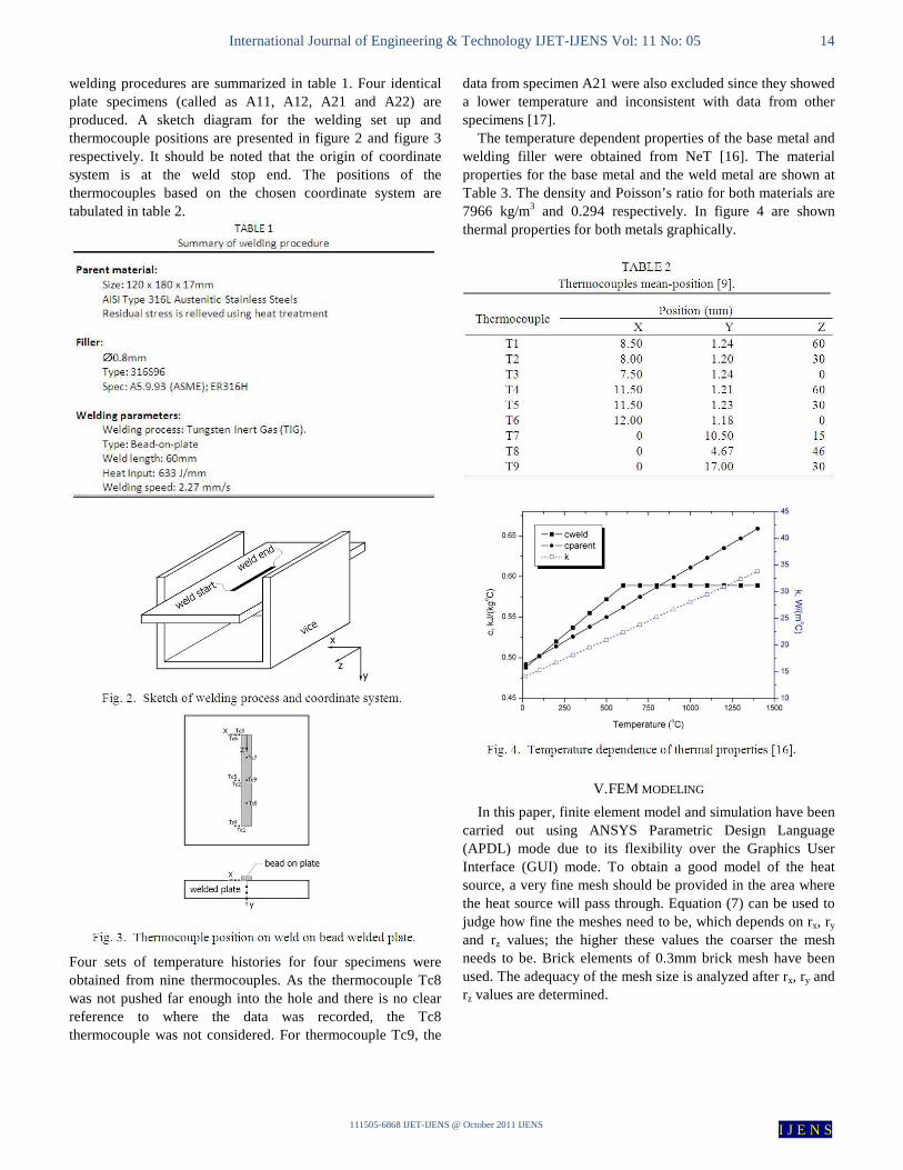
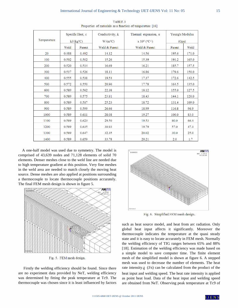
welding procedures are summarized in table 1. Four identical plate specimens (called as A11, A12, A21 and A22) are produced. A sketch diagram for the welding set up and thermocouple positions are presented in figure 2 and figure 3 respectively. It should be noted that the origin of coordinate system is at the weld stop end. The positions of the thermocouples based on the chosen coordinate system are tabulated in table 2.

Four sets of temperature histories for four specimens were obtained from nine thermocouples. As the thermocouple Tc8 was not pushed far enough into the hole and there is no clear reference to where the data was recorded, the Tc8 thermocouple was not considered. For thermocouple Tc9, the

data from specimen A21 were also excluded since they showed a lower temperature and inconsistent with data from other specimens [17].

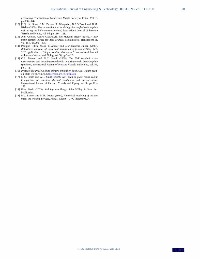
The temperature dependent properties of the base metal and welding filler were obtained from NeT [16]. The material properties for the base metal and the weld metal are shown at Table 3. The density and Poisson’s ratio for both materials are 7966 kg/m3 and 0.294 respectively. In figure 4 are shown thermal properties for both metals graphically.

V. FEM MODELING

In this paper, finite element model and simulation have been carried out using ANSYS Parametric Design Language (APDL) mode due to its flexibility over the Graphics User Interface (GUI) mode. To obtain a good model of the heat source, a very fine mesh should be provided in the area where the heat source will pass through. Equation (7) can be used to judge how fine the meshes need to be, which depends on rx, ry and rz values; the higher these values the coarser the mesh needs to be. Brick elements of 0.3mm brick mesh have been used. The adequacy of the mesh size is analyzed after rx, ry and rz values are determined.



A one-half model was used due to symmetry. The model is comprised of 43,639 nodes and 71,128 elements of solid 70 elements. Denser meshes close to the weld line are needed due to high temperature gradient at this position. Very fine meshes in the weld area are needed to match closely the moving heat source. Dense meshes are also applied at positions surrounding a thermocouple to locate thermocouple positions accurately. The final FEM mesh design is shown in figure 5.

Firstly the welding efficiency should be found. Since there

are no experiment data provided by NeT, welding efficiency was determined by fitting the peak temperature at Tc9. The thermocouple was chosen since it is least influenced by factors

such as heat source model, and heat from arc radiation. Only global heat input affects it significantly. Moreover the thermocouple indicates the temperature at the quasi steady state and it is easy to locate accurately in FEM mesh. Normally the welding efficiency of TIG ranges between 65% and 88% [18]. Estimation of the welding efficiency was made based on a simple model to save computer time. The finite element mesh of the simplified model is shown at figure 6. A stepped mesh was used to decrease the number of elements. The heat rate intensityq& (J/s) can be calculated from the product of the

heat input and welding speed. The heat rate intensity is applied as point heat load. Data of the heat input and welding speed are obtained from NeT. Observing peak temperature at Tc9 of



the simulation result on simplified model, the welding efficiency was found to be 76%. Convection coefficient and emissivity are assumed to be 5 W/m2.K° and 0.5 respectively. Ambient temperature is assumed as 25°C based on the averages of thermocouple measurements. Heat source parameters (rx, ry, rz) are varied as (3mm, 3mm, 3mm), (5mm, 3mm, 3mm), (5mm, 2mm, 3mm) and (5mm, 2mm, 2mm). Temperature histories and temperature field are evaluated again experiment data provided by NeT.

Brick mesh sizes along the heat source trajectory are 0.3mm. The body heat source values depend on the distance from the centroid of the elements to the center of the heat source. Since the brick mesh sizes are 0.3mm and applying to equation (7), comparison between '''

0'''

),,( / qq yx && ξ for each heat

source model is presented at table 4. The least value is 97.90 for [5,2,2] model which means the maximum body heat will be represented by 97.90% of its value, and it can be assumed that the mesh size along the weld path is sufficiently fine.

The welding simulation used element birth-and-death

technique approach. In the element birth and death technique, the metal bead is growing with the moving heat source. First, all of weld bead elements are “omitted” using EKILL command in ANSYS-APDL and the growth is modeled using EALIVE command. Born elements are elements of the weld bead which are already left behind the moving heat source. When the elements are born, their temperature should be at the melting embedded filler metal temperature which is superheated at 2400°C [19]. Instead of applying temperature node load, the body heat load rate ('''q& ) at elements was

applied. The body heat load value is such that it can produce a temperature of 2400°C at the growing weld bead. The heat needed to elevated the weld pool from the initial temperature of 25°C to 2400°C was evaluated using q = mc∆T. It should be noted that the specific heat c, is temperature-dependent as expressed in Table 3b. The specific heat at a certain temperature range was taken as the mean value between these

ranges. The heat rate can be obtained using

∆=v

STmcq&

expression. Finally, the body heat load which should be applied at the born weld bead can be obtained using equation (9).

∆=v

STcq ρ'''& (9)

VI. RESULTS AND DISCUSSIONS

Temperature histories for varied heat source model are compared as shown in figure 7. Figure 7a, 7b and 7c describe temperature histories for thermocouple at the top surface. In figure 7a are compared temperature histories at weld start point, Tc1 for the closer thermocouple and Tc4 for the farther one. Tc1 peak temperature are 245.127°C, 257.742°C, 254.748°C and 251.251.183°C for [3, 3, 3], [5, 3, 3], [5, 2, 3] and [5, 2, 2] respectively. All of those peak temperatures are achieved when t = 6.495s except for [3, 3, 3] heat source model which, is obtained when t = 7.024s. Tc4 peak temperature are 142.980°C, 146.441°C, 145.543°C and 144.111°C when time equal to 11.783s, 11.254s, 11.254s and 11.254s for those [3, 3, 3], [5, 3, 3], [5, 2, 3] and [5, 2, 2] respectively.

Three important notes can be underlined here, first is that the model with rx = 3mm showed split results with others in term of peak temperature and when (time) the peak temperature is achieved. Variation in the other heat source model (ry and rz) does not show significant difference. Regarding the coordinate system shown at figures 2 and 3, rx is the size of ellipsoidal heat source model in the transversal direction parallel to the surface of the base metal. Tc1 and Tc4 are the positions at surface those perpendicular to the weld line. It may be the reason why rx affects the temperature histories of the thermocouple in the coincide direction. Evaluating standard deviation for Tc1 and Tc4, those are 5.420 and 1.531 respectively. This means Tc1 is more susceptible to heat source model than Tc4; it is the second notes that the closer position is more affected by the heat source model than the farther one. The last but not the least note is that using lower rx produces lagging time of the peak temperature. Since the thermocouple is farther from heat source model for the lower rx the longer time is needed for the heat from the heat source model to reach the observed position. Using rx = 3mm the peak temperature for Tc1 is achieved at 7.024s whilst for rx = 5mm is at 6.495s that lagging by 0.529s. Evaluating temperature histories for Tc4, peak temperature for rx = 3mm is at 11.783 whilst for rx = 5mm is at 11.254s. Again the peak temperature with rx = 3mm is lagging by 0.529s. The other insight which may also precious is when evaluation is done for the same heat source model but for different position (Tc1 and Tc4). Evaluating rx = 3mm peak temperatures are at 7.024s and at 11.783s for Tc1 and Tc4 respectively. Longer time for peak temperature of Tc4 is caused by the farther position than Tc1. The time for peak temperatures differ by 4.759s. Using rx = 5mm peak temperature for Tc1 and Tc4 are at 6.495s and 11.254 which also differ by 4.759s with time lagging for Tc4 due to it farther position to the heat source center.



Figure 7b describes temperature histories for position in the

middle of weld bead, Tc2 and Tc5 for closer and farther position respectively. In figure 7c are shown temperature histories for thermocouple at the weld end point, for the closer (Tc3) and farther (Tc6) one. The peak temperatures and the times when the peak temperatures is produced for varied heat source model and for different position are summarized at table 5. The same conclusions with thermocouple on the start point for middle and end point thermocouples can be derived. Peak temperatures at the middle position show higher values than the start point thermocouples for the same heat source model. That higher temperature as a result of the facts that the middle position has been preheated by the heat source center before the heat source center derived middle thermocouples z coordinates.

The lower peak temperatures (compare to the middle thermocouple) are exhibited by the thermocouple at the weld end. Although the end point thermocouple are also preheated, but the weld torch is extinguished instantaneously when the weld torch center arrives at the end point. This sudden extinction causes the lower peak temperature.

Next evaluation is done for thermocouple inside the base metal (Tc7) and bottom-surface thermocouple (Tc9). Peak temperature and time for the peak temperature for [3, 3, 3], [5, 3, 3], [5, 2, 3] and [5, 2, 2] heat source models at Tc7 are 256.639°C, 254.720°C, 252.970°C and 252.289°C respectively which all achieved at 30.043s. The standard deviation for the peak temperatures is 1.947. The low standard

deviation means no significant affect is observed because of the heat source model variation. For the Tc9 the peak temperatures are 200.593°C, 200.577°C, 199.298°C and 198.351°C at 33s. The standard deviation is even lower than the standard deviation for Tc7 (1.087).

Temperature field at the mid-plate cross section are shown at figure 8 for varied heat source model. The picture describes temperature fields when heat source exactly at the middle of the plate, thus it shows the maximum temperature at the cross section position. It should be noted that the melting temperature of the base metal is 1400°C which means isothermal line for 1400°C also shows weld pool shape. Observing figure 8, arrives to conclusion that heat source model with rx, ry and rz equal to 5mm, 2mm and 3mm respectively gives better weld pool shape than the others. With the heat source model, the 1400°C isothermal lines have the width equal to the weld-bead.

The next comparison is made between experimental result with thermal model of [5,2,3] heat source. In figure 9 is shown comparison between weld-pool shape from [5,2,3] heat source model and from experimental results. It can be said that the FEM model of weld pool shape shown good agreement with the experimental result. Not only has the width of the weld-pool matched the experimental cross section but also the depth of the weld pool.

In figure 10 temperature history from [5,2,3] heat source model is compared to the experimental results. Four sets of experimental temperature histories are obtained from four specimens (A11, A12, A21 and A22). From these figures it can be concluded that FEM simulation has shown a good agreement with experimental results. Apart from showing the general trend, the transient temperature values generally also match the experimental data. For the close field thermocouples, the FEM model predicts a lower temperature than the measured peak temperature. The lower prediction may be caused by the radiation of torch arc which was not modeled. The ‘below bead’ thermocouple (Tc7) from FEM model shows a higher value than that measured by the thermocouple. The



‘below bead’ thermocouple was inserted 6.5mm deep in a hole with diameter of 1.2mm. The possibility that the thermocouple is not fully located at the tip of the hole is high. Incomplete insertion could result in a larger distance from the heat source and a lower measured peak temperature. If the measured point is only 0.5mm farther from the heat source, simulation using the ANSYS model showed that the peak temperature will fit with the measured peak temperature.

VII. CONCLUSION

Varied heat source model has no significant difference for temperature histories at observed positions, however small different is shown at thermocouples close to the weld-bead. Temperature field for close positions and weld pool shape are significantly affected by heat source model. Observing temperature histories and weld pool shape, heat source model with rx, ry and rz equal to 5mm, 2mm and 3mm respectively gives well match results with experimental data.

VIII. FUTURE WORKS

Practically, mechanical properties of resulted welding joint are more preferable than thermal results (temperature history or temperature field). The typical recent topic of interest of the mechanical properties is residual stress. Discussion on residual stress using the above validated thermal model will be a precious work.

REFERENCES

[1] ESI Group Released Notes (2006), The welding simulation solution, p.4.

[2] Andrea Capriccioli, Paolo Frosi (2009), Multipurpose ANSYS FE procedure for welding processes simulation, Fusion Engineering and Design vol. 84 pp. 546 – 553.

[3] Dean Deng, Hidekazu Murakawa and Wei Liang (2008), Numerical and experimental investigations on welding residual stress in multi-pass butt-welded austenitic stainless steel pipe, Computational Material Science, vol.42, pp.234-244.

[4] Deng Dean, Murakawa Hidekazu (2006), Prediction of welding residual stress in multi-pass-butt-welded modified 9Cr-1Mo steel pipe considering phase transformation effects, Computational Materials Science, vol.37, pp. 209 – 219.

[5] Viorel Deaconu (2007), Finite element modeling of residual stress – a powerful tool in the aid of structural integrity assessment of welded structures, 5th Int. Conference Structural Integrity of Welded Structures, pp.1 - 9, Romania.

[6] Lars-Erik Lindgren (2001), Finite element modeling and simulation of welding part 1: increased complexity, Journal of Thermal Stresses, vol. 24, pp. 141 – 192.

[7] M. Van Elsen, M. Baelmans, P. Mercelis and J.P. Kurth (2007), Solution for modeling moving heat source in a semi-infinite medium and application to laser material processing, International Journal of Heat and Mass Transfer, vol. 50, pp.4872 – 4882.

[8] S. Dragi and V. Ivana (2009), Finite element analysis of residual stress in butt welding two similar plates, Scientific Technical Review, vol.59, no.1, pp. 57 – 60.

[9] Z. Chai, H. Zhao and A. Lu (2003), Efficient finite element approach for modeling of actual welded structures, Science and Technology of Welding and Joining, vol.8, no.3, pp. 195 – 204.

[10] F. Lu, S. You and Y. Li (2004), Modeling and finite element analysis on GTAW arc and weld pool, Computational Materials Science, Vol.29, pp.371 -278.

[11] Lei Yu-cheng, Yu Wen-xia, Li Chai-hui and Cheng Xiao-nong (2006), Simulation on temperature field of TIG welding of cooper without



preheating, Transaction of Nonferrous Metals Society of China, Vol.16, pp.838 – 842.

[12] [12] X. Shan, C.M. Davies, T. Wangsdan, N.P.O’Dowd and K.M. Nikbin (2009), Thermo-mechanical modeling of a single-bead-on-plate weld using the finite element method, International Journal of Pressure Vessels and Piping, vol. 86, pp.110 – 121.

[13] John Goldak, Aditya Chakravarti and Malcolm Bibby (1984), A new finite element model for heat sources, Metallurgical Transactions B, vol. 15B, pp.299 – 305.

[14] Philippe Gilles, Walid El-Ahmar and Jean-Francois Jullien (2009), Robustness analyses of numerical simulation of fusion welding NeT-TG1 application : “Single weld-bead-on-plate”, International Journal of Pressure Vessels and Piping, vol.86, pp.3 – 12.

[15] C.E. Truman and M.C. Smith (2009), The NeT residual stress measurement and modeling round robin on a single weld bead-on-plate specimen, International Journal of Pressure Vessels and Piping, vol. 84, pp.1 – 2.

[16] Protocol for Phase 2 finite element simulation on the NeT single-bead-on-plate test specimen, https://odin.jrc.ec.europa.eu

[17] M.C. Smith and A.C. Smith (2009), NeT bead-on-plate round robin: Comparison of transient thermal prediction and measurements, International Journal of Pressure Vessels and Piping, vol.86, pp.96 – 109.

[18] Kou, Sindo (2003), Welding metallurgy, John Willey & Sons Inc. Publication.

[19] M.J. Painter and M.H. Davies (1994), Numerical modeling of the gas metal arc welding process, Annual Report – CRC Project: 93.04.

validating the accuracy of heat source model via temperature

Documents