The Vainshtein Mechanism

Dominic Barker

May 13, 2015

Contents

1 Natural Units 1

2 Introduction 12.1 The History of the Cosmological Constant Problem in Cosmology . . . . . . . . . . . . . . . . . . . . . . . . . 12.2 The Cosmological Constant in Quantum Field Theory . . . . . . . . . . . . . . . . . . . . . . . . . . . . . . . . 22.3 The requirement for new physics . . . . . . . . . . . . . . . . . . . . . . . . . . . . . . . . . . . . . . . . . . . . . 4

3 Useful Equations 4

4 Introducing a Canonical Scalar 4

5 General K-Essence 65.1 The significance of ε . . . . . . . . . . . . . . . . . . . . . . . . . . . . . . . . . . . . . . . . . . . . . . . . . . . . . 75.2 Solutions for ε = -1 . . . . . . . . . . . . . . . . . . . . . . . . . . . . . . . . . . . . . . . . . . . . . . . . . . . . . 7

5.2.1 Calculating an Appropriate Value of Λ . . . . . . . . . . . . . . . . . . . . . . . . . . . . . . . . . . . . . 75.2.2 Calculation of the Potential . . . . . . . . . . . . . . . . . . . . . . . . . . . . . . . . . . . . . . . . . . . . 9

5.3 The Case of ε = +1 . . . . . . . . . . . . . . . . . . . . . . . . . . . . . . . . . . . . . . . . . . . . . . . . . . . . . . 10

6 The Cubic Galileon 106.1 Equation of Motion and its solutions . . . . . . . . . . . . . . . . . . . . . . . . . . . . . . . . . . . . . . . . . . . 106.2 Calculating an appropriate value of Λ . . . . . . . . . . . . . . . . . . . . . . . . . . . . . . . . . . . . . . . . . . 126.3 The Maximum value of r when ε = +1 . . . . . . . . . . . . . . . . . . . . . . . . . . . . . . . . . . . . . . . . . . 126.4 Calculating the Potential for r > ν . . . . . . . . . . . . . . . . . . . . . . . . . . . . . . . . . . . . . . . . . . . . . 12

7 General Galileon Action 137.1 Using the Field Theory Analysis . . . . . . . . . . . . . . . . . . . . . . . . . . . . . . . . . . . . . . . . . . . . . 13

7.1.1 When Each Term Dominates . . . . . . . . . . . . . . . . . . . . . . . . . . . . . . . . . . . . . . . . . . . 147.1.2 Calculating a value of Λ . . . . . . . . . . . . . . . . . . . . . . . . . . . . . . . . . . . . . . . . . . . . . . 147.1.3 The Potential . . . . . . . . . . . . . . . . . . . . . . . . . . . . . . . . . . . . . . . . . . . . . . . . . . . . 15

7.2 Hierarchies . . . . . . . . . . . . . . . . . . . . . . . . . . . . . . . . . . . . . . . . . . . . . . . . . . . . . . . . . . . 16

8 Conclusion 16

A Appendix 16

1

Abstract

The Universe is accelerating. This has been known since the 1980s due to evidence from type 1a supernova. This justifiesthe inclusion of the cosmological constant within cosmological models. Why is the Universe accelerating? Quantum FieldTheory predicts a massive energy density within the vacuum of space and hence a much bigger cosmological constant. Inorder to rectify the situation new physics can be introduced in the form of a scalar which couples to matter and hencemediates a new force between matter. However, to prevent such a force from altering the theoretical predictions of thekeperlain orbits of the planets around the sun, which General Relativity predicts so accurately on its own, the introductionof a screening mechanism for the force is required. This new scalar is screened and hence induces a negligible force at thesolar scales. Therefore, along with the assumption that their is a symmetry which cancels the vacuum energy, this newscalar field could cause the observed acceleration of the Universe. In this paper such screening mechanisms of a generalscalar field are introduced, and their dynamics explored, to find out whether it could maintain Newtonian gravitationalresults within the solar system.

1 Natural Units

Except for section 2.1 this paper will be implementing natural units, with c = h = 1. Therefore all numerical valuescalculated will be given units under an energy scale. Also, Mpl = Plank Mass = 4.34 × 10−9kg = 2.44 × 1027eV

2 Introduction

The main motivation for the introduction of the Vainshtein mechanism is so that a normal scalar field coupled to mattercould have a negligible affect as a fundamental force on matter within a specific scale. This could be beneficial whenexplaining the Cosmological Constant Problem. The Cosmological Constant Problem is the given name to the problem”Why is the Universe accelerating?” In cosmology the acceleration of the Universe is parametrised by the cosmologicalconstant Λ. The reason for the cosmological constant is unknown; there is no known materialistic entity in the Universethat can provide a negative pressure and therefore cause this acceleration. However a scalar field could provide a negativepressure to cause acceleration of the Universe. Following the normal procedure it is found that quantum particle fieldsin a vacuum can oscillate providing a zero point energy density. However the energy density provided by known particlefields is significantly larger than the constraints of the observed data. In fact, it is 60 orders of magnitude greater andthis is a fundamental problem. One possible way to rectify the situation is to assume symmetry within the quantum fieldtheory, which nullifies the energy density, and also to introduce a new scalar field within the model. The scalar field shouldcouple to matter and hence mediate a fifth fundamental force between matter. Here is where a screening mechanism suchas a Vainshtein mechanism is required. General Relativity provides considerable precision when it comes to calculatinggravity at solar scales and this accuracy should be maintained. Screening mechanisms provide a way to introduce the newscalar fields without destroying the brilliance of General Relativity by making the new force negligible at solar scales. Thiswould maintain the validity of Newtonian gravitation within the solar system. In the following paper the background andreasoning for adding a scalar field with and without a screening mechanism is introduced. Then using the Lagrangian, theaffect of the new scalar field on matter is established. The interaction of the scalar field with various screening mechanismwill be explored. First however will be a brief review of the Cosmological Constant Problem which provides a requirementfor screening mechanisms.

2.1 The History of the Cosmological Constant Problem in Cosmology

Einstein introduced into cosmology the Cosmological Constant (Λ) in order to create a Universe which is static and matterdominated. Shortly after, Edwin Hubble calculated the recessional velocities of nearby galaxies. He found a relationshipbetween the velocities and respective distance from Earth to the galaxies. The velocity of the galaxies is proportional tohow far away it is by a constant known as Hubble’s Constant (67.800.77kms−1Mpc−1).

This result empirically shows the Universe to be expanding and therefore there is no need for a Cosmological Constantin Einstein’s equations. Naturally, without any addition of Λ, the equations for a matter dominated Universe do indeedcause an expanding Universe. This is found through the relationship between the Friedmann equation (1) and the fluidequation (2)r[1],

( aa)

2

= 8πG

3ρ − kc

2

a2+ Λc2

3(1)

ρ = −3a

a(ρ + p

c2) , (2)

where ρ is the energy density of the Universe, a is the scale factor which parametrises the size of the Universe and kparametrises the curvature of the Universe. The Friedmann Equation has its initial foundations in General Relativity,whereas the Fluid Equation is derived from the Second Law of Thermodynamics with the conditions of the universeimplemented. Noting that a matter dominated Universe can approximately be described as a fluid constructed of matter,the Universe is effectively no pressure assuming the fluid is an ideal gas (which can be shown by its equation of state).This can be used to simplify the Fluid Equation and can in turn be substituted into the Friedmann equation and theintegral performed. This provides the following result:

ρ = ρ0

a3(3)

Further noting the observational evidence (From BOOMERanG in 2000r[1]) and from the Cosmic Microwave Back-ground (CMB) sets k ≈ 0. In addition assuming a zero cosmological constant and substituting equation (3) back into theFriedmann equation gives:

1

a =√

8πGρ0

3a−1/2 (4)

This allows for the conclusion that for a matter dominated Universe the speed at which the Universe is expandingslows as the Universe expands, in turn leading to what is known as the Big Crunch (if the matter density is greater thanthe critical density). This is obviously a crude representation of the Universe, however it shows Hubble’s constant varieswith time and shows the Universe not to be static. It was at this point in time cosmology was thought to fully describe theevolution of the Universe and can be explained without the addition of the Cosmological Constant, which has no physicaljustification. Einstein even stated himself that the Cosmological Constant was his ”biggest blunder”.

However, fast-forward to 1998 and data from type-1a Supernova showed an unexpected change in luminosity. Type-1aSupernova are standardisable and can be thought of as standard candles. The current, most accepted mechanism thoughtto be behind type-1a Supernova is the accretion of mass from a main sequence star onto a white dwarfr[2]. This is due tothe main star having filled its Roche Lobe. The Roche Lobe is where the radius of the main sequence star has reachedthe inner Lagrangian point. This is where the force on a test mass would be zero due to the equality of gravitationalpotential of the two stars. As the mass is accreted onto the white dwarf its mass is pushed towards the Chandersekharlimit 1.39M⊙(where electron degenarcy pressure can no longer hold up the white dwarf). At this mass, electron degeneracycan no longer maintain an equilibrium with the gravitational potential and the white dwarf starts to collapse. Helium onthe surface starts to become more compact and fusion occurs more frequently. The temperature rises, increasing the rateof Helium fusion. The star cannot regulate its temperature as it is the degeneracy pressure (the pressure due to the pauliexclusion principle), which is temperature independent, that is preventing the total collapse of the star, not the thermalpressure. The fast increase of Helium fusion is known as a Helium flash and causes the rest of the white dwarf to ignite.Because of the dependence on the Chandersekhar limit the amount of energy released is standard. This means that thereis a relationship between the maximum luminosity released and the rate at which the luminosity of the star decreases.Therefore type-1a Supernova can be standardised and their luminosity estimated.

The results from The Supernova Cosmology project found that, as the red-shift of type-1a supernova increased, sodid difference between the expected luminosity and the observed luminosity. The supernova were actually fainter thanpredicted. A possible explanation to this problem was an accelerating Universe which would mean less flux would bereceived than predicted. From the results a prediction could be made of the parameters ΩM and ΩΛ which parametrisethe acceleration of the universe as they describe the energy density of matter and the Cosmological Constant in theuniverse. They results are as follows

0.8ΩM − 0.6ΩΛ ≈ −0.2 ± 0.1.r[3] (5)

Measurements from the Cosmic Microwave Background find an almost flat universe and also ΩM ≈ 0.3. This would implya value of ΩΛ ≈ 0.7 from the following equation

Ωtot +ΩΛ − 1 = kc2

aH2(6)

Since ΩΛ is defined by,

ΩΛ = ρλρc

= Λc2

ρc8πG(7)

it is required that the Universe has a non-zero cosmological constant.However substitution into the fluid equation and realising that ρΛ by definition is a constant, implying ρ = 0. The

pressure applied is:

pλ = −ρΛc2 (8)

No known physical substance has such an equation of state with a negative pressure.

2.2 The Cosmological Constant in Quantum Field Theory

A consideration to a vacuum energy was first introduced by Nerst in 1916[4]. He suggested that a vacuum was filled withradiation and therefore contained a significant amount of energy. In the 1920s quantum electrodynamics was introducedwhere by a field is treated as a linear superposition of harmonic oscillators. Pauli reformulated the vacuum energy bytaking the zero-point energy of each field, in the vacuum, and providing a frequency cut-off which is of the same size ofthe electron. With this in mind, Pauli found the size of the Universe should have a radius less than the distance fromthe earth to the moon[5] (as he did took the vacuum energy to act like normal matter).Free fields are normally using a

2

Lagrangian which has a second order kinetic term known as the free propagator. Also they have a term coupled to theHiggs field to provide the particle the field describes with matter. This means if we describe a field φ as Fourier transformwith respect to position x and momentum p,

φ(x, t) = 1

(2π)3 ∫ d3p eip⋅xφ(p, t). (9)

Then substitution of equation(9) into the free field equation of motion will give the differential equation related to the

simple harmonic oscillator with a natural frequency (ωp =√p2 +m2). The free field is a solution to the harmonic

oscillator. Therefore φ can be written as a linear superposition of harmonic oscillators (as they are eigenstates of theharmonic oscillator operator).

Quantisation (Canonical Quantisation, pioneered by Dirac) can be used to quantise the classical simple harmonicoscillator. The only restriction we put on the formalised Hamiltonian is that it must have real eigenvalues, as theycorrespond to observables. This means that it must be Hermitian, which is defined by the condition shown in equation(10).

⟨φ∣Aψ⟩ = ⟨ψ∣Aφ⟩ (10)

For the harmonic oscillator Hamiltonian (which is a second order operator) this requirement leads to the boundary terms,which are created as a by product of integration by parts of either side of equation (10), vanishing.

Quantum field theory has the analogous requirements for quantisation as for classical theory to quantum theory. Thereis however a slight difference which arises from classical field theory. The Lagrangian is defined :[6]

L(t) = ∫ d3x L(φ, ∂iφ), (11)

where L is the Lagrangian density. Therefore the action is described as,

S = ∫ d4x L. (12)

It is at this point I would like to strongly recommend to the reader, who may not have gone through the derivation ofthe quantum field vacuum energy density value before, to read appendix A, where the derivation of the quantum fieldvacuum energy density is more mathematically presented[6]. To the other readers who have already discovered the elegantderivation or the apathetic, the following prescription takes the important steps.

The Quantum Field Theory Hamiltonian for a free particle with mass m is as follows,

H = 1

2∫ d3x π2 + (∇φ)2 +m2φ2. (13)

Remembering the fact that such an equation describes simple harmonic motion the definitions of the raising and loweringoperators are:

a† =√ω

2φ − i√

2ωπ, (14)

a =√ω

2φ + i√

2ωπ, (15)

and can be used to reformulate the Hamiltonian. To do so, the raising (a†) and lowering (a) operators have to be combinedto form expressions of the field and its conjugate momentum (which is defined as π = dL

dφ′). Then using Fourier analysis to

introduce ap and a†p (the respective Fourier transform counterparts of a and a†),the definition of the dirac-delta function

and the Conical quantisation for field theory of the classical Poisson bracket between position and momentum, a newdefinition of the Hamiltonian can be created

H = ∫d3p

(2π)3ωp [a†

pap +1

2(2π)3δ3(0)] . (16)

Now the quantisation of the free field, just like in the simple harmonic oscillator, has produced a the ground state∣0⟩ (defined as ap ∣0⟩ = 0), which has a finite energy. Using the Hamiltonian and the definition of the ground state, aneigenvalue can be calculated for this finite energy;

H ∣0⟩ = E0 ∣0⟩ = [∫ d3p1

2ωpδ

3(0)] ∣0⟩ (17)

3

To solve for the value of zero point energy such an integration would yield infinity. However by setting a finite volume onthe Universe and applying an Ultra-Violet (UV) cut-off, the value can be made finite. The Universe is infinite in size sothe volume should be in the limit of infinity. Instead looking at the energy density rather than the total energy is moresensible. The cut-off parametrises the validity of the theory at specific energies. Past this cut-off point the theory breaksdown and no longer is a good approximation to the real nature of the problem. For the standard model so far the theoryhas been valid up 1TeV . Lastly the energy density is only dependent on the square magnitude of the momentum, hencethe integral is symmetric around the origin in polar coordinates. Therefore the energy density integral becomes:

ε0 =1

(2π)3 ∫ΛUV

0d3p

1

2ωp = ∫

ΛUV

0dp p2

√p2 +m2 = Λ4

UV . (18)

This implies a Cosmological constant of 10−60M4pl which is of order 1060 greater the observed value[7].

2.3 The requirement for new physics

As of yet know one has been able to explain the obscenely large value of the cosmological constant from quantum theory.By looking at the fluid equation and noting that ρΛ is a constant and therefore ρΛ = 0 rearrangement leads to the followingequation,

pΛ = −ρΛc2. (19)

The cosmological constant requires a negative pressure. A scalar field could provide a negative pressure[8] and introducingone coupled to matter can be done (see section 4). If it is coupled to matter though it must mediate a force between it.This force must negligible at solar scales. This is because General Relativity is almost perfect when it comes to predictingthe motion of the planets around the sun. The new physics introduced would have no physical toleration if it disagreedwith General Relativity within the solar system. At cosmological scales General Relativity has not been well tested andit could be the case that in fact Relativity predictions RE wrong due to such a force. If this is case, assuming somesymmetry within quantum theory, that is yet unseen, which causes the field energy of known particles to be zero, a scalarfield could introduce acceleration the needed acceleration in a many ways.

3 Useful Equations

These equations are used throughout the paper:

Newtonian Potential VG = GMR

(20)

Total Potential VT = VG +φ

Mpl(21)

C a constant defined in section 4 C = α

2MplM (22)

Euler Lagrange equation of motiondLdφ− d

dr( dLdφ′

) + d2

dr2( dLdφ′′

) ... = 0 (23)

Radius of the solar system to the oort cloud is r = 1.496 × 1017m = 7.56 × 1023eV (24)

4 Introducing a Canonical Scalar

Introducing such a scalar provides new degrees of freedom which can couple to the existing particle fields. Assumingspherical and time symmetry, the action provided from this can be of the following form:

S[φ] = ∫ dr 4πr2 [1

2φ′2 + α

2

φ

MplT (r)]

[9]

(25)

Where the quadratic term comes from the kinetic term of the free field Lagrangian and the second term originates fromthe interaction with the massive fields. α is a constant of order one, T (r) = ρ(r) the energy density and Mpl is defined asin equation (22).

4

The equation of motion for such a field can be calculated from the Lagrangian (equation (25)) using Euler-Lagrange’sequation (equation (24)) as long as the potential or the arbitrary change in the variation of the field vanish at the boundary(infinity). This gives:

d

dr(4πr2φ

′

) = α2

ρ(r)Mpl

4πr2. (26)

Approximating our source of the energy density to a spherical ball of constant density ρ0 of radius η equation (26) canbe split into the following two equations:

d

dr(4πr2φ

′

) = α2ρ0Mpl

4πr2 if r ≤ η0 if r > η

(27)

Integrating gives

φ′

=

⎧⎪⎪⎪⎪⎨⎪⎪⎪⎪⎩

α2ρ0Mpl

13r + C

′

4πr2if r ≤ η

C

4πr2if r > η

(28)

φ′

is an indication of the force a point unit particle applies (which will be abbreviated to the force) due to the newintroduced field. Therefore when r = 0 (the centre of source), the force induced by the potential is 0 due to the spherical

symmetry, and so C′

= 0. Furthermore, due to continuity, when r = η the constant C = α

2MplM where M = ρ0

43πη3. The

force can then be integrated in order to attain an equation for the potential;

φ =⎧⎪⎪⎪⎨⎪⎪⎪⎩

α12

ρ0Mpl

r2 +D′

if r ≤ η−C8πr+D if r > η

(29)

Figure 1: A graph which shows the potential of the new canonical scalar potential within the point source and out of thepoint source. It shows a 1

rdependence similar to that outside potential the Newtonian potential

5

The potential is arbitrary and therefore D and D′, which are both constants, are arbitrary and can be set as any value

so long as there is continuity. Hence setting limr→∞ φ(r) = 0 would set D = 0. Using continuity, D′ = −3C

8πη. Hence setting

the final definition of the potential as (see figure (1)):

φ =

⎧⎪⎪⎪⎪⎨⎪⎪⎪⎪⎩

α12

ρ0Mpl

r2 + −3C

8πηif r ≤ η

−C8πr

if r > η(30)

This can then be compared to the Newtonian potential using the following relation using equation (21). Substitutionof φ and relating it to the Newtonian Potentials finds:

VT =⎧⎪⎪⎪⎨⎪⎪⎪⎩

VN [1 + α2

r

η(3 − r

2

η2)] if r ≤ η

VN(1 + α) if r > η(31)

By introducing this view of the total potential, it is clear that the new field substantially increases the potential and thusthe measurable force. Since α is a dimensionless constant of order one, the potential within the vacuum increases by anamount similar to the Newtonian potential. This is a concern for Einstein’s Theory of General Relativity and the solarsystem orbitals. The results from General Relativity are of order 10−8 accurate with experimental data. The need fora screening mechanism is abundantly clear with the introduction of a canonical scalar. In order for the new theory tocoexist with traditional theories of gravitation, it must near the high mass origin vanish to account for General relativity,i.e. its affects must be screening at short distance. A screening mechanism forces the potential to be significantly lessthan the gravitational potential at solar scales. Therefore the screening must be initiated at size equal to that of solarscales as a minimum. There are multiple ways to introduce a screening mechanism some of which are described below.

5 General K-Essence

One of the ways of introducing a screening mechanism is to introduce a non-linear term to the Lagrangian in the form ofa kinetic term as below, assuming spherical and time symmetry;

S[φ] = ∫ dr 4πr2 [−1

2φ′2 + εφ

′4

Λ4+ α

2

φ

MplT (r)]

[9]

(32)

Where ε = ±1 and Λ is a parameter which defines the strength of the non-linear term and so dictates the radius at whichscreening is initiated (as shown below)[10]. Naturally ε = +1 but as shown below this has consequences. The Lagrangiancan be obtained from the UV complete Lagrangian

Luv = 4πr2[−φ′

φ⋆′

− V (φ)] (33)

where φ = ρ(r)eiθ(r) and V (φ) = λ( mod φ2−η2)2 which is known as a Mexican hat potential. Substitution of the explicit

values of φ and V (φ) into the Lagrangian and neglecting any ρ′

terms due to the gradient of φ being small gives thefollowing,

Luv = 4πr2[ρ2θ′2 − λ(ρ2 − η2)2]. (34)

Solving for the equation of motion using equation (24) with respect to ρ gives and rearranging,

ρ = ( 1

2λ)

12

[θ′2 + 2λη2]

12

(35)

This then can be substituted back into the Lagrangian to show where the non linear term arises from in the K-essenceLagrangian. Doing so gives,

L = 4πr2[ 1

4λθ′4 − η2θ

′2]. (36)

Equating like terms with the Lagrangian in equation (32) provides an insight that equation (32) can be obtained from

equation (33) with the addition of mass coupling term and noting that√

2ηθ′

= φ′

and 116λη4

= 1Λ4 . Both λ and η are

positive which explicitly shows that naturally ε = +1. Using the k-essence Lagrangian, the equation of motion for phi canbe derived for the Lagrangian (equation (32)) by utilising equation (24);

d

dr[(−φ

′

+ 4εφ′3

Λ4)4πr2] =

α2ρ0Mpl

4πr2 if r ≤ η0 if r > η

(37)

6

5.1 The significance of ε

Focusing on the vacuum r > η. The equation of motion maybe written as;

φ′

− 4ε

Λ4φ′3 = C

4πr2= F (φ) (38)

Where C is a constant due to integration. To understand this further, introducing F (φ) and plotting it as a functionof φ produces figure (2). It should be noted that F (φ) depends on the distance away from the origin. For ε = −1 thereis always a value for the potential for a given radius, which implies that a valid general expression for all of the vacuumcan be attained. However, if ε = +1 at a specific value of φ, F (φ) reaches its maximum value and therefore C

4πr2has

also reached it maximum limit. This means there is no valid solution to the equation of motion for radii past a certainmaximum. Note that a solution can exist for which there is a negative potential. Furthermore, F (φ) cannot be negativedue to the fact the radius can never be negative. Therefore, a negative φ value can never be asymptomatically be reachedfrom the vacuum limr→∞ F (φ) = 0 at. The canonical potential increase has to be continuous with decreasing radius, sounless the vacuum is redefined from infinity, F (φ) will be zero at the vacuum. Redefining the vacuum can cause newphysical phenomena which go beyond an introduction into screening mechanisms.

5.2 Solutions for ε = -1

For large r >>√

C4π

, F (φ) << 1. This therefore means that the linear kinetic term must dominate, as seen in figure (3).

Therefore the following approximation is valid,

F (φ) ≈ φ′

≈ C

4πr2. (39)

At large distance the screening mechanism should vanish and, in limr→∞ φ(r), should have no screening term. Thereforeequation (41) should be the same as equation (28) and hence C is set. This then defines φ at large radii,

φ′

≈ αM

8πMPL

1

r2. (40)

For small r <<√

C4π

, F (φ) >> 1. The non-linear kinetic term dominates, as can be shown from figure(3) . As C is already

set, the following approximation is,

φ′

≈ ( αMΛ4

32πMPL)

13

r−23 . (41)

So long as the proportionality constant is sufficiently small, then at small radii this force varies with less strength thanthe gravitational force. This is shown in figure (3) where a numerical value of φ is plotted against the gravitationalpotential. It shows the value of φ′ is greater than the gravitational force at large radii but smaller at small radii where theinterchange of dominance is set by Λ (which is calculated below). Here it is explicitly shown that the potential could besufficiently small up to a certain radius to be negligible and therefore General Relativity can predict almost perfectly theGravitational effects of the solar planets. In order for the scaling to be correct so that General Relativity is an accuratedescription of gravity at the solar scales, Λ needs to be appropriately set.

5.2.1 Calculating an Appropriate Value of Λ

The value of Λ can be calculated by finding out when the non-linear term stops dominating. This then dictates when thescreening mechanism finishes,

4

Λ4φ′3

φ′∼ 1. (42)

Rearranging for φ′

and substituting into the large radii approximation finds an equation for Λ;

Λ = ( αM

4πMPL)

12 1

r. (43)

Using the radius of the solar system is the distance to the Oort cloud :r = 1.496× 1017m as the Vainshtein radius: rv (theradius where screening is initiated) and substitution of all relevant information. This initiation at rv is provided that thevalue of Λ is

Λ = 40.1m−1 = 8.04 × 10−6eV. (44)

7

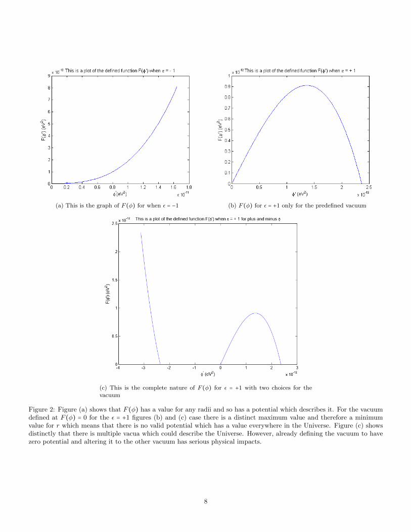
(a) This is the graph of F (φ) for when ε = −1 (b) F (φ) for ε = +1 only for the predefined vacuum

(c) This is the complete nature of F (φ) for ε = +1 with two choices for thevacuum

Figure 2: Figure (a) shows that F (φ) has a value for any radii and so has a potential which describes it. For the vacuumdefined at F (φ) = 0 for the ε = +1 figures (b) and (c) case there is a distinct maximum value and therefore a minimumvalue for r which means that there is no valid potential which has a value everywhere in the Universe. Figure (c) showsdistinctly that there is multiple vacua which could describe the Universe. However, already defining the vacuum to havezero potential and altering it to the other vacuum has serious physical impacts.

8

Figure 3: A graph which shows the force of the new canonical scalar potential with a non-linear kinetic screening term (red

line). The non-linear term changes the evolution of the force and causes it to vary as r−23 (blue line)at short distances and

a 1r2

(green line) dependence similar to the Newtonian Force at large distance. This shows how the screening mechanismaffects the dynamics of the system

5.2.2 Calculation of the Potential

As the effects of a point source outside the almost point source are more concerning than within the source, only r > ηwill be considered

For large r, φ′ can be integrated to the following

φ = − αM

16πMPL

1

r+D. (45)

Just as before D is an arbitrary constant which will be set to zero in order for the potential to be zero at infinity. Thereforethe total potential at a large r approximation is therefore;

VT = VN(1 + α). (46)

For small r, integration of equation (41) gives the following,

φ = −3(CΛ4

16π)

13

r13 +D′. (47)

Continuity arguments between equations (45) and (46) can provide an approximate value for D′. There should becontinuity at the Vainshtein Radius rV ,due to its definition,

rV = ( αM

4πMPL)

12 1

Λ(48)

which was defined as the radius of the Oort cloud. At this radius the small and large r approximation are by definitionapproximately equivalent (see equation (42)). Substitution of Λ (using equation (44)) and equating equations (45) and(46) gives the following value for the constant.

D′ = 1.4( αM

8πMPL) 1

rV(49)

9

Following this definition, the potential from the field is

φ = −3( αMΛ4

32πMPL)

13

r13 + 1.4( αM

8πMPL) 1

rV. (50)

The proportionality constants of the new potential and the Newtonian Gravitational can be numerically calculated.Therefore a comparison between the two will ensure that the Cubic Galileon Potential is indeed less than the Newtonianpotential. This explicitly shows that the newly formed potential is much less than the Newtonian Gravitation at radiuswithin the solar system and is of significant value outside the solar system, hence upholding General Relativity. Thereforeusing a value ε = −1 provides a valid continuous solution to the equations of motion. However, naturally arising fromQuantum Field Theory is that ε = +1.

5.3 The Case of ε = +1

From Figure (2) it appears F (φ′) can undergo the same approximation as when ε = −1 for large r and it can. This canbe seen from the equation of motion (37). Applying the same procedure as above, it can be shown that in the r > rVapproximation the force of the field is:

φ′ = αM

8πMPL

1

r2(51)

Moreover, the small r limit has the same equation for the force as the ε = −1 but instead with a minus sign:

φ′

≈ ( −αMΛ4

32πMPL)

13

r−23 (52)

Furthermore, from figure (2) it is indicated that F (φ′) must indeed have a maximum value. The value of φ′ can thenbe calculated using the usual procedure of taking the derivative. From this the maximum φ′ is found to be:

φ′ = 3√

2Λ2 (53)

Substitution of this into the large r approximation above (equation (52)) leads to a value of the radius that is a minimumvalue;

r = ( αM

16√

3πMPL

)12 1

Λ= 1

2 4√

3rV (54)

Below this radius there are no valid solutions to the equations of the motion for the field. Mathematically this is due tothis value being an algebraic branch point, where the roots of equation (37) cancel due to the anti parity symmetry ofthe function. This shows the problematic nature of the naturalness of ε = +1. This issue continues into the next screeningmechanism: The Cubic Galileon.

6 The Cubic Galileon

6.1 Equation of Motion and its Solutions

Instead of introducing a non-linear kinetic term, there is a vast choice of terms which could be added to account for thescreening mechanism. Once such term creates the following Lagrangian under spherical and time symmetry:

S[φ] = ∫ dr 4πr2 [1

2φ′2 + ε

Λ4

φ′2

r2(r2φ′)

′

+ α2

φ

MplT (r)]

[9]

. (55)

The is known as the Cubic Galileon Action. It is given the name Galileon due to its symmetric change in Galilean Shifts.The second term can be differentiated into two terms in order to attain an explicit second differential with respect to φ.The equations of motion of such an action can be solved using the Euler Lagrange equation (24) and doing so providesthe following result,

4πr2α

2

T (r)Mpl

− d

dr[4πr2 (−φ′ + 4ε

Λ3rφ′2)] = 0. (56)

10

Focusing on the vacuum, as the effects on the orbits of planets is due to the value of the potential outside the sun, allowsfor T (r) = 0 hence reducing the equation of motion down further. Integration of both sides therefore leads to the finaldefinition of the equation of motion

φ′ − 4ε

Λ3rφ′2 = C

4πr2= F (φ). (57)

The exact same argument applies as in the General K-Essence case that F (φ′) is small for large r which causes the linearregime to dominate as can be seen on figure (4). The non-linear parts dependence on r has no affect on the approximationsof the large r. Using the argument that as limr→∞ φ′(r) has no screening term the constant C is again as equation (23).This information provides a large r approximation which is the same as the two previous cases of

φ′

≈ αM

8πMPL

1

r2. (58)

The small r on the other hand is significantly different. As can be seen by figure (4) the non-linear term dominates atsmall r due to F (φ′) being large at large r. Neglecting the linear term to approximate φ′ the equation of motion becomes.

φ′ ≈ (− Λ3αM

24επMpl)

12 1√

r(59)

Where the positive root is taken for reasons later explained. It should be noted that physically the force should be real asit describes a measurable entity. Therefore φ′ (remembering φ′ describes the strength the force applied to a unit test massat a position r) should also be real. So the constant within the root must be positive for this to be true and it is true forthe unnatural ε = −1 case. Further inspection shows there is no solution after a specific radius (which will be calculatedlater) as with the previous case for ε = +1. Similar arguments still apply i.e. F (φ) can not be negative and the vacuum(limr→∞) has to be asymptotically reached therefore specific solutions of F (φ) cannot switch between specific vacuums.phi′ can not have a discontinuity and hence the value of F (φ) cannot undergo a sudden change in sign in this case. ε = +1has no valid solution of φ′.

Figure 4: The Cubic Galileon dynamics are very similar to that of the General K-essence. The screening mechanism isinitiated so that the non-linear Galileon term is dominate at small radii (below the Vainsthein radius) so the force goesas 1√r. At large radii it is again comparable to the Newtonian force and goes as 1

r2

11

We can also provide an exact more complex solution using the quadratic formula which gives the following results:

φ′ = Λ3r

8ε

⎛⎝

1 ± [1 − 2εαM

πΛ3Mpl

1

r3]

12 ⎞⎠. (60)

The asymptotic argument and the argument that the solution must cover the entire real positive domain of position impliesagain that ε = −1. Again, as in the previous case of General K-Essence, from the derivation of the Lagrangian it is foundthat the value is once more ε = +1.

6.2 Calculating an Appropriate value of Λ

As before, the screening mechanism needs to be initiated at the radius of the solar system and below. Equation (53) showsthat φ′ at small radii has a lower strength than the Gravitational force on a unit mass if r is small. Therefore the CubicLagrangian provides a screening mechanism. The ratio of the two terms on the left hand side of the equation of motiongives an indication of when the linear term dominates and hence when r is large.

φ′

(4φ′2

Λ3r)∼ 1 (61)

Rearrangement to gain an equation of φ′ and substitution of that equation into the large r approximation and rearrangingonce more finds following equation of Λ,

Λ = ( αM

2Mplπ)

13 1

r= 2.8 × 10−5m = 5.4 × 10−12eV, (62)

when substituting in the appropriate constants (M = Mass of the sun and r = radius of the solar system).

6.3 The Maximum Value of r when ε = +1

The derivative of F (φ′) can be taken and the value of φ′ can be calculated using the usual methods to give following value

of φ′ = Λ3

8r. Substitution into the non-linear approximation, as this is the regime where the maximum lies, leads to the

following result for the maximum value of the radius for which the theory has a solution

r = ( Mα

πMpl)

13 1

Λ(63)

Therefore the equations of motion have no valid solution of φ′ after this radius making it not a useful theory.

6.4 Calculating the Potential for r > ν

The potential φ is the integral of φ′ so the potential when setting the arbitrary coefficient to zero in order for the(limr→∞ φ = 0 is:

φ ≈ − αM

8πMpl

1

r, (64)

which, as required, is the same as the non screened case.For the small r approximation, integration of equation (60) and using continuity at the Vainshtein radius rv leads to

the following potential approximation:

φ ≈ 2( Λ3αM

24πMpl)√r − 3

√4( αM

8πMpl)

23

Λ(1 − 1√3) , (65)

where Λ has been substituted in for rv. Due to the definition of Λ, small radii are radii below the Vainsthein radius.The potential derived varies as

√r. As these are small radii the gravitational potential has a greater strength at every

radii below the Veinsthein radius as it varies as r−1. To check the numerical results, the proportionality constants can besubstituted in and the radii at which the potential dominates could be calculated for the small radii approximation. Itdoes indeed turn out that the Newtonian gravitational force dominates up to the Vainsthein radius.

The Cubic Galileon however is just a specific type of Galileon and, in fact, there are more Galileon actions whichsatisfy Galilean symmetry.

12

7 General Galileon Action

Assuming a Static Universe and Spherical Symmetry the action for a General Galileon is:

S[φ] = ∫ dr 4πr2 [4

∑n=2

Cnφ(r)εn[φ]

Λ3(n−2)+ α

2

φ

MplT (r)]

[9]

(66)

where

εn[φ] =1

r2

d

dr(r4−n (dφ

dr)n−1

) (67)

and the Cn are constants which. With Quantum Field Theory analysis these are C2 = 12, C3 ∼ C4 ∼ O(1). Using Euler

Lagrange equation the following equation of motion can be obtained for the vacuum:

2C2φ′ + 3

rφ′2Λ−3 + 4

r2φ′3Λ−6 = C

4πr2. (68)

7.1 Using the Field Theory Analysis

Figure 5: The General Galileon varies quite significantly to the other two cases. At small radii the Quartic term dominates(blue line) which is of a constant value. This means that the potential is significantly negligible by comparison to theNewtonian Potential. No approximation is really sufficiently close to the force (pink line) at the Vainshtein radii but atlarge radii the linear approximation which is comparable to the Newtonian Potential dominates. The graph shows thatthe cubic term (black) is almost completely ineffective

The equation of motion becomes (neglecting O(1) constants):

φ′ + 1

rφ′2Λ−3 + 1

r2φ′3Λ−6 = C

4πr2(69)

Firstly, deducing the value of φ′ when each term dominates finds the following equations:

For the Kinetic term (the first term) φ′ ∼ C 1

r2(70)

13

For the Cubic term (the second term) φ′ ∼ (CΛ3)12

1√r

(71)

For the Quartic term (the third term) φ′ ∼ (CΛ6)13 (72)

Such approximations are related to a numerical solution of φ′ which roughly is described by each term when each termdominates. This is shown by figure (5) which graphically shows the dominance of the linear regime at large radii andthe quartic regime at small radii. In between there is real accurate approximation of the combined terms which is inconcordance with the numerical term.

7.1.1 When Each Term Dominates

In order to determine which term within the equation of motion (equation (70)) dominates one must ask a set of questions.It does not matter which question is asked first so long as they are coherent. Firstly, when is the linear term greater thanthe cubic term,

φ′

r2 > φ′3r

Λ3. (73)

In such a regime the equation of motion is assumed to be dominated by the linear term. This assumption is valid and isproved later. Due to this domination, φ′ can be approximated to equation (71) and substitution of equation (74) leads tothe following inequality,

r > C13

Λ. (74)

Therefore, for any distance greater than some yet unknown constant, the linear term dominates over the cubic term.The second question follows the same procedure: when does the linear term dominate over the quartic term? Following

the same method the same answer is found. It is that, for both to be true, the linear term does indeed dominate afterthat specific radius and therefore substitution into the linear approximation (equation (71)) is valid.

The third and final question required is therefore: when does the quartic term dominate over the cubic term. Again,following the same procedure, the following maximum radii is found for quartic term domination over cubic term,

r < C13

Λ. (75)

The opposite questions should also be checked to in order to validate the coherency of the solution.

From the above, the cubic and linear terms do not dominate and the quartic term does up to a radius C13

Λ. Where after

this radius the cubic and quartic terms do not dominate and the linear term does. The three answers to the questions only

have one coherent solution which is that the quartic term dominates up to C13

Λand afterwards the linear term dominates

leaving the cubic term not dominating at all. This can be shown in figure (6) (which is a log plot of figure (5) whichenhances the dependence), where the numerical calculated actual value of φ′ dependence follows initially the quartic termfor it then follows the linear regime.

The domination of the linear term as the limr→∞

means that the linear approximation of φ′ should be equation (31) as

the screening mechanism effect goes to limr→∞

= 0. Therefore the value of C, as before, is equation (23). This therefore

means that the large r approximation for φ′ is:

φ′ ∼ αM

8πMpl

1

r2(76)

and the small r approximation for φ′ is:

φ′ ∼ (αMΛ6

8πMpl)

13

(77)

7.1.2 Calculating a Value of Λ

Due to the above, by taking the ratio of the linear term to the quartic term gives an indication of approximately whenthe non-linear term is about to dominate and screening is initiated,

φ′

( φ′3

r2Λ6)∼ 1 (78)

14

Figure 6: The log plot of figure (5) makes it even clearer that the Cubic term never dominates as shown by the analysiswithin the section.

Substitution into the linear approximation (equation (71)) is still a good approximation up to this characteristic screeningradii. This leads to the following value of Λ being (imputing constants as before with M the mass of the sun and α = 1)

Λ = ( αM

8πMpl)

13 1

r= 1.7 × 10−5m−1 = 3.36 × 10−12eV (79)

for the characteristic screening radius to be the size of the solar system as before.

7.1.3 Calculating the Potential

Knowing the large and small radii approximation for φ′ means equations (71) and (73) respectively can be integrated togive the following value of the potential. At large radii the potential is approximately

φ = − αM

8πMpl

1

r. (80)

Where the integration constant is equal to zero as before by requiring that limr→∞

φ = 0. The integration of the small

approximation then gives,

φ = ( αM

8πMpl)

13

r +C ′, (81)

where C ′ is an integration constant. It is not a requirement that these be continuous at the Vainshtein radius, however,during the calculation the negligible effects of the cubic term have be disregarded and therefore a valid approximation

C ′ can be obtained by equating the two approximations at the Vainsthein radius r = ( αM8πMpl

)13 1

Λ. This then sets C ′ =

−2 ( αM8πMpl

)23

Λ and therefore

φ = ( αM

8πMpl)

13

r − 2( αM

8πMpl)

23

Λ (82)

15

7.2 Hierarchies

A further investigation could be in the form of hierarchies by introducing new values for the constants C2 = 12, C3 ∼ C4 ∼

O(1). This could significantly alter the parameter of Λ and also the dominating term at specific radii. It is not so farfor the imagination can concoct such constants that would produce multiple Vainsthein radii of potentially radical values.However, as of yet theory, predicts the above analysis and setting up such hierarchies is probably more of a mathematicalinterest than a physical one as such hierarchies are not particularly natural.

8 Conclusion

Since the 1980’s there has been a need to explain why the universe is accelerating. A possible solution may arise from theuse of screening mechanisms which have a broad range of variety. Dynamically they can be used to introduce a scalar fieldwhich is a solution for an accelerating universe. They even do it without destroying the beauty of General Relativity’sability to predict the keplerian orbits of the planets around our solar system. However, predictions from quantum fieldtheory always suggest the equations of motions have no solution that satisfies a general expression for all radii. Howeverthere are many more theories for screening mechanisms than the few described above all of which vary. It is thereforeperceivable that a break through can be made. Perhaps in the future test of General Relativity within cosmological scalescould provide evidence for the existence of a fifth force which is screened at small distance.

A Appendix

Detailed derivation of the quantum vacuum energy density is as follows. Firstly ,there is a requirement for a few definitions:The conical momentum for a scalar field is defined as

π(x) = ∂L∂φ

(83)

and using this the Hamiltonian density can be formalised,

H = πiφi(x) −L(x). (84)

Just as in the Lagrangian density, the Hamiltonian is related to the Hamiltonian density as follows:

H = ∫ d3x H (85)

In this definition it could be thought as classically that the Hamiltonian describes the entire energy of the field at allpoints in space.

From section 2.2 it was said that a free field coupled to matter could be described as a harmonic oscillator withfrequency ωp =

√p2 +m2 and so φ is a solution to the harmonic oscillator. In addition, any solution to a harmonic

oscillator can be written as a superposition of the raising a† and lower a operators which are defined in Quantum FieldTheory as

a† =√ω

2φ − i√

2ωπ (86)

a =√ω

2φ + i√

2ωπ (87)

These are analogous to the quantum raising and lowering operators for particles. They arise due their nature .They canact on a energy state of the Hamiltonian to raise or lower the energy state and so all possible states can be calculated fromthem. Inversion of equations (89) and (90) shows the superposition for the scalar and its canonical momentum explicitly.Finally taking the Fourier transform (as shown in equation (9) ) gives the following definitions:

φ(x) = 1

(2π)3 ∫ d3p1

2ωp

[apeip⋅x + a†pe

−ip⋅x] (88)

π(x) = −i(2π)3 ∫ d3p

ωp

2[apeip⋅x + a†

pe−ip⋅x] (89)

16

The Hamiltonian which provides an equation of motion for a free particle coupled to matter could be of the form

H = 1

2∫ d3x π2 + (∇φ)2 +m2φ2. (90)

With the substitution of equations (89) and (90) remembering that integration with respect to the field is only for thebasis i.e if their is multiple field terms in a term in the Hamiltonian then their integral are separate. Hence one will bedefined with the momentum p whilst the other will be defined q. Furthermore, using the definition of the delta function;

δ3(p ± q) = 1

(2π)3 ∫∞

−∞

eix⋅(p±q)d3x (91)

will give a Hamiltonian which is dependent on δ3(p + q) and δ3(p − q) on separate terms. Then for each term the deltafunction can be used again in the form

∫ d3q f(q)δ3(p ± q) = f(±p) (92)

therefore changing all q values to p and in doing so making all the exponential terms be equal to one. Also, there is acancellation, due to the definition of ωp, only leaving the Hamiltonian to become

H = 1

2∫

d3p

(2π)3ωp [apa†

p + a†pap] . (93)

This can be simplified further using the following commutation relation which is one of the requirements for canonicalquantisation,

[φ(x), π(y)] = iδ3(x − y) (94)

Which after substitution of values of φ and π which are derived from the rearrangement of terms in equations (87) and(88) and equating the two gives,

[ap, a†p] = (2π)3δ3(p − q). (95)

Due to previous substitutions of the delta function p = q for any function of q and there fore the delta function oncesubstituted into the Hamiltonian becomes δ3(0) and so the Hamiltonian becomes

H = ∫d3p

(2π)3ωp [a†

pap +1

2(2π)3δ3(0)] . (96)

Now with quantisation of field, just like in the simple harmonic oscillator, the ground state ∣0⟩ (defined as ap ∣0⟩ = 0)has a finite energy. Using the Hamiltonian and the definition of the ground state, an eigenvalue can be calculated for thisfinite energy;

H ∣0⟩ = E0 ∣0⟩ = [∫ d3p1

2ωpδ

3(0)] ∣0⟩ . (97)

Using the Fourier Transform definition of the delta function and using boundary conditions that the volume of the universeis the integral over its dimensions in the limit of the size of the sides of the box being infinity i.e.

δ3(0) = 1

(2π)3 ∫∞

−∞

eix⋅(0)d3x = limL→∞

1

(2π)3 ∫L/2

−L/2d3x = V

(2π)3, (98)

the energy density can be calculated in order to prevent an infinite value for the total energy.

ε0 =E0

V= 1

(2π)3 ∫ d3p1

2ωp (99)

There is, however, an ultra-violet divergence therefore a cut-off is required. This cut-off parametrises the validity of thetheory at specific energies. Past this point the theory breaks down and no longer is a good approximation to the realnature of the problem. For the standard model, the theory has been valid up 1TeV . Furthermore, the energy density isonly dependent on the square magnitude of the momentum. Hence the integral is symmetric around the origin in polarcoordinates. Therefore the energy density integral becomes:

ε0 =1

(2π)3 ∫ΛUV

0d3p

1

2ωp = ∫

ΛUV

0dp p2

√p2 +m2 = Λ4

UV (100)

This implies a Cosmological constant of 10−60 which is of order 10−60 different from the observed value.

17

References

[1] Anne Green, 2015, Introduction to Cosmology, Lecture Notes from the University of Nottingham

[2] Bradley W.Carroll, Dale A.Ostile, An Introduction to Modern Astrophysics, 2nd Edition, Pearson PP.186 -189

[3] S. Perlmutter, Measurement of Ω and Λ from 42 High-Redshift Supernovae arXiv:astro-ph/9812133 , (1998)

[4] Svend Erik Rugh, Henrik Zinkernagel, The Quantum Vacuum and the Cosmological Constant Problem, Studies inHistory and Philosophy of Modern Physics,33, 663-705 arXiv:hep-th/0012253, (2000)

[5] N Straumann ,The mystery of the cosmic vacuum energy density and the accelerated expansion of the Universe,IOPScince, Eur. J. Phys. ,20,419, (1999)

[6] David Tong, 2006, Quantum Field Theory, Lecture Notes from the University of Cambridge

[7] Austin Joyce, Bhuvnesh Jain, Justin Khoury, and Mark Trodden, Beyond the Cosmological Standard Model,arXiv:1407.0059v2, (2014)

[8] 3. Vacuum energy and Lambda, 13th May, http://ned.ipac.caltech.edu/level5/March02/Ratra/Ratra3_2_3.html

[9] Galileon as a local modification of gravity, Alberto Nicolis, Riccardo Rattazzi, and Enrico Trincherini Phys. Rev.D,79,064036, (2009)

[10] C. Armendariz-Picon, V. Mukhanov1 and Paul J. Steinhardt, Essentials of k-Essence, arXiv:astro-ph/0006373, (2000)

18