1

V4: FM MODULATION AND DEMODULATION By Laurence G. Hassebrook September 15, 2017

Table of Contents V4: FM MODULATION AND DEMODULATION .............................................................................................. 1

0. Overview ........................................................................................................................................... 1

1. SYSTEM ARCHITECTURE .................................................................................................................... 2

2. MESSAGE SIGNAL GENERATION ....................................................................................................... 3

2.1 Group Name and Number of Bits ................................................................................................... 4

2.2 Bit Sequence Generation ................................................................................................................ 4

3. FM MODULATION ............................................................................................................................. 4

4. CHANNEL MODEL .............................................................................................................................. 8

5. FM DEMODULATION ....................................................................................................................... 10

6. PERFORMANCE VERIFICATION ........................................................................................................ 14

7. REFERENCES .................................................................................................................................... 16

A. APPENDIX: INSTRUCTOR PROGRAMS ............................................................................................. 16

A.1 BGEN ................................................................................................................................................. 16

A.2 CHANNEL........................................................................................................................................... 16

A.3 BITCHECK .......................................................................................................................................... 18

0. Overview In this visualization we use our MATLAB based communication simulation system. The FM modulation scheme is implemented with the simulation and the student is asked to maximize the number of message bits without receiving an error. Baseline parameter values are given and the modulation and demodulation technique is given mathematically. The student is required to implement the mathematics of the modulator and demodulator to MATLAB code. In this visualization the student only needs to submit their simulation .m files to the instructor. No written report is necessary.

2

The students are also required to formulate a group name, send the instructor their modified createBsize.m, modulator.m and demodulator.m files along with their group member names.

1. SYSTEM ARCHITECTURE The system architecture includes programs that the student modifies and programs that the instructor uses to evaluate their system with. The student has access to the instructor programs so that they can pre-evaluate their systems performance. Given the student programs, the students are required to comply with the File and Data formatting specifications. The student programs have the I/O functionality already built in and specify sections where the students can insert their code. Referring to Figs. 1-1 and 1-2, the procedure for running the system is as follows:

1. (student) Edit in the group name and number of bits (Nbit) into name_createBsize.m and change name to name_createBsize.m.

2. (student) Run name_createBsize.m. This stores Nbit and groupname. 3. (instructor) Edit in group name into Bgenxx.m and run program. This stores two files, one

with the random bit sequence of Nbit bits and the other file contains the active group being processed.

4. (student) Run name_modulator.m. The input is the Message signal is the random bit sequence. The bit sequence is scaled to be bipolar. Using a kronecker product operation, the bipolar message sequence is upsampled to length N. This in turn is modulated using DSBSC modulation at a carrier frequency, kc, specified by the student. The modulator outputs two files, the first with the modulated signal exactly N real elements long and the other a special trinary signal where 1 indicates time location of a “1” bit and -1 indicates the location of a “0” bit. This trinary signal is NOT passed to the demodulator but ONLY ACCESSED by the bitcheckxx.m program.

5. (instructor) Run channelxx.m. The channel filters the spectrum of the modulated signal and adds Gaussian white noise to the signal based on the minimum and maximum values in the signal. The instructor determines the channel transfer function and the amount of noise added. The filtered noisy output is stored in name_r.mat as the real vector “r” that is N elements in length. Channel will also test for errors in the input data format.

6. (student) Run name_demodulator.m. The student may use any parameters used in the modulator, including the number of bits, and will process the input “r” signal vector from the Channel. However, there is NO KNOWLEDGE of the random bit sequence allowed. The output of the demodulator, real vector Bs, is stored in name_Bs.mat.

7. (instructor) Run bitcheckxx.m. Bitcheck uses the Bcheck signal generated in the Modulator to test for 1 or 0 bits. It prints out any errors in format but most importantly how many false alarms and misses occur in the detection process. If there are errors in detection then a figure will be generated revealing the local signal characteristics that led to the error.

3

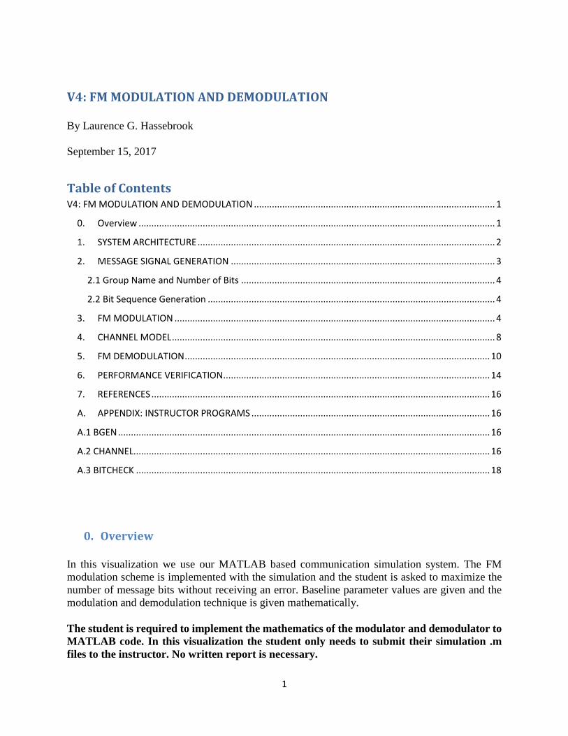
Figure 1-1: Simulation Flow Chart with associated MATLAB programs and data variables and vectors.

The flowchart in Fig. 1-1 shows the relationship of the MATLAB functions with respect to a standard communications system flowchart. Notice that “name_modulator.m” both encodes by upsampling the bit sequence and modulates. The function Bitcheckxx.m both decodes by thresholding the Bs output vector from the demodulator as well as tests for detection errors based on the Bcheck vector.

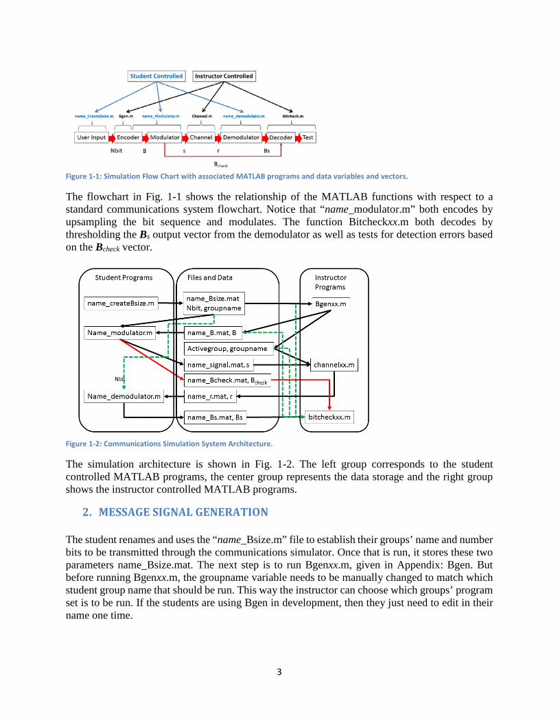
Figure 1-2: Communications Simulation System Architecture.

The simulation architecture is shown in Fig. 1-2. The left group corresponds to the student controlled MATLAB programs, the center group represents the data storage and the right group shows the instructor controlled MATLAB programs.

2. MESSAGE SIGNAL GENERATION The student renames and uses the “name_Bsize.m” file to establish their groups’ name and number bits to be transmitted through the communications simulator. Once that is run, it stores these two parameters name_Bsize.mat. The next step is to run Bgenxx.m, given in Appendix: Bgen. But before running Bgenxx.m, the groupname variable needs to be manually changed to match which student group name that should be run. This way the instructor can choose which groups’ program set is to be run. If the students are using Bgen in development, then they just need to edit in their name one time.

4

2.1 Group Name and Number of Bits Below is the source code for the name_createBsize.m program. For this example, “FM” has been entered as the group name and ???? need to be replaced by a number. For example, replace ???? with 2*2048 which means that 4096 bits will be transmitted through the communication system. % generate groupname_Bsize.mat clear; % INSERT GROUP NAME AND NUMBER OF BITS groupname='FM' % name of group Nbit=??? % END OF INSERT % name of output file that stores Nbit and filename filename=sprintf('%s_Bsize.mat',groupname) save(filename); % stores groupname, Nbit to DSBSC_Bsize.mat

2.2 Bit Sequence Generation From Appendix: Bgen, the only line of code that would need to be changed is groupname='FM' % instructor enters this name to select student project In this case ‘FM’ is entered but should be whatever the group name is. Bgenxx.m generates a pseudo-random set of bits, Nbit long, to be transmitted through the communication system.

3. FM MODULATION The modulator inputs the bit sequence and knows the full number of samples N to be used in the system. It first determines the number of samples, Nsample, per bit. Then using the kronecker product to upsample the bit sequence to the message sequence plus any padding necessary to reach length N. The mathematical representation for this operation is:

( )sNmm ubs ⊗−= 12 (3.1)

where sm is the signal vector, bm is the binary message sequence, ⊗ is the Kronecker product and uNs is a unit vector Ns = Nsample long. % generate bit matrix based on groupname_Bsize.mat clear all; Nshowbits=4; % number of bits to show in figures load 'FM_B.mat'; load 'FM_Bsize.mat'; % generate a real vector s, N=131072*8 or let N be less for debug process N=131072*8 % N is set by instructor and cannot be changed % CREATE THE MESSAGE SIGNAL Nsample=floor(N/Nbit) % form pulse shape pulseshape=ones(1,Nsample);

5

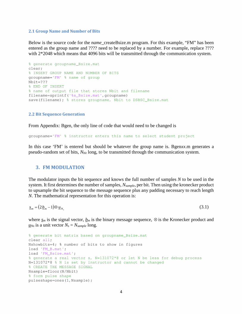
% modulate sequence to either +1 and -1 values b1(1:Nbit)=2*B(1,1:Nbit)-1; stemp=kron(b1,pulseshape); % form continuous time approximation of message sm=-ones(1,N); if N > (Nsample*Nbit) sm(1:(Nsample*Nbit))=stemp(1:(Nsample*Nbit)); else sm=stemp; end; size(sm) % verify shape % plot message signal or a section of the message signal figure(1); if Nbit<(Nshowbits+1) plot(sm); axis([1,N,-1.1,1.1]); xlabel('Message Signal'); else plot(sm(1:(Nsample*Nshowbits))); axis([1,(Nsample*Nshowbits),-1.1,1.1]); xlabel('Sample section of Message Signal'); end; print -djpeg Modulator_figure1

Figure 3-1: Sample section of Message sequence after upsampling.

% FT of message waveform Sm=abs(fftshift(fft(sm))); figure(2); k=0:(N-1); k=k-N/2; plot(k,Sm); xlabel('DFT spectrum of Message Signal'); print -djpeg Modulator_figure2

6

Figure 3-2: Message signal spectra.

The actual modulator code is placed between the commented sections below. The carrier frequency, kc, is in cycles per N samples. Its value should be as high as possible without suffering too much attenuation from the Channel response. If it is attenuated by the channel then the SNR will decrease because the channel noise is proportional to the max-min value before the signal is filtered by the channel. The cutoff for the channel is fc=N/4. So a good first guess of a kc value might be kc=N/8 which is half the channel cutoff. The frequency varies by +/- kdelta from the carrier frequency. For this example we used kdelta =N/64. So if sm(t)=1 then the frequency will be kc + kdelta and if sm(t)= -1 then the frequency will be kc – kdelta. Given the carrier frequency, the FM modulation would be

( ) ( )( )

+= N

tktskts deltamcπ2cos (3.2)

% INSERT MODULATION EQUATION: % INSERT MODULATION EQUATION: % INSERT MODULATION EQUATION: Inputs sm vector, kc, t and N % create AM modulation signal s t=0:(N-1); kc=??? s=???; % use equation 3.2 to write the vector-MATLAB equivalent % END OF MODULATION INSERT % END OF MODULATION INSERT % END OF MODULATION INSERT % plot AM signal figure(3); if Nbit<(Nshowbits+1) plot(s); axis([1,N,-1.1,1.1]); xlabel('FM Signal'); else Ntemp=Nsample*Nshowbits; plot(s(1:Ntemp)); axis([1,Ntemp,-1.1,1.1]); xlabel('Sample section of FM Signal'); end; print -djpeg Modulator_figure3

7

Figure 3-3: Sample section of FM modulated signal.

S=abs(fftshift(fft(s))); figure(4); k=0:(N-1); k=k-N/2; plot(k,S); xlabel('Spectrum of FM Signal'); print -djpeg Modulator_figure4

Figure 3-4: Spectrum of FM modulated Signal.

% create the bit check matrix to only be used by the Bcheckxx.m file % YOU CANNOT PASS THIS INFORMATION TO YOUR DEMODULATOR!! samplepulse=zeros(1,Nsample); samplepulse(floor(Nsample/2))=1; Bcheck=zeros(1,N); % modulate first sequence to either +1 and -1 values b1check(1:Nbit)=2*B(1,1:Nbit)-1; bchecktemp=kron(b1check,samplepulse); Bcheck=zeros(1,N); if N > (Nsample*Nbit) Bcheck(1:(Nsample*Nbit))=bchecktemp(1:(Nsample*Nbit)); else Bcheck=bchecktemp; end;

8

figure(5); if Nbit<(Nshowbits+1) n=1:N; plot(n,sm,n,Bcheck); axis([1,N,-1.1,1.1]); xlabel('Bit Check Signal'); else Ntemp=Nsample*Nshowbits; n=1:Ntemp; plot(n,sm(1:Ntemp),n,(0.9*Bcheck(1:Ntemp))); axis([1,Ntemp,-1.1,1.1]); xlabel('Sample Section of Bit Check Signal'); end; print -djpeg Modulator_figure5 save 'FM_signal' s; save 'FM_Bcheck' Bcheck;

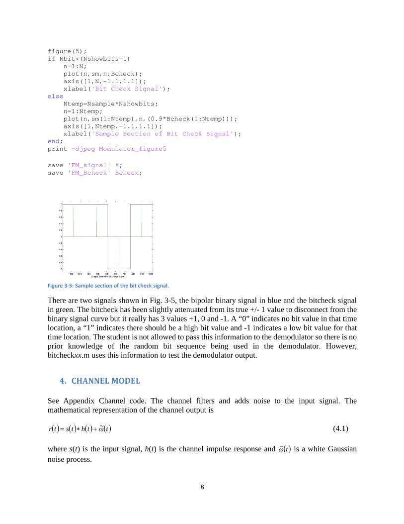
Figure 3-5: Sample section of the bit check signal.

There are two signals shown in Fig. 3-5, the bipolar binary signal in blue and the bitcheck signal in green. The bitcheck has been slightly attenuated from its true +/- 1 value to disconnect from the binary signal curve but it really has 3 values +1, 0 and -1. A “0” indicates no bit value in that time location, a “1” indicates there should be a high bit value and -1 indicates a low bit value for that time location. The student is not allowed to pass this information to the demodulator so there is no prior knowledge of the random bit sequence being used in the demodulator. However, bitcheckxx.m uses this information to test the demodulator output.

4. CHANNEL MODEL See Appendix Channel code. The channel filters and adds noise to the input signal. The mathematical representation of the channel output is

( ) ( ) ( ) ( )tthtstr ω~+∗= (4.1) where s(t) is the input signal, h(t) is the channel impulse response and ( )tω~ is a white Gaussian noise process.

9

Figure 4-1: Log Magnitude Spectrum of input signal.

Fig. 4-1 is obtained by taking the log of the input spectrum such that

( )( )1.0log +fS

Figure 4-2: Channel filter response.

The channel uses a butterworth frequency response as shown in Fig. 4-2.

Figure 4-3: Input response after filtering.

10

Figure 4-4: Sample sequence of original modulated input signal

Figure 4-5: Input signal after channel filtering but no noise has been added.

Figure 4-6: Final output r(t) of channel after filtering and additive noise.

Fig. 4-6 shows the final channel response after filtering and additive noise corruption.

5. FM DEMODULATION The demodulation simulates a balanced frequency discriminator.[1] A simple frequency discriminator is shown in Fig. 5-1. The idea is to design a low pass filter so that the frequency range is within the roll off of the filter centered around its cutoff frequency. This filter attenuates

11

the signal based on its instantaneous frequency. That result is followed by an envelope detector similar to the one used to demodulate AM signals.

Figure 5-1: Simple frequency discriminator.

In the simulation we use a balanced frequency discriminator [1] with full rectification in the envelope detectors as shown in Fig. 5-2.

Figure 5-2: Balanced frequency discriminator.

The balanced frequency discriminator uses two bandpass filters with different center frequencies. The center frequencies correspond to the minimum and maximum signal frequencies. To get the frequency discrimination, each bandpass filter output is envelope detected and then differenced as shown in Fig. 5-2. The mathematics for these is indicated near the question marked lines in the source code below. % generate bit matrix based on groupname_Bsize.mat clear all; Nshowbits=4; load 'FM_Bsize'; % get number of bits sizes load 'FM_r'; [M,N]=size(r) Nsample=floor(N/Nbit) The first thing the demodulator needs to do is create the two bandpass filters for the balanced discrimiantor. The filter center frequencies are based on the two extreme frequencies of the modulator such that

deltacc kkk −=0 (5.1)

12

and

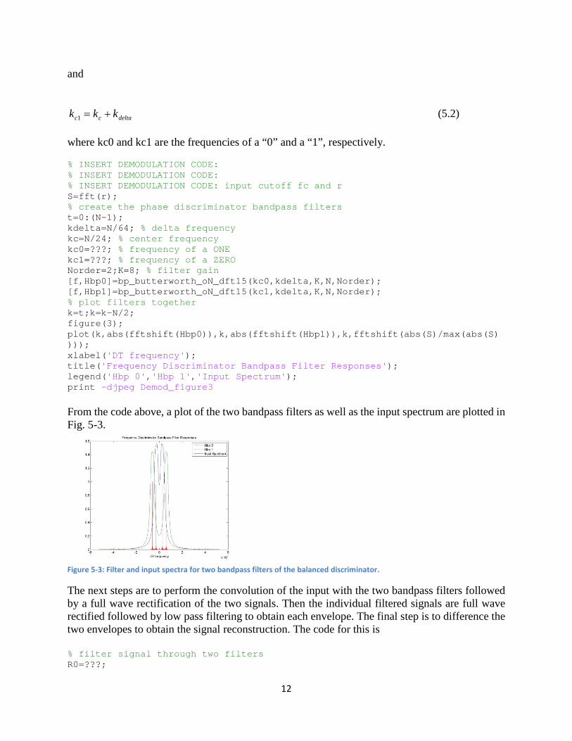
deltacc kkk +=1 (5.2) where kc0 and kc1 are the frequencies of a “0” and a “1”, respectively. % INSERT DEMODULATION CODE: % INSERT DEMODULATION CODE: % INSERT DEMODULATION CODE: input cutoff fc and r S=fft(r); % create the phase discriminator bandpass filters t=0:(N-1); kdelta=N/64; % delta frequency kc=N/24; % center frequency kc0=???; % frequency of a ONE kc1=???; % frequency of a ZERO Norder=2;K=8; % filter gain [f,Hbp0]=bp_butterworth_oN_dft15(kc0,kdelta,K,N,Norder); [f,Hbp1]=bp_butterworth_oN_dft15(kc1,kdelta,K,N,Norder); % plot filters together k=t;k=k-N/2; figure(3); plot(k,abs(fftshift(Hbp0)),k,abs(fftshift(Hbp1)),k,fftshift(abs(S)/max(abs(S)))); xlabel('DT frequency'); title('Frequency Discriminator Bandpass Filter Responses'); legend('Hbp 0','Hbp 1','Input Spectrum'); print -djpeg Demod_figure3 From the code above, a plot of the two bandpass filters as well as the input spectrum are plotted in Fig. 5-3.

Figure 5-3: Filter and input spectra for two bandpass filters of the balanced discriminator.

The next steps are to perform the convolution of the input with the two bandpass filters followed by a full wave rectification of the two signals. Then the individual filtered signals are full wave rectified followed by low pass filtering to obtain each envelope. The final step is to difference the two envelopes to obtain the signal reconstruction. The code for this is % filter signal through two filters R0=???;

13

R1=???; rn0=real(ifft(R0)); rn1=real(ifft(R1)); % rectify the zero and one (use full wave rectification) J=find(rn0<0); rn0(J)=-rn0(J); % full wave rectification of the ZERO signal J=???; rn1(J)=???; % full wave rectification of the ONE signal % create lowpass filter for envelope detection kcE=kc/2 % choose this to be low enough to reduce ripple but high enough

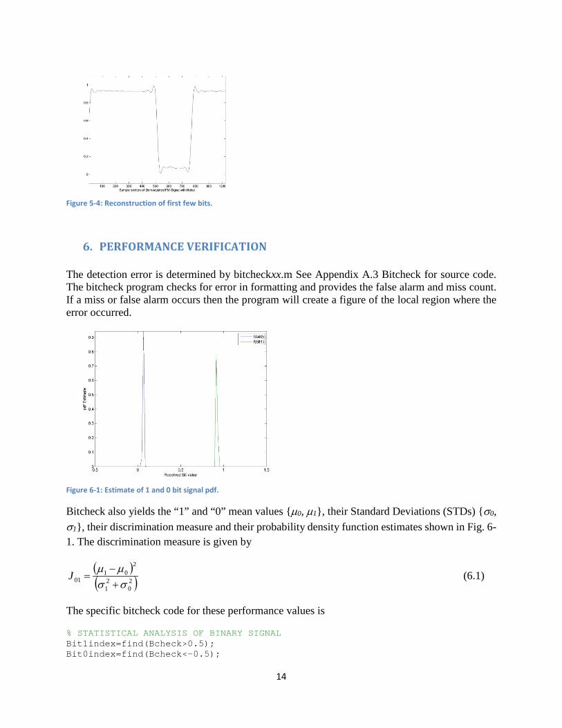
% for bit discrimation Norder=8;K=8; % filter gain [f He]=lp_butterworth_oN_dft15(kcE,K,N,Norder); % rn0=real(ifft(fft(rn0).*He)); % hint for doing the one signal rn1=???; rn=rn1-rn0; % END OF DEMODULATION INSERT: output real vector rn that is N long % END OF DEMODULATION INSERT: % END OF DEMODULATION INSERT: The final step is scaling the signal to be between 0 and 1 for the bit check system. The code for this is % normalize the output to be tested % Bs must be scaled from about 0 to 1 so it can be thresholded at 0.5 by % Bcheck Bs=rn; Bs=Bs-min(Bs); Bs=Bs/max(Bs); save 'FM_Bs' Bs; figure(4) if Nbit<(Nshowbits+1) plot(Bs); axis([1,N,-0.1,1.1]); xlabel('Demodulated FM Signal'); else Ntemp=Nsample*Nshowbits; plot(Bs(1:Ntemp)); axis([1,Ntemp,-0.1,1.1]); xlabel('Sample section of Demodulated FM Signal with Noise'); end; print -djpeg Demod_figure4 A section of bit reconstruction shown in Fig. 5-4.

14

Figure 5-4: Reconstruction of first few bits.

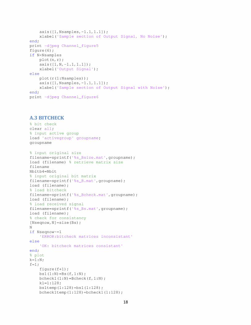
6. PERFORMANCE VERIFICATION The detection error is determined by bitcheckxx.m See Appendix A.3 Bitcheck for source code. The bitcheck program checks for error in formatting and provides the false alarm and miss count. If a miss or false alarm occurs then the program will create a figure of the local region where the error occurred.

Figure 6-1: Estimate of 1 and 0 bit signal pdf.

Bitcheck also yields the “1” and “0” mean values {µ0, µ1}, their Standard Deviations (STDs) {σ0, σ1}, their discrimination measure and their probability density function estimates shown in Fig. 6-1. The discrimination measure is given by

( )( )2

021

201

01 σσµµ

+−

=J (6.1)

The specific bitcheck code for these performance values is

% STATISTICAL ANALYSIS OF BINARY SIGNAL Bit1index=find(Bcheck>0.5); Bit0index=find(Bcheck<-0.5);

15

[MBit1 NBit1]=size(Bit1index); [MBit0 NBit0]=size(Bit0index); Bits1=zeros(1,NBit1); Bits0=zeros(1,NBit0); Bits1=Bs(Bit1index); Bits0=Bs(Bit0index); mu1=mean(Bits1,2) mu0=mean(Bits0,2) var1=var(Bits1); var0=var(Bits0); STD1=sqrt(var1) STD0=sqrt(var0) SQRTofSNR1=mu1/STD1 SQRTofSNR0=mu0/STD0 Discriminate=abs(mu1-mu0)/sqrt(var0+var1) The pdf estimation is performed by the following histogram operations: % HISTOGRAM OF BITS W=100; w=1:W; maxhist=1.5; minhist=-.5; % find coefficients to map from the received values to the histogram index % W=a*maxhist+b, 1=a*minhist+b, a=(W-1)/(maxhist-minhist) b=1-a*minhist acoef=(W-1)/(maxhist-minhist);bcoef=1-acoef*minhist; h1=zeros(1,W); for n=1:NBit1 m=floor(acoef*Bits1(n)+bcoef); if m>0 if m<(W+1) h1(m)=h1(m)+1; end; end; % if m>0 end; % for n h1=h1/NBit1; h0=zeros(1,W); for n=1:NBit0 m=floor(acoef*Bits0(n)+bcoef); if m>0 if m<(W+1) h0(m)=h0(m)+1; end; end; % if m>0 end; % for n h0=h0/NBit0; maxhisto=max(h0); if maxhisto<max(h1) maxhisto=max(h1); end; figure(1); v=(w-bcoef)/acoef; % make horizontal axis be minhist to maxhist units plot(v,h0,v,h1); xlabel('Received Bit value'); ylabel('pdf Estimate'); axis([minhist maxhist 0 maxhisto]);

16

legend('f(bit0)','f(bit1)'); print -djpeg Bitcheck_figure1

7. REFERENCES

1. Principles of Communications, Systems, Modulation, and Noise by R, E. Ziemer and W. H. Tranter, 6th Edition.

A. APPENDIX: INSTRUCTOR PROGRAMS There are 3 instructor controlled programs, Bgenxx.m, Channelxx.m and bitcheckxx.m. The “xx” will be different for different years or visualizations or projects. These programs are in sections A.1, A.2 and A.3 respectively.

A.1 BGEN % generate bit matrix based on groupname_Bsize.mat clear all; groupname='FM' % instructor enters this name to select student project filename=sprintf('%s_Bsize.mat',groupname); load (filename) % retrieve data filename Nbit B=rand(1,Nbit); % generate uniformly distributed random sequence B=binarize(B); % threshold sequence into 0s and 1s size(B) filename=sprintf('%s_B.mat',groupname); save(filename); % save the random bit sequence B % save the active groupname save 'activegroup' groupname;

A.2 CHANNEL % channel function clear all; noiseCoef=0.02 % input active group load 'activegroup' groupname; groupname % input groupname_signal.mat filename=sprintf('%s_signal.mat',groupname); load(filename); % make sure s is real signal=real(s); [M,N]=size(signal) if N~= 1048576 'Incorrect vector length, should be 1048576'

17

end; % % form filter fc=N/4; Norder=6; n=1:N; K=1; % filter gain % low pass filter [f HLP]=lp_butterworth_oN_dft15(fc,K,N,Norder); % filter signal through channel S=fft(signal); H=HLP; R=S.*H; sn=real(ifft(R)); k=n;k=k-N/2; figure(1); plot(k,log(abs(fftshift(S))+.1)); xlabel('Log Magnitude Spectrum of Input Signal'); print -djpeg Channel_figure1 figure(2); plot(k,abs(fftshift(H))); axis([k(1),k(N),-.1, 1.1]); xlabel('Spectrum of Channel'); print -djpeg Channel_figure2 figure(3); plot(k,fftshift(log(abs(R)+.1))); xlabel('Log Spectrum of Output Signal, No Noise'); print -djpeg Channel_figure3 % find noise deviation sigma=noiseCoef*(max(signal)-min(signal)) % add noise w=sigma*randn(1,N); r=sn+w; % store result in groupname_r.mat filename=sprintf('%s_r.mat',groupname); save(filename,'r'); % PLOT spectrum and sample sections of the signal figure(4); Nsamplesection=20; Nsamples=floor(N/Nsamplesection); if N<Nsamples plot(n,signal); axis([1,N,-1.1,1.1]); xlabel('Input Signal'); else plot(signal(1:Nsamples)); axis([1,Nsamples,-1.1,1.1]); xlabel('Sample section of Input Signal'); end; print -djpeg Channel_figure4 figure(5); if N<Nsamples plot(n,sn); axis([1,N,-1.1,1.1]); xlabel('Output Signal, No Noise'); else plot(sn(1:Nsamples));

18

axis([1,Nsamples,-1.1,1.1]); xlabel('Sample section of Output Signal, No Noise'); end; print -djpeg Channel_figure5 figure(6); if N<Nsamples plot(n,r); axis([1,N,-1.1,1.1]); xlabel('Output Signal'); else plot(r(1:Nsamples)); axis([1,Nsamples,-1.1,1.1]); xlabel('Sample section of Output Signal with Noise'); end; print -djpeg Channel_figure6

A.3 BITCHECK % bit check clear all; % input active group load 'activegroup' groupname; groupname % input original size filename=sprintf('%s_Bsize.mat',groupname); load (filename) % retrieve matrix size filename Nbitb4=Nbit % input original bit matrix filename=sprintf('%s_B.mat',groupname); load (filename); % load bitcheck filename=sprintf('%s_Bcheck.mat',groupname); load (filename); % load received signal filename=sprintf('%s_Bs.mat',groupname); load (filename); % check for consistancy [Nseqnow,N]=size(Bs); N if Nseqnow~=1 'ERROR:bitcheck matrices inconsistant' else 'OK: bitcheck matrices consistant' end; % plot k=1:N; f=1; figure(f+1); bs1(1:N)=Bs(f,1:N); bcheck1(1:N)=Bcheck(f,1:N); k1=1:128; bs1temp(1:128)=bs1(1:128); bcheck1temp(1:128)=bcheck1(1:128);

19

plot(k1,bs1temp,k1,bcheck1temp); axis([1 128 -0.1 1.1]); xlabel('first few samples of signal'); % loop through bits Btest=zeros(1,Nbit); miss=0; false=0; Nerror=0; nbreceived=0; m=1; nb=1; for n=1:N if Bcheck(m,n) > 0.5 % "1" should be present in check signal if Bs(m,n)>0.5 Btest(m,nb)=1; else 'ERROR, missing 1' 'Bcheck' Bcheck(m,n) 'Bs' Bs(m,n) m n nb if Nerror<10 figure(2+1+Nerror); istart=n-(2*N/Nbit); istop=n+(2*N/Nbit); if istart<1 istart=1 end; if istop>N istop=N end; clear x; x=1:(1+istop-istart); btemp=x; bchecktemp=x; btemp(1:(1+istop-istart))=Bs(m,istart:istop); bchecktemp(1:(1+istop-istart))=Bcheck(m,istart:istop); plot(x,btemp,x,bchecktemp); %clear x,btemp,bchecktemp; end; miss=miss+1; Nerror=Nerror+1; end; nb=nb+1; nbreceived=nbreceived+1; end; if Bcheck(m,n) < -0.5 % "-1" should be present in check signal if Bs(m,n) < 0.5 % "0" is present demodulated/binarized signal Btest(m,nb)=0; else 'ERROR, missing 0' 'Bcheck' Bcheck(m,n) 'Bs'

20

Bs(m,n) m n nb if Nerror<10 figure(2+1+Nerror); istart=n-(2*N/Nbit); istop=n+(2*N/Nbit); if istart<1 istart=1 end; if istop>N istop=N end; clear x; x=1:(1+istop-istart); btemp=x; bchecktemp=btemp; btemp(1:(1+istop-istart))=Bs(m,istart:istop); bchecktemp(1:(1+istop-istart))=Bcheck(m,istart:istop); istart istop size(x) size(btemp) size(bchecktemp) plot(x,btemp,x,bchecktemp); end; false=false+1; Nerror=Nerror+1; end; nb=nb+1; nbreceived=nbreceived+1; end; end; nbsent=Nbit nbreceived miss false Nerror if nbsent~=nbreceived 'Error between sent and recieved' 'Number of ones and zeros sent' Nones=sum(sum(B)) Nzeros=nbsent-Nones end; % STATISTICAL ANALYSIS OF BINARY SIGNAL Bit1index=find(Bcheck>0.5); Bit0index=find(Bcheck<-0.5); [MBit1 NBit1]=size(Bit1index); [MBit0 NBit0]=size(Bit0index); Bits1=zeros(1,NBit1); Bits0=zeros(1,NBit0); Bits1=Bs(Bit1index); Bits0=Bs(Bit0index); mu1=mean(Bits1,2) mu0=mean(Bits0,2) var1=var(Bits1);

21

var0=var(Bits0); STD1=sqrt(var1) STD0=sqrt(var0) SQRTofSNR1=mu1/STD1 SQRTofSNR0=mu0/STD0 Discriminate=abs(mu1-mu0)/sqrt(var0+var1) % HISTOGRAM OF BITS W=100; w=1:W; maxhist=1.5; minhist=-.5; % find coefficients to map from the received values to the histogram index % W=a*maxhist+b, 1=a*minhist+b, a=(W-1)/(maxhist-minhist) b=1-a*minhist acoef=(W-1)/(maxhist-minhist);bcoef=1-acoef*minhist; h1=zeros(1,W); for n=1:NBit1 m=floor(acoef*Bits1(n)+bcoef); if m>0 if m<(W+1) h1(m)=h1(m)+1; end; end; % if m>0 end; % for n h1=h1/NBit1; h0=zeros(1,W); for n=1:NBit0 m=floor(acoef*Bits0(n)+bcoef); if m>0 if m<(W+1) h0(m)=h0(m)+1; end; end; % if m>0 end; % for n h0=h0/NBit0; maxhisto=max(h0); if maxhisto<max(h1) maxhisto=max(h1); end; figure(1); v=(w-bcoef)/acoef; % make horizontal axis be minhist to maxhist units plot(v,h0,v,h1); xlabel('Received Bit value'); ylabel('pdf Estimate'); axis([minhist maxhist 0 maxhisto]); legend('f(bit0)','f(bit1)'); print -djpeg Bitcheck_figure1