QUANTICOLA Quantitative Approach to Management and Design of

Collective and Adaptive Behaviours

quan col. . ...............................http://www.quanticol.eu

D2.1

A preliminary investigation of capturing spatial information forCAS

Revision: 1.0; Mar 31, 2014

Author(s): Vashti Galpin (UEDIN), Luca Bortolussi (CNR), Vincenzo Ciancia (CNR),Allan Clark (UEDIN), Rocco De Nicola (IMT), Cheng Feng (UEDIN), Stephen Gilmore(UEDIN), Nicolas Gast (EPFL/Inria), Jane Hillston (UEDIN), Alberto Lluch-Lafuente(IMT), Michele Loreti (IMT), Mieke Massink (CNR), Laura Nenzi (IMT), DanielReijsbergen (UEDIN), Valerio Senni (IMT), Francesco Tiezzi (IMT), Mirco Tribastone(SOTON), Max Tschaikowski (SOTON)

Due date of deliverable: Month 12 (March 2014)

Actual submission date: Mar 31, 2014

Nature: R. Dissemination level: PU

Funding Scheme: Small or medium scale focused research project (STREP)

Topic: ICT-2011 9.10: FET-Proactive ‘Fundamentals of Collective Adaptive Systems’ (FOCAS)

Project number: 600708

Coordinator: Jane Hillston (UEDIN)

e-mail: Jane.Hillston@ed.ac.uk

Fax: +44 131 651 1426

Part. no. Participant organisation name Acronym Country1 (Coord.) University of Edinburgh UEDIN UK2 Consiglio Nazionale delle Ricerche – Istituto di Scienza e Tecnologie

della Informazione “A. Faedo”CNR Italy

3 Ludwig-Maximilians-Universitat Munchen LMU Germany4 Ecole Polytechnique Federale de Lausanne EPFL Switzerland5 IMT Lucca IMT Italy6 University of Southampton SOTON UK7 Institut National de Recherche en Informatique et en Automatique INRIA France

An investigation of capturing spatial information (Revision: 1.0; Mar 31, 2014) Mar 31, 2014

Executive summary

Space is important in the QUANTICOL project because the project case studies includesmart transport, and quantitative modelling of transport has inherent spatial aspects. Thisdeliverable presents a review of the literature about spatial modelling within and beyondcomputer science, and a classification of the different approaches reviewed. The objectiveof the classification is to make clear what approaches are available and how they differfrom each other. This will be used to guide future work on spatial approaches within theproject. Furthermore, the classification enables the identification of the approaches thathave been used in the initial work on case studies in the realm of smart transport.

This deliverable first identifies the aspects of non-spatial modelling that are importantin the context of the QUANTICOL project. Time can be modelled in a discrete or continu-ous manner. States can be discrete, representing attributes of an individual. For example,when considering bike sharing, inUse (busy), onStand (idle) or atWorkshop (under repair)might be appropriate states for a bike. Alternatively, states can be continuous represent-ing an attribute (for example, seat height). In the case of discrete states, it is possibleto perform aggregation by considering populations, namely how many individuals are ineach state, and to acquire an understanding of the overall behaviour of the population,rather than of individuals. Mean-field techniques can be employed to transform a discretepopulation approach to one that considers continuous populations that approximate thediscrete approach.

To this context, space is introduced. Space can be discrete and described by a graphof locations. Depending on the structure of the graph and the parameters associated withlocations and movement between locations, discrete space can be classified as regular orhomogeneous. Space can be seen as continuous: as Euclidean space in one, two or threedimensions. Space can also be considered abstractly as topological space, whether discreteor continuous and this approach allows for reasoning about concepts such as adjacencyand neighbourhoods.

This deliverable describes the modelling techniques that are currently available forthe different combinations of time, state, aggregation and space, giving both a tabularclassification as well as high-level and formal descriptions of the techniques. For each rep-resentation, examples are given of its use in different disciplines, including ecology, biology,epidemiology and computer science. In particular, the modelling goals are considered forthese techniques, and compared with the goals of the QUANTICOL project. This deliv-erable also has the aim of identifying disparate uses of terminology in various approaches.

Both current and future case studies relevant to the project are classified in termsof how they use time, state, aggregation and space and finally conclusions are presentedtaking into account the literature reviewed, what has been modelled and what the goalsof the project are for modelling of smart transport.

The preliminary guidelines arising from the review and classification are to focus onpatch models and associated techniques although continuous space models of individualsmay be important in certain cases. Items proposed for further research are understandingand developing mean-field techniques, spatial and non-spatial moment closure methodsand hybrid spatial approaches. The document closes with a future work plan for WorkPackage 2.

QUANTICOL 1 Mar 31, 2014

An investigation of capturing spatial information (Revision: 1.0; Mar 31, 2014) Mar 31, 2014

Contents

1 Introduction 3

2 A classification of space and movement modelling techniques 42.1 Notation . . . . . . . . . . . . . . . . . . . . . . . . . . . . . . . . . . . . . . . . . . . . 42.2 Non-spatial modelling dimensions . . . . . . . . . . . . . . . . . . . . . . . . . . . . . . 42.3 Time-based non-spatial modelling techniques . . . . . . . . . . . . . . . . . . . . . . . 62.4 Introducing space . . . . . . . . . . . . . . . . . . . . . . . . . . . . . . . . . . . . . . . 62.5 Spatial modelling techniques . . . . . . . . . . . . . . . . . . . . . . . . . . . . . . . . 82.6 Movement . . . . . . . . . . . . . . . . . . . . . . . . . . . . . . . . . . . . . . . . . . . 11

2.6.1 Discrete space . . . . . . . . . . . . . . . . . . . . . . . . . . . . . . . . . . . . 122.6.2 Continuous space, no aggregation . . . . . . . . . . . . . . . . . . . . . . . . . . 122.6.3 Continuous space, aggregation . . . . . . . . . . . . . . . . . . . . . . . . . . . 12

2.7 Conclusion . . . . . . . . . . . . . . . . . . . . . . . . . . . . . . . . . . . . . . . . . . 12

3 Discrete space modelling techniques 133.1 Spatial homogeneity . . . . . . . . . . . . . . . . . . . . . . . . . . . . . . . . . . . . . 133.2 Spatial regularity . . . . . . . . . . . . . . . . . . . . . . . . . . . . . . . . . . . . . . . 143.3 Neighbours and neighbourhoods . . . . . . . . . . . . . . . . . . . . . . . . . . . . . . 153.4 Boundary conditions . . . . . . . . . . . . . . . . . . . . . . . . . . . . . . . . . . . . . 153.5 Discrete space without state-based aggregation . . . . . . . . . . . . . . . . . . . . . . 163.6 Discrete space with state-based aggregation . . . . . . . . . . . . . . . . . . . . . . . . 163.7 Examples of existing use . . . . . . . . . . . . . . . . . . . . . . . . . . . . . . . . . . . 17

3.7.1 Ecology . . . . . . . . . . . . . . . . . . . . . . . . . . . . . . . . . . . . . . . . 183.7.2 Biology . . . . . . . . . . . . . . . . . . . . . . . . . . . . . . . . . . . . . . . . 193.7.3 Epidemiology . . . . . . . . . . . . . . . . . . . . . . . . . . . . . . . . . . . . . 193.7.4 Other . . . . . . . . . . . . . . . . . . . . . . . . . . . . . . . . . . . . . . . . . 20

3.8 Application to smart transport case studies . . . . . . . . . . . . . . . . . . . . . . . . 203.8.1 Bus models . . . . . . . . . . . . . . . . . . . . . . . . . . . . . . . . . . . . . . 203.8.2 Bike sharing models . . . . . . . . . . . . . . . . . . . . . . . . . . . . . . . . . 21

4 Continuous space modelling techniques 224.1 Continuous space without state-based aggregation . . . . . . . . . . . . . . . . . . . . 234.2 Continuous space with state-based aggregation . . . . . . . . . . . . . . . . . . . . . . 234.3 Examples of existing use . . . . . . . . . . . . . . . . . . . . . . . . . . . . . . . . . . . 23

4.3.1 Ecology . . . . . . . . . . . . . . . . . . . . . . . . . . . . . . . . . . . . . . . . 244.3.2 Biology . . . . . . . . . . . . . . . . . . . . . . . . . . . . . . . . . . . . . . . . 244.3.3 Epidemiology . . . . . . . . . . . . . . . . . . . . . . . . . . . . . . . . . . . . . 244.3.4 Networking . . . . . . . . . . . . . . . . . . . . . . . . . . . . . . . . . . . . . . 25

4.4 Application to smart transport case studies . . . . . . . . . . . . . . . . . . . . . . . . 25

5 Topological space models 255.1 Examples of existing use . . . . . . . . . . . . . . . . . . . . . . . . . . . . . . . . . . . 265.2 Application to smart transport case studies . . . . . . . . . . . . . . . . . . . . . . . . 27

6 Conclusion 276.1 The classification revisited . . . . . . . . . . . . . . . . . . . . . . . . . . . . . . . . . . 276.2 Conclusions . . . . . . . . . . . . . . . . . . . . . . . . . . . . . . . . . . . . . . . . . . 28

References 30

QUANTICOL 2 Mar 31, 2014

An investigation of capturing spatial information (Revision: 1.0; Mar 31, 2014) Mar 31, 2014

1 Introduction

In the QUANTICOL project, we focus on the quantitative modelling of collective adaptive systems(CAS), looking particularly at smart transport systems such as bus services and bicycle sharing sys-tems. An important aspect of both of these systems is location in and movement through space, andwe wish to include this feature in our models to ensure that our modelling techniques allow for asufficient level of accuracy to achieve our modelling goals. An appropriate starting point is to under-stand how space has been modelled both in the discipline of computer science and in other disciplines.Additionally, modelling of the QUANTICOL case studies is already ongoing using existing modellingtechniques as the project is strongly driven by its domain of application and assessment of the wayspace has been modelled in these examples gives further guidance for how to proceed.

This deliverable presents the results of our investigation into the mathematical modelling tech-niques that have been used to represent space and their match to the objectives of the QUANTICOLproject. Our general approach focusses on the behaviour over time of groups of individual entities, andunderstanding from the possible behaviour of these entities what the overall behaviour of populationsis, considering both stochastic interpretations and deterministic approximations of this time-varyingbehaviour. To investigate the introduction of space into this approach, we have reviewed the literatureto understand the modelling techniques that consider individuals and their populations in space. Toclarify terminology, the terms modelling technique and modelling approach will be used to describe ageneral mathematical method used to construct models, and the term model will be used to describea specific representation of a particular system using a modelling technique or approach. In this de-liverable, we assume that the modelling approaches have associated analysis techniques: either in theform of simulation or mathematical techniques that lead to an analytic result, but we do not describethese techniques here.

This deliverable does not consider modelling languages such as process algebras as that is thefocus of Task 2.2, and process algebraic features for modelling space will be considered in the InternalReport of Task 2.2 (due in month 33, December 2015). The deliverable also does not consider spatialprogramming languages such as Proto [VBU13] and TOTA [MVZ05]. The features of these languageswill be considered later in this work package. Furthermore, this deliverable does not cover costs ofanalysis, transformations, convergence results and abstractions of and between spatial representationsas these will be reported in Deliverable 2.3 (due in month 42, October 2016).

Hence this document reports on what representations are present in the modelling literature,drawing from a number of disciplines, and developing a classification of the techniques involved.These techniques will be described abstractly and concretely, through being related both to examplesin the literature, and to the smart transport case studies that are currently being investigated in theQUANTICOL project. An aim of this document is understanding the goals of the existing techniquesso that they can be compared to the goals of the project and so that preliminary guidelines can beprovided. A secondary aim of the document is to identify disparate uses of terminology for the sametechnique across different disciplines (or the use of the same terms for different techniques) to provideclarification for the spatial modelling aspects of this project. Any review of this type has the potentialto be rather long, and hence a separate technical report has been written [GFH+14] for a discussionof details that are not directly relevant for this higher-level overview document.

This document is organised as follows. First, a high-level classification of space is presented, andsome example modelling techniques discussed. After that there are three chapters, each relating toa different approach to space modelling. In each of these chapters, the techniques are described,examples are given of existing use and there is a discussion of how these approaches can be applied toour smart transport case studies, based on the work already done with respect to these case studies andlooking forward to future work. Finally the document presents conclusions, preliminary guidelines,the relationship of this deliverable to other parts of the project and a work plan.

In terms of authorship, Vashti Galpin has written the bulk of the document with others contributingshort pieces of text and descriptions of their modelling of various case studies.

QUANTICOL 3 Mar 31, 2014

An investigation of capturing spatial information (Revision: 1.0; Mar 31, 2014) Mar 31, 2014

2 A classification of space and movement modelling techniques

This section provides a framework in which to understand the various choices that can be made interms of spatial modelling techniques. There exists a rich literature about these techniques and it isnecessary to understand this before making decisions relating to the spatial aspects of the languagesand their semantics in the QUANTICOL project.

We are interested in modelling the collective behaviour of many individuals using a stochasticapproach (based on Markov chains that are discrete time or continuous time1 and we use mean-fieldtechniques2 to obtain a fluid or deterministic approximation of their behaviour [Kur81]. We startfrom information about how each individual changes state over time, and we are interested in howthis affects the overall behaviour of the system over time, either obtaining an exact stochastic analysisof the system, or a deterministic approximation of its behaviour.

Our specific modelling goals are determined by the case studies in the QUANTICOL project whichare smart transport and smart grids. Choice of modelling technique should be informed by the sortof questions for which answers are required. The requirements section in Deliverable 5.1 [TCG+14]considers some of these questions and others will be revealed as the project continues and propertiesfor verification by spatial model-checking are considered. Furthermore, when existing models of casestudies are discussed in Sections 3.8, 4.4 and 5.2, the goal of each model is identified. We return toconsideration of this issue in the final section of this document.

2.1 Notation

To set the scene, some notation will be useful. For illustrative purposes in this document, we considertwo populations PA and PB. At each point in time, each individual in PA is in exactly one of the statesA1, . . . , An and each individual in PB is in exactly one of the states B1, . . . , Bm. We can consider thepopulations in terms of individuals (we may need a naming convention to be able to refer to eachindividual) or in aggregation by counting the number of individuals in each state. This is calleda state-based aggregation and it provides a view of the number of individuals in a population in aparticular state, for each population and each state allowed for that population. Thus, let NAi(t)refer to the number of individuals in population PA that are in state Ai at time t and let NBj (t) referto the number of individuals in population PB that are in state Bj at time t. These will be calledsubpopulations. The total number of individuals in the two populations at time t can be expressed asNA(t) =

∑ni=1NAi(t) and NB(t) =

∑mj=1NBj (t) respectively. Clearly, these counts are in N (which

includes zero). Furthermore, if no births or deaths are assumed, and an individual must be in one ofthe available states3, then NA(t1) = NA(t2) for all times t1 and t2 and the size of PA is a constantNA; similarly the size of PB is NB.

To complete the notation required for populations, we use XAi(t) ∈ R≥0 to represent a non-negative real-valued description of the population PA which in certain approaches is an approximationto NAi(t) and similarly for XBi(t) ∈ R≥0 for PB.

2.2 Non-spatial modelling dimensions

Before space is considered, there are already a number of choices that lead to different approaches tomodelling dynamic systems in a quantified manner. We now consider the dimensions and the choiceson each dimension as informed by the prior research of members of the project into dynamic modellingof systems [BHLM13]. For example, the time dimension considers how time is treated in different typesof Markov chains. There are other aspects of time such as non-determinism and causality, but theseare not a strong focus of our general modelling approach, and so are not included in the classification.

1See the Appendix of this document for a brief introduction to these concepts and population Markov chains.2See the tutorial [BHLM13] and the references therein for more details of the mean-field approach.3In some models, births and deaths can be included for a fixed size population by introducing a “dead” state. However,

this requires that there is a finite maximum population size.

QUANTICOL 4 Mar 31, 2014

An investigation of capturing spatial information (Revision: 1.0; Mar 31, 2014) Mar 31, 2014

Time discreteAggr none stateState discrete continuous discrete continuous

DTMC LMP population difference equations,(discrete-time (labelled Markov DTMC ordinary differentialMarkov chain) process) equations (ODEs)[Nor98] [Pan09] [BHLM13] [BHLM13, MNS11]

Time continuousAggr none stateState discrete continuous discrete continuous

CTMC CTMP population population(continuous-time (continuous-time CTMC ODEsMarkov chain) Markov process)[Nor98] [DP03] [BHLM13, Kur81] [BHLM13, Kur81]

Figure 1: Classification of mathematical models in terms of time, aggregation and state

Time: Time is usually non-negative, strictly increasing and infinite, and can either be a non-negativereal or integer. In some models, a finite end-point may be used to delimit the period of interest.

discrete: In the context of this research, discrete time is used in those modelling approacheswhere choices are probabilistic. At each clock tick (which could be associated with aninteger if useful for the specific model), each individual chooses probabilistically its nextstate. For example, discrete time Markov chains (DTMCs) use this approach [KS76, Nor98].

continuous: Here, time is continuous and this is captured by the fact that actions such aschanging state have a duration associated with them. In the case of continuous timeMarkov chains (CTMCs), stochasticity is introduced by having random durations that aredrawn from exponential distributions [Nor98].

State: States can be viewed as capturing a quality or attribute of an individual. As described above,an individual is assumed to be in a single state at each point in time4.

discrete: Usually when the states associated with an individual are discrete, there are a finitenumber of them. However, in the case of an attribute like year-of-birth, there may be acountably infinite number of values.

continuous: A continuous-valued state can be interpreted as measurement of some quantityassociated with the individual. An example of this would be temperature or height.

Aggregation: As discussed previously, individuals can be considered separately, or the focus can beon the number of individuals in each state. This is more relevant to discrete state approachesthan continuous state. In the continuous case, aggregation can be described by a function, ordiscretisation can be applied to obtain frequency data.

4An individual could have more than one attribute, and then the individual’s state is multidimensional with a valuefor each attribute. In this case, the individual’s state can be seen as a tuple of values.

QUANTICOL 5 Mar 31, 2014

An investigation of capturing spatial information (Revision: 1.0; Mar 31, 2014) Mar 31, 2014

none: Behaviour of each individual is considered separately.

state-based : The behaviour of groups of individuals is considered by counting the number ofindividuals in each state over time (giving a non-negative integer value), or by havinga non-negative real-valued approximation to this number. This approach appears undera number of different names in the literature including population-based, state frequencydata, numerical vector form, and counting abstraction. The term occupancy measure isused when counts are normalised by the population size.

These possibilities can be expressed in a table, which can then be populated with mathematical mod-elling techniques from the literature. Figure 1 illustrates this and describes the modelling techniquesthat fit each combination of each element of each dimension.

2.3 Time-based non-spatial modelling techniques

An important aspect of our prior research is the application of the mean-field technique where theanalysis of a population CTMC or DTMC can be approximated by an analysis using ordinary differ-ential equations (ODEs) [Kur81, BHLM13]. As the number of states of a Markov chain increases (the“state-space explosion” problem), the analysis of the Markov chain becomes intractable. Modelling alarge number of individuals can lead to a very large Markov chain. This can be mitigated by using apopulation Markov chain where behaviour is considered at a population level rather than at an individ-ual level. The choice of a population Markov chain means we are interested in how many individualsare in each state i, given by NAi , and the states in the Markov chain have the form (NA1 , . . . , NAn).However, for large systems this may still not be sufficient to obtain reasonable analysis times, and anapproximation using ODEs obtained from the population Markov chain can be used. This gives a sys-tem of ODEs for the variables (XA1 , . . . , XAn). This population Markov chain considers non-negativeinteger-valued population counts whereas the ODEs take a fluid approach and population quantitiesare non-negative real values. Considering the modelling techniques in Figure 1 for both discrete timeand continuous time, the Markov chain obtained by considering many individuals (in the first column)can be transformed to a smaller Markov chain (in the third column) which can then be approximatedby ODEs (in the fourth column).

This last transformation uses the mean-field approximation technique which comes originally fromphysics, where it refers to the approach where the movement of an individual particle is consideredin the field generated by other particles rather than trying to solve the more complex problem ofmany particles interacting [CL07, MP12]. In modelling of systems, it has come to mean an approachwhere it is assumed that the number of individuals in a stochastic system becomes very large so thatthe population-level behaviour of the system can be expressed as ODEs which provide an “average”behaviour of the system. Results such as those proved by Kurtz [Kur81] demonstrate that under certainconditions, convergence occurs, namely as the number of individuals tends to infinity, the differencebetween the stochastic trajectories of the subpopulation sizes and the deterministic trajectories ofthe subpopulation sizes tends to zero. Practically, in many cases, good approximations using theODE approach over the stochastic approach can be achieved at relatively low numbers of individuals[TGH12] and there are error bounds on the approximations [DN08].

Markov processes (in the second column) do not fit into this work flow and seem different fromthe other modelling techniques, as they are characterised by a continuous state space (which can alsobe interpreted as any continuous aspect of a model, including space).

2.4 Introducing space

Space can be considered in different ways.

continuous: Here, space is represented by real values in the case of one-dimensional space, pairs ofreal values in the two-dimensional case and triples of real values in the three-dimensional case.

QUANTICOL 6 Mar 31, 2014

An investigation of capturing spatial information (Revision: 1.0; Mar 31, 2014) Mar 31, 2014

It is always (uncountably) infinite but may be bounded in extent. Continuous space used in thisway can be seen as an exact representation of actual physical space.

discrete: Approaches that use discrete space assume a number (usually finite) of distinct locationswhere connectivity between locations is described by an adjacency relation. At each location,there can be multiple individuals, although in some cases, such as cellular automata [Ila01], thismay be restricted to a single individual. A location may be an abstraction or aggregation ofactual space.

topological: This approach to space considers the relationships between points in space and containsno notion of time. It can be applied to both discrete and continuous space. Topological spacesconsider space in an abstract manner using open sets from which concepts of continuity, adja-cency and neighbourhoods are defined. Metric spaces have a notion of distance which is used todefine these concepts.

As before, we introduce notation for the remainder of this document. For the purposes of thissection, we only consider 2-dimensional space when we consider continuous space, either R × R or abounded contiguous subset of R×R. Since this provides a uncountably infinite set of points, the moststraightforward way to refer to each point is by its coordinates (x, y).

In the case of discrete space, we assume a finite (or at most countably infinite) set of points L withsome naming convention. There can be a relationship between points in 2-dimensional continuousspace and locations in discrete space. If there is a partition of continuous space into regions then eachlocation can represent a region in continuous space.

Discrete space also requires notions of adjacency and neighbourhood. In the general case, the setof locations L can be taken as the vertices of a graph, and the connections between locations (theadjacency relation) can be defined as edges in that graph. Then the edges of the graph EL are drawnfrom the subsets of size two of the location set P2(L), so EL ⊆ P2(L). Each edge has the form {l1, l2},and edges of the form {l, l} are permitted. For reasons we describe in Section 3, we have chosen touse an undirected graph which is to be understood as allowing movement or interaction in at leastone direction between the two locations.

By adding restrictions to the general case, subclasses of discrete space can be obtained. Forexample, regular discrete space modelling techniques assume that there is a regularity in defining theneighbours of a location but not necessarily in parameters [DL94b, OS71]. In contrast, homogeneousspace techniques take a different approach and assume full connectivity between all regions (giving acomplete graph) and equality of parameters between locations and at locations [Che81]. Both of theseissues will be discussed in more detail and formality in the section on discrete space (Section 3).

We now address an issue of terminology. The term map will be used to represent a two-dimensionalcontinuous representation of space that is to scale, meaning that the ratio between distances is pre-served. On the other hand, the terms location graph or simply graph will be used to denote a repre-sentation that is not to scale but indicates the connections between locations. In between these two,is the category of topological map which is

“a type of diagram that has been simplified so that only vital information remains andunnecessary detail has been removed. These maps lack scale, and distance and directionare subject to change and variation, but the relationship between points is maintained. Agood example is the tube map of the London Underground.” [Wik13b]

The distinction between a topological map and a graph is that although both represent relationshipsbetween points, the topological map is a continuous deformation of the original map, and it alsois a two-dimensional representation of a graph. A graph is more abstract and has no specific two-dimensional representation. Note that planarity (the lack of overlapping edges when embedded in theplane) is not required for topological maps or graphs. Any topological map can be abstracted to agraph of locations, hence defining discrete space.

QUANTICOL 7 Mar 31, 2014

An investigation of capturing spatial information (Revision: 1.0; Mar 31, 2014) Mar 31, 2014

Time continuousAggr none state and/or spaceState discrete continuous discrete continuous

Spacediscrete

general multiple individuals TDSHA, patch CTMC patch ODEsCTMC PDMP [CLBR09] [CLBR09]

[BP10, Dav93]regular interacting particle foraging model foraging model

system (IPS) [MSH05] [MSH05][DL94b]

homo- bike sharing bike sharinggeneous [FG12] [FG12]

continuous molecular dynamics CTMP spatio-temporal partial differential[CPB08] [DP03] point processes equations (PDES)agents [SBG02] [HLBV94]

Figure 2: Classification of mathematical models in terms of time, aggregation, state and space

A table has been constructed to identify mathematical models for the different combinations oftime, aggregation, state and space (see Figure 2). Here, we have chosen to focus on continuous timemodels; however there are discrete time models of various approaches, for example, some variants ofinteracting particle systems (IPSs) use probabilities [DL94b].

All the models appearing in the table consider changing behaviour over time. Characteristics ofspace may or may not change as time passes5. In the case where there are no changes, space can beconsidered independently of time and represented as a topological space. When there are changes inthe characteristics of space over time, the characteristics of space at a specific point in time can beconsidered topologically.

The next section considers each entry of the table in Figure 2 and illustrates the ideas using aconsistent diagrammatic framework.

2.5 Spatial modelling techniques

The techniques described in this section are mainly continuous time, although some have discrete timeanalogues, as mentioned above.

Discrete space, no aggregation, discrete state: The techniques in this category consider spaceto consist of a (finite) number of locations that have connections between them. The most straight-forward way is to consider these models as graphs with the locations as nodes and the links as edges.This type of model is illustrated in Figure 3(1). Here, and throughout this subsection, we assumeindividuals from the two populations already defined. The first, PA consists of red and white tokens,and has states A1 and A2, using our previously introduced notation. The second, PB consists of blueand white tokens with states B1, B2 and B3. The current state of an individual is indicated on the

5An example of this would be off-peak road closures for the painting of road markings.

QUANTICOL 8 Mar 31, 2014

An investigation of capturing spatial information (Revision: 1.0; Mar 31, 2014) Mar 31, 2014

(1)

A1

A1

B1

B3

A1

B2

B3B3B3

A2

(2)

(3)

A1

A1B1

B3

A1

B2

B3

B3

B3

A2

A1B1

B3

A1

B2

B3

B3

A2

(4)

Figure 3: Discrete space: (1) no aggregation, discrete state; (2) no aggregation, continuous state; (3)aggregation of state, possible aggregation of space, discrete state (4) aggregation of state, possibleaggregation of space, continuous state

top of the token. Note that the four diagrams in Figure 3 represent four single points in time and donot show change over time (and similarly for subsequent diagrams). For two-dimensional and three-dimensional space, the best visualisation method for change over time is video. For one-dimensionalspace, a graph with two axes can be used.

Regular space models in this category have a regular pattern of locations [DL94a, DL94b]. Forexample, the locations could be laid out in the rectangular grid, or a hexagonal tiling. The locationsthat represent space can be placed at the nodes of the regular graphs or in the spaces (faces) createdby the regular graph as shown in Figure 4(1). Some models only allow one individual in each location,such as interacting particle systems (IPSs) [DL94b] and cellular automata (CA) [Ila01], but othersmay allow multiple individuals. There is no aggregation of individuals. In Section 3, regular spacewill be formally defined.

Discrete space, no aggregation, continuous state: These techniques differ from those abovein the fact that the state is continuous. This is indicated by a solid token where the height indicatesthe value of a single continuous state. This is an inherently continuous value rather than the notionof approximation by continuous values described earlier in this section. This could be viewed asa measurement such as strength of radio signal or length of battery life. In Figure 3(2), there isan assumption of at most one individual per node, and two values associated with that individual.Different colours have been used in the diagram to make it clear that the values are continuous.

The major difference between this category and the previous one when regular space is considered isthe fact that instead of having discrete states, there is one or more non-negative real values associatedwith each individual as shown in Figure 4(1).

Discrete space, aggregation, discrete state: These techniques differ from those in the firstcategory above in the fact that there is aggregation [MP12]. This means that instead of each individual

QUANTICOL 9 Mar 31, 2014

An investigation of capturing spatial information (Revision: 1.0; Mar 31, 2014) Mar 31, 2014

(1)

A1A1

A1B1

A2A2

B2

B2

B3A2

(2)

(3)

A1

A1

A1

B1

A2

A2

B2

B2

B3A2

A1

B1

A2

B2

B2B3

A2

A1

(4)

Figure 4: Regular discrete space: (1) no aggregation, discrete state; (2) no aggregation, continuousstate; (3) aggregation of state, possible aggregation of space, discrete state (4) aggregation of state,possible aggregation of space, continuous state

being treated separately, individuals in the same state are considered as populations. This is illustratedin Figure 3(3) by the fact that individual tokens are grouped into stacks at nodes in the network.Figure 4(3) shows the regular space case where populations are aggregated at each location [EE04].

Discrete space, aggregation, continuous state: Here each region or point is associated with ap-proximations to the discrete population approach mentioned in the previous item [MP12], as shown inFigure 3(4). At each node, for each state in each population, there is a real number that approximatesthe number of individuals in that state. This is illustrated in the graph by a column with a real-valuedheight for each state in each population. Note that in Figure 3(4), the lowest node has a non-zero valuefor blue tokens in state B3 although there were none in the CTMC model in Figure 3(3), illustratingthat approximation can occur. The case of regular space [LD96] is illustrated in Figure 4(4).

Continuous space, no aggregation, discrete state: These are approaches where each individ-ual’s location and state are modelled separately from those of other individuals. An example of thistype of model is where the movement and interaction of each molecule is modelled individually inmolecular dynamics [BU10]. Agent-based models take a similar approach. Figure 5(1) illustrates this.The continuous space is indicated by a bounded area and each individual is shown at its own location.These models are typically computationally expensive to simulate.

Continuous space, no aggregation, continuous state: In contrast with the previous category,the state is now continuous rather than discrete [DP03]. Since there is no aggregation, this approachmodels individuals rather than populations. The continuous space is indicated by a bounded area andeach individual in shown at its own location. The continuous state is indicated by the varying heightsof the tokens, and in Figure 5(2), it is assumed that there is only one (non-spatial) measurement perindividual, although two different qualities may be measured.

QUANTICOL 10 Mar 31, 2014

An investigation of capturing spatial information (Revision: 1.0; Mar 31, 2014) Mar 31, 2014

(1)

A1

A2

A1

B2

B1

B3B3

A1

(2)

(3)

A1

A2

A2

B1

B2

A1

B2

A2

B2 B3

A1

(4)

Figure 5: Continuous space: (1) no aggregation, discrete state; (2) no aggregation, continuous state;(3) aggregation, discrete state; (4) aggregation, continuous state.

Continuous space, aggregation, discrete state: In these techniques, each point in space can befilled by one or more individuals [SBG02]. Hence for each point in space, it is possible to aggregatethe number of individuals in each state. Figure 5(c) show a fairly sparse number of individuals butmuch denser arrangements are also possible.

Continuous space, aggregation, continuous state: At each point in space, there is a real valuedescribing an approximation to the number of individuals at that point [OL01, CPB08]. In the caseof two-dimensional space, the population of each state can be represented in three-dimensions bysurfaces. Figure 5(d) illustrates a surface describing the number of individuals at each point for stateA1. In contrast to Figure 5(c), this figure illustrates a very dense situation.

As is the case with techniques that do not include space, presented in Figure 1, the techniquesusing continuous state without aggregation (the second column of models in Figure 2) seem distinctlydifferent to the other approaches. The techniques that can be applied to models without spacedescribed early in this document (approximation by ODEs of a population DTMC or CTMC) can beapplied to discrete space since the Markov chain involved is a population Markopv chain that takeslocation into account. Furthermore, taking the hydrodynamic limit of IPS models provides PDEs[DMP91]. This subsection has not considered movement which will be examined now.

2.6 Movement

In all of the models described in the previous section, there may be interaction between individuals(even if this interaction is expressed at the population level). Opportunity for interaction is oftenrelated to colocation or proximity (which requires some notion of neighbourhood or distance). Manymodels capture movement of individuals explicitly and then use colocation or proximity to determinethe possibility of interaction, although there are some models that only use proximity without move-ment such as IPSs and CA. In these two modelling techniques, space is regular and discrete and atmost one individual is present at each location.

Because of the importance of movement in the modelling of smart transport, we must consider

QUANTICOL 11 Mar 31, 2014

An investigation of capturing spatial information (Revision: 1.0; Mar 31, 2014) Mar 31, 2014

the choices that can be made, and they are now discussed for the two different types of time-basedspatial modelling techniques, described in Section 2.4. However, in the case of continuous space, thisdiscussion is split into modelling techniques where there is aggregation and those where there is none.

2.6.1 Discrete space

Assuming an undirected graph of locations, the presence of an edge between two locations describes thefact that movement or interaction along that edge is possible in at least one direction. The absenceof an edge can be interpreted as meaning that movement and interaction can never take place, ineither direction. As we will see in Section 3, parameters associated with an edge express (possibly ina time-varying manner) the propensity for movement or interaction in either direction. If it is zeroat a particular time for a particular direction, it means that no active interaction or movement cantake place at that time point. Hence, the graph of locations provides a skeleton for describing whatmovement or interaction is possible.

The adjacencies created in a location graph of regular space can capture where movement orinteraction may occur (possibly with some weighting to capture likelihood) or what the neighbourhoodof a location is.

2.6.2 Continuous space, no aggregation

In the case of continuous space where individuals are not aggregated, there are many different modelsof movement through two-dimensional space, such as models of animal movement and models for adhoc and opportunistic networks [CBD02]. These are often random and capture the probability ofmovement in a particular direction at a certain speed. An additional concern is to determine whathappens at the boundary of the space. This concern can be avoided by assuming the space is thesurface of a torus and hence has no boundaries – this is more common than assuming the surface of asphere. There are also models to describe the movement of a related group of individuals through thespace [CBD02]. Connectivity models on the other hand, describe interaction (for example, contactduration and time between contacts) rather than location [KP07, CFB09, CMRM07]. Interaction canbe interpreted as dynamic graphs with the individuals as the nodes. Connectivity models are moreabstract than movement models.

2.6.3 Continuous space, aggregation

Here, movement is expressed through the form of the PDE. Diffusion-reaction PDEs are used sincethey can express movement as diffusion and interaction as reactions [CPB08, HLBV94, OS71, Tur53].The diffusion terms can capture drift which is caused by obstacles or external stimuli such as wind,the likelihood of continuing in the same direction, the effect of the density of other individuals, and theimpact of environmental characteristics. The reaction term describes interactions between individuals.

2.7 Conclusion

Figure 2 provides a classification of different spatial models taking into account aspects of time,aggregation and state. Movement models can be associated with particular aspects of space. Thissection has outlined some basic ideas, and the next three sections consider three different approaches tospace. Two are time-based, namely discrete space and continuous space, and one is static, topologicalspace. Each section will provide further details about the different approaches to modelling space,including a discussion of existing models and the areas in which they have been applied, and howthese models are related to the smart transport case studies considered in the project.

QUANTICOL 12 Mar 31, 2014

An investigation of capturing spatial information (Revision: 1.0; Mar 31, 2014) Mar 31, 2014

3 Discrete space modelling techniques

We will focus here on the continuous time models, with pointers to the discrete time models whereappropriate. As mentioned in the previous section, we assume a set of locations L and an undirectedgraph over locations (L, EL) with EL ⊆ P2(L). Each edge has the form {l1, l2}, and loops such as{l, l} are allowed.

Locations in discrete space models can have two main sources, either they are essentially locationson a map, such as bike stations or bus stops, or alternatively each location represents a region on atwo-dimensional map, and space is aggregated. The edges of the graph can be determined by variousfactors. Adjacency of regions is an obvious choice, but there may be other context-specific elementssuch as presence of connections between regions such as railway lines or similar.

If each location is used to represent a distinct region of continuous 2-dimensional space, a functionf : R × R → L can be defined with the requirement that f−1(l1) ∩ f−1(l2) = ∅ for locations l1 6= l2,namely that regions are disjoint. Depending on the context, the union of f−1(l) for all l may be thewhole continuous space under consideration so f defines a partition of the space, or this union maybe a subset of the continuous space, only representing regions of interest. In some cases, where not allof continuous space is of interest, a single location can be used to represent the uninteresting regions,thus ensuring a partition.

A modelling technique with discrete space will have parameters that depend on locations, or linksbetween locations. We can consider two groups of parameters; those that are associated with locations,namely with vertices of the graph and those that are associated with interaction or movement, namelythe edges of the graph, and we define two functions to describe these parameter sets as follows

• λ(l) for l ∈ L, and

• η(l1, l2) and η(l2, l1) for {l1, l2} ∈ EL.

The range of these functions will remain abstract for the purposes of this discussion. Note thatalthough the edges of the graph are not directed, the function η is sensitive to direction. We havechosen to use undirected graphs to give a basic skeleton to possible movement and interaction betweenlocations, and to use the parameters to capture the directionality of that movement or interaction.Movement is obviously directional. Interaction can be undirected when considering an abstract viewof effect or communication. Alternatively, it can be directed if one party is the sender and the otherthe recipient. This could be synchronous when the sending and receipt happen simultaneously, orasynchronous when the receipt happens later. Our choice of an undirected graph allows these detailsto be expressed in parameters. This separation of concerns is also useful when different subpopulationshave different forms of interaction. In the rest of this document, the term transfer will be used torefer to both movement and interaction.

A topic whose exploration is beyond the scope of the current document but should be mentionedis that of how to divide a map in regions. A simple approach is to base it on a tiling of the plane usingtriangles, quadrilaterals or hexagons. More complex approaches involve taking local information intoaccount and creating irregular patches. This is a topic for further research within QUANTICOL.

The discrete space approach as described above is very general as it allows arbitrary graphs overlocations, as well as heterogeneity for parameters. In the literature there are modelling techniquesthat are defined for specific graph subclasses and we now identify two important spatial subclasses:spatially homogeneous and regular.

3.1 Spatial homogeneity

To be able to discuss formally aspects of discrete space, we develop the following definitions, leadingto a definition of spatial homogeneity (a term which is used in the literature but not formally defined),by considering the location-related parameters. A spatial model is

QUANTICOL 13 Mar 31, 2014

An investigation of capturing spatial information (Revision: 1.0; Mar 31, 2014) Mar 31, 2014

• location homogeneous if λ(li) = λ(lj) for all locations li, lj ∈ L.

• transfer homogeneous if η(li, lj) = η(lj , li) = η(li′ , lj′) = η(lj′ , li′) for all edges {li, lj}, {li′ , lj′} ∈EL.

• (spatially) parameter homogeneous if it is both location and transfer homogeneous.

• spatially homogeneous6 if it is parameter homogeneous, and its location graph is complete7.Regular connections between locations which do not give total connectivity are discussed in thenext section on regular space.

Models with spatial homogeneity have a symmetry that can allow for analyses that are not possiblefor more complex models. Examples are the bike sharing system considered in [FG12] where the metricsof interest are the number of empty and full bike stations.

Spatial inhomogeneity can be introduced in two ways: the first involves connectivity where equalaccessibility is no longer assumed, and the second where all locations are still accessible from allother locations, but parameters vary between locations. These are not necessarily distinct concepts.Consider the case where there is a parameter ρi,j ∈ η(li, lj) which describes the rate of movement fromlocation i to location j. If ρi,j is the same for all i and j and no other parameters vary by locationthen the model is spatially homogeneous. However, if ρi,j can vary and possibly be zero then not onlydoes a specific parameter vary by location but additionally, equal accessibility no longer holds (eitherbecause on average it takes longer depending on the rate, or if the rate is zero there is no accessibility).However, if ρi,j is constant for all i and j but other parameters vary by locations, then the model isspatially inhomogeneous.

3.2 Spatial regularity

The category of regular discrete space covers those spatially inhomogeneous models where the organ-isation of space is regular (rather than an arbitrary graph where each vertex may have an arbitrarynumber of edges) but parameters can vary for each location in space.

In contrast to spatial homogeneity, regularity of space is more difficult to define formally whenstarting from a graph, although it is very straightforward to identify visually [OS71]. There are threepossible approaches to describing regularity in two dimensions and these are discussed in more detailin the associated technical report [GFH+14].

1. A lattice, grid or mesh graph is defined as “a graph whose drawing, embedded in some Euclideanspace Rn, forms a regular tiling” [Wik13a]. Since we focus on two-dimensional space, we onlyconsider planar graphs, and we obtain those graphs obtained from regular tilings by equilateraltriangles, squares and regular hexagons.

2. Another approach to specifying graphs of regular space is to specify how many edges each face8

of the graph has and what the degree of the vertices are. For example, a regular location graphwith triangular faces is a planar graph in which each face has three edges and each vertex hasdegree six.

3. Finally, a graph with regular structure can be constructed by identifying points in Z × Z orR× R, and adding links between these points.

There are other divisions of two-dimensional space that can be viewed as regular such as that providedby a dartboard but we will not attempt that level of generality for discrete space beyond saying that

6This is a different notion to the graph theoretic definition of homogeneous graph which is a condition on isomorphicsubgraphs [Gar76] and to homogeneous Markov graphs which are a specific class of random graphs [FS86].

7A complete undirected graph has an edge {l, l′} between each pair of vertices l and l′.8In a planar graph, a face is a region bounded by edges.

QUANTICOL 14 Mar 31, 2014

An investigation of capturing spatial information (Revision: 1.0; Mar 31, 2014) Mar 31, 2014

regular space should have the property that at each location (except possibly at boundary locations)there is a uniform way to determine the neighbours. However, we exclude from this definition n-hopneighbours in an arbitrary graph (see definition of n-hop in the next subsection).

One-dimensional regular space can be represented simply as a undirected path. We do not tacklethe definition of three-dimensional regular space.

Note that the complete graph requirement for spatial homogeneity means that a location graphcannot be both regular and homogeneous9. However, a spatially regular location graph can be param-eter homogeneous. We will use the term irregular space whenever the usage of space is not regular orhomogeneous. To distinguish irregularity from regularity, we can consider the pattern of connectivitybetween neighbours and this is discussed in the next subsection.

3.3 Neighbours and neighbourhoods

In an undirected graph of locations representing discrete space, the links between locations are usedto define neighbours. Given a location l, its immediate neighbours are those vertices l′ such that {l, l′}is an edge in the graph. Its n-hop neighbours are those that can be reached through a path in thelocation graph of at most n steps (but excluding the location l itself). In the case of a regular gridgraph, the immediate neighbours (west, north, east and south) are referred to as the Von Neumannneighbourhood. The larger neighbourhood that includes the northwest, northeast, southeast andsouthwest points as well as the immediate neighbourhood is known as the Moore neighbourhood.Both types of neighbourhoods can be extended to n-hop neighbours and also applied to hexagonaland triangular regular location graphs.

This is a purely spatial approach to defining neighbourhoods. However, in some cases, it can be theentity or process itself that defines its neighbourhood depending on its capability. Other approachesuse a (perception) function that determines the neighbours of an individual by specifying the otherindividuals with which it can interact.

To distinguish irregular location graphs from regular location graphs, one can say that if it ispossible to define the 1-hop neighbours of a location in a regular fashion except at boundaries, thenthis will be considered a regular discrete space model even if the parameters can vary by location. Tomake this meaningful, it is necessary to exclude the “regular” notion of 1-hop neighbours in a generalgraph structure from this definition of regularity. An example of this is given in the approach takento modelling fluid limits for stochastic mobile networks [TT13]).

3.4 Boundary conditions

An issue for discrete space (and continuous space) is determining what happens at the boundariesof the space. One approach is to ensure there are none by working with infinite structures such asinfinite graphs, or alternatively boundaryless structures such as tori. A rectangular region can betransformed into a torus by joining the top and bottom edges (to form a cyclinder) and then joiningthe left and right ends (by curving the tube). Other approaches work with boundaries and eitherchoose to keep individuals inside the region (by reflection or other techniques) or to treat boundarylocations as sources and/or sinks.

Furthermore, when solving ODEs, there may be boundary conditions that constrain the ODEs byspecifying the values that must occur in boundary regions [AMR95]. The conditions could constrainthe value of the solution (Dirichlet, first-type) or the value of the derivative (Neumann, second-type).Cauchy boundary conditions provide a curve or surface that constrains both solution and derivative.

9The complete graph with three vertices is regular and can be spatially homogeneous. However, since we are consid-ering tilings/graphs with multiple faces, this graph is not included in our definitions.

QUANTICOL 15 Mar 31, 2014

An investigation of capturing spatial information (Revision: 1.0; Mar 31, 2014) Mar 31, 2014

3.5 Discrete space without state-based aggregation

We now consider the different modelling techniques that have been applied to discrete space startingwith those that do not involve aggregation. When there is no aggregation and state is discrete, thetechnique models individuals and can be seen as an agent-based system where space is discrete. Henceeach individual has some state and is located at exactly one location. Multiple individuals can belocated at a single location. The movement of individuals between locations can be determined by arate in the case of continuous time. To describe these in their most general form, we assume that eachindividual I (where I is a unique name for the individual) has associated time-based information:

• loc(I, t) ∈ L which is its location at time t

• state(I, t) = Ai which is its state at time t

Moreover, there are rules that describe how an individual can change location or change state. Sincethis is a continuous time model, these rules may specify rate constants (each rate defining an ex-ponential distribution) to describe how long it takes for the changes to occur, or the rates may befunctional rates (but still defining an exponential distribution) that take into account the presence ofothers at that location, the characteristics of the location or even the current time (thus introducingtime inhomogeneity). The behaviour of the agents in this modelling technique is thus described asthey individually change state and/or location. Assuming a fixed population size, we can model thissystem as a CTMC, where each state in the CTMC is a tuple consisting of information about eachindividual in the system. If we assume N individuals then a state has the following form(

(loc(I1, t), state(I1, t)), . . . , (loc(IN , t), state(IN , t)))

There are (L×n)N states in this Markov chain if there are L locations and n states and if it is possiblefor all individuals to be in all possible combinations of location and state.

Simulation suits this type of model, and techniques for simulating systems where behaviour is basedon functional exponential rates are well understood [Gil97]. Typically in the case of general discretespace, movement is assumed to be single-hop so that movement is only possible to an immediateneighbour. In regular space, movement is often possible to an n-hop neighbourhood, and in spatiallyhomogeneous models, movement is possible to any other location as a result of the completeness ofthe location graph.

Next, considering discrete space modelling techniques without aggregation where the state is con-tinuous, instead of having a rule describing what the next state is, there needs to be a rule describinghow this continuous value changes over time. A good candidate for this type of rule is an ODE.These techniques are hybrid in that they exhibit both continuous and stochastic behaviour. Addi-tionally, they may also have instantaneous behaviour. Transition-driven stochastic hybrid automata(TDSHAs) [BP10] and piecewise deterministic Markov chains (PDMPs) [Dav93] are suitable modellingtechniques.

3.6 Discrete space with state-based aggregation

In the two approaches that are described next, aggregation of state occurs. It is assumed that we havemany individuals to whom the same set of rules apply with the same parameters, and we choose toview them as a population, PA and to reason about them as a population. To extend the notationintroduced earlier, assume we have a fixed number of locations, l1, . . . , lL. We can now consider the

counts of subpopulations at each location. So for PA, we have a value N(k)Ai

which is the number ofindividuals at location k in state i. Additionally

NAi =

L∑k=1

N(k)Ai

and N(k)A =

n∑i=1

N(k)Ai

and NA =

n∑i=1

NAi =

L∑k=1

N(k)A

QUANTICOL 16 Mar 31, 2014

An investigation of capturing spatial information (Revision: 1.0; Mar 31, 2014) Mar 31, 2014

We can create a continuous time Markov chain smaller than that of the previous section consisting ofat most (NA + 1)L×n states where each state has the form(

N(1)A1, . . . , N

(1)An, . . . , N

(k)A1, . . . , N

(k)An, . . . , N

(L)A1, . . . , N

(L)An

).

This provides a discrete aggregated representation of space where for each location, we know how manyindividuals are in each state without knowing exactly which individual at that location is in whichstate. As in the case without space, this is a population CTMC. This model is amenable to state-basedanalysis techniques (assuming a small enough state space) and stochastic simulation. There appearsto be no real difference in the size of the Markov chain when using regular space in this technique. Inthe case of spatial homogeneity, the fact that parameters are identical may make the model amenableto an analytic approach, rather than requiring simulation [FG12].

In the continuous state variant of this technique, the notation X(k)Ai

is used for the real valuethat describes the quantity of individuals in state i at location k. Since this can be a non-integer

value, it is an approximation to the actual count N(k)Ai

. Since the subpopulation sizes are treated ascontinuous values, a standard modelling technique is to express the change in this quantity in terms ofa population ODE which tracks the changes in subpopulation size over time. There are L×n variablesin total; one for each combination of state and location. This ODE often has the following form

dX(k)Ai

dt= fi,k

(X

(k)A1, . . . , X

(k)An

)+

L∑j=1,j 6=k

(gi,k,j

(X

(k)A1, . . . , X

(k)An, X

(j)A1, . . . , X

(j)An

)− hi,k,j

(X

(k)A1, . . . , X

(k)An, X

(j)A1, . . . , X

(j)An

))where fi,k captures the local behaviour which only depends on the subpopulation sizes locally, gi,k,jdescribes the inflow of population from location j to location k, hi,k,j describes the outflow of popula-tion from location k to location j, and these flows depend only on the subpopulation sizes in locationk and location j. This is a time-homogeneous ODE since change over time is only dependent onsubpopulation sizes (that are dependent on time) rather on time directly.

For both the general and regular space cases and assuming only movement/interaction between1-hop neighbours, then a term X

(j)Ai

should only appear in the right hand side of the ODE if {lk, lj} isan edge in the location graph. A spatially homogeneous model would require terms from all locations.

The modelling techniques in the categories of discrete state (with or without aggregation) andcontinuous state with aggregation (these are the categories in the first, third and fourth columnsfor general discrete space in Figure 2) are very similar to those in the same categories (and thesame columns) in Figure 1. The discrete state approaches without aggregation (first column) arecharacterised by CTMCs, discrete state approaches with aggregation (third column) by populationCTMCs which abstract from individuals, and continuous state approaches (fourth column) by ODEs.This similarity is not surprising, as in the general case of discrete space, location is essentially anotherattribute and hence the same techniques apply. Similarly to before, the technique for continuousstate modelling without aggregation (second column) is out of step with the other techniques since itrequires a hybrid approach when discrete space is introduced.

Introducing locations while keeping the population size fixed can result in a decrease in accuracyof the approximations as now the number of variables (and ODEs) has increased by a factor of L andhence each ODE refers to a smaller number of individuals thus leading to population fragmentationand less justification for applying mean-field techniques at a location.

3.7 Examples of existing use

This section reviews the literature of modelling with discrete space techniques, considering differentapproaches in different disciplines. It is selective and illustrative rather than exhaustive.

QUANTICOL 17 Mar 31, 2014

An investigation of capturing spatial information (Revision: 1.0; Mar 31, 2014) Mar 31, 2014

Before going further, we diverge into a discussion of terminology as it is not consistent betweendifferent disciplines or even within disciplines. Morozov and Poggiale [MP12] identify five differentuses of the term “mean-field” in ecology. Four of these usages explicitly include the use of space andhence differ from the meaning used in this document (as presented in Section 2.3) which does notinclude any spatial aspects. Another confusing term is “patch models”. Durrett and Levin [DL94a]describe a patch model (Chesson [Che81]) as one in which all locations are connected to each other.In later papers, the terminology refers to discrete space models with arbitrary graphs, and this isthe sense in which we will use “patch”. Hence, both the discrete and continuous population modelsdefined over general discrete space in this section are patch models.

3.7.1 Ecology

Space plays an crucial role in ecological models but the modelling goals are often qualitative (such aspersistence, coexistence, stationarity, oscillatory behaviour, chaos or multistability [MP12]) or quan-titative at the global level (proportion of sites occupied, for example). Hence, there is a focus onglobal behaviour. Berec [Ber02] classifies spatial models according to their time, space and populationdimensions. This last dimension differs from our classification, as it only considers aggregation.

discrete population, continuous time: In interacting particle systems, behaviour is determinedby a set of rules. These systems use a regular discrete space approach often with parameterhomogeneity and an assumption of at most a single individual at each location [DL94b].

continuous population, continuous time: Reaction-dispersal networks describe change over timeby a system of ODEs over species in locations. These are also called metapopulation models[Lev69] and patch models [Lev74, Tak96] and they are the same as patch ODE models in ourterminology. The ODEs used in these models often focus on the probability of each patch being inone of a number of states (such as uninhabitable, habitable but unoccupied, occupied) [XFAS06]so as to determine the proportion of occupied patches and to identify equilibria. Colonisationrates can reflect distance between patches, so these models are not often transfer homogeneous.In hierarchical patch models, different spatial and time scales are taken into account [WL95].

discrete population, discrete time: These are regular discrete space individual-based models wherethe behaviour of an individual is given by a list of rules which are applied at each time tick.Probabilistic cellular automata fall into this class as do interacting particle systems which useprobabilities rather than rates [DL94b].

continuous population, discrete time: Coupled-map lattices are a type of discrete time equationwhere coupling terms capture the effect of neighbours. They can be defined by difference equa-tions [HCM91, Kan98]. They use regular space and continuous subpopulation sizes.

We now consider some relevant references in detail. Durrett and Levin [DL94a] compare a non-spatial mean-field model, a PDE model that uses continuous space, a spatially homogeneous model byChesson [Che81] and a grid based IPS model. The authors identify different scenarios in which thereare different outcomes from the models due to stochastic or spatial features. This illustrates that thechoice of model is important and can affect the global results.

Morozov and Poggiale [MP12] start with a discrete space, discrete aggregation model (such as apatch CTMC) and consider the various ways to obtain mean-field models. The first four are essentiallymoment closure models that provide mean-field models of global subpopulation sizes by introducingspatial terms into the ODEs, namely spatial moment closure [MSH05], pairwise approximation ap-proach [WKB07], modified mean-field technique [PRL11] and scale transition theory [Che12]. Thefifth technique considers the structure of the model and differences in dispersal rates [APS12].

As can be seen, there are multiple approaches to mean-field models for patch-based models inecology. Most consider global outcomes and qualitative assessment with few focussing on local details.

QUANTICOL 18 Mar 31, 2014

An investigation of capturing spatial information (Revision: 1.0; Mar 31, 2014) Mar 31, 2014

3.7.2 Biology

Bittig and Urmacher [BU10] identify five distinct methods for spatial modelling in cell biology thatoffer different granularities in their approximation of physical reality. Two of these are continuousspace approaches and will be discussed in the next section.

compartments: In this model, space is divided into compartments which may be contained in othercompartments, giving nesting of space, although adjacency is also used. Compartments representthe physical reality of cells. Within compartments, a non-spatial approach is used and transferrates are defined between compartments. This technique is an irregular discrete space patch-based population CTMC approach or ODE approach, A spatial moment approximation usingthe log-normal distributions has been applied in this context [MMRL02].

discrete space, lattice: The size of the lattice is chosen to reflect molecule distance and size, and atmost one molecule can occupy a lattice block, requiring a way in which to deal with collisions.This is similar to cellular automata [Ila01] and the cellular Potts model [GG92, CHK+05] basedon the Ising model [Bru67] where a potential energy function is used to determine updates.

discrete space, subvolumes: Here each block in the lattice can contain multiple molecules. Ifindividual molecules are modelled then this is a regular discrete space approach without state-based aggregation. If aggregation is used, then it is a regular patch-based population model.Subvolume approaches use the Reaction Diffusion Master Equation (RDME) [GMWM76, Isa08].

Pattern formation and stability is also important in biology. Turing’s paper gave an initial insightinto this process [Tur53] and later work has considered this further [OS71] both in terms of regulardiscrete space models that describe cells in a matrix and partial differential equations.

3.7.3 Epidemiology

Riley [Ril07] identifies four distinct approaches to disease spread modelling. In patch-based trans-mission, individuals within a patch have the same risk of infection determined by the current infectionrate over all patches, together with distance-based likelihood of infection from other patches [vdD08].Distance transmission models have pairwise transmission and the risk is determined by distancebetween pairs. Multigroup transmission considers households and other groups with group mem-bership ensuring a higher risk of infection whereas network transmission models consider individ-uals and their interactions. Many of these techniques assume that individuals do not move betweenpatches, and that the disease spreads within patches and between patches.

Patch-based or metapopulation models10 are used extensively in modelling of epidemics bothgenerally [AP02, AvdD03, vdD08, ADH+05, Mol77] and for various specific diseases such as rabies[Mur03, Chapter 13] and measles [BG95, Gre92]. These models often focus on the basic reproductionnumber, R0, which describes the average number of infecteds each infected generates.

Regular discrete space has been used to study the effect of vaccination of disease spread [RA97]and the investigation of pairwise approximation techniques [LD96]. Cholera models can include water-borne transmission as well as human contact [BCG+09, GMB+12, MBR+12].

Arrigoni and Pugliese [AP02] investigate patch models when both the number of patches and thenumber of individuals increase, providing PDEs, where the nth PDE describes the change in thenumber of patches with n infecteds. Hence, a discrete space model can be made more fluid withoutmoving to continuous space.

10The basic epidemiological model is called the compartment model [Bra08] which consists of a single population whereeach individual has a state (susceptible, infected, recovered, immune, for example). It has no spatial aspects. This shouldnot be confused with compartment models in biology which are patch-based models.

QUANTICOL 19 Mar 31, 2014

An investigation of capturing spatial information (Revision: 1.0; Mar 31, 2014) Mar 31, 2014

3.7.4 Other

Chaintreau et al [CLBR09] develop a mean-field model of movement and data ageing using real datacollected from cabs in the San Francisco Bay area. The model is expressed as a PDE (due to twovariables, time and age of data), but the spatial aspect is treated discretely. This research providessome ideas for parameterisation when detailed GPS data is available.

Propagation of forest fires is investigated in the context of Multi-class Multi-type Markovian AgentModel (M2MAM) [CGB+10]. The approach models individual agents in discrete space which may beregular and from this, a patch ODE model is derived.

Other domains in which irregular discrete space models have been developed by QUANTICOLproject members include emergency egress, swarm robotics, delay tolerant networking and crowdmovement. The modelling of emergency egress from a multi-story building included human factorscharacteristics of average speed of walking, size of doors and corridors and is irregular discrete space[MLB+12]. The robotics case study consists of a swarm of robots that have to collectively identify ashortest path [MBL+13]. ZebraNet is an delay-tolerant network for data collection. From a model ofindividual zebra movement in continuous space, a general discrete space model is developed based onODEs [Fen14]. Investigation of emergence (in the mathematical sense) of spontaneous drinking partiesin Spanish cities [RG03] shows that the introduction of small variations that break symmetry, both inspace and in the degree of connectivity between locations, can lead to new behaviour [BLM13].

3.8 Application to smart transport case studies

In the QUANTICOL project, discrete space has been considered when modelling various case studies.Each case study will be given a short name (based on the process algebra or formalism in whichthey were developed or the site name where they were developed). These names will then be used inclassifying the case studies spatially in the final section of this document (see Table 6 on page 28). Allthe models are continuous time models except for one.

3.8.1 Bus models

PEPA bus: This is an irregular discrete space model where buses can be treated individuallyor aggregated. The state of a bus is its current location. A bus route consists of a numberof contiguous locations, each representing a portion of the city. To travel a route, a bus mustinteract with an agent representing each location. The number of agents for a location limit howmany buses can be in it, and if no agent is available for a location, any bus wishing to traverseit must wait. Parameters are associated with the location agents and the model is locationinhomogeneous. The goal of the model is to assess the impact of contention for physical spaceon the quality of service.

HYPE bus: This is a model of individual buses travelling through different regions of a city wherethe time that a bus spends in a region is determined by the length of the route as well asmodifiers that speed up or slow down the bus. It is a irregular discrete space model thatis location inhomogeneous. Buses are not allowed to proceed to the next region if they areahead of schedule. The model is extended to determine how many buses should be scheduledin a period to ensure a regular bus service under different modifiers such as those representingpeak traffic where speeds are slower and night traffic when speeds are faster.

CTMC route: This is a regular discrete one-dimensional space model of individual bus movementalong a route. Each stage on the route has different parameters and hence the model is transferinhomogeneous. A goal of the model is to assess how changes in speed by the driver impactquality of service. The model raises issues of time-inhomogeneity because the parameterscould vary with time of day. An extension of this model may include height above sea level toenable modelling of hybrid buses (those that use both hydrocarbon fuels and electricity) and

QUANTICOL 20 Mar 31, 2014

An investigation of capturing spatial information (Revision: 1.0; Mar 31, 2014) Mar 31, 2014

each stop could have an associated elevation that would determine parameters. This modelis concerned with the regularity of a frequent bus service and hence spatial aspects can beabstracted. When modelling a less frequent bus service, a more fine-grained idea of space maybe necessary and this is discussed in the section on continuous space.

3.8.2 Bike sharing models

Bike sharing has been a popular case study for the application of our existing and new formalisms,and hence there are multiple examples in this category. The models differ in their focus.

StocS bike [BFN+14]: This is an irregular discrete space model where neighbourhoods canbe based on a distance or user-preference function as well as adjacency. Bikes are aggregated(discretely) and users are treated individually with two states: on foot or using a bike. Locationsare collections of bike stations (giving aggregation of space) and for each location there is a countof the number of available bikes and available slots for returns. Parameters associated with theedges of the location graph can differ as they reflect distance, giving transfer inhomogeneityand are used to determine which stations individuals will use. The goal of the model is to see theeffect of a local rebalancing mechanism on global performance of service delivery. This modelhas been expressed in different process algebra approaches, specifically PEPA-S, PALOMA andstochastic HYPE, and are described in Deliverable 4.1 [BFN+14].

PALOMA bike: There are two PALOMA models of bike sharing that have been developed. Oneis mentioned above and the second is now described. A set of locations is specified as in theMulti-class Multi-type Markovian Agent Model (M2MAM) [CGB+10]. A perception function isused that does not give a regular pattern of neighbours, therefore it is an irregular discretespace model. Each bike station is a distinct location and bikes are aggregated by location (witha distinct abstract location representing that a bike is in use and not at a particular station).The level of occupancy of the vehicle responsible for redistributing bikes is also a variable in themodel. The goal of the model is to understand user dissatisfaction (when they are unable totake a bike or return a bike) across different redistribution policies. The model is amenable toboth a discrete aggregated state and a continuous aggregated state interpretation.

PEPA-S bike: This model is similar to the PALOMA one, since it is based on a spatial extensionof PEPA integrating ideas from Markovian Agents (M2MAM) [CGB+10]. It uses a perceptionfunction to encode a probability routing matrix, so it uses irregular discrete space. Eachlocation corresponds to a bike station. There are two classes of agents: bike racks (with statesfull and empty) and users (with states pedestrian and biker). Users in both states move betweenlocations as determined by the perception function. A truck can be modelled to capture redis-tribution of bikes. Dependency of the perception function on populations in each location canbe exploited to define redistribution policies. The goal is to minimise user dissatisfaction.

HYPE1 bike: This is an irregular discrete space model based on a complete graph. Bikes aretreated individually, and can either be at a specific station or in transit between two specificstations. The model has transfer inhomogeneity because the rate between stations reflects thedistance between them. Additionally the rate for taking bikes from a station is specific to thatstation, hence it also has location inhomogeneity. The model also considers redistributionof bikes by a vehicle. The goal of the model is to consider how many stations are full or emptyand how rebalancing can help reduce these numbers.

Bio-PEPA bike: In this model, regular space based on a grid is used, and an additional abstractlocation for when a bike is in use is required, meaning that this is an irregular discrete spacemodel. The focus is user preferences for stations and how long adjustment of this preferencetakes when a preferred station cannot supply a bike, and is influenced by the foraging model

QUANTICOL 21 Mar 31, 2014

An investigation of capturing spatial information (Revision: 1.0; Mar 31, 2014) Mar 31, 2014

of [MSH05]. Users are aggregated, and each location in the grid represents a number of bikestations with similar characteristics. Parameter homogeneity is not required hence the modelmay have transfer inhomogeneity and location inhomogeneity.

StoKlaim bike: This model has a grid representation of space but also an abstract location to rep-resent when bikes are in use (the same as in the Bio-PEPA model above), hence it is not regularspace. It is parameter inhomogeneous because movement is determined by a non-uniformprobability distribution. It models bikes and users individually, and includes redistribution. Thegoal of this model is to investigate the effect of unbalanced redistribution of bikes.

CTMC bike: This model takes a queueing theory approach and models stations as servers. Bikes areaggregated at and between pairs of stations. All bike stations are connected giving a completegraph of locations. Only some stations are treated explicitly, and the transfer and locationparameters for these are inhomogeneous. There are exogenous arrivals at each station whichrepresent the effect of the other stations. The structure of the model has been determinedin part by the real data that is available. Due to the parameter inhomogeneity, it is anirregular discrete space model. The goal here is to build a realistic model using the datathat is available for a specific bike sharing scheme.

EPFL1 bike [FG12]: Bike sharing has been modelled with homogeneous discrete space in acontinuous time setting. The goal is to understand the proportion of problematic stations (fullor empty) for a fixed total number of bikes and the number of slots at each station. Themodel has parameter homogeneity and this regularity of parameters enables the model to beinterpreted as a M/M/1/K queue where K is the station capacity and using a parametric curveit is possible to determine the optimal fleet size. The model is further extended to a grid wherea local search may be necessary to find a station with a slot for a return, or there is a choice oftwo neighbours for return. In this case, analytical solutions are not possible. Redistribution ofbikes is also investigated.

EPFL2 bike [FGM12]: A different approach is taken to spatial inhomogeneity in [FGM12] wherethere are clusters of locations with the same parameters and mean-field limits are obtained fortwo models. One model only allows arrival at non-empty stations and returns at non-full stations.

DTMC bike [LLM13]: This model is a discrete time, homogeneous discrete space revisitationof the system presented in [FG12]. The model is a DTMC population model consisting of bikestations which have slots for bikes, and this number is fixed across all stations. In every timestep, each station has the same probability that a user retrieves a bike. The probability thata bike is returned to a station depends on the number of bikes that are in circulation (i.e. notparked). As in [FG12], one goal is to study problematic stations (full or empty) and the analysishas been performed using the FlyFast on-the-fly fast mean-field model checker [MBC+14]; bothglobal aspects of the system as well as properties of an individual station have been analyzed.Results are compatible with those in [FG12].

4 Continuous space modelling techniques

Continuous space is more straightforward to define than discrete space. We focus on two-dimensionalspace; however, both one- and three-dimensional space may be useful for modelling transport. Con-tinuous space can either be the Euclidean plane extending infinitely in all directions or it can be abounded connected (contiguous) subset of this plane. Points in the plane can be referred to by theircoordinates (x, y) ∈ R× R. As with discrete space, we can consider two cases.

QUANTICOL 22 Mar 31, 2014

An investigation of capturing spatial information (Revision: 1.0; Mar 31, 2014) Mar 31, 2014

4.1 Continuous space without state-based aggregation

In these models, we consider identifiable individuals. If I is an individual, then it has associatedinformation, similar to the discrete state case.

• loc(I, t) ∈ R× R which is its location at time t

• state(I, t) = Ai which is its state at time t

There are rules which describe how the individual changes state that may take into account theindividual’s current location, and rules that describe an individual’s movement through space whichmay take into account the individual’s state. In the networking literature, there are a number ofmovement models and these will be discussed later in this section. As with discrete space, the ratesfor state change can be functional and exponential. Unlike with discrete space, it is not useful toconstruct a Markov chain whose states are obtained from the locations and states of each individual.

In the case that the state is continuous, then

• state(I, t) = Y which is a continuous variable representing its state at time t.

As with the discrete space case, some way is required that describes the change of state over time,and an ODE can be used for this. Some models require both discrete and continuous non-aggregatedstates and this requires a hybrid solution.

A different approach to modelling continuous state with continuous time is that of continuoustime Markov processes (CTMP) [DP03]. A CTMP is a tuple (S,Σ, R, L) where (S,Σ) forms a specifictype of topological manifold and R : S × Σ → R≥0 is a rate function which is measurable in its firstcoordinate and a measure on its second coordinate. L is a state labelling function. Applying this inthe context of space, the manifold is (R × R,Σ) where Σ consists of the open sets of R × R, hencedefining a σ-algebra. A notion of path through this space can be defined describing the behaviour of anindividual. Furthermore, if there are additional continuous quantities associated with the individualthen additional dimensions of R can be used.

4.2 Continuous space with state-based aggregation

When individuals are aggregated, there is no need to keep track of them individually and densitiesbecome more important. In spatio-temporal point processes11, each point in space (x, y) has anassociated integral count for a state in a population at a specific point in time t. We can denote thisas NAi((x, y), t) and its behaviour is described by a function λ((x, y), t). In general, λ can depend onall preceding events, but in the case of a Poisson process, it only depends on (x, y) and t [SBG02].

For continuous aggregation of populations, we consider the classical model of continuous space,partial differential equations. For populations described by XAi((x, y), t), the general form is

Fi(x, y, t,XA1 , . . . , XAn ,

∂XAi

∂x,∂XAi

∂y,∂XAi

∂t,∂2XAi

∂x2,∂2XAi

∂xy,∂2XAi

∂y2)

= 0

if we assume that we are interested in second order partial derivatives over space only for the populationXAi((x, y), t). Note that writing the PDE in this form simply allows it to be described as a functionover all the derivatives of interest rather than as a single partial derivative being equal to a function ofother derivatives. There are various techniques for solving PDES, many of which involve discretisingthe area into a mesh [SSML03].

4.3 Examples of existing use

PDEs of reaction-diffusion type are very well understood in many disciplines, such as ecology [OL01],biology [Mur02], and chemistry [Van07]. We focus on a few articles to illustrate the techniques used.

11In contrast to spatio-temporal point processes, spatial point processes describe distributions in space, and do notinclude a notion of change over time [BBS07] and hence are unsuitable for our purposes.

QUANTICOL 23 Mar 31, 2014

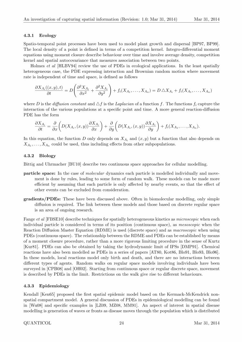
An investigation of capturing spatial information (Revision: 1.0; Mar 31, 2014) Mar 31, 2014

4.3.1 Ecology

Spatio-temporal point processes have been used to model plant growth and dispersal [BP97, BP99].The local density of a point is defined in terms of a competition kernel. Integro-differential momentequations using moment closure describe behaviour over time and involve average density, competitionkernel and spatial autocovariance that measures association between two points.

Holmes et al [HLBV94] review the use of PDEs in ecological applications. In the least spatiallyheterogeneous case, the PDE expressing interaction and Brownian random motion where movementrate is independent of time and space, is defined as follows

∂XAi((x, y), t)

∂t= D

(∂2XAi

∂x2+∂2XAi

∂y2

)+ fi(XA1 , . . . , XAn) = D4XAi + fi(XA1 , . . . , XAn)

where D is the diffusion constant and4f is the Laplacian of a function f . The functions fi capture theinteraction of the various populations at a specific point and time. A more general reaction-diffusionPDE has the form

∂XAi

∂t=

∂

∂x

(D(XAi , (x, y))

∂XAi

∂x

)+

∂

∂y

(D(XAi , (x, y))

∂XAi

∂y

)+ fi(XA1 , . . . , XAn).

In this equation, the function D only depends on XAi and (x, y) but a function that also depends onXA1 , . . . , XAn could be used, thus including effects from other subpopulations.

4.3.2 Biology

Bittig and Uhrmacher [BU10] describe two continuous space approaches for cellular modelling.

particle space: In the case of molecular dynamics each particle is modelled individually and move-ment is done by rules, leading to some form of random walk. These models can be made moreefficient by assuming that each particle is only affected by nearby events, so that the effect ofother events can be excluded from consideration.

gradients/PDEs: These have been discussed above. Often in biomolecular modelling, only simplediffusion is required. The link between these models and those based on discrete regular spaceis an area of ongoing research.

Fange et al [FBSE10] describe techniques for spatially heterogeneous kinetics as microscopic when eachindividual particle is considered in terms of its position (continuous space), as mesoscopic when theReaction Diffusion Master Equation (RDME) is used (discrete space) and as macroscopic when usingPDEs (continuous space). The relationship between the RDME and PDEs can be established by meansof a moment closure procedure, rather than a more rigorous limiting procedure in the sense of Kurtz[Kur81]. PDEs can also be obtained by taking the hydrodynamic limit of IPSs [DMP91]. Chemicalreactions have also been modelled as PDEs in a series of papers [AT80, Kot86, Blo91, Blo93, Blo96].In these models, local reactions model only birth and death, and there are no interactions betweendifferent types of agents. Random walks on regular space models involving individuals have beensurveyed in [CPB08] and [OH02]. Starting from continuous space or regular discrete space, movementis described by PDEs in the limit. Restrictions on the walk give rise to different behaviours.

4.3.3 Epidemiology

Kendall [Ken65] proposed the first spatial epidemic model based on the Kermack-McKendrick non-spatial compartment model. A general discussion of PDEs in epidemiological modelling can be foundin [Wu08] and specific examples in [LZ09, MZ08, MM91]. An aspect of interest in spatial diseasemodelling is generation of waves or fronts as disease moves through the population which is distributed

QUANTICOL 24 Mar 31, 2014

An investigation of capturing spatial information (Revision: 1.0; Mar 31, 2014) Mar 31, 2014

in space. Murray describes a two-dimensional continuous space model that takes into account localfox densities and carrying capacities of an outbreak of rabies in the south of England and extends it toconsider both natural immunity of foxes to rabies and size of breaks to curb the spread of the disease[Mur03]. A slightly different approach is taken in [BCG+09] where PDEs have diffusion terms thattake into account the concentration of the cholera in the water.

4.3.4 Networking

There is a substantial amount of work on mobility models, both at the analytical level and ex-perimentally through traces [CBD02]. Owing to its analytical tractability, the random walk (RW)model has been extensively studied in networking research. Unbiased RWs are proposed in [AHL96]and [ALLC00] to study movements across cellular networks, and to study routing protocols [IM06,GV06] and performance characteristics in ad hoc networks [GMPS04]. Direction based on an individ-ual’s state is a feature of a discrete time Markovian model developed for the comparison of updatestrategies in cellular networks [BNKS94]. RW is also used in [DT05] as the basic mobility modelto obtain a deterministic reaction-diffusion type equation for information propagation in ad hoc net-works, without considering it as a limit of a stochastic model. In [GL07], the PDEs interpreted as thedeterministic limit of node concentrations, by appealing to the strong law of large numbers.

4.4 Application to smart transport case studies

To date the examples considered within the QUANTICOL project, as described in the previous sec-tions, have focussed on discrete space except for the stochastic HYPE model of bike sharing (HYPE2bike) that uses continuous space, and a possible continuous space extension to the StocS bike sharingmodel (StocS bike extension). In the stochastic HYPE model of bike sharing (which is presented inDeliverable 4.1 [BFN+14]), space is a bounded continuous region. Users have an initial (x, y) locationand choose a random location to move to. If the distance to the location is sufficiently large, they willdecide to go by bike rather than walk. In each case, their speed and time taken is determined by theactual distance between points and their method of travel.

We can also consider the data we are working with. The location-at-time data we have obtainedfrom Lothian buses is spatially continuous, in that the data gathered from each bus at regular intervalscan be translated to 2-dimensional map coordinates (and then projected onto a 1-dimensional repre-sentation of route). Since this is not aggregated data, but data for individual buses, an appropriatespatial approach would be an agent-based system which simulates the movement of each bus.

The data is discrete time as it is not reported continuously and there are different approachesto developing a continuous time, discrete space model. In the first, the 2-dimensional data can beprojected onto a 1-dimensional route map, stops are identified and then fine division of the distancebetween stops is used to determine from the non-stop data how much time is spent in each division,and then a realistic model of bus movement can be derived [YGW+13]. This is a very fine-grainedapproach. In the second approach, which is coarser, the area of interest is divided into patches, andthe GPS data is analysed to determine rates of movements from one patch to another. This canbe done in a regular way, whether the area of interest is divided up into same sized patches, givinga regular discrete space model, or alternatively using geographical information, such as locations oftraffic lights or bus stops to give a irregular discrete space model. See Deliverable 5.1 [TCG+14] forfurther details.

5 Topological space models

Topological, distance, and closure spaces are suitable as the foundations of a simple, general mathemat-ical theory for representing and reasoning about various kinds of spatial models, Space is represented

QUANTICOL 25 Mar 31, 2014

An investigation of capturing spatial information (Revision: 1.0; Mar 31, 2014) Mar 31, 2014

as a set of points equipped with some additional structure. Functions that operate on space, or spa-tially distributed entities (for example, the dynamics of a system) are constrained to preserve thestructure. For a technical introduction to the subject, the report [CLM14] is available; furthermore,a brief account of spatial logics, can be found in Deliverable D3.1 [MBC+14].

Topological spaces. Topological spaces are best suited to represent continuous space. A topologicalspace is a set X equipped with a set of subsets of X, called open sets, which are closed under unionand finite intersection. Open sets play the role of constraints to functions, ensuring that continuityis well-defined. For example, a function representing movement of entities in continuous space mustbe “smooth” with respect to the open sets, ensuring that no discontinuous “jump” is possible. Anexample is the Euclidean plane R2 where the open sets are generated by union and finite intersectionof open balls, namely “circles without borders”.

Closure spaces. Closure spaces are better suited than topological spaces to model discrete spatialstructures. A closure space is a set X equipped with a closure operator subject to some axioms. Theidea of a closure operator is to add to a set the “least possible enlargement” of it. Closure operatorshave been studied and applied in the context of computer graphics and image processing. A closureoperator can be derived from the open sets of a topological space, making topological spaces a subclassof closure spaces. Closure spaces are also induced by regular grids, and more generally, by graphs.

Metric and distance spaces. Metric spaces have a binary, symmetric distance operator obeyingthe triangular inequality. Distance spaces relax any or all of these constraints. Distance spaces andtheir variants can be used to describe physical distances and they can be generalised so that costs canbe associated with pairs of points in the space. This aspect is orthogonal to the fact that a modelmay use continuous or discrete space. A classical example of a metric space is the Euclidean planeequipped with the Euclidean distance. When dealing with distances, one may sometimes resort topseudo-metrics where two different points may have null distance.

The abstract spaces that we introduced have in common a remarkable definitional simplicity. Never-theless, the basic axioms result in a rich theory, finding applications in several, apparently unrelateddomains.

5.1 Examples of existing use

Topological and metric spaces are widely known and used throughout mathematics, physics, engi-neering, and computer science. As is typical with abstractions, it is not obvious to point at specificapplications, since the abstractions are mostly used to ease the development of general mathematicaltheories which are then instantiated to concrete examples. Relating to the QUANTICOL project,topology and distance are used to provide models of spatial logics. Spatial logics are used to describeproperties of space [APHvB07] and selected topics have been summarised in the technical report[CLM14], and in Deliverable D3.1 [MBC+14]. The advantage of using abstract spaces as models ofa logic is the ability to give a uniform definition of logical operators, that encompasses a wide rangeof cases; for example, one may define a logic that describes equally well objects moving in planes,three-dimensional spaces, space-time, discrete regular grids and arbitrary graphs. Moreover, one isable to separate concerns with respect to the features of a logical language. In particular, the notionof distance is orthogonal to that of continuous movement and therefore, one may adopt models thatcan be viewed both as metric and as topological spaces. By adhering to the existing mathematicaltradition, we expect to be able to reuse such knowledge, in order to provide a general verificationframework for the QUANTICOL case studies, without reinventing theory.

QUANTICOL 26 Mar 31, 2014

An investigation of capturing spatial information (Revision: 1.0; Mar 31, 2014) Mar 31, 2014

5.2 Application to smart transport case studies

In the smart transport case studies it is fundamental to take into account a map providing informationon how movement of entities in space is constrained. A map may be described topologically andmetrically. Topologically, the various interesting regions of a map (streets, parking lots, rivers, etc.)may be described as predicates over the points of a topological space (or a closure space, in the discretecase). Principles of continuity of change (that exist even in the discrete case) permit one to deriveinteresting conclusions about given configurations of a model, for example, reachability of a parkinglot from relevant points of interest. Typically, we expect that models in the smart transport casestudies are discrete. In some cases, when considering the graph obtained from a map or topologicalmap of bus and bike stations of a town, space is discrete. In some other cases, discreteness merelycomes as an approximation of continuity. As a simple example, consider smart-lock applications inbike sharing. By using a digitally enhanced lock, customers may leave a bike at arbitrary (continuous)coordinates on the map.

Furthermore, continuity may allow reasoning about spatial abstraction in the sense that a complexmap may be continuously transformed to a less complex one that still provides important informationabout the ability to find a path from one point to another. This may allow for the construction of atopological map from a map, as described in Section 2.

Distances may be added on top of this basic framework, with different meanings. One may considerjust physical distance between points. More generally, a distance may represent a cost. For example,in the bike sharing scenario, it is relevant to know whether a point of interest is on top of a hill;the cost of moving a bike may be different for different stations, even though the physical distanceis the same. In a bus network, urban and extra-urban rides may have different costs. Anotherexample of a distance is the time needed to move between points, which may be only loosely related tophysical distance (consider for example, road traffic and peak hours). Costs may be combined whenconsidering integrated bus and bike sharing scenarios, giving rise to complex use cases that requiresome abstraction to be treated satisfactorily. We expect that abstract modelling of space will allowus to extrapolate the interesting common features among the variety of cases that we depicted, andto be able to derive a reasoning and automated verification framework that is suitable to derive usefulpredictions in the smart transport case studies.

6 Conclusion

6.1 The classification revisited

We can now apply the classification to the QUANTICOL case studies and this is shown in Figure 6.As can be seen, there is a fair distribution across the table. As mentioned previously, the techniquesthat fall into column two differ from the usual approaches that have been taken in prior research bythe members of this project, as it involves considering individuals and continuous quantities. We nowconsider what could fill the empty positions in the table.

Discrete homogeneous space, no aggregation: An extension of the CTMC route model couldsee quantities such as power consumption associated with individual buses which would fit intothis category. If individual buses also have a discrete state (for example, whether they are ontime or not), then this could result in a continuous time, homogeneous space model withoutstate aggregation where there are both discrete state and continuous state variables. This wouldbe a hybrid model.

Discrete space, continuous state, no aggregation: Similarly to the case above, one could extendany of the models under discrete state to include some continuous value, and this extension wouldbe a hybrid model.

QUANTICOL 27 Mar 31, 2014

An investigation of capturing spatial information (Revision: 1.0; Mar 31, 2014) Mar 31, 2014

Time continuous or discreteAggr none state and/or spaceState discrete continuous discrete continuous

Spacediscrete

general PEPA bus PEPA busHYPE bus PALOMA bike

HYPE1 bike EPFL2 bikeStoKlaim bike StocS bike

PEPA-S bikeBio-PEPA bike

CTMC bike

regular CTMC route EPFL1 bike

homo- EPFL1 bikegeneous DTMC bike

continuous HYPE2 bikeStocS bikeextension

Figure 6: Classification of QUANTICOL case studies in terms of time, aggregation, state and space

Continuous space, no aggregation: Only one slot is filled; however, as the project progresses, wemay find that there are some models without aggregation for which continuous space is importantfor reasons of accuracy.

Continuous space, continuous-state aggregation: It is unclear whether PDEs will play a rolein this project, as it seems unlikely that the kind of diffusion and dispersal represented by thistechnique has a role in modelling smart transport, unless we model passenger movement bothon and off buses.

Looking at Figure 6, the focus has been on individual models with discrete space (with continuous ordiscrete time), and population models with discrete space, both discrete and continuous populations.This suggests that these techniques are the appropriate techniques for modelling smart transport, andthat we should not be trying to construct models in other categories just because space modellingtechniques exist for these categories. However, our choice of modelling techniques must also be deter-mined by our modelling goals and the questions we wish to answer through modelling. At this stageof the project, we have a partial list of these goals or these questions. Hence, choice of modellingtechnique (within reasonable bounds) may evolve as the project proceeds.

6.2 Conclusions

The following points summarise the main conclusions about the mathematical techniques for spatialmodelling that have been obtained from the literature and relating to the QUANTICOL case studies.

• The techniques in the literature seem to use well-understood theory of difference and differentialequations, in particular, those differential equations that are easy to solve numerically. For thesmart transport case studies in QUANTICOL, we may need to use more complex ODEs.

QUANTICOL 28 Mar 31, 2014

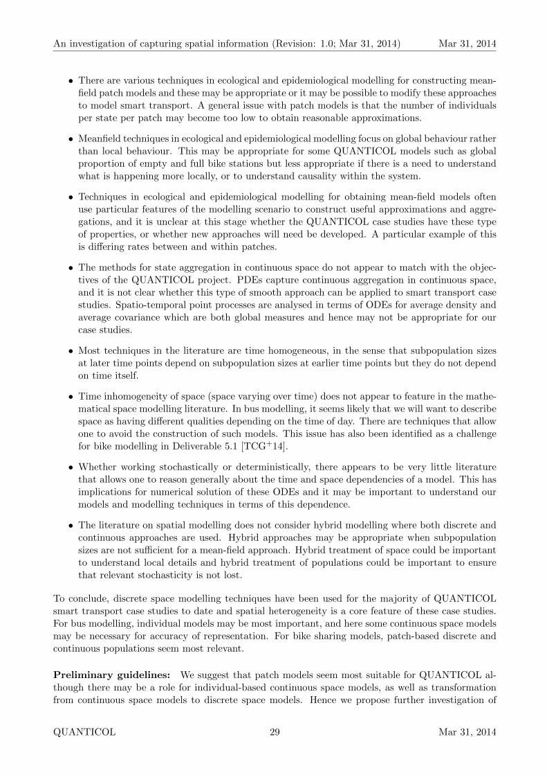
An investigation of capturing spatial information (Revision: 1.0; Mar 31, 2014) Mar 31, 2014

• There are various techniques in ecological and epidemiological modelling for constructing mean-field patch models and these may be appropriate or it may be possible to modify these approachesto model smart transport. A general issue with patch models is that the number of individualsper state per patch may become too low to obtain reasonable approximations.

• Meanfield techniques in ecological and epidemiological modelling focus on global behaviour ratherthan local behaviour. This may be appropriate for some QUANTICOL models such as globalproportion of empty and full bike stations but less appropriate if there is a need to understandwhat is happening more locally, or to understand causality within the system.

• Techniques in ecological and epidemiological modelling for obtaining mean-field models oftenuse particular features of the modelling scenario to construct useful approximations and aggre-gations, and it is unclear at this stage whether the QUANTICOL case studies have these typeof properties, or whether new approaches will need be developed. A particular example of thisis differing rates between and within patches.

• The methods for state aggregation in continuous space do not appear to match with the objec-tives of the QUANTICOL project. PDEs capture continuous aggregation in continuous space,and it is not clear whether this type of smooth approach can be applied to smart transport casestudies. Spatio-temporal point processes are analysed in terms of ODEs for average density andaverage covariance which are both global measures and hence may not be appropriate for ourcase studies.

• Most techniques in the literature are time homogeneous, in the sense that subpopulation sizesat later time points depend on subpopulation sizes at earlier time points but they do not dependon time itself.

• Time inhomogeneity of space (space varying over time) does not appear to feature in the mathe-matical space modelling literature. In bus modelling, it seems likely that we will want to describespace as having different qualities depending on the time of day. There are techniques that allowone to avoid the construction of such models. This issue has also been identified as a challengefor bike modelling in Deliverable 5.1 [TCG+14].

• Whether working stochastically or deterministically, there appears to be very little literaturethat allows one to reason generally about the time and space dependencies of a model. This hasimplications for numerical solution of these ODEs and it may be important to understand ourmodels and modelling techniques in terms of this dependence.

• The literature on spatial modelling does not consider hybrid modelling where both discrete andcontinuous approaches are used. Hybrid approaches may be appropriate when subpopulationsizes are not sufficient for a mean-field approach. Hybrid treatment of space could be importantto understand local details and hybrid treatment of populations could be important to ensurethat relevant stochasticity is not lost.

To conclude, discrete space modelling techniques have been used for the majority of QUANTICOLsmart transport case studies to date and spatial heterogeneity is a core feature of these case studies.For bus modelling, individual models may be most important, and here some continuous space modelsmay be necessary for accuracy of representation. For bike sharing models, patch-based discrete andcontinuous populations seem most relevant.

Preliminary guidelines: We suggest that patch models seem most suitable for QUANTICOL al-though there may be a role for individual-based continuous space models, as well as transformationfrom continuous space models to discrete space models. Hence we propose further investigation of

QUANTICOL 29 Mar 31, 2014

An investigation of capturing spatial information (Revision: 1.0; Mar 31, 2014) Mar 31, 2014

mean-field models to understand which techniques are useful and also to possibly develop new ap-proaches, consideration of spatial moment closure techniques for both global and local measures, andexploration of hybrid approaches for space modelling.

Relationships with other deliverables and work packages:

WP1 Emergent Behaviour and Adaptivity: The work in Work Package 1 on multiscale modelling[BGH+14] may be relevant for spatial modelling as we may wish to model at different spatialscales and the work on temporal scales may also be applicable. This may be particularly impor-tant when rates within patches operate on a different timescale to those between patches. Task1.3 looks at language and analysis techniques and space has a role to play in this task as well.Furthermore, mean-field techniques are important when working with patch models.

WP3 Logic and Scalable Verification: Work Package 3 includes spatial logics for model checking tech-niques that will exploit mean-field approximation, and hence Deliverable 2.1 is relevant becauseit contributes to finding suitable spatial representations.

WP4 Language and Design Methodology: Deliverable 2.1 may indirectly influence Work Package 4as it will be used to determine process algebraic features that will be described in the internalreport of Task 2.2 that will then become part of the CAS-SCEL language.

WP5 Model Validation and Tool Support: Deliverable 2.1 influences WP5 as it provides guidelinesfor spatial modelling, and it is also influenced by the requirements identified for the case studiesin the project [TCG+14].

Work plan for the second reporting period: The DOW describes three tasks in Work Package 2.

T2.1 Scalable representations of space (started, ends month 42)

T2.2 Stochastic process algebras for spatial aspects (starts month 25, ends month 48)

T2.3 Parameter and model fitting from spatial data (starts month 19, ends month 36)

The second phase of Task 2.1 will now begin and this involves preparing the internal report titled“A unified view of spatial representation and analysis techniques”. In this phase, the ways in whichthe different spatial modelling techniques can be analysed will be investigated further, providing anunderstanding of the costs of various methods, and allowing for appropriate choices for modelling theQUANTICOL case studies. Additionally the items proposed above will be investigated.

Task 2.3 starts in October 2014 and will consider parameterisation of space for spatial models.Deliverable 2.1 and its associated technical report will provide a starting point for this research, as anumber of papers referenced consider parameterisation. Deliverable 2.2 will document this task andis due in month 36 (end of March 2016) at the end of the task.

Looking further forward, Task 2.2 will start in April 2015, and its internal report is due in month30 (end of September 2015). This report will be an investigation of space modelling in stochasticprocess algebras.

Acknowledgements

We thank members of the advisory board of the QUANTICOL project for their helpful comments.

QUANTICOL 30 Mar 31, 2014

An investigation of capturing spatial information (Revision: 1.0; Mar 31, 2014) Mar 31, 2014

References

[ADH+05] J. Arino, J.R. Davis, D. Hartley, R. Jordan, J.M. Miller, and P. van den Driessche. A multi-speciesepidemic model with spatial dynamics. Mathematical Medicine and Biology, 22(2):129–142, 2005.

[AHL96] I.F. Akyildiz, J.S.M. Ho, and Y.-B. Lin. Movement-based location update and selective paging forPCS networks. IEEE/ACM Transactions on Networking, 4(4):629–638, 1996.

[ALLC00] I.F. Akyildiz, Y.-B. Lin, W.-R. Lai, and R.-J. Chen. A new random walk model for PCS networks.IEEE Journal on Selected Areas in Communications, 18(7):1254–1260, 2000.

[AMR95] U.M. Ascher, R.M.M. Mattheij, and R.D. Russell. Numerical solution of boundary value problemsfor ordinary differential equations. SIAM, 1995.

[AP02] F. Arrigoni and A. Pugliese. Limits of a multi-patch SIS epidemic model. Journal of MathematicalBiology, 45(5):419–440, November 2002.

[APHvB07] M. Aiello, I. Pratt-Hartmann, and J. van Benthem, editors. Handbook of Spatial Logics. Springer,2007.

[APS12] P. Auger, J.C. Poggiale, and E. Sanchez. A review on spatial aggregation methods involving severaltime scales. Ecological Complexity, 10:12–25, June 2012.

[AT80] L. Arnold and M. Theodosopulu. Deterministic limit of the stochastic model of chemical reactionswith diffusion. Advances in Applied Probability, 12(2):367–379, 1980.

[AvdD03] J. Arino and P. van den Driessche. A multi-city epidemic model. Mathematical Population Studies,10(3):175–193, 2003.

[BBS07] A. Baddeley, I. Barany, and R. Schneider. Spatial point processes and their applications. StochasticGeometry: Lectures given at the CIME Summer School 2004, page 175, 2007.

[BCG+09] E. Bertuzzo, R. Casagrandi, M. Gatto, I. Rodriguez-Iturbe, and A. Rinaldo. On spatially explicitmodels of cholera epidemics. Journal of The Royal Society Interface, 7(43):321–333, 2009.

[Ber02] L. Berec. Techniques of spatially explicit individual-based models: construction, simulation, andmean-field analysis. Ecological Modelling, 150(1):5581, 2002.

[BFN+14] L. Bortolussi, C. Feng, R. De Nicola, J. Hillston, V. Galpin, D. Latella, M. Loreti, M. Massink,and V. Senni. CAS-SCEL language design. QUANTICOL Deliverable 4.1, March 2014.

[BG95] B. Bolker and B. Grenfell. Space, persistence and dynamics of measles epidemics. PhilosophicalTransactions of the Royal Society of London. Series B: Biological Sciences, 348(1325):309–320,1995.

[BGH+14] L. Bortolussi, N. Gast, J. Hillston, R. Paskauskas, and M. Tribastone. Multiscale modellinginformed by smart grids. QUANTICOL Deliverable 1.1, March 2014.

[BHLM13] L. Bortolussi, J. Hillston, D. Latella, and M. Massink. Continuous approximation of collectivesystems behaviour: a tutorial. Performance Evaluation, 70(5):317–349, 2013.

[BKHW05] C. Baier, J.-P. Katoen, H. Hermanns, and V. Wolf. Comparative branching-time semantics formarkov chains. Information and Computation, 200(2):149–214, 2005.

[BLM13] L. Bortolussi, D. Latella, and M. Massink. Stochastic process algebra and stability analysis ofcollective systems. In R. De Nicola and C. Julien, editors, 15th International Conference onCoordination Models and Languages (COORDINATION 2013), LNCS 7890, pages 1–15. Springer,2013.

[Blo91] D. Blount. Comparison of stochastic and deterministic models of a linear chemical reaction withdiffusion. The Annals of Probability, 19(4):1440–1462, 1991.

[Blo93] D. Blount. Limit theorems for a sequence of nonlinear reaction-diffusion systems. StochasticProcesses and their Applications, 45(2):193–207, 1993.

[Blo96] D. Blount. Diffusion limits for a nonlinear density dependent space-time population model. TheAnnals of Probability, 24(2):639–659, 1996.

QUANTICOL 31 Mar 31, 2014

An investigation of capturing spatial information (Revision: 1.0; Mar 31, 2014) Mar 31, 2014

[BNKS94] A. Bar-Noy, I. Kessler, and M. Sidi. Mobile users: To update or not to update? In INFOCOM1994, pages 570–576, 1994.

[BP97] B. Bolker and S.W. Pacala. Using moment equations to understand stochastically driven spatialpattern formation in ecological systems. Theoretical population biology, 52(3):179–197, 1997.

[BP99] B.M. Bolker and S.W. Pacala. Spatial moment equations for plant competition: Understandingspatial strategies and the advantages of short dispersal. The American Naturalist, 153(6):575–602,1999.

[BP10] L. Bortolussi and A. Policriti. Hybrid dynamics of stochastic programs. Theoretical ComputerScience, 411:2052–2077, 2010.

[Bra08] F. Brauer. Compartmental models in epidemiology. In L.J.S. Allen, F. Brauer, P. van den Driessche,and J. Wu, editors, Mathematical Epidemiology, pages 19–80. Springer, 2008.

[Bru67] S.G. Brush. History of the Lenz-Ising model. Reviews of Modern Physics, 39(4):883, 1967.

[BU10] A.T. Bittig and A.M. Uhrmacher. Spatial modeling in cell biology at multiple levels. In WinterSimulation Conference (WSC 2010), pages 608–619. IEEE, 2010.

[CBD02] T. Camp, J. Boleng, and V. Davies. A survey of mobility models for ad hoc network research.Wireless Communications and Mobile Computing, 2(5):483–502, 2002.

[CFB09] H. Conceicao, M. Ferreira, and J. Barros. A cautionary view of mobility and connectivity modelingin vehicular ad-hoc networks. In IEEE 69th Vehicular Technology Conference (VTC 2009), pages1–5. IEEE, 2009.

[CGB+10] D. Cerotti, M. Gribaudo, A. Bobbio, C.T. Calafate, and P. Manzoni. A Markovian agent modelfor fire propagation in outdoor environments. In Seventh European Performance EngineeringWorkshop (EPEW 2010), LNCS 6342, pages 131–146. Springer, 2010.

[Che81] P.L. Chesson. Models for spatially distributed populations: the effect of within-patch variability.Theoretical Population Biology, 19(3):288–325, 1981.

[Che12] P. Chesson. Scale transition theory: its aims, motivations and predictions. Ecological Complexity,10:52–68, 2012.

[CHK+05] R. Chaturvedi, C. Huang, B. Kazmierczak, T. Schneider, J.A. Izaguirre, T. Glimm, H.G.E.Hentschel, J.A. Glazier, S.A. Newman, and M.S. Alber. On multiscale approaches to three-dimensional modelling of morphogenesis. Journal of the Royal Society Interface, 2(3):237–253,2005.

[CL07] P.M. Chaikin and T.C. Lubensky. Principles of Condensed Matter Physics. Cambridge UniversityPress, 4th edition, 2007.

[CLBR09] A. Chaintreau, J.-Y. Le Boudec, and N. Ristanovic. The age of gossip: spatial mean field regime.In Eleventh International Joint Conference on Measurement and Modeling of Computer Systems(SIGMETRICS/Performance 2009), pages 109–120. ACM, 2009.

[CLM14] V. Ciancia, D. Latella, and M. Massink. Logics of space and time. Technical Report TR-QC-01-2014, QUANTICOL, 2014.

[CMRM07] R. Calegari, M. Musolesi, F. Raimondi, and C. Mascolo. CTG: a connectivity trace generatorfor testing the performance of opportunistic mobile systems. In 6th Joint Meeting of the Euro-pean Software Engineering Conference and the ACM SIGSOFT Symposium on the Foundations ofSoftware Engineering, pages 415–424. ACM, 2007.

[CPB08] E.A Codling, M.J Plank, and S. Benhamou. Random walk models in biology. Journal of the RoyalSociety Interface, 5(25):813–834, 2008.

[Dav93] M.H.A. Davis. Markov Models and Optimization. Chapman & Hall, 1993.

[DL94a] R. Durrett and S. Levin. The importance of being discrete (and spatial). Theoretical PopulationBiology, 46(3):363–394, 1994.

[DL94b] R. Durrett and S.A. Levin. Stochastic spatial models: a user’s guide to ecological applications.Philosophical Transactions of the Royal Society B: Biological Sciences, 343(1305):329–350, 1994.

QUANTICOL 32 Mar 31, 2014

An investigation of capturing spatial information (Revision: 1.0; Mar 31, 2014) Mar 31, 2014

[DMP91] A. De Masi and E. Presutti. Mathematical methods for hydrodynamic limits. Lecture Notes inMathematics. Springer-Verlag, 1991.

[DN08] R.W.R. Darling and J.R. Norris. Differential equation approximations for Markov chains. Proba-bility surveys, 5:37–79, 2008.

[DP03] J. Desharnais and P. Panangaden. Continuous stochastic logic characterizes bisimulation ofcontinuous-time markov processes. The Journal of Logic and Algebraic Programming, 56(1-2):99–115, 2003.

[DT05] M. Durvy and P. Thiran. Reaction-diffusion based transmission patterns for ad hoc networks. InINFOCOM 2005, volume 3, pages 2195–2205, 2005.

[EE04] J. Elf and M. Ehrenberg. Spontaneous separation of bi-stable biochemical systems into spatialdomains of opposite phases. Systems Biology, 1(2):230–236, 2004.

[FBSE10] D. Fange, O.G. Berg, P. Sjoberg, and J. Elf. Stochastic reaction-diffusion kinetics in the microscopiclimit. Proceedings of the National Academy of Sciences, 107(46):19820–19825, 2010.

[Fen14] C. Feng. Patch-based hybrid modelling of spatially distributed systems by using stochastic HYPE– ZebraNet as an example. In Twelve International Workshop on Quantitative Aspects of Pro-gramming Languages and Systems (QAPL 2014), 2014.

[FG12] C. Fricker and N. Gast. Incentives and regulations in bike-sharing systems with stations of finitecapacity. arXiv preprint arXiv:1201.1178, 2012.

[FGM12] C. Fricker, N. Gast, and H. Mohamed. Mean field analysis for inhomogeneous bike sharing systems.DMTCS Proceedings, 01:365–376, 2012.

[FS86] O. Frank and D. Strauss. Markov graphs. Journal of the American Statistical Association,81(395):832–842, 1986.

[Gar76] A. Gardiner. Homogeneous graphs. Journal of Combinatorial Theory, Series B, 20(1):94–102,1976.

[GFH+14] V. Galpin, C. Feng, J. Hillston, M. Massink, M. Tribastone, and M. Tschaikowski. Review of time-based techniques for modelling space. Technical Report TR-QC-05-2014, QUANTICOL, 2014.

[GG92] F. Graner and J.A. Glazier. Simulation of biological cell sorting using a two-dimensional extendedpotts model. Physical Review Letters, 69(13):2013, 1992.

[Gil97] D.T. Gillespie. Exact stochastic simulation of coupled chemical reactions. Journal of PhysicalChemistry, 81(25):2340–2361, 1997.

[GL07] M. Garetto and E. Leonardi. Analysis of random mobility models with partial differential equations.IEEE Transactions on Mobile Computing, 6(11):1204–1217, 2007.

[GMB+12] M. Gatto, L. Mari, E. Bertuzzo, R. Casagrandi, L. Righetto, I. Rodriguez-Iturbe, and A. Ri-naldo. Generalized reproduction numbers and the prediction of patterns in waterborne disease.Proceedings of the National Academy of Sciences, 109(48):19703–19708, 2012.

[GMPS04] A.El. Gamal, J. Mammen, B. Prabhakar, and D. Shah. Throughput-delay trade-off in wirelessnetworks. In INFOCOM 2004, 2004.

[GMWM76] C.W. Gardiner, K.J. McNeil, D.F. Walls, and I.S. Matheson. Correlations in stochastic theoriesof chemical reactions. Journal of Statistical Physics, 14(4):307–331, 1976.

[Gre92] B.T. Grenfell. Chance and chaos in measles dynamics. Journal of the Royal Statistical Society.Series B (Methodological), 54(2):383–398, 1992.

[GV06] M. Grossglauser and M. Vetterli. Locating mobile nodes with EASE: learning efficient routes fromencounter histories alone. IEEE/ACM Transactions on Networks, 14(3):457–469, 2006.

[HCM91] M.P. Hassell, H.N. Comins, and R.M. May. Spatial structure and chaos in insect populationdynamics. Nature, 353(6341):255–258, 1991.

[HLBV94] E.E. Holmes, M.A. Lewis, J.E. Banks, and R.R. Veit. Partial differential equations in ecology:spatial interactions and population dynamics. Ecology, 75(1):17–29, 1994.

QUANTICOL 33 Mar 31, 2014

An investigation of capturing spatial information (Revision: 1.0; Mar 31, 2014) Mar 31, 2014

[Ila01] A. Ilachinski. Cellular automata: a discrete universe. World Scientific, 2001.

[IM06] S. Ioannidis and P. Marbach. A Brownian motion model for last encounter routing. In INFOCOM2006, 2006.

[Isa08] S.A. Isaacson. Relationship between the reaction–diffusion master equation and particle trackingmodels. Journal of Physics A: Mathematical and Theoretical, 41(6):065003, 2008.

[Kan98] K. Kaneko. Diversity, stability, and metadynamics: Remarks from coupled map studies. InJ. Bascompte and R.V. Sole, editors, Modeling spatiotemporal dynamics in ecology, pages 27–45.Springer-Verlag, 1998.

[Ken65] D.G. Kendall. Mathematical models of the spread of infection. In Mathematics and ComputerScience in Biology and Medicine, pages 213–225. Medical Research Council London, 1965.

[Kot86] P. Kotelenez. Law of large numbers and central limit theorem for linear chemical reactions withdiffusion. The Annals of Probability, 14(1):173–193, 1986.

[KP07] T. Kathiravelu and A. Pears. Reproducing opportunistic connectivity traces using connectivitymodels. In 2007 ACM CoNEXT conference, page 34. ACM, 2007.

[KS76] J.G. Kemeny and J.L. Snell. Finite Markov chains: with a new appendix: Generalization of afundamental matrix. Springer, New York, 1976.

[Kur81] T.G. Kurtz. Approximation of population processes. SIAM, 1981.

[LD96] S.A. Levin and R. Durrett. From individuals to epidemics. Philosophical Transactions of the RoyalSociety of London. Series B: Biological Sciences, 351(1347):1615–1621, 1996.

[Lev69] R. Levins. Some demographic and genetic consequences of environmental heterogeneity for bio-logical control. Bulletin of the ESA, 15(3):237–240, 1969.

[Lev74] S.A. Levin. Dispersion and population interactions. American Naturalist, 108(960):207–228, 1974.

[LLM13] D. Latella, M. Loreti, and M. Massink. On-the-fly PCTL fast mean-field model-checking for self-organising coordination – preliminary version. Technical Report TR-QC-01-2013, QUANTICOL,2013.

[LZ09] J. Li and X. Zou. Modeling spatial spread of infectious diseases with a fixed latent period in aspatially continuous domain. Bulletin of mathematical biology, 71(8):20482079, 2009.

[MBC+14] M. Massink, L. Bortolussi, V. Ciancia, J. Hillston, A. Lluch-Lafuente, D. Latella, M. Loreti, D. Rei-jsbergen, and A. Vandin. Foundations of scalable verification for stochastic logics. QUANTICOLDeliverable 3.1, March 2014.

[MBL+13] M. Massink, M. Brambilla, D. Latella, M. Dorigo, and M. Birattari. On the use of Bio-PEPAfor modelling and analysing collective behaviors in swarm intelligence. Swarm Intelligence, 7(2-3):201–228, 2013.

[MBR+12] L. Mari, E. Bertuzzo, L. Righetto, R. Casagrandi, M. Gatto, I. Rodriguez-Iturbe, and A. Rinaldo.Modelling cholera epidemics: the role of waterways, human mobility and sanitation. Journal ofThe Royal Society Interface, 9(67):376–388, 2012.

[MLB+12] M. Massink, D. Latella, A. Bracciali, M.D. Harrison, and J. Hillston. Scalable context-dependentanalysis of emergency egress models. Formal Aspects of Computing, 24(2):267–302, 2012.

[MM91] D.B. Meade and F.A. Milner. An SIR model for epidemics with diffusion to avoid infectionand overcrowding. In 13th IMACS World Congress on Computation and Applied Mathematics,volume 3, pages 1444–1445, 1991.

[MMRL02] G. Marion, X. Mao, E. Renshaw, and J. Liu. Spatial heterogeneity and the stability of reactionstates in autocatalysis. Physical Review E, 66(5):051915, November 2002.

[MNS11] C. McCaig, R. Norman, and C. Shankland. From individuals to populations: a mean field semanticsfor process algebra. Theoretical Computer Science, 412(17):1557–1580, 2011.

[Mol77] D. Mollison. Spatial contact models for ecological and epidemic spread. Journal of the RoyalStatistical Society. Series B (Methodological), 39(3):283–326, 1977.

QUANTICOL 34 Mar 31, 2014

An investigation of capturing spatial information (Revision: 1.0; Mar 31, 2014) Mar 31, 2014

[MP12] A. Morozov and J.-C. Poggiale. From spatially explicit ecological models to mean-field dynamics:the state of the art and perspectives. Ecological Complexity, 10:1–11, 2012.

[MSH05] G. Marion, D.L. Swain, and M.R. Hutchings. Understanding foraging behaviour in spatially het-erogeneous environments. Journal of Theoretical Biology, 232(1):127–142, 2005.

[Mur02] J.D. Murray. Mathematical Biology I: An Introduction. Springer, 3rd edition, 2002.

[Mur03] J.D. Murray. Mathematical biology II: Spatial Models and Biomedical Applications. Springer, NewYork, 2003.

[MVZ05] M. Mamei, M. Vasirani, and F. Zambonelli. Self-organizing spatial shapes in mobile particles: theTOTA approach. In Engineering Self-Organising Systems, pages 138–153. Springer, 2005.

[MZ08] F.A. Milner and R. Zhao. SIR model with directed spatial diffusion. Mathematical PopulationStudies, 15(3):160–181, 2008.

[Nor98] J.R. Norris. Markov chains. Cambridge University Press, 1998.

[OH02] H.G. Othmer and T. Hillen. The diffusion limit of transport equations II: chemotaxis equations.SIAM Journal on Applied Mathematics, 62(4):1222–1250, 2002.

[OL01] A. Okubo and S. A. Levin. Diffusion and ecological problems: modern perspectives. Springer, 2001.

[OS71] H.G. Othmer and L.E. Scriven. Instability and dynamic pattern in cellular networks. Journal oftheoretical biology, 32(3):507–537, 1971.

[Pan09] P. Panangaden. Labelled Markov Processes. Imperial College Press, 2009.

[PRL11] M. Pascual, M. Roy, and K. Laneri. Simple models for complex systems: exploiting the relationshipbetween local and global densities. Theoretical Ecology, 4(2):211–222, 2011.

[RA97] C.J. Rhodes and R.M. Anderson. Epidemic thresholds and vaccination in a lattice model of diseasespread. Theoretical Population Biology, 52(2):101–118, 1997.

[RG03] J. E. Rowe and R. Gomez. El Botellon: Modeling the movement of crowds in a city. ComplexSystems, 14:363–370, 2003.

[Ril07] S. Riley. Large-scale spatial-transmission models of infectious disease. Science, 316(5829):1298–1301, 2007.

[SBG02] F.P. Schoenberg, D.R. Brillinger, and P. Guttorp. Point processes, spatial–temporal. In Encyclo-pedia of environmetrics, volume 3, pages 1573–1577. Wiley Online Library, 2002.

[SSML03] B.M. Slepchenko, J.C. Schaff, I. Macara, and L.M. Loew. Quantitative cell biology with the virtualcell. Trends in cell biology, 13(11):570–576, 2003.

[Tak96] Y. Takeuchi. Global dynamical properties of Lotka-Volterra systems. World Scientific, 1996.

[TCG+14] M. Tribastone, A. Clark, N. Gast, S. Gilmore, and D. Reijsbergen. Data validation and require-ments for case studies. QUANTICOL Deliverable 5.1, March 2014.

[TGH12] M. Tribastone, S. Gilmore, and J. Hillston. Scalable Differential Analysis of Process AlgebraModels. IEEE Transactions on Software Engineering, 38(1):205–219, 2012.

[TT13] M. Tschaikowski and M. Tribastone. Spatial fluid limits for stochastic mobile networks. arXivpreprint arXiv:1307.4566, 2013.

[Tur53] A.M. Turing. The chemical basis of morphogenesis. Philosophical Transactions of the Royal Society(Part B), 237:37–72, 1953.

[Van07] N. G. Van Kampen. Stochastic Processes in Physics and Chemistry. Elsevier, 3rd edition, 2007.

[VBU13] M. Viroli, J. Beal, and K. Usbeck. Operational semantics of proto. Science of Computer Program-ming, 78(6):633–656, 2013.

[vdD08] P. van den Driessche. Spatial structure: Patch models. In L.J.S. Allen, F. Brauer, P. van denDriessche, and J. Wu, editors, Mathematical Epidemiology, pages 179–190. Springer, 2008.

[Wik13a] Wikipedia. Lattice graph, 2013. Last accessed: 4 Feb 2013, http://en.wikipedia.org/wiki/Lattice_graph.

QUANTICOL 35 Mar 31, 2014

An investigation of capturing spatial information (Revision: 1.0; Mar 31, 2014) Mar 31, 2014

[Wik13b] Wikipedia. Topological map, 2013. Last accessed: 4 Feb 2013, http://en.wikipedia.org/wiki/Topological_map.

[WKB07] S.D. Webb, M.J. Keeling, and M. Boots. Host-parasite interactions between the local and themean-field: how and when does spatial population structure matter? Journal of TheoreticalBiology, 249(1):140–152, 2007.

[WL95] J. Wu and O.L. Loucks. From balance of nature to hierarchical patch dynamics: a paradigm shiftin ecology. The Quarterly Review of Biology, 70(4):439–466, 1995.

[Wu08] J. Wu. Spatial structure: partial differential equations models. In L.J.S. Allen, F. Brauer,P. van den Driessche, and J. Wu, editors, Mathematical Epidemiology, pages 191–204. Springer,2008.

[XFAS06] D. Xu, Z. Feng, L.J.S. Allen, and R.K. Swihart. A spatially structured metapopulation modelwith patch dynamics. Journal of Theoretical Biology, 239(4):469–481, 2006.

[YGW+13] Y. Yang, D. Gerstle, P. Widhalm, D. Bauer, and M.C. Gonzalez. The potential of low-frequencyAVL data for the monitoring and control of bus performance. In Transportation Research Board92nd Annual Meeting, pages 13–4011, 2013.

Appendix: Discrete and continuous time Markov chains

This section briefly introduces these concepts, as they would be used in stochastic modelling both with-out aggregation of state and with aggregation of state (population-based Markov chains) [BKHW05,BHLM13].

Definition 1. A discrete time Markov chain (DTMC) is a tuple MD = (S,P) where

• S is a finite set of states, and

• P : S × S → [0, 1] is a probability matrix satisfying∑

S′∈S P(S, S′) = 1 for all S ∈ S.

A DTMC is time-abstract [BKHW05] in the sense that time is viewed as a sequence of discrete stepsor clock ticks. It describes behaviour as follows: if an entity or individual is currently in state S ∈ Sthen the probability of the entity being in state S′ at the next time step is defined by P(S, S′). Undercertain conditions, the steady state of the DTMC can be determined and this describes when theDTMC is at equilibrium and gives the (unchanging) probability of being in any of the states of S. Bycontrast, transient state probabilities can be determined at each point in time before steady state isachieved.

Definition 2. A continuous time Markov chain (CTMC) is a tuple MC = (S,R) where

• S is a finite set of states, and

• R : S × S → R≥0 is a rate matrix.

CTMCs are time-aware [BKHW05] since they use continuous time. If an entity is currently in stateS, then R(S, S′) is a non-negative number that defines an exponential distribution from which theduration of the time taken to transition from state S to state S′ can be drawn. As with DTMCs andunder certain conditions, transient and steady state probabilities can be calculated which describe theprobability of being in each state at a particular time t or in the long run, respectively.

Let E(S) =∑

S′∈S R(S, S′) be the exit rate of state S′. Then the embedded DTMC of a CTMChas entries in its probability matrix of the form P(S, S′) = R(S, S′)/E(S) if E(S) > 0 and P(S, S′) = 0otherwise. DTMCs and CTMCs can be state-labelled (usually with propositions) or transition-labelled(usually with actions). The research in QUANTICOL focusses on transition-labelled Markov chains.We next consider population Markov chains, both discrete time and continuous time. Instead ofconsidering an entity with states, we now consider a vector of counts X that describes how manyentities are in each state; thus it is a population view rather than an individual view.

QUANTICOL 36 Mar 31, 2014

An investigation of capturing spatial information (Revision: 1.0; Mar 31, 2014) Mar 31, 2014

Definition 3. A population discrete time Markov chain (PDTMC) is a tuple XD = (X,D, T ) where

• X = (X1, . . . , Xn) is a vector of variables

• D is a countable set of states defined as D = D1 × . . . × Dn where each Di ⊆ N represents thedomain of Xi

• T = {τ1, . . . τm} is the set of transitions of the form τj = (v, p) where

– v = (v1, . . . , vn) ∈ Nn is the state change or update vector where vi describes the changein number of units of Xi caused by transition τj

– p : D → R≥0 is the probability function of transition τj that defines a sub-probabilitydistribution, namely

∑τ∈T pτ (d) ≤ 1 for all d ∈ D, such that p(d) = 0 whenever d+v 6∈ D

Definition 4. A population continuous time Markov chain (PCTMC) is a tuple XC = (X,D, T )where

• X and D are defined as in the previous definition,

• T = {τ1, . . . τm} is the set of transitions of the form τj = (v, r) where

– v is defined as in the previous definition,

– r : D → R≥0 is the rate function of transition τj with r(d) = 0 whenever d + v 6∈ D.

In both types of population Markov chain, the associated Markov chain can be obtained. In bothcases, D is the state space S. For the population DTMC, the probability matrix of its associatedDTMC is defined as

P(d,d′) =∑

τ∈T ,vτ=d′−dpτ (d) whenever d 6= d′

and since probability functions define sub-probabilities then the rest of the probability mass must beaccounted for by defining

P(d,d) = 1 −∑

τ∈T ,vτ 6=0

pτ (d).

For the population CTMC, the rate matrix of its associated CTMC is

R(d,d′) =∑

τ∈T ,vτ=d′−drτ (d) whenever d 6= d′

and if the summation is empty, then R(d,d′) = 0.As the size of the population increases, it has been shown [Kur81] under specific conditions that

cover a large range of models that the behaviour of an (appropriately normalised) population CTMCat time t is very close to the solution of a set of ODEs, expressed in the form X(t) = (X1(t), . . . , Xn(t))defining a trajectory over time. The ODEs can be expressed in terms of a single vector ODE as

X =dX

dt= f(X).

QUANTICOL 37 Mar 31, 2014