Transactions of the ASABE

Vol. 51(6): 1885-1894 2008 American Society of Agricultural and Biological Engineers ISSN 0001-2351 1885

ON‐THE‐GO MAPPING OF SOIL MECHANICAL RESISTANCE

USING A LINEAR DEPTH EFFECT MODEL

V. I. Adamchuk, T. J. Ingram, K. A. Sudduth, S. O. Chung

ABSTRACT. An instrumented blade sensor was developed to map soil mechanical resistance as well as its change with depth.The sensor has become a part of the Integrated Soil Physical Properties Mapping System (ISPPMS), which also includes anoptical reflectance and a capacitor‐based sensor implemented to determine spatial variability in soil organic mater and watercontent, respectively. The instrumented blade of the ISPPMS was validated in laboratory conditions by applying known loads.It was also tested in the field by comparing sensor‐based estimates with measurements produced using a standard verticalcone penetrometer and another on‐the‐go sensor, the Soil Strength Profile Sensor (SSPS), consisting of five prismatic‐tiphorizontal penetrometers located at fixed depths. The comparison resulted in reasonable linear relationships betweencorresponding parameters determined using the three different methods. The coefficient of determination (r2) for average soilmechanical resistance was 0.32 and 0.57 when ISPPMS‐based estimates were compared with the standard cone penetrometerand the alternative on‐the‐go sensor (SSPS), respectively. Depth gradients of soil mechanical resistance obtained using conepenetrometer and ISPPMS methods were correlated with r2 = 0.33. Observed differences in estimated parameters were duein part to the difficulties with obtaining data representing the same depths and in part to differences in sensor geometry andoperating conditions, particularly when comparing the on‐the‐go sensors to the cone penetrometer. Based on its operationduring Missouri field mapping, the instrumented blade proved to be a rugged and inexpensive sensor suitable for studyingthe spatial variability of the physical state of soils in the upper 30 cm of the profile.

Keywords. Precision agriculture, On‐the‐go soil sensors, Soil mechanical resistance.

n many instances, spatially variable soil strength can berelated to locally occurring soil compaction (Hemmatand Adamchuk, 2008). Excessive mechanical imped‐ance can signify field conditions where increased runoff

and erosion, reduced aeration, and poor development of rootscan occur. On the other hand, the well‐structured soils typi‐cally necessary for optimum water and nutrient holding ca‐pacity also require a sufficient level of mechanicalimpedance (McKyes, 1985).

Submitted for review in November 2007 as manuscript number PM7276; approved for publication by the Power & Machinery Division ofASABE in October 2008. Presented at the 2006 ASABE Annual Meetingas Paper No. 061057.

A contribution of the University of Nebraska Agricultural ResearchDivision, Lincoln, Nebraska. This research was supported in part by fundsprovided through the Hatch Act. Mention of a trade name, proprietaryproduct, or company name is for presentation clarity and does not implyendorsement by the authors, the University of Nebraska‐Lincoln,USDA‐ARS, or Chungnam National University, or the exclusion of otherproducts that may also be suitable.

The authors are Viacheslav I. Adamchuk, ASABE Member Engineer,Associate Professor, Department of Biological Systems Engineering,University of Nebraska, Lincoln, Nebraska; Troy J. Ingram, ASABEMember Engineer, Former Graduate Student, Department of BiologicalSystems Engineering, University of Nebraska, Lincoln, Nebraska,currently with U.S. Army Corps of Engineers; Kenneth A. Sudduth,ASABE Fellow, Agricultural Engineer, USDA‐ARS, Columbia, Missouri;and Sun‐Ok Chung, ASABE Member Engineer, Full‐Time Instructor,Department of Bioindustrial Machinery Engineering, Chungnam NationalUniversity, Daejeon, Korea. Corresponding author: Viacheslav I.Adamchuk, Department of Biological Systems Engineering, 203 ChaseHall, University of Nebraska, Lincoln, NE 68583‐0726; phone: 402‐472‐8431; fax: 402‐472‐6338; e‐mail: vadamchuk2@unl.edu.

Traditionally, penetration resistance is measured using astandardized cone penetrometer (ASABE Standards, 2006a).A cone penetrometer consists of a rod with a 30° cone‐shapedtip attached to a load measuring device. While the cone is in‐serted vertically at a constant rate (3 cm s-1), the insertionforce is measured along with the depth of insertion. The ratioof this force to the area of the cone base is called the cone in‐dex (CI) and represents the soil penetration resistance. Ac‐cording to Horn and Baumgartl (2000), proper rootdevelopment in many instances is observed when penetrationresistance is under 2 MPa.

Because of the heterogeneous nature of soil media, conepenetrometer measurements can vary significantly evenwithin close distances (Manor et al., 1991). Therefore, it isrecommended that multiple measurements be acquired fromthe same location (ASABE Standards, 2006b). When auto‐mated (Raper et al., 1999), cone penetrometer systems can beused to effectively assess the overall degree of soil compac‐tion in a given location. However, when it comes to mappinga production field, they become labor‐demanding. To con‐duct dense measurements of soil mechanical resistance, vari‐ous on‐the‐go soil sensor systems have been developed(Adamchuk et al., 2004; Hemmat and Adamchuk, 2008).These sensors have been used to measure: (1) the overall draftforce (Owen et al., 1987; Mouazen et al., 2003), (2) soil me‐chanical resistance to instruments horizontally forcedthrough the soil at discrete depths (Alihamsyah et al., 1990;Siefken et al., 2005; Andrade‐Sánchez et al., 2007), (3) im‐pedance to an instrument actuated vertically to vary the depthof operation (Hall and Raper, 2005), and (4) the parametersof a functional relationship between soil mechanical resist‐ance and depth (Glancey et al., 1989; Adamchuk et al., 2001).

I

1886 TRANSACTIONS OF THE ASABE

p50 cm

p40 cm

p30 cm

p20 cm

p10 cm

(19 x 19 mm)

Loadcell

Retainingbar

Horizontalsensing tips

Prismatic tip

Figure 1. SSPS (left and center) and exploded top view of SSPS sensing tip configuration (right). Adapted from Chung et al. (2006).

As an example, Chung et al. (2006) developed the SoilStrength Profile Sensor (SSPS), which provided soil strengthdata at discrete sensing depths, nominally centered at 10, 20,30, 40, and 50 cm below the soil surface (fig. 1). The five pris‐matic force‐sensing tips were extended 5.1 cm ahead of themain blade to minimize the effects of soil movement by themain blade on the sensed soil strength. The force on each tipwas measured by a miniaturized load cell with a 7 kN dynam‐ic load capacity located within the main blade and in contactwith the rear end of the tip shaft.

Alternatively, an Integrated Soil Physical Properties Map‐ping System (ISPPMS) was developed to sense several prop‐erties related to the physical state of the soil (Adamchuk andChristenson, 2007). It was comprised of an optical sensor todetermine the spatial variability of soil reflectance, a capaci‐tance sensor to estimate soil water content, and an instru‐mented blade to determine soil mechanical resistance atdepths of 5 to 30 cm (2 to 12 in.). Each set of sensor data wasgeoreferenced to produce corresponding maps for the follow‐up decision‐making process. The instrumented blade wasequipped with an array of strain gauges to determine parame‐ters of a second‐order polynomial model representing thechange of soil mechanical resistance with depth. However,based on field evaluation, it was concluded that in most casesthe second‐order coefficient was not significant, indicating asteady increase of soil mechanical resistance with depth inthe top 30 cm of the soil profile. Therefore, the assumptionof a linear relationship may be appropriate (Adamchuk andChristenson, 2005).

Although non‐linear soil resistance profiles are often ob‐tained when using the standard cone penetrometer method,it has been observed that cone penetrometer measurements inthe top 30 cm of soil often exhibit a relatively steady increasewith depth (e.g., Gorucu et al., 2006). Even if a hardpan ispresent between 20 and 30 cm depths, the relatively small de‐crease of CI below the hardpan does not significantly reducethe soil mechanical resistance applied to an instrument oper‐ated horizontally. Partially this is due to the different soil fail‐ure mode that occurs below critical depth (Hemmat andAdamchuk, 2008). On‐the‐go sensing of the soil profile be‐low 30 cm requires increased drawbar power that may not bedesirable in minimum tillage and no‐till field operationswhere areas for occasional localized tillage treatments aredelineated. Therefore, by maintaining a low level of soil dis‐turbance during mapping, a linear depth effect model that can

distinguish between relatively uniform soil profiles and thosethat exhibit a relatively high increase of soil mechanical re‐sistance with depth within 30 cm of the soil surface is a rea‐sonable sensing alternative (Adamchuk and Christenson,2005).

The objectives of this project were to: (1) develop and testa prototype instrumented blade for on‐the‐go mapping of soilmechanical resistance using a linear depth effect model, and(2) evaluate the system's performance with respect to twoother methods: the standard cone penetrometer and an on‐the‐go sensor capable of mapping horizontal soil mechanicalresistance at discrete depths.

MATERIALS AND METHODSINSTRUMENTED BLADE DEVELOPMENT

A vertical blade equipped with a cutting edge and an arrayof three sets of strain gauges in a full Wheatstone bridge con‐figuration (Dunn, 2005) was developed (fig. 2) to estimatethe parameters of the following linear model representing thechange of soil mechanical resistance with depth:

yppyp ⋅δ+= 0)( (1)

wherep = soil mechanical resistance (MPa)p0 = soil mechanical resistance at soil surface (MPa)�p = depth gradient of soil mechanical resistance

(MPa mm-1)y = depth below soil surface (mm).Simultaneously defined, p0 and �p distinguish a linear

model of the soil mechanical resistance profile that affectsthe instrumented blade measurements in the same way as theactual measured profile. Similar to Adamchuk and Christen‐son (2007), the new instrumented blade was a part of theISPPMS and was developed to determine the parameters ofthe linear model based on the load required to move a verticalblade through the soil at a depth between 5 and 30 cm. Theanalyses of non‐mechanical ISPPMS measurements (opticalreflectance and dielectric property of soil) have been omittedfrom this publication.

According to the free‐body diagram (fig. 2 right), linearlydistributed soil mechanical resistance p(y) integrated overthe entire frontal area of the sensor represents the resultantsoil resistance force:

1887Vol. 51(6): 1885-1894

300

mm

50 m

m

y R

R

Strain gauges 3

Strain gauges 2

Strain gauges 1

Cutting edge

Shovel withoptical sensor

Capacitorbased sensor

Pivoted coulterwith 50 mm band

p(y)

Soilsurface

Instrumented blade

Figure 2. ISPPMS (left) and free‐body diagram (right) of the ISPPMS instrumented blade.

dyypbRl

u

y

y

e ∫= )( (2)

whereR = resultant resistance force (N)be = frontal width of the cutting edge (be = 19 mm)yu = depth of the upper end of the cutting edge (yu =

50 mm)yl = depth of the lower end of the cutting edge (yl =

300 mm).This resultant force relates to the magnitude of the soil me‐

chanical resistance. On the other hand, its vertical positionwith respect to the soil surface indicates the general behaviorof the soil mechanical resistance profile. Thus, soil profileswith a steep increase in soil mechanical resistance with depthwill produce distributions with the resultant force appearingdeeper when compared to more uniform profiles. The bend‐ing moment applied to the vertical blade considered as a can‐tilever beam when pulled through the soil is defined as:

dyyypbyRl

u

y

y

eR )(∫=⋅ (3)

where yR is the depth of the resultant resistance force R (mm).Based on the linear depth effect model (eq. 1), both the re‐

sultant resistance force and its moment with respect to soilsurface can be defined as:

( ) ( )( ) ( ) ⎭

⎬⎫

⎩⎨⎧

δ⎥⎥⎥

⎦

⎤

⎪⎪⎪

⎣

⎡

−−

−−=

⎭⎬⎫

⎩⎨⎧ ⋅

p

p

yyb

yyb

yyb

yyb

R

yR

ul

ulul

eule

ee

R 0

22

3322

2

32 (4)

Using the geometrical properties of the cutting edge, pa‐rameters p0 and �p can be defined as:

⎭⎬⎫

⎩⎨⎧ ⋅

⎥⎥⎦

⎤

⎪⎪⎣

⎡

⋅−⋅⋅⋅−=

⎭⎬⎫

⎩⎨⎧

δ −−

−−

R

yR

p

p R68

360

1083.61084.3

1042.11083.6 (5)

Similarly, the average soil mechanical resistance over thedepth of measurement (5 to 30 cm) can be found as:

( )uleavg yyb

Rp

−= (6)

To define R and yR, two strain gauge bridges attached tothe blade at different heights would have been sufficient.However, a third set of gauges was installed to make the mea‐surement system more reliable. Measurements produced bythese gauges can be defined as:

( )

Rh

yy

bE i

iR

bi ⋅−⋅

⋅⋅=ε

2

6106 (7)

where�i = measurement by ith set of strain gauges (�m m-1)E = modulus of elasticity of the instrumented blade (for

steel, E = 2.07·105 MPa)bb = frontal width of the instrumented blade (bb = 16 mm)yi = depth of ith set of strain gauges below soil surface

(y1 = 25 mm, y2 = -64 mm, and y3 = -152 mm;negative depth values indicate locations above thesoil surface)

hi = distance between opposite pairs of ith strain gaugebridge (h1 = 82 mm, h2 = 101 mm, and h3 = 121 mm).

Based on the material and geometry of the instrumentedblade, the strain to be measured by the strain gauges is:

⎭⎬⎫

⎩⎨⎧ ⋅

⎥⎥⎥

⎦

⎤

⎪⎪⎪

⎣

⎡

⋅⋅⋅⋅⋅−⋅

=⎟⎭

⎟⎬⎫

⎟⎩

⎟⎨⎧

εεε

−−

−−

−−

R

yR R

24

24

34

3

2

1

1089.11024.1

1013.11077.1

1097.61075.2

(8)

Averaging three redundant solutions for R ⋅ yR and R re‐sulted in:

⎟⎭

⎟⎬⎫

⎟⎩

⎟⎨⎧

εεε

⎥⎦

⎤⎪⎣

⎡−

−=

⎭⎬⎫

⎩⎨⎧ ⋅

3

2

1

3.450.05.20

153537571908

R

yR R (9)

1888 TRANSACTIONS OF THE ASABE

Load applicationpositions

(A, AB, and B)

Knownweights

Instrumentedblade mounted

horizontally

Figure 3. Laboratory evaluation of the instrumented blade.

Combining equations 5, 6, and 9 resulted in:

⎟⎭

⎟⎬⎫

⎟⎩

⎟⎨⎧

εεε

⎥⎥⎥

⎦

⎤

⎪⎪⎪

⎣

⎡

⋅⋅−⋅−⋅⋅

⋅⋅−⋅−

=⎟⎭

⎟⎬

⎫

⎟⎩

⎟⎨

⎧δ

−−

−−−

−−−

3

2

1

33

444

222

0

1037.901023.4

1069.31044.11013.2

1050.71057.21022.4

avgp

p

p

(10)

LABORATORY EVALUATION

To validate the performance of the strain gauges, the in‐strumented blade was mounted horizontally (fig. 3), and dif‐ferent loads were applied at three points: (1) over the lowerU‐shaped bracket at point A (yA = 292 mm), (2) over the up‐per U‐shaped bracket at point B (yB = 89 mm), and (3) 25 mmbelow the middle between two brackets at point AB (yAB =216 mm). In each position, the sensor was loaded and un‐loaded in 445 N increments, from 240 N to 2913 N. The pro‐cess was repeated for each location in the same order (point

A, AB, and B). Calculated (eq. 8) and measured values ofstrain as well as estimated (eq. 10) and actual values of loadsand their application coordinates were compared.

FIELD TESTING

Testing of the sensor was conducted in a production agri‐culture field located north of Centralia, in Boone County,Missouri. The field had been in a no‐tillage corn‐soybeanrotation for more than ten years. The soils were of the Mexicoseries (fine, smectitic, mesic aeric Vertic Epiaqualfs) and theAdco series (fine, smectitic, mesic aeric Vertic Albaqualfs).Surface textures of these somewhat poorly drained soilsranged from silt loam to silty clay loam. The subsoil claypanhorizon(s) were silty clay loam, silty clay, or clay, with 50%to 60% smectitic clay. Topsoil depth above the claypan(depth to the first Bt horizon) ranged from less than 10 cm togreater than 100 cm (Sudduth et al., 2003). The area of thefield was approximately 13.4 ha.

In addition to the ISPPMS sensor, two other methods wereused to measure soil mechanical resistance in this field, theSoil Strength Profile Sensor (SSPS) and a standard cone pe‐netrometer (fig. 4). These other sensors were utilized to ex‐amine the data that were collected with the ISPPMS. TheSSPS (Chung et al., 2006) was chosen because it, like the in‐strumented blade, runs horizontally, unlike the cone pe‐netrometer, which takes measurements in the verticaldirection. All the measurements were conducted within twodays during which no precipitation occurred. Averages (andstandard deviations) of gravimetric water content at the timeof sampling were 0.22 (0.05), 0.27 (0.06), and 0.25 (0.05) gg-1 for 10, 20, and 30 cm depths, respectively.

When operating in the field, the two systems were eachrun at a speed of approximately 4 km h-1. Previous researchhad shown that traveling up to this speed would not signifi‐cantly affect measurements from on‐the‐go sensors (Siefkenet al., 2005; Chung et al., 2008). The transects were made atan angle of about 45° with respect to the existing crop rows.To allow completion of on‐the‐go field mapping within oneday, the distance between the transects was set at 10 m for theISPPMS and 20 m for the SSPS. To avoid the soil disturbanceand wheel tracks from the ISPPMS operation, SSPS transectswere made in the middle between every alternate pair of

Integrated Soil Physical PropertiesMapping System (ISPPMS)with the instrumented blade

Soil Strength ProfileSensor (SSPS)

Figure 4. The two mapping systems operating in a Missouri field.

1889Vol. 51(6): 1885-1894

neighboring ISPPMS transects. ISPPMS data were recordedat 0.5 Hz, and the SSPS data were recorded at 1 Hz. Extrane‐ous data points such as stops and turnarounds were filteredout. Then, 5‐point (10 s) smoothing was applied to theISPPMS data, and 9‐point (9 s) smoothing was applied to theSSPS data. This difference in the averaging time period wasrequired so that the average would be centered on the originalmeasurement in both cases.

Cone penetrometer measurements were taken in 80 differ‐ent locations (50 m square grid and an additional 19 directedpoints). These directed points were identified based onknowledge of field soil conditions to ensure that cone pe‐netrometer measurements were obtained in field areas whereon‐the‐go sensor outputs were not fluctuating. At every loca‐tion, CI profiles were taken using five standard large(323�mm2 base) cone penetrometers mounted on a singleframe, similar to the device described by Raper et al. (1999).These measurements were duplicated so there were a total often discrete CI profile measurements at each location. Theseten profiles were averaged to provide a better representationof the change in CI with depth at each location. To comparewith CI profiles and with each other, the SSPS and ISPPMSmeasurements obtained within 15 m from the centers of thecone penetrometer measurement locations were averagedand associated with those locations.

Five different estimates provided by each measurementmethod were compared. These included: average soil me‐chanical resistance (pavg), soil mechanical resistance gradi‐ent (�p), and values at three discrete depths (p10 cm, p20 cm,and p30 cm). Cone penetrometer measurements were recordedusing 5 mm depth increments. Therefore, discrete p10 cm,p20�cm, and p30 cm values were calculated by averaging CImeasurements over 7.5 to 12.5 cm, 17.5 to 22.5 cm, and 27.5to 32.5 cm depth intervals, respectively. The discrete‐depthSSPS and cone penetrometer measurements were comparedwith p(y) values calculated using p0 and �p parameters esti‐mated based on ISPPMS measurements, and equations 1 and10. Thus, the ISPPMS p(y) values implicitly incorporated thelinear depth effect model.

Alternatively, pavg and �p calculated using equation 10were compared with most suitable estimates based on avail‐able SSPS and cone penetrometer measurements. For theSSPS, difficulties with measurement depth control and withsurface residue being caught on the 10 cm sensing tip causedthe p10 cm values to be suspect throughout much of the field.Therefore, pavg was calculated as the average of p20 cm and

5

10

15

20

25

30

0.0 0.5 1.0 1.5 2.0 2.5 3.0 3.5 4.0 4.5 5.0 5.5 6.0

Cone Index (MPa)

Dep

th (

cm)

p = -3.7 MPa m2r = 0.49

p = 11.6 MPa m2r = 0.97

p = 2.6 MPa m2r = 0.26

-1

-1

-1

�

�

�

Figure 5. Three example cone penetrometer profiles from the Missourifield tested.

p30�cm, and �p represented the difference p30 cm - p20 cm divid‐ed by the 10 cm vertical distance between the two measure‐ments. For cone penetrometer measurements, pavg wascalculated as the average CI from 5 to 30 cm depth, and �pwas estimated as the slope of linear regression between mea‐sured CI and depth, as illustrated in figure 5.

A simple linear regression approach was used to comparethe corresponding estimates produced by the different mea‐surement methods. Variogram analysis was used to comparespatial structure revealed by the two on‐the‐go sensor sys‐tems.

RESULTS AND DISCUSSIONBased on the laboratory evaluation by applying known

loads to the instrumented blade mounted horizontally, a 1:1linear relationship (r2 > 0.99) was found between the calcu‐lated and measured strain values (fig. 6), which indicated theproper operation of each set of strain gauges as well as the va‐lidity of equation 8. Any residual strain was removed by zero‐ing the gauge output when no load was applied. Althoughrelatively close to a 1:1 relationship, measured strain valueswere found to require multiplication by 0.96, 0.98, and 1.00(strain gauges 1, 2, and 3, respectively) to match those calcu‐lated for given point loads. When using equation 9 to estimatethe point load and its location based on corrected strain gaugevalues, the linear correlation remained strong (r2 > 0.99) fol‐lowing a 1:1 line (fig. 7).

Average and gradient soil mechanical resistance maps(figs. 8 and 9) illustrate similarities in spatial patterns with thedifferent measurement methods. It was noted that a few conepenetrometer measurement locations did not have corre‐sponding SSPS measurements within the specified 15 mproximity. Basic field statistics are described in table 1. Onaverage, the cone penetrometer produced resistance mea‐surements with higher magnitudes and variability ascompared to the on‐the‐go sensors. This finding was consis‐tent with another study on a nearby field where variability inresistance was greater with a cone penetrometer than with theSSPS (Chung et al., 2008).

Pearson coefficients of correlation between the differentdata layers are summarized in table 2. In general, each of the

0

50

100

150

200

250

0 50 100 150 200 250

Calculated Strain ( m m )

Mea

sure

d S

trai

n (

m

m

)

Strain gauges 1

Strain gauges 2

Strain gauges 3

1:1 line

2r > 0.99

� -1

�-1

Figure 6. Relationship between calculated and measured strain valuesduring the laboratory evaluation test.

1890 TRANSACTIONS OF THE ASABE

0

500

1000

1500

2000

2500

3000

0 1000 2000 3000

Applied Point Load (N)

Est

imat

ed P

oin

t L

oad

(N

)

Location ALocation ABLocation B1:1 line

0

50

100

150

200

250

300

350

0 1000 2000 3000 4000 5000

Applied Point Load (N)

Dep

th o

f P

oin

t L

oad

(m

m)

Estimated A

Estimated ABEstimated B

Actual AActual AB

Actual B

(a) (b)

Figure 7. Relationship between (a) applied and estimated point load values and (b) estimated and actual point load locations during the laboratoryevaluation test.

(a)

(b)

Figure 8. Maps of average soil mechanical resistance pavg for (a) ISPPMS and CI, and (b) SSPS and CI.

1891Vol. 51(6): 1885-1894

(a)

(b)

Figure 9. Maps of soil mechanical resistance gradient �p for (a) ISPPMS and CI, and (b) SSPS and CI.

Table 1. Summary statistics for field data.pavg

(MPa)δp

(MPa m‐1)p10 cm(MPa)

p20 cm(MPa)

p30 cm(MPa)

Cone penetrometerMean 1.79 ‐0.54 1.91 1.81 1.63Standard deviation 0.46 3.34 0.40 0.60 0.70No. of measurements 80 80 80 80 80

ISPPMSMean 1.34 4.50 0.99 1.44 1.89Standard deviation 0.15 1.97 0.13 0.18 0.35No. of measurements 5139 5139 5139 5139 5139

SSPSMean 1.29 0.22 0.72 1.28 1.30Standard deviation 0.21 2.26 0.26 0.26 0.22No. of measurements 3654 3654 3654 3654 3654

five data layers obtained with each measurement method wassignificantly correlated (� = 0.05) with some of the other datalayers. However, the analysis was focused on comparison ofdata layers corresponding to the same physical quantities de‐fined for the different mapping methods, shown in bold textin table 2.

Based on the comparison of values of soil mechanical re‐sistance measured or predicted at three discrete depths(fig.�10), the 10 cm depth SSPS data (p10 cm) were not corre‐lated with the corresponding cone penetrometer measure‐ments and ISPPMS estimates. There was a negativecorrelation between the cone penetrometer and the ISPPMSestimates (a possible artifact of the linear depth effect mod‐el). Positive correlations were observed when comparing thep20 cm and p30 cm estimates. The coefficients of determination(r2) were 0.38 and 0.47 when comparing ISPPMS with thecone penetrometer method, 0.33 and 0.35 when comparingthe SSPS with the cone penetrometer method, and >0.5 whencomparing the two on‐the‐go sensing methods. It should alsobe noted that neither the SSPS nor the standard cone pe‐netrometer indicated a substantial difference in the magni‐tude of soil mechanical resistance between these two depths.In contrast, the magnitude of the discrete‐depth soil mechani‐cal resistance predicted from ISPPMS measurements usingequations 1 and 10 varied substantially with depth.

Through further comparison of the generalized character‐istics of soil mechanical resistance profiles (fig. 11), it wasnoted that pavg had similar magnitudes for both on‐the‐go

1892 TRANSACTIONS OF THE ASABE

Table 2. Pearson correlation coefficients between measured and calculated strength parameters from field tests.Cone Penetrometer ISPPMS SSPS

pavg δp p10 cm p20 cm p30 cm pavg δp p10 cm p20 cm p30 cm pavg δp p10 cm p20 cm p30 cm

Cone Penetrometerpavg 1.00δp 0.65 1.00p10 cm 0.76 NS[a] 1.00p20 cm 0.96 0.70 0.63 1.00p30 cm 0.82 0.87 0.40 0.76 1.00

ISPPMSpavg 0.57[b] 0.54 0.32 0.54 0.61 1.00δp 0.76 0.58 0.51 0.74 0.68 0.80 1.00p10 cm ‐0.58 ‐0.31 ‐0.46 ‐0.58 ‐0.39 NS ‐0.69 1.00p20 cm 0.65 0.57 0.39 0.62 0.65 0.98 0.90 ‐0.30 1.00p30 cm 0.73 0.59 0.47 0.71 0.68 0.91 0.98 ‐0.54 0.97 1.00

SSPSpavg 0.68 0.48 0.46 0.63 0.62 0.76 0.76 ‐0.35 0.79 0.79 1.00δp ‐0.31 NS ‐0.29 ‐0.26 NS ‐0.31 ‐0.28 NS ‐0.31 ‐0.30 ‐0.45 1.00p10 cm NS NS NS NS NS NS NS NS NS NS 0.27 NS 1.00p20 cm 0.64 0.42 0.46 0.59 0.57 0.71 0.70 ‐0.31 0.73 0.73 0.95 ‐0.71 0.28 1.00p30 cm 0.60 0.47 0.37 0.57 0.57 0.69 0.70 ‐0.34 0.72 0.73 0.89 NS NS 0.70 1.00

[a] NS indicates non‐significant correlation (α = 0.05).[b] Bold numbers indicate comparison between same parameters determined using different mapping methods.

Slope = -0.12

Slope = 0.18

2

Slope = 0.38

0

1

2

3

4

0 1 2 3 4 5 6 7

Cone Index (MPa)

So

il M

ech

anic

al R

esis

tan

ceIS

PP

MS

(MP

a)

ISPPMS p10ISPPMS p20ISPPMS p30

Slope = 0.01

Slope = 0.28

Slope = 0.17

0

1

2

3

4

0 1 2 3 4 5 6 7

Cone Index (MPa)

So

il M

ech

anic

al R

esis

tan

ceS

SP

S (M

Pa)

SSPS p10SSPS p20SSPS p30

Slope = 0.01

Slope = 0.45

Slope = 1.45

0

1

2

3

4

0 1 2 3 4

Soil Mechanical ResistanceSSPS (MPa)

So

il M

ech

anic

al R

esis

tan

ceIS

PP

MS

(MP

a)

ISPPMS p10ISPPMS p20ISPPMS p30

(a) (b)

(c)

r = 0.21

2r = 0.38

2r = 0.47

2r = 0.35

2r = 0.33

2r = 0.00

2r = 0.53

2r = 0.54

2r = 0.00

Figure 10. Relationships between discrete‐depth soil mechanical resistance (p10 cm, p20 cm, and p30 cm) estimated using different measurement methods:(a) ISPPMS vs. CI, (b) SSPS vs. CI, and (c) ISPPMS vs. SSPS.

sensors (r2 = 0.57). However, both systems produced smallervalues when compared with the cone penetrometer measure‐ments. The correlation between the SSPS and cone pe‐netrometer estimates for pavg was stronger than between theISPPMS and cone penetrometer estimates (r2 = 0.46 vs.0.32). The gradient soil mechanical resistance (�p) deter‐mined using the SSPS measurement was negligible (between-5 and 5 MPa m-1) and did not correlate with correspondingvalues determined using either the ISPPMS or the cone pe‐

netrometer, while a positive relationship (r2 = 0.33) wasfound between the ISPPMS and cone penetrometer data.Comparisons of the soil mechanical resistance gradient cal‐culated from the SSPS data to the other two sensors were notsuccessful because the unreliable 10 cm SSPS data did not al‐low quantifying a soil mechanical resistance gradient com‐patible with the ISPPMS instrumented blade, and becausethere was relatively little change in soil mechanical resist‐ance between 20 and 30 cm.

1893Vol. 51(6): 1885-1894

Slope = 0.16

Slope = 0.34

2

0.0

0.5

1.0

1.5

2.0

2.5

0.0 0.5 1.0 1.5 2.0 2.5 3.0 3.5

Average Cone Index (MPa)

Ave

rag

e S

oil

Mec

han

ical

Res

ista

nce

(MP

a)

ISPPMS averageSSPS average

Slope = 0.40

Slope = -0.08

-10

-5

0

5

10

15

-10 -5 0 5 10 15 20

Cone Index Gradient (MPa/m)

So

il M

ech

anic

al R

esis

tan

ce G

rad

ien

t(M

Pa

m

)

ISPPMS gradientSSPS gradient

Slope = 1.29

0.0

0.5

1.0

1.5

2.0

2.5

0.0 0.5 1.0 1.5 2.0 2.5 3.0 3.5

Average Soil Mechanical ResistanceISPPMS (MPa)

Ave

rag

e S

oil

Mec

han

ical

Res

ista

nce

SS

PS

(M

Pa)

Slope = -0.25

-10

-5

0

5

10

15

-10 -5 0 5 10 15 20

Soil Mechanical Resistance GradientISPPMS (MPa/m)

So

il M

ech

anic

al R

esis

tan

ce G

rad

ien

tS

SP

S (

MP

a m

)

(c)

(a)

(d)

(b)

-1-1

r = 0.32

2r = 0.46

2r = 0.33

2r = 0.02

2r = 0.57

2r = 0.08

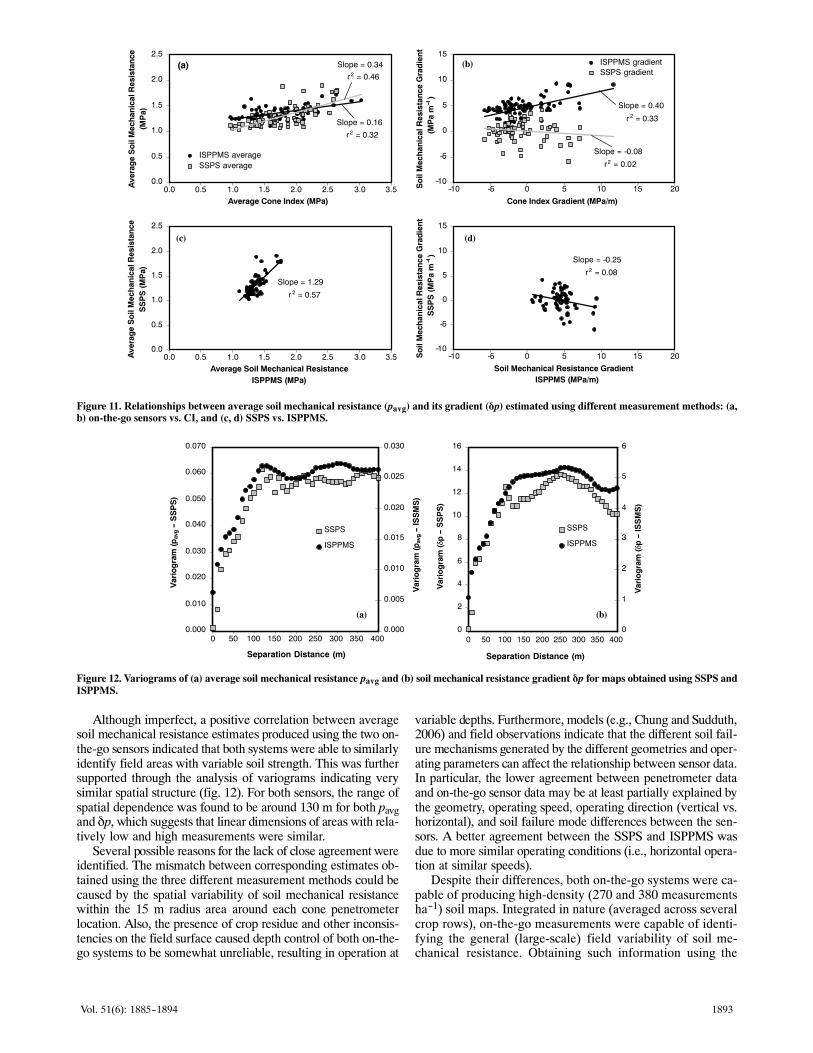
Figure 11. Relationships between average soil mechanical resistance (pavg) and its gradient (�p) estimated using different measurement methods: (a,b) on‐the‐go sensors vs. CI, and (c, d) SSPS vs. ISPPMS.

0.000

0.010

0.020

0.030

0.040

0.050

0.060

0.070

0 50 100 150 200 250 300 350 400

Separation Distance (m)

0.000

0.005

0.010

0.015

0.020

0.025

0.030

SSPS

ISPPMS

0

2

4

6

8

10

12

14

16

0 50 100 150 200 250 300 350 400

Separation Distance (m)

0

1

2

3

4

5

6

SSPS

ISPPMS

(a) (b)

Var

iog

ram

(pav

g -

SS

PS

)

Var

iog

ram

(pav

g -

ISS

MS

)

Var

iog

ram

(�p

- S

SP

S)

Var

iog

ram

(�p

- IS

SM

S)

Figure 12. Variograms of (a) average soil mechanical resistance pavg and (b) soil mechanical resistance gradient �p for maps obtained using SSPS andISPPMS.

Although imperfect, a positive correlation between averagesoil mechanical resistance estimates produced using the two on‐the‐go sensors indicated that both systems were able to similarlyidentify field areas with variable soil strength. This was furthersupported through the analysis of variograms indicating verysimilar spatial structure (fig. 12). For both sensors, the range ofspatial dependence was found to be around 130 m for both pavgand �p, which suggests that linear dimensions of areas with rela‐tively low and high measurements were similar.

Several possible reasons for the lack of close agreement wereidentified. The mismatch between corresponding estimates ob‐tained using the three different measurement methods could becaused by the spatial variability of soil mechanical resistancewithin the 15 m radius area around each cone penetrometerlocation. Also, the presence of crop residue and other inconsis‐tencies on the field surface caused depth control of both on‐the‐go systems to be somewhat unreliable, resulting in operation at

variable depths. Furthermore, models (e.g., Chung and Sudduth,2006) and field observations indicate that the different soil fail‐ure mechanisms generated by the different geometries and oper‐ating parameters can affect the relationship between sensor data.In particular, the lower agreement between penetrometer dataand on‐the‐go sensor data may be at least partially explained bythe geometry, operating speed, operating direction (vertical vs.horizontal), and soil failure mode differences between the sen‐sors. A better agreement between the SSPS and ISPPMS wasdue to more similar operating conditions (i.e., horizontal opera‐tion at similar speeds).

Despite their differences, both on‐the‐go systems were ca‐pable of producing high‐density (270 and 380 measurementsha-1) soil maps. Integrated in nature (averaged across severalcrop rows), on‐the‐go measurements were capable of identi‐fying the general (large‐scale) field variability of soil me‐chanical resistance. Obtaining such information using the

1894 TRANSACTIONS OF THE ASABE

cone penetrometer method would have been an extremely te‐dious process. The discrete‐depth resistance data obtained ona relatively coarse depth resolution with the SSPS directlyprovided five (four, discounting the unreliable 10 cm depth)layers of data that could be used to make management deci‐sions. Although correlated with each other, average soil me‐chanical resistance and its gradient, as provided by theISPPMS, represent two different data layers that can be usedto distinguish separate characteristics of the landscape(e.g.,�strong versus soft and uniform versus variable soil pro‐files). It is obvious that average soil mechanical resistancecan be used to identify potentially compacted field sites.

Although the soil mechanical resistance gradient providedby the ISPPMS represented soil strength changes with depthreasonably well for these Midwestern U.S. soils, its agronomicvalue is yet to be evaluated through follow‐up research. In dif‐ferent conditions where maximum compaction occurs deeper inthe soil profile (e.g., Coastal Plains soils of the SoutheasternU.S.), it might be necessary to increase the depth of mappingand/or return to a more complex model of the soil profile. Basedon the analysis in this article, it appears that spatially variablesoil productivity potential may have a similar or even greaterdegree of dependency on the way soil strength changes withdepth as on the overall magnitude of soil mechanical resistance.

CONCLUSIONSAn instrumented blade for mapping soil mechanical resist‐

ance using a linear depth effect model was developed and testedin both the laboratory and the field. The blade was a part of apreviously developed ISPPMS. Based on laboratory evaluation,strain gauges showed proper operation, and thus analytically de‐rived relationships between forces and strain values were used.During field testing, two different on‐the‐go soil sensing sys‐tems were compared. The two systems were run in the samefield and at the same time to reduce possible variations in fieldconditions. The instrumented blade for the ISPPMS determinedthe parameters of the linear depth effect model. The other sys‐tem (SSPS) used five horizontal prismatic tips at discretedepths. The correlations that were found between the ISPPMSand SSPS on‐the‐go sensor systems and the standard cone pe‐netrometer were marginal (r2�= 0.32 to 0.46, respectively, foraverage soil mechanical resistance estimates), while r2 = 0.57for the relationship between average soil mechanical resistancemeasured using the two on‐the‐go soil sensing systems. Gener‐ally, maps produced using the two sensors revealed the samestructure, as shown using variogram analysis. Some of the dif‐ferences were due in part to difficulties in obtaining data at thesame depth and field locations along with differences in sensorgeometry and operating conditions. This was especially truewhen comparisons were made between the on‐the‐go sensorsand the cone penetrometer. Depth gradients of soil mechanicalresistance obtained using the soil cone penetrometer and theISPPMS methods were correlated with r2 = 0.33. However, theagronomic value of this measurement in the top 30 cm of thesoil profile has yet to be determined.

REFERENCESAdamchuk, V. I., and P. T. Christenson. 2005. An integrated system for

mapping soil physical properties on‐the‐go: The mechanical sensingcomponent. In Precision Agriculture: Papers from the SixthEuropean Conference on Precision Agriculture, 449‐456. J.Stafford, ed. Wageningen, The Netherlands: Wageningen Academic.

Adamchuk, V. I., and P. T. Christenson. 2007. An instrumented bladesystem for mapping soil mechanical resistance represented as asecond‐order polynomial. Soil Tillage and Research 95(1): 76‐83.

Adamchuk, V. I., M. T. Morgan, and H. Sumali. 2001. Mapping ofspatial and vertical variation of soil mechanical resistance usinga linear pressure model. ASAE Paper No. 011019. St. Joseph,Mich.: ASAE.

Adamchuk, V. I., J. W. Hummel, M. T. Morgan, and S. K.Upadhyaya. 2004. On‐the‐go soil sensors for precisionagriculture. Computers and Electronics in Agric. 44(1): 71‐91.

Alihamsyah, T., E. G. Humphries, and C. G. Bowers. 1990. Atechnique for horizontal measurement of soil mechanicalimpedance. Trans. ASAE 33(1): 73‐77.

Andrade‐Sánchez, P., S. K. Upadhyaya, and B. M. Jenkins. 2007.Development, construction, and field evaluation of a soilcompaction profile sensor. Trans. ASABE 50(3): 719‐725.

ASABE Standards. 2006a. S313.3: Soil cone penetrometer. St.Joseph, Mich.: ASABE.

ASABE Standards. 2006b. EP542: Procedures for using andreporting data obtained with the soil cone penetrometer. St.Joseph, Mich.: ASABE.

Chung, S. O., and K. A. Sudduth. 2006. Soil failure models forvertically operating and horizontally operating strength sensors.Trans. ASABE 49(4): 851‐863.

Chung, S. O., K. A. Sudduth, and J. W. Hummel. 2006. Design andvalidation of an on‐the‐go soil strength profile sensor. Trans.ASABE 49(1): 5‐14.

Chung, S. O., K. A. Sudduth, C. Plouffe, and N. R. Kitchen. 2008.Soil bin and field tests of an on‐the‐go soil strength profilesensor. Trans. ASABE 51(1): 5‐18.

Dunn, P. F. 2005. Measurement and Data Analysis for Engineeringand Science. New York, N.Y.: McGraw‐Hill Higher Education.

Glancey, J. L., S. K. Upadhyaya, W. J. Chancellor, and J. W.Rumsey. 1989. An instrumented chisel for the study of soiltillage dynamics. Soil and Tillage Res. 14(1): 1‐24.

Gorucu, S., A. Khalilian, Y. J. Han, R. B. Dodd, and B. R. Smith.2006. An algorithm to determine the optimum tillage depth fromsoil penetrometer data in Coastal Plain soils. Applied Eng. inAgric. 22(5): 625‐631.

Hall, H. E., and R. L. Raper. 2005. Development and conceptualevaluation of an on‐the‐go soil strength measurement system.Trans. ASAE 48(2): 469‐477.

Hemmat, A., and V. I. Adamchuk. 2008. Sensor systems formeasuring soil compaction: Review and analysis. Computersand Electronics in Agric. 63(2): 89‐103

Horn, R., and T. Baumgartl. 2000. Dynamic properties of soils. InHandbook of Soil Science, A19‐A51. M. E. Sumner, ed. BocaRaton, Fla.: CRC Press.

Manor, G., R. L. Clark, D. E. Radcliffe, and G. W. Langdale. 1991.Soil cone index variability under fixed traffic tillage systems.Trans. ASAE 34(5): 1952‐1956.

McKyes, E. 1985. Soil physical properties. In Soil Cutting andTillage, 105‐123. New York, N.Y.: Elsevier Science.

Mouazen, A. M., H. Ramon, and J. De Baerdemaeker. 2003.Modelling compaction from on‐line measurement of soilproperties and sensor draught. Precision Agric. 4(2): 203‐212.

Owen, G. T., H. Drummond, L. Cobb, and R. J. Godwin. 1987. Aninstrumentation system for deep tillage research. Trans. ASAE30(6): 1578‐1582.

Raper, R. L., B. H. Washington, and J. D. Jarrell. 1999. Atractor‐mounted multiple‐probe soil cone penetrometer. AppliedEng. in Agric. 15(4): 287‐290.

Siefken, R. J., V. I. Adamchuk, D. E. Eisenhauer, and L. L.Bashford. 2005. Mapping soil mechanical resistance with amultiple blade system. Applied Eng. in Agric. 21(1): 15‐23.

Sudduth, K. A., N. R. Kitchen, G. A. Bollero, D. G. Bullock, andW. J. Wiebold. 2003. Comparison of electromagnetic inductionand direct sensing of soil electrical conductivity. Agronomy J.95(3): 472‐482.