v. bouyer et al- temperature profile calculation from emission spectroscopy measurements in...
TRANSCRIPT
8/3/2019 V. Bouyer et al- Temperature Profile Calculation From Emission Spectroscopy Measurements in Nitromethane Submi…
http://slidepdf.com/reader/full/v-bouyer-et-al-temperature-profile-calculation-from-emission-spectroscopy 1/10
8/3/2019 V. Bouyer et al- Temperature Profile Calculation From Emission Spectroscopy Measurements in Nitromethane Submi…
http://slidepdf.com/reader/full/v-bouyer-et-al-temperature-profile-calculation-from-emission-spectroscopy 2/10
The experiments consist in plane shock impacts on explosive targets at 8.6 GPa,under conditions of one-dimensional strain.A single stage powder gun propels the
projectile on the target at a velocity of 1940 m/s to initiate the detonation. The NM
is in a polyethylene chamber of 25 mmdepth, closed by a copper transfer plate4,5,6.An optical probe collects the thermalradiation emitted during the shock todetonation transition (SDT) through a lithiumfluoride window. This radiation istransmitted to the spectroscopy system by anoptical fiber. The light flux measured is theradiance emitted by the NM during the
propagation of shock and detonation waves.The spectroscopy device has been describedin previous papers5,6. The spectral and time
resolutions obtained are respectively 32 nm(16 channels) and 1 ns; the spectral rangestudied is 0.3-0.85 µm.
Complementary measurement techniquesare used: a polarization electrode records the
shock entrance, the superdetonation and thedetonation, piezo-electric pins measure theshock and detonation velocities.
RESULTS
We have performed several experiments of plate impacts at ~8.6 GPa on a 25 mm thick NM target (Table 1). V is the projectilevelocity, P is pressure, t1 is the formation of the superdetonation and t2 the formation of the strong detonation.
TABLE 1. CHARACTERISTICS OF
PLATE IMPACT SHOTS
Shot Nb. 76 1020 1045 2019
V(m/s) 1926 1937 1936 1946
P(GPa) 8.37 8.64 8.64 8.7
t1 1.7 1.65 1.38 1.6t2 2.36 2.15 1.84 2.15
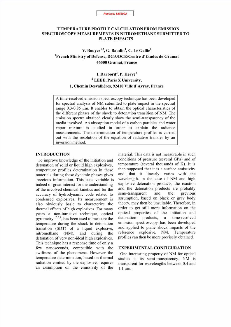
FIGURE 1. RADIANCE PROFILES OF SHOT 1020
Figure 1 represents the radiance signalsfor 16 wavelengths versus time obtainedduring shot 1020. Time resolution is 20 nsafter filtering through noise. Thesemeasurements, with the piezo-electric pinsand electrode signals clearly show the
different stages of the SDT as described byChaiken7.
Radiance temperature profiles have beencalculated with the Planck law (Figure 2).The true temperature is at least equal to themaximum radiance temperature.

8/3/2019 V. Bouyer et al- Temperature Profile Calculation From Emission Spectroscopy Measurements in Nitromethane Submi…
http://slidepdf.com/reader/full/v-bouyer-et-al-temperature-profile-calculation-from-emission-spectroscopy 3/10
FIGURE 2. RADIANCE TEMPERATURE OF SHOT 1020
Changes in radiance depending on
wavelength have been studied for varioustypical stages of the SDT (Figure 3).
From the formation of the superdetonation,a hollow appears between 0.65 and 0.75 µm.It remains until the end of the propagation of the detonation wave. This hollowcharacterizes semi-transparent optical
properties.
FIGURE 3. RADIANCE SPECTRA AT
DIFFERENT TIMES: a) after shock entrance(0.3 µs), b) before the superdetonation formation (1.2µs), c) superdetonation formation (1.65 µs), d) 1.9 µs,e) catch up of the shock wave (2.15 µs), f) strongdetonation (2.45 µs), g) overdriven steady statedetonation (3.8 to 4.4 µs). Radiance values wereaveraged around the given time value.
DISCUSSION
We studied the optical properties of thedifferent states of the SDT.
Shock entrance
The evolution of the signal emitted after shock entrance leads to conclude that theshock is transparent. The radiancetemperature after shock entrance is about2500 K. It has been also recorded by
pyrometry 4. It is not in good agreement withChaiken’s model that predicts a shock temperature of about 1000 K. Multipleshocks experiments performed at CEG leadto the same results8. We explain this hightemperature by local chemical reactions4 (hotspots) due to heterogeneities at the
impactor/explosive interface (Figure 4).
FIGURE 4. RADIATION EMITTEDDURING THE PROPAGATION OF THE
SHOCK
Sustained steady state detonation
The emitted radiation before the interactionwith the LiF window is constant. It could beexplained by a surface area emissivity of thedetonation front. But the radiancetemperature values during the detonation

8/3/2019 V. Bouyer et al- Temperature Profile Calculation From Emission Spectroscopy Measurements in Nitromethane Submi…
http://slidepdf.com/reader/full/v-bouyer-et-al-temperature-profile-calculation-from-emission-spectroscopy 4/10
propagation show a deviation of 500 K depending on the wavelengths (Figure 2).This implies that detonation products aresemi-transparent. The constant signal is morelikely due to the fact that the radiation comesfrom a small thickness behind the detonation
wave, remaining constant during the propagation (Figure 5). Detonation productsare called optically thick.
FIGURE 5. RADIATION EMITTED
DURING THE PROPAGATION OF THE
OVERDRIVEN DETONATION
We calculated the radiation emitted in thisconfiguration and compared it to theradiation emitted by the entire cell, by usingthe equation of radiative transfer (ERT).According to CJ theory, the temperature
profile behind the detonation front isconstant. Thus, for a sustained steady statedetonation, the ERT is 5:
)1)(()( )(0 0 x x K DeT L L−−−= λ
λ λ l (1)
Lλ is the radiance at wavelength λ, L0λ is the
black body radiance, T is the detonation products temperature, K λ is the absorptioncoefficient, xD and x0 are the detonation andimpactor/explosive interface positions, ℓ isthe cell depth.
Figure 6 shows that when K λ increases, theradiation emitted becomes constant and for the largest value of K λ, the radiation is the
same as the radiation emitted by a small layer of 5 mm thick behind the detonation front.
The detonation products are optically thick
but their emissivity )( 01 x x K De−−−= λ ε
is lower than 1 so they do not behave like a black body.
FIGURE 6. EFFECT OF K λ ON THE
RADIANCE
Superdetonation
The shock is transparent so we can measurethe radiation emitted by the superdetonationwave. BMI measurements performed at theCEG show that the laser beam crosses thereaction products thickness: they are semi-transparent. By focusing on the propagationof the superdetonation on Figure 1, we cansee that for wavelengths higher than 0.6 µm,the signal is constant whereas under 0.6 µm,it increases. In the first case, reaction
products behind the superdetonation behaveas steady state detonation products and in thesecond case, they are transparent. We can saythat reaction products are optically thick inthe spectral range 0.6-0.85 µm and optically
thin in the range 0.4-0.6 µm.
MODEL FOR THE ABSORPTION
COEFFICIENT
The results obtained on the optical properties of the reaction and detonation products lead us to try to find out whichspecies cause the hollow in the radiancespectra. In the visible range, only the carbonclusters and water vapor emit thermalradiation. Data on optical properties at high
pressures P and temperatures T does notexists. Our model is based on data at lower Pand T.
Carbon clusters
Clusters size has been estimated to 50 Å9.Volume fraction of carbon in detonation
products calculated with CHEETAH code is6%. Therefore, the particles are in adependent scattering regime that is difficult
8/3/2019 V. Bouyer et al- Temperature Profile Calculation From Emission Spectroscopy Measurements in Nitromethane Submi…
http://slidepdf.com/reader/full/v-bouyer-et-al-temperature-profile-calculation-from-emission-spectroscopy 5/10
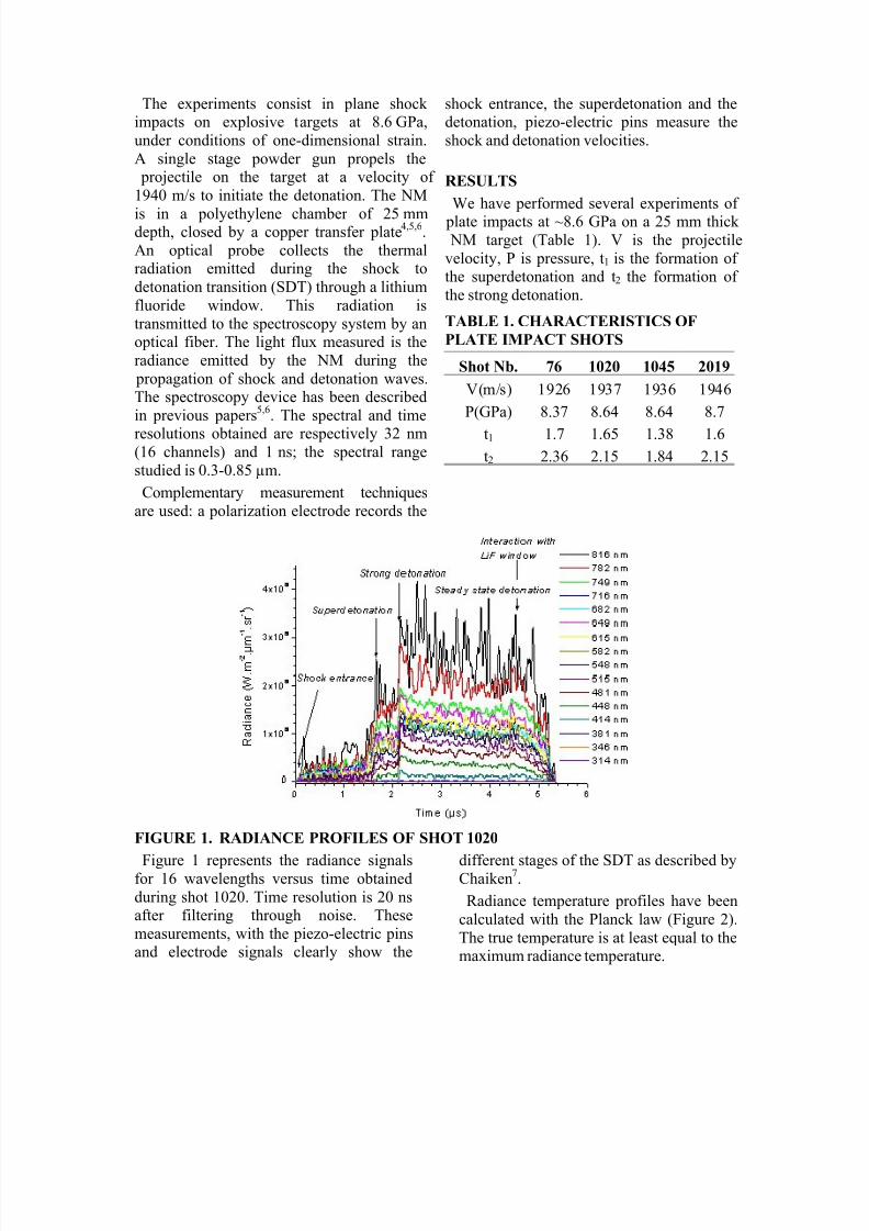
to calculate. We chose in a firstapproximation the independent scatteringregime that is Rayleigh scattering for small
particles size. In this case, scattering isnegligible and there is only absorption. Theabsorption coefficient of particles with
refractive index n-iχ, and volume fraction f v is 10:
λ χ χ
χ π λ
v f
nn
n K
22222 4)2(36
++−= (2)
Figure 7 shows K λ calculation for several f vvalues.
FIGURE 7. CALCULATION OF
K λ WITH EQUATION (2)
ERT of a scattering, emitting and absorbingmedium becomes ERT of an emitting and
absorbing medium so equation (1) can beused to calculate radiance emitted bydetonation products.
FIGURE 8. RADIANCE SPECTRA OF
CARBON CLUSTERS IN RAYLEIGH
SCATTERING REGIME
Figure 8 shows radiance values at theinteraction of the detonation wave with thewindow at 3600 K. More accurate
calculations show that we obtain the Planck curve at 3600 K for f v values higher than2.10-5.
Water vapor
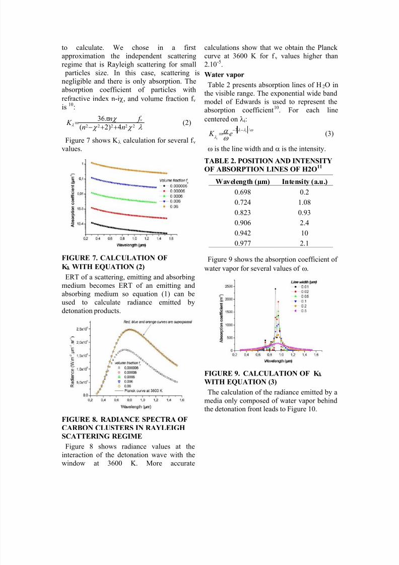
Table 2 presents absorption lines of H2O inthe visible range. The exponential wide bandmodel of Edwards is used to represent theabsorption coefficient10. For each linecentered on λi:
ω λ λ
λ ω α /2 i
i
e K −−
= (3)
ω is the line width and α is the intensity.
TABLE 2. POSITION AND INTENSITY
OF ABSORPTION LINES OF H2O11
Wavelength (µm) Intensity (a.u.)
0.698 0.2
0.724 1.08
0.823 0.93
0.906 2.4
0.942 10
0.977 2.1
Figure 9 shows the absorption coefficient of water vapor for several values of ω.
FIGURE 9. CALCULATION OF K λ
WITH EQUATION (3)
The calculation of the radiance emitted by amedia only composed of water vapor behindthe detonation front leads to Figure 10.

8/3/2019 V. Bouyer et al- Temperature Profile Calculation From Emission Spectroscopy Measurements in Nitromethane Submi…
http://slidepdf.com/reader/full/v-bouyer-et-al-temperature-profile-calculation-from-emission-spectroscopy 6/10
FIGURE 10. RADIANCE SPECTRA OF
WATER VAPOR
Water vapor and carbon clusters in
detonation products
We can now calculate the radiance of both
water vapor and carbon. The absorptioncoefficient of the mixture is the sum of theabsorption coefficient of water K λ
water andthe absorption coefficient of carbon K λ
carbon.If the volume fraction is too high, theradiance curves will fit the Planck curve at3600 K. If f v is lower than 2.10-5, it is thewater absorption coefficient that will give theshape of radiance spectra. The carbon willcreate a continuous background (Figure 11).
FIGURE 11. RADIANCE SPECTRA OF
WATER VAPOR AND CARBON
CLUSTERS
It has been difficult to fit the model with our emission spectroscopy measurements (seeshot 1045 on Figure 11). For lower wavelengths, the shapes are closed but thereis an intensity deviation and for wavelengthsof about 0.8 µm, our measurements seem to
fit to the water vapor line. Our model ismaybe too simple. It is likely that theRayleigh scattering independent model is notvalid. Moreover, we chose the simplestmodel for water vapor emission and we donot know the changes of the spectrum with
increasing pressures and temperatures.Moreover, the uncertainty on the volumefraction of carbon particles is high. With 6%of carbon, as calculated by CHEETAH code,the calculated radiance fit with Planck curveat the same temperature whereas we showed
previously that the medium was semi-transparent. The hypothesis of an emittingand absorbing medium is perhaps notadapted. Hence, the emitted radiation is notonly thermal radiation. In Gruzdkov andGupta works12, the emission spectrum
between 0.4 and 0.75 µm of NM shocked at16.7 GPa under a stepwise loading processhas been measured, and a peak appeared at0.65 µm. They explained it as luminescencefrom reaction products, maybe NO2. NO2 spectrum shows lines around 0.83 µm and
between 0.5 and 0.6 µm13. Fluorescence phenomena from NO2 or other species like N2 could take place at these wavelengths.
TEMPERATURE PROFILE
DETERMINATIONWe are presenting here a method to
determine temperature profiles during theSDT from the emission spectroscopymeasurements. It is based on the resolutionof the ERT by an inversion method.
FIGURE 12. EMMITING AND
ABSORBING MEDIUM
Given a semitransparent medium at atemperature T, with an absorption coefficientK λ and a thickness (x*-x0), the ERT is:
8/3/2019 V. Bouyer et al- Temperature Profile Calculation From Emission Spectroscopy Measurements in Nitromethane Submi…
http://slidepdf.com/reader/full/v-bouyer-et-al-temperature-profile-calculation-from-emission-spectroscopy 7/10
∫ −=*x
x(x)dxK )exp(xL(x*)L
0
λ 0λ λ
x'*x
xd
*x
x'(x)dxK (T)exp)L(x'K
0
λ 0λ
λ ∫
∫ −+ (4)
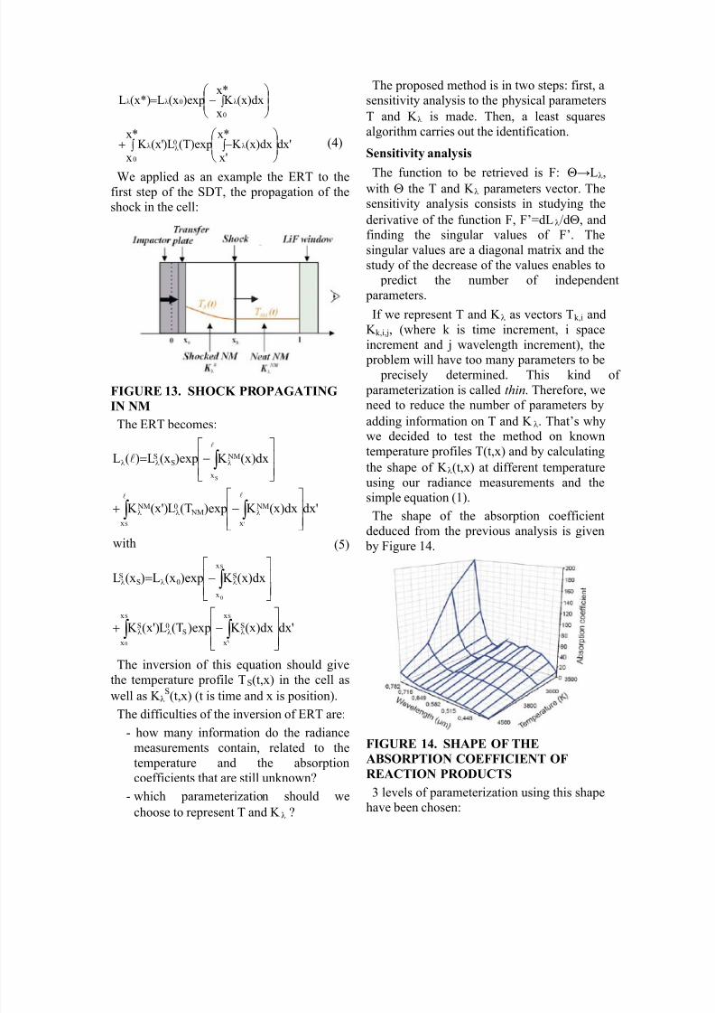
We applied as an example the ERT to thefirst step of the SDT, the propagation of theshock in the cell:
FIGURE 13. SHOCK PROPAGATING
IN NM
The ERT becomes:
'dxdx)x(K )expT(L')x(K
dx)x(K )expx(L)x(L
with
'dxdx)x(K )expT(L')x(K
dx)x(K )expx(L)(L
S
'
S
0
S
0
'S
S
x
'x
S
x
x
S0S
x
x
S0S
S
x
NM
x
NM0 NM
x
NMS
S
−+
−=
−+
−=
∫ ∫
∫
∫ ∫
∫
λλλ
λλλ
λλλ
λλλ
ll
l
l
(5)
The inversion of this equation should givethe temperature profile TS(t,x) in the cell aswell as K λ
S(t,x) (t is time and x is position).
The difficulties of the inversion of ERT are:- how many information do the radiance
measurements contain, related to thetemperature and the absorptioncoefficients that are still unknown?
- which parameterization should wechoose to represent T and K λ ?
The proposed method is in two steps: first, asensitivity analysis to the physical parametersT and K λ is made. Then, a least squaresalgorithm carries out the identification.
Sensitivity analysis
The function to be retrieved is F: Θ→
Lλ,with Θ the T and K λ parameters vector. Thesensitivity analysis consists in studying thederivative of the function F, F’=dLλ/dΘ, andfinding the singular values of F’. Thesingular values are a diagonal matrix and thestudy of the decrease of the values enables to
predict the number of independent parameters.
If we represent T and K λ as vectors Tk,i andK k,i,j, (where k is time increment, i spaceincrement and j wavelength increment), the
problem will have too many parameters to be precisely determined. This kind of parameterization is called thin. Therefore, weneed to reduce the number of parameters byadding information on T and K λ. That’s whywe decided to test the method on knowntemperature profiles T(t,x) and by calculatingthe shape of K λ(t,x) at different temperatureusing our radiance measurements and thesimple equation (1).
The shape of the absorption coefficient
deduced from the previous analysis is given by Figure 14.
FIGURE 14. SHAPE OF THE
ABSORPTION COEFFICIENT OF
REACTION PRODUCTS
3 levels of parameterization using this shapehave been chosen:
8/3/2019 V. Bouyer et al- Temperature Profile Calculation From Emission Spectroscopy Measurements in Nitromethane Submi…
http://slidepdf.com/reader/full/v-bouyer-et-al-temperature-profile-calculation-from-emission-spectroscopy 8/10
1. the values at the nodes of the grid areindependent,
2. the values in the grid are function of thevalues on the axis,
3. the shape is preserved, only the positionon the grid in Z axis changes.
The parameterization is a linear interpolation of the values of the grid. Ateach level, the number of parameters isreduced but each parameter contains moreinformation. This interpolation links the neat
NM state to the shocked NM state and theshocked state to the reacted explosive state asshown on Figure 15.
FIGURE 15. K λ LINEAR
INTERPOLATION
It is likely that this interpolation is notrepresenting the reality and we will have totake this into account when analyzing theresults.
The first studied temperature profiles are
presented Figure 16. The parameterization of the temperature is based on the shape of case1 and case 2 and is called red ( for reduced).
FIGURE 16. TEMPERATURE
PROFILES
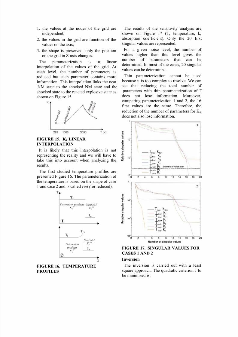
The results of the sensitivity analysis areshown on Figure 17 (T, temperature, k,absorption coefficient). Only the 20 firstsingular values are represented.
For a given noise level, the number of values higher than this level gives the
number of parameters that can bedetermined. In most of the cases, 20 singular values can be determined.
Thin parameterization cannot be used because it is too complex to resolve. We cansee that reducing the total number of
parameters with thin parameterization of Tdoes not lose information. Moreover,comparing parameterization 1 and 2, the 16first values are the same. Therefore, thereduction of the number of parameters for K λ
does not also lose information.
FIGURE 17. SINGULAR VALUES FOR
CASES 1 AND 2
Inversion
The inversion is carried out with a leastsquare approach. The quadratic criterion J to
be minimized is:

8/3/2019 V. Bouyer et al- Temperature Profile Calculation From Emission Spectroscopy Measurements in Nitromethane Submi…
http://slidepdf.com/reader/full/v-bouyer-et-al-temperature-profile-calculation-from-emission-spectroscopy 9/10
∑
−=
jk k j
k cal j
k mes jcal
L L L J
,
2,,
21)(
σ (6)
Lcal is radiance calculated with ERT, Lmes ismeasured radiance and σ stands for the noiseand relative errors of measurements. In the 2
cases presented here, Lmes
will be calculatedfrom temperature profiles of Figure 16.
The sensitivity analysis is a local analysis, performed around the searched value. A goodsensitivity does not guarantee that the
problem will be solved without finding localminima that are not the solution of the
problem. For example, Figure 18 shows thedrawing of the least square criterion J for case 1. Depending on the chosen
parameterization and on the initial point of the inversion algorithm, we can find localminimum (red curve).
FIGURE 18. EXAMPLE OF LOCAL
MINIMUM
The diagram on Figure 19 explains themethod used to find out inversion results for cases 1 and 2.
FIGURE 19. INVERSION METHOD OF
KNOWN TEMPERATURE PROFILES
The inversion method is validated if thedeviation between known temperature that isused to calculate radiance and the solution islow, i.e. low deviation between Lcal and Lmes.
Results of inversion for case 1 and case 2are given in Table 3.
TABLE 3. RESULTS OF INVERSION
Case 1
Parameterization Initial T(K)
TCJ (K)
d1 3000 3592
h3 3000 3601
h2 3601 3601
h1 3601 3600d1 4500 3600
h3 4500 3782
h2 3782 3600
h1 3600 3599
Case 2
Parameterization Initial T(K)
TCJ/TI (K)
d1 3250/2500 3251/2940
h3 3250/2500 3250/2810
h2 3250/2810 3486/3146h1 3486/3146 3486/3183
d1 4500/3250 4369/2877
h3 4500/3250 4500/3080
h2 4500/3080 4500/3168
h1 4500/3168 4500/3148
In case 1, TCJ=3600 K is the temperature to be determined.
In case 2, TCJ=3500 K, TI=3000 K .
We chose the reduced parameterization for
T. d1 corresponds to parameterization 1 of K λ. The parameterization h1, h2, and h3 arecoupled: we begin by using h3 (parameterization 3 of K λ). The results of h3 are used as initial point for h2 (parameterization 2 of K λ) and then, theresults of h2 are used as initial point for h1.

8/3/2019 V. Bouyer et al- Temperature Profile Calculation From Emission Spectroscopy Measurements in Nitromethane Submi…
http://slidepdf.com/reader/full/v-bouyer-et-al-temperature-profile-calculation-from-emission-spectroscopy 10/10
In case 1, the solution is the same as thesearched value 3600 K. Optimisation withh3,2,1 seems to give better results than with d1.But in case 2, if the initial point is to far fromthe searched values (3500/3000), theinversion solution does not give good results.
Therefore, the method is not yet efficient on profile 2 and on more complex profiles. Thedifficulty is linked to the parameterizationof T.
CONCLUSION
Time-resolved emission spectroscopy performed during the detonation of NM givesradiance measurements versus time between0.3 and 0.85 µm, with a 28 nm spectralresolution. Our results showed a
discontinuity between 0.65 and 0.75 µm inthe radiance profile, appearing from theformation of the superdetonation. This ischaracteristic of semi-transparency. Shocked
NM remains transparent. Reaction productsare optically thin in the range 0.4-0.6 µm andoptically thick in the range 0.6-0.85 µm.Detonation products are also optically thick in the visible range. The monochromaticabsorption coefficient of detonation productsdepends on wavelength and does notcorrespond to the emissivity of a black body.
An absorption model based on the emissionof carbon particles and water vapour is proposed. It is difficult to fit the model toemission measurements because of lack of data at high pressures and temperatures. Thedetermination of temperature profiles by aninversion method has been performed and iscurrently validated on the case of a steadystate detonation. The validation on theexperimental case is in progress.
ACKNOWLEDGEMENTS
The work described here was carried outwith financial support from DGA/SPNuc, for the interest of CEA. Each impact experiencewas performed at Physics of ExplosiveLaboratory at CEG with the assistance of ARES and Metrology staff.
G. Chavent and F. Clement of the ESTIMEteam at INRIA have developed the
mathematical solution to the inversionmethod.
REFERENCES
1. Kato Y., Mori N., Sakai H., Detonation
temperature of nitromethane and some solidhigh explosives, in 8th Symposium ondetonation, Albuquerque, NM, 1985, pp.558-566.2. Léal Crouzet B., Ph. D. Dissertation,University of Poitiers, France, 1998.3. Léal Crouzet B., Baudin G., Presles H.N.,Combustion and Flame 122, 463-473 (2000).4. Léal B, Baudin G., Goutelle J.C., PreslesH.N., An optical pyrometer for time resolvedtemperature measurements in detonationwave, 11th symposium on detonation, 1998,
pp. 353-361.5. Bouyer V., Baudin G., Le Gallic C.,Hervé P., Emission Spectroscopy Applied toShock to Detonation Transition in
Nitromethane, 12th APS Topical GroupMeeting on Shock Compression of Condensed Matter, Atlanta, 2001, pp. 1223-1226.6. Bouyer V., Time-resolved emissionspectroscopy measurements in nitromethanesubmitted to plate impacts, 52nd AeroballisticRange Association, Québec, 2001.
7. Chaiken R. F., The kinetic theory of detonation of high explosives, M.S Thesis,Polytechnic Inst. of Brooklyn, 1957.8. Baudin G., Serradeil R., Le Gallic C.,Bouinot P., Comportement sous choc dunitromethane, technical report, CEG, 2002.9. Winter N. W., Ree F. H., Stability of thegraphite and diamond phases of finite carbonclusters, 11th symposium on detonation,1998, pp. 480-489.10. M. F. Modest, Radiative Heat Transfer,Mc Graw-Hill International Editions, 1993.
11. Smith F. G. eds., Atmospheric propagation of radiation, SPIE OpticalEngineering Press, 1993.12. Gruzdkov Y. A., Gupta Y. M., J. Phys.Chem. A 102, 2322-2331 (1998).13. Herzberg G., Molecular spectra andmolecular structure, vol. III Electronicspectra and electronic structure of polyatomicmolecules, Masson, 1992.