uwhs ice core lesson plan - program on climate … · ice core lab 2 prior!knowledge!...

Ice Core Lab 1

Ice Core Lab

UWHS Climate Science

Unit 3: Natural Variability: Paleoclimate on Millennial Timescales

Ashley Maloney

Overview A solid understanding of timescales is crucial for any climate change discussion; this lab allows students to study changes in Earth’s atmospheric composition and temperature on millennial to orbital timescales. The Ice Core Lab is a fun hands-‐on supplement designed for the University of Washington in the High School Climate and Climate Change (ATMS 211) curriculum.

Focus Questions 1. How do we know about Earth’s climate before the instrumental record?

2. What is a proxy?

3. What timescale do ice cores capture?

4. What caused the cyclic changes in past CO2 and temperature?

5. What are the two main differences between natural CO2 variability during the past 800,000 years and recent CO2 levels recorded by modern instruments?

Learning Goals Students should be able . . .

1. To explain the difference between tectonic, orbital, and anthropogenic timescales.

2. To use marbles as a proxy for isotopes and make connections to scientific investigations using proxies, in particular isotope ratios of ice are a proxy for past temperatures.

3. To create and interpret student-‐generated and scientist-‐generated data of CO2 and ice isotopes naturally co-‐varying during glacial-‐interglacial cycles.

4. To explain using scientific data two key differences between anthropogenic CO2 and natural CO2 variability: rate and magnitude.

Background Ice cores come from every place in the world ice accumulates over time including tropical glaciers (see Kump et al. chapter 6 pp. 113 – 117 for glacier and ice sheet information). The most famous ice cores are from the Greenland and Antarctic ice sheets. The longest and most robust records of atmospheric CO2 are from Antarctica (northern hemisphere dust causes chemical changes in the gas bubbles in Greenland ice cores). The longest ice core record collected by scientists extends back 800,000 years. The CO2 record comes from gas in the ice: atmospheric gases diffuse into the top layer of snow. As the top layer (“firn”) densifies it becomes ice, trapping the gas in bubbles. Old ice far below the surface has bubbles that were trapped thousands of years ago -‐ leaving scientists with a way to directly measure Earth’s past atmosphere. Less straightforward is the temperature record inferred from the stable hydrogen or oxygen isotopic composition of the water molecules that make up ice. Variations in temperature through time cause variations in the deuterium/hydrogen (D/H) ratios in ice. Isotope data is expressed using “delta” (δ) notation. Very negative δDice values represent colder temperatures (glacial periods) and less negative values are found during warmer climate conditions (interglacial periods).

Grade Level 9-12 Time Required 2 weeks Preparation • 1 week to order/gather materials • 3-6 hours to become familiar with

data and plan • 15 minutes/day for ~one week 1-3 hours Class Time • 5 minute pre survey • 0.5 - 1 hour lab introduction • 10min proxy exercise • 0.5 - 1 hours to gather data from ice

cores, assemble class data, and plot in Excel

• 0.5 - 1 hour to plot extended record in Excel and examine trends

• 5 minute post survey Materials Needed Reference textbook: Kump LR, Kasting JF, Crane GC (2010) The Earth System. Pearson To make ice cores • Freezer space for five 1ft tall tubes • Hacksaw or pipe-cutter to cut

acrylic tube into 5 sections • Order plastic tube ($17.22 for 6ft) at

http://www.usplastic.com/catalog/item.aspx?itemid=32520&catid=440

• Order endcaps ($1.85 for 5 caps) at http://www.usplastic.com/catalog/item.aspx?itemid=29228&catid=841

• Electrical tape to attach endcaps • Waterproof sharpie • Green, purple, and orange marbles • Write-in-the-rain paper To dissect ice cores • Large cutting board(s) or dish bins • Hacksaw(s) • Hammer and chisel(s) • Hot water • Strainer • 10-20 dish towels • 20 small Dixie cups • Work gloves and safety goggles

Ice Core Lab 2

Prior Knowledge The lab is intended for students who already know about CO2 as a greenhouse gas. Students are likely familiar with some paleoproxies. Ice cores, tree rings, speleothems (cave deposits), marine sediments, lake sediments and coral skeletons all store information about the past. Earth’s climate was quite different during the Last Glacial Maximum about 20,000 years ago when ice sheets were at their full extent. Sea levels were about 120 meters (400ft) lower, much of the Northern Hemisphere was covered in ice sheets, wooly mammoths, giant sloths, and saber-‐toothed cats still roamed, and the climate was cooler and drier.

Procedures PRE LAB: MAKING ICE CORES (allow 1-‐2 weeks for preparations)

This lab is designed for five student groups (but can accommodate six). It takes a week to assemble all the material and 4 days to make the ice cores since each layer needs a day to freeze. You will make 20,000 years worth of an ice core in 5 sections. Each section has four layers and every layer represents 1000 years. The CO2 and temperature proxy data you need for each layer are on the first sheet of the Excel file (called “Making Ice Cores”) and shown in two figures below. The second sheet of the Excel file (called “Understanding the Data”) explains how the raw data were manipulated to create the twenty CO2 and twenty temperature proxy data points needed for making the ice core. Assemble all materials and plan out the ingredients for each layer for the 5 cores. First label all 5 tube-‐sections with dates using electrical tape and sharpie. For instance, the first tube section for Group #1 should have four layers labeled 0-‐1000 yrBP, 1000-‐2000 yrBP, and so on. Tape the end cap on the tube and pour in ~½ cup of water (it is better to add more rather than less water so that students have enough ice to hold on to during the dissections). Drop in a piece of Write in the Rain paper with the CO2 concentration written on it. Add the marbles that represent the hydrogen isotope data (marbles work best so they all settle in the same place whereas beads or beans tend to float and this can led to students attributing data to the wrong layer). After water and marbles are added, drop in a piece of wax paper cut to fit the diameter of the tube (this step is optional so it isn’t too difficult for students to separate the ice layers), and then place in freezer for a day. Make sure the first layer is completely frozen before adding the next layer or layers will mix and students will get confused. BE SURE TO ADD THE CORRECT DATA TO THE CORRECT LAYER.

Teacher Orientation This lab is based on the longest ice core record available: EPICA Dome C, Antarctica (record shown on right -‐ figure 1-‐10 p.15 of Kump et al.). Since it is impractical to make the entire ice core, the homemade ice cores represent just the last 20,000 years. There are ~10 CO2 and ~80 isotope measurements for each 1000 years of ice so CO2 concentrations and isotope date are averaged every 1000 years for the purposes of this lab. Find all data required for this lab on six tabs of an Excel spreadsheet (“UWHS ICE CORE LESSON DATA”). Study this lesson plan along with the Excel spreadsheet to learn how to run the lab. Years Before Present (yrBP) means years before 1950 since the radiocarbon standard was set to a date proceeding excessive bomb carbon. CO2 units are PPMV = parts per million volume which reflects the concentration of CO2 in an air sample.

Ice Core Lab 3

INTRODUCING THE LAB (30-‐60min discussion)

PRE SURVEY: Please have each student fill out the Pre Lab Survey (Page 9.)

The point of this introduction is to expose students to different timescales -‐ they should be able to explain the difference between tectonic/geologic, millennial to orbital, and anthropogenic timescales. Additionally, this introduction should answer any questions students may have about ice cores. Discuss how difficult it is to get a real ice core so that they appreciate how much work went into obtaining the original data.

PRIOR KNOWEDGE: Probe the class to find out what they already know about past climate. How do scientists know about ancient CO2? How are we supposed to know what temperatures were like before thermometers were invented? When were thermometers invented anyways? When was the instrument that measures present day atmospheric CO2 levels invented? Who invented it? Revisit the Keeling curve (http://scrippsco2.ucsd.edu/program_history/keeling_curve_lessons.html). Why do we care about past climate?

TIMESCALES: One of the most important, fundamental concepts about paleoclimate is timescales. Before diving into the millennial to orbital timescale that this lab is devoted to, review changes in temperature and CO2 that occur on other timescales: diurnal, seasonal, decadal, anthropogenic, millennial, geologic/tectonic. Have students visit the NOAA Paleoclimatology TimeLine http://www.ncdc.noaa.gov/paleo/ctl/index.html. Check out Earth maps from different periods in Earth history at http://cpgeosystems.com/mollglobe.html. Chapter 12 (p.233) in Kump et al. is devoted to long-‐term climate variability, which is controlled by very different processes (for example silicate weathering in Chapter 8, p.159) than the climatic variations that occur on millennial or orbital timescales. Earth is presently in an “Ice Age” (albeit an interglacial within the ice age) because there are large permanent ice sheets in both Polar Regions. Other Ice Ages are rare and occurred millions of years ago (geologic timescale) and we can’t use ice cores to study ancient ice ages because that ice is long gone. The long-‐term climate record is inferred from deep-‐sea sediment cores (until about 200 million years ago), continental rocks, and geologic deposits (pp. 240 – 252 Kump et al.).

FIELD WORK: Engaging the students in an animated discussion about going to the field to obtain ice cores and then guessing what the data will show is a good way to introduce the lab. Some questions you might ask: It is time to plan an expedition to Antarctica! What does it take to plan a scientific field expedition? Who pays for it? Who is in charge of the logistics? What tools do we need? What clothes do we need? How do we get ice cores back to the lab? Where do we store them once they are here? How are we going to divvy up the ice to measure all the different parameters (CO2, N2O, CH4, stable isotopes, snow accumulation, grain radius, dust, conductivity, ionic chemistry…)? What do you think CO2 levels looked like in the past? Has temperature been constant during the last 20,000 years? The last 800,000 years? How do you think it has varied?

WHAT IS THE TEMPERATURE PROXY? (20-‐40min discussion/lesson and activity)

The point of this activity is to become familiar with how hydrogen isotopes are used as a proxy for temperature – and how marbles are a proxy for isotopes!

DISCUSSION/LESSON: A proxy is a substitute for an actual measurement. CO2 data from ice cores is not proxy data because the CO2 record is derived from measurements of ancient air bubbles trapped in ice. However, ice core temperature data is derived from a proxy. Isotope measurements of the water molecules that make up the ice reveal past temperature changes. Isotopes are identical atoms with different masses due to different amounts of neutrons (see p. 15 and p. 274 in Kump et al. for the basics). There are two stable hydrogen isotopes: “protium” which is normal hydrogen with one electron, one proton, and zero neutrons, and “deuterium” which is the rare stable hydrogen isotope with one electron, one proton, and one neutron. The ratio of heavy to light hydrogen isotopes in ice cores change when temperature changes: during colder glacial periods the ratios are lighter and during warmer interglacial periods the ratios are heavier. This is because rare, heavy isotopes generally prefer to remain in ocean water -‐ a more energetically stable state than water vapor and when they do leave the surface ocean, the heavy isotopes prefer to rain out of the atmosphere, leaving the lighter isotopes in the atmosphere to travel to the poles. During a cold glacial period, the equator to pole temperature gradient is large and very few heavy hydrogen isotopes make it to the poles because they rain out very soon after leaving the ocean surface. During a warm interglacial however, there is more energy in the Earth system and the equator to pole temperature gradient is relatively small which leads to more water molecules with a heavy isotope traveling to the pole.

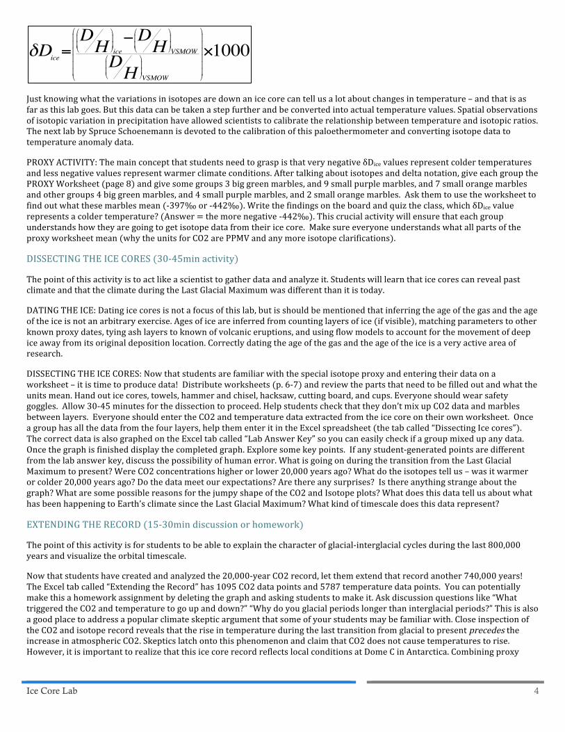
ISOTOPE DATA NOTATION: Because deuterium is very rare, hydrogen isotope ratios are very small numbers and they need to be related to a standard. Thus isotope data is expressed in delta (δ) notation (the relative deviation of a sample’s isotopic ratio compared to the isotopic ratio of the standard VSMOW) with units in per mil (‰). Ice core “delta” values are negative because the D/H ratio of the ice core sample is compared to VSMOW. The “delta” value of mean ocean water (VSMOW) is zero. The ocean has more deuterium than most natural substances – so most samples have a negative value according to “delta” notation because they are depleted in deuterium relative to the standard. The units are per mil (‰) so that the numbers are not much less than unity.

Ice Core Lab 4

Just knowing what the variations in isotopes are down an ice core can tell us a lot about changes in temperature – and that is as far as this lab goes. But this data can be taken a step further and be converted into actual temperature values. Spatial observations of isotopic variation in precipitation have allowed scientists to calibrate the relationship between temperature and isotopic ratios. The next lab by Spruce Schoenemann is devoted to the calibration of this paloethermometer and converting isotope data to temperature anomaly data.

PROXY ACTIVITY: The main concept that students need to grasp is that very negative δDice values represent colder temperatures and less negative values represent warmer climate conditions. After talking about isotopes and delta notation, give each group the PROXY Worksheet (page 8) and give some groups 3 big green marbles, and 9 small purple marbles, and 7 small orange marbles and other groups 4 big green marbles, and 4 small purple marbles, and 2 small orange marbles. Ask them to use the worksheet to find out what these marbles mean (-‐397‰ or -‐442‰). Write the findings on the board and quiz the class, which δDice value represents a colder temperature? (Answer = the more negative -‐442‰). This crucial activity will ensure that each group understands how they are going to get isotope data from their ice core. Make sure everyone understands what all parts of the proxy worksheet mean (why the units for CO2 are PPMV and any more isotope clarifications).

DISSECTING THE ICE CORES (30-‐45min activity)

The point of this activity is to act like a scientist to gather data and analyze it. Students will learn that ice cores can reveal past climate and that the climate during the Last Glacial Maximum was different than it is today.

DATING THE ICE: Dating ice cores is not a focus of this lab, but is should be mentioned that inferring the age of the gas and the age of the ice is not an arbitrary exercise. Ages of ice are inferred from counting layers of ice (if visible), matching parameters to other known proxy dates, tying ash layers to known of volcanic eruptions, and using flow models to account for the movement of deep ice away from its original deposition location. Correctly dating the age of the gas and the age of the ice is a very active area of research.

DISSECTING THE ICE CORES: Now that students are familiar with the special isotope proxy and entering their data on a worksheet – it is time to produce data! Distribute worksheets (p. 6-‐7) and review the parts that need to be filled out and what the units mean. Hand out ice cores, towels, hammer and chisel, hacksaw, cutting board, and cups. Everyone should wear safety goggles. Allow 30-‐45 minutes for the dissection to proceed. Help students check that they don’t mix up CO2 data and marbles between layers. Everyone should enter the CO2 and temperature data extracted from the ice core on their own worksheet. Once a group has all the data from the four layers, help them enter it in the Excel spreadsheet (the tab called “Dissecting Ice cores”). The correct data is also graphed on the Excel tab called “Lab Answer Key” so you can easily check if a group mixed up any data. Once the graph is finished display the completed graph. Explore some key points. If any student-‐generated points are different from the lab answer key, discuss the possibility of human error. What is going on during the transition from the Last Glacial Maximum to present? Were CO2 concentrations higher or lower 20,000 years ago? What do the isotopes tell us – was it warmer or colder 20,000 years ago? Do the data meet our expectations? Are there any surprises? Is there anything strange about the graph? What are some possible reasons for the jumpy shape of the CO2 and Isotope plots? What does this data tell us about what has been happening to Earth’s climate since the Last Glacial Maximum? What kind of timescale does this data represent?

EXTENDING THE RECORD (15-‐30min discussion or homework)

The point of this activity is for students to be able to explain the character of glacial-‐interglacial cycles during the last 800,000 years and visualize the orbital timescale.

Now that students have created and analyzed the 20,000-‐year CO2 record, let them extend that record another 740,000 years! The Excel tab called “Extending the Record” has 1095 CO2 data points and 5787 temperature data points. You can potentially make this a homework assignment by deleting the graph and asking students to make it. Ask discussion questions like “What triggered the CO2 and temperature to go up and down?” “Why do you glacial periods longer than interglacial periods?” This is also a good place to address a popular climate skeptic argument that some of your students may be familiar with. Close inspection of the CO2 and isotope record reveals that the rise in temperature during the last transition from glacial to present precedes the increase in atmospheric CO2. Skeptics latch onto this phenomenon and claim that CO2 does not cause temperatures to rise. However, it is important to realize that this ice core record reflects local conditions at Dome C in Antarctica. Combining proxy

δDice=DH!

"

##

$

%

&&ice−DH

!

"

##

$

%

&&VSMOW

DH!

"

##

$

%

&&VSMOW

!

"

######

$

%

&&&&&&

×1000

Ice Core Lab 5

records from around the world (Shakun et al. 2012) reveals that on a global scale CO2 increases before global temperatures, while local conditions in Antarctica stray from the global mean. Potential reasons for the local differences relate to the timing of changes in ocean circulation, sea ice cover, permafrost and terrestrial plant growth, and albedo – all of which were experiencing major changes during the transition. Regardless of the mechanism, the main point is that the timing of CO2 and temperature records from the Antarctic ice core represent local, not global, conditions and can therefore not be used as evidence to suggest that CO2 is not a cause for changes in temperatures. Also – it is possible that ice core ages and gas ages are not perfectly reconstructed.

ADDING MODERN DATA TO THE RECORD (30-‐60min discussion or homework)

The point of this activity is to explain using scientific data two key differences between anthropogenic CO2 and natural CO2 variability: rate and magnitude.

How is natural variability different than anthropogenic climate change? The Excel tab called “Add Instrumental Data” includes two new data sets: the modern record from CO2 measurements made for the past 53 years, and a different ice core from Law Dome to connect the gap between the instrumental record and the Dome C ice core. There are two key points to this activity. First: observe the scale of human-‐caused CO2 change. Natural CO2 variability during the past 800,000 years has been between 180 and 300 ppmv. Humans have added 90 ppm to the atmosphere, which is an additional 75% on top the natural signal. Second: notice the rate – it may help to change the scale on the x-‐axis or plot the best fit lines that describe CO2 increase at glacial-‐interglacial transitions and compare those slopes to recent CO2 increase. It took humans only 100 years to cause this change while it takes the natural cycle 10000 years to add 100ppmv CO2 to the atmosphere. This is one reason why it is important to know about Earth’s past climate. Without this knowledge we would have no baseline to compare human impact on climate. Have students watch this instructive video on past CO2 fluctuations a few times: http://www.esrl.noaa.gov/gmd/ccgg/trends/history.html

POST SURVEY: Please have each student fill out the Post Lab Survey (Page 10 and 11) and mail both surveys to: Ashley Maloney, School of Oceanography, Box 355351, University of Washington, Seattle WA 98195, (206) 685 9090, [email protected]

References Textbook: Kump LR, Kasting JF, Crane GC (2010) The Earth System. Pearson Shakun, JD, Clark PU, He F, Marcott SA, Mix AC, Liu Z, Otto-Bliesner B, Schmittner A, Bard E (2012) Global warming preceded by increasing carbon dioxide concentrations during the last deglaciation. Nature 484 pp. 49-56 (http://people.oregonstate.edu/~schmita2/pdf/S/shakun12nat.pdf)

Additional Resources • ICE CORES • Similar data analysis activities based on the 400,000 year Vostok, Antarctica record

- http://serc.carleton.edu/usingdata/datasheets/Vostok_IceCore.html - http://serc.carleton.edu/introgeo/mathstatmodels/examples/Vostok.html - http://eesc.columbia.edu/courses/ees/climate/labs/vostok/

• Another approach to making ice cores that study weather events during a winter season from NASA’s Education Student Observation Network at http://www.nasa.gov/audience/foreducators/son/winter/snow_ice/students/F_Snow_and_Ice_Students.html

• PALEOCLIMATE • Timescales: NOAA timeline http://www.ncdc.noaa.gov/paleo/ctl/index.html

• Paleoclimate animations http://emvc.geol.ucsb.edu/1_DownloadPage/Download_Page.html

• Paleoclimatology overview http://serc.carleton.edu/microbelife/topics/proxies/paleoclimate.html

• NOAA Paleoclimatology data portal http://www.ncdc.noaa.gov/paleo/paleo.html

• What’s the connection between low sea level and big ice sheets? Deep Sea Paleoclimate http://oceanexplorer.noaa.gov/explorations/05stepstones/background/paleoclimate/paleoclimate.html

• Where are ice cores stored? http://nicl.usgs.gov/about.htm

• Antarctic marine sediment core lesson plan http://serc.carleton.edu/eet/cores/index.html

• MILANKOVITCH CYCLES • Lesson: http://www.sciencecourseware.org/eec/GlobalWarming/Tutorials/Milankovitch/

• Visualization: http://highered.mcgraw-hill.com/sites/0073369365/student_view0/chapter16/milankovitch_cycles.html

• Interactive: http://umassk12.net/ipy/materials/2010Summer/cycle.html

Ice Core Lab 6

ICE CORE DATA Worksheet You have 4 layers of ice. Each layer of ice represents 1000 years of accumulation. There are 3 pieces of information associated with each layer that you need to record on this sheet: a. AGE b. CO2 c. ISOTOPE PROXY DATA. The age of each layer is found on a label on the outside of the core – CAREFUL don’t mix up the top and bottom of the core! CO2 concentration data can be found on small piece of paper and isotope data (used by scientists as a proxy for temperature) is represented by a special proxy (colored marbles).

FIRST DATA POINT

a. AGE RANGE (Years Before Present)= _____________________

b. CO2 (1000-‐year average concentration of CO2) = __________________________(PPMV)

c. Temperature Proxy (deuterium/hydrogen ratio of ice relative to the standard) δD = -‐ __________ __________ (‰)

SECOND DATA POINT




# of green marbles = # of purple marbles = # of orange marbles =


Ice Core Lab 7

THIRD DATA POINT




FOURTH DATA POINT






Ice Core Lab 8

PROXY Worksheet In this exercise colored marbles are a proxy for isotope data expressed in delta notation. Because we don’t have access to a mass spectrometer this lab uses a proxy (marbles) for a proxy (isotopes)! The ratio of heavy vs. light (D/H) hydrogen isotopes in the water molecules that make up ice varies along with changes in local temperature. Deuterium is so rare that the D/H ratio of ice is a very small number and isotope ratios of environmental samples need to be compared to a standard to make sense, therefore isotope data is expressed using delta notation. δD values of hydrogen isotopes in ice cores are three digit negative values. Large green marbles represent the 100s digit, small purple marbles represent the 10s digit, and small orange marble represent the 1s digit.

Instructions:

1. You will be given a handful of beads.

2. Place the colored marbles in the matching square below.

3. Write down the number of beads in each colored box.

4. Translate the marbles into a negative number such as and write your answer here

δD = __________ __________ (‰)

-‐Why is the “delta” value negative? Because the D/H ratio of the any sample is always compared to a standard for reference. For water isotopes, the standard is Vienna Standard Mean Ocean Water (VSMOW). The “delta” δ value of mean ocean water (VSMOW) is zero. The ocean has more deuterium than most natural substances – so most samples have a negative value according to “delta” notation because they are depleted in deuterium relative to the standard.

-‐Why are the units per mil (‰)? The answer is simple! Convenience (otherwise we would have to work with very small numbers, which is annoying).

δDice=DH!

"

##

$

%

&&ice−DH

!

"

##

$

%

&&VSMOW

DH!

"

##

$

%

&&VSMOW

!

"

######

$

%

&&&&&&

×1000

# of green marbles =

# of purple marbles =

# of orange marbles =

Ice Core Lab 9

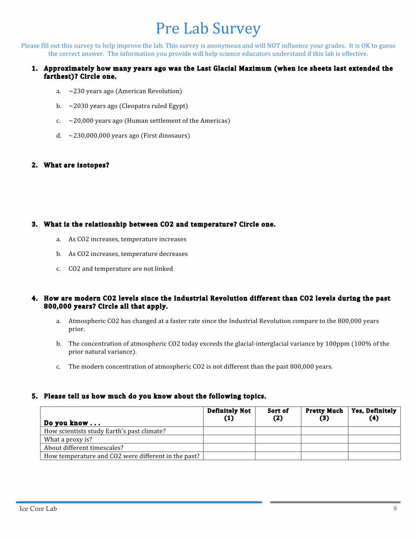
Pre Lab Survey Please fill out this survey to help improve the lab. This survey is anonymous and will NOT influence your grades. It is OK to guess

the correct answer. The information you provide will help science educators understand if this lab is effective.

1 . Approximately how many years ago was the Last Glacial Maximum (when ice sheets last extended the farthest)? Circle one.

a. ~230 years ago (American Revolution)

b. ~2030 years ago (Cleopatra ruled Egypt)

c. ~20,000 years ago (Human settlement of the Americas)

d. ~230,000,000 years ago (First dinosaurs)

2 . What are isotopes?

3 . What is the relationship between CO2 and temperature? Circle one.

a. As CO2 increases, temperature increases

b. As CO2 increases, temperature decreases

c. CO2 and temperature are not linked

4. How are modern CO2 levels since the Industrial Revolution different than CO2 levels during the past 800,000 years? Circle all that apply.

a. Atmospheric CO2 has changed at a faster rate since the Industrial Revolution compare to the 800,000 years prior.

b. The concentration of atmospheric CO2 today exceeds the glacial-‐interglacial variance by 100ppm (100% of the prior natural variance).

c. The modern concentration of atmospheric CO2 is not different than the past 800,000 years.

5 . Please tell us how much do you know about the following topics.

Do you know . . .

Definitely Not (1)

Sort of (2)

Pretty Much (3)

Yes, Definitely (4)

How scientists study Earth’s past climate? What a proxy is? About different timescales? How temperature and CO2 were different in the past?

Ice Core Lab 10

Post Lab Survey (Front and Back!) Please fill out this survey to help improve the lab. This survey is anonymous and will NOT influence your grades. It is OK to guess

the correct answer. The information you provide will help science educators understand if this lab is effective.

1 . Approximately how many years ago was the Last Glacial Maximum (when ice sheets last extended the farthest)? Circle one.

a. ~230 years ago (American Revolution)

b. ~2030 years ago (Cleopatra ruled Egypt)

c. ~20,000 years ago (Human settlement of the Americas)

d. ~230,000,000 years ago (First dinosaurs)

2 . What are isotopes?

3 . Which δDice value represents a colder temperature? Circle one.

a. δDice = -‐442‰

b. δDice = -‐397‰

4. What is the relationship between CO2 and temperature? Circle one.

a. As CO2 increases, temperature increases

b. As CO2 increases, temperature decreases

c. CO2 and temperature are not linked

5. How are modern CO2 levels since the Industrial Revolution different than CO2 levels during the past 800,000 years? Circle all that apply.

a. Atmospheric CO2 has changed at a faster rate since the Industrial Revolution compare to the 800,000 years prior.

b. The concentration of atmospheric CO2 today exceeds the glacial-‐interglacial variance by 100ppm (100% of the prior natural variance).

c. The modern concentration of atmospheric CO2 is not different than the past 800,000 years.

6 . Please tell us how much do you know about the following topics.

Do you know . . .

Definitely Not (1)

Sort of (2)

Pretty Much (3)

Yes, Definitely (4)

How scientists study Earth’s past climate? What a proxy is? About different timescales? How temperature and CO2 were different in the past?

Ice Core Lab 11

7. What would you say was the most important thing you learned from this lab?

8 . Is there anything about the lab you found confusing?

Thanks for filling out this survey!

uwhs ice core lesson plan - program on climate … · ice core lab 2 prior!knowledge!...

Documents