UvA-DARE is a service provided by the library of the University of Amsterdam (http://dare.uva.nl)

UvA-DARE (Digital Academic Repository)

Collateral and the limits of debt capacity: theory and evidence

Giambona, E.; Mello, A.S.; Riddiough, T.

Link to publication

Citation for published version (APA):Giambona, E., Mello, A. S., & Riddiough, T. (2012). Collateral and the limits of debt capacity: theory andevidence. Amsterdam: Universiteit van Amsterdam.

General rightsIt is not permitted to download or to forward/distribute the text or part of it without the consent of the author(s) and/or copyright holder(s),other than for strictly personal, individual use, unless the work is under an open content license (like Creative Commons).

Disclaimer/Complaints regulationsIf you believe that digital publication of certain material infringes any of your rights or (privacy) interests, please let the Library know, statingyour reasons. In case of a legitimate complaint, the Library will make the material inaccessible and/or remove it from the website. Please Askthe Library: http://uba.uva.nl/en/contact, or a letter to: Library of the University of Amsterdam, Secretariat, Singel 425, 1012 WP Amsterdam,The Netherlands. You will be contacted as soon as possible.

Download date: 26 Aug 2018

Electronic copy available at: http://ssrn.com/abstract=2039253

Collateral and the Limits of Debt Capacity: Theory and Evidence*

Erasmo Giambona

University of Amsterdam

e.giambona@uva.nl

Antonio S. Mello

University of Wisconsin

amello@bus.wisc.edu

Timothy Riddiough

University of Wisconsin

triddiough@bus.wisc.edu

This version: April 12, 2012

Abstract

This paper considers how collateral is used to finance a going concern, and demonstrates with theory and evidence

that there are effective limits to debt capacity and the kinds of claims that are issued to deploy that debt capacity.

The theory shows that firms with (unobservably) better quality collateral optimally pledge an unused portion of that

collateral to finance new investment opportunities with unsecured debt, while firms endowed with lower quality

collateral use project-specific secured debt. Better quality firms must also commit to maintaining an equity cushion

to separate themselves from lesser quality firms, implying lower relative leverage and greater uncommitted cash

flow from operations with which to meet debt service requirements. The fundamental empirical prediction derived

from our model is that a firm’s financing choice, as it relates to asset quality, reveals information about firm value.

To establish this link empirically, we rely on a natural experiment from the listed-property firm industry. Housing

property-firms had access to Fannie Mae-Freddie Mac secured debt financing during the peak of the 1998 Russian

crisis (but not other financing options), whereas Non-Housing firms were shut out of all financing channels.

Empirical evidence indicates that, consistent with our theory, better quality Housing firms migrated from the

unsecured debt market into the secured debt market during a time of high equity issuance costs, thus raising the

average revealed asset quality of firms in the pool of secured debt issuers. We rely on a series of falsification tests to

rule out alternative explanations for our empirical findings.

.

*Send correspondence to: Erasmo Giambona, Finance Group, University of Amsterdam, 1018 WB Amsterdam, The Netherlands.

E-mail: e.giambona@uva.nl. Phone: +31 20 525 5321. We appreciate comments from Heitor Almeida, Murillo Campello, Piet

Eichholtz, John Geanakoplos, John Harding, Jay Hartzell, Dwight Jaffee, Igor Makarov, Alan Moreira, Justin Murfin, Frank

Nothaft, Joe Pagliari, Mark Parrell, Florian Peters, Adriano Rampini, Steve Ross, David Shulman, Matthew Spiegel, Bob Van

Order, Nancy Wallace, Tony Yezer. We also thank seminar participants at Duisenberg School of Finance, European Central

Bank, Federal Reserve Board, George Washington University, The Wharton School, University of Amsterdam, University of

California at Irvine, University of Connecticut, University of Miami, University of Wisconsin at Madison, Warwick Business

School, the Pre-WFA Summer Real Estate Symposium (2011), and FMA Meeting (2011). This paper was completed in part

while the first author was visiting the International Center for Finance at Yale School of Management during fall 2011. An earlier

version of the paper was circulated with the titles ―Collateral and Debt Capacity in the Optimal Capital Structure.‖ Yno van

Haster provided excellent research assistance. We are responsible for any remaining errors.

Electronic copy available at: http://ssrn.com/abstract=2039253

1

Collateral and the Limits of Debt Capacity: Theory and Evidence

Introduction

A large proportion of loans are backed by collateral. When lenders have limited ability to

enforce repayment, pledging collateral is indispensable to ameliorate credit market frictions. Berger

and Udell (1990), and Harhoff and Korting (1998), for example, find that nearly 70 per cent of

commercial and industrial loans in the largest western economies are secured. Collateral also has

important effects on the real economy. Bernanke and Gertler (1989), Kiyotaki and Moore (1997), and

more recently Chaney, Sraer, and Thesmar (2012) show that the value of collateral impacts firms’

debt capacity, as well as lending as propagated through the credit channels, in turn affecting

investment and output.

Although the recent financial crisis has led researchers and policymakers to think more

carefully about the role of collateral in the real economy, there remain many unanswered questions

about how collateral is used by firms to invest and issue different types of claims to finance

investment. There are also important gaps in our understanding of how collateral affects debt

capacity, which in turn helps govern the capital structure decision of firms. In this paper, we provide

theory and evidence of the optimal leverage of going concerns that own real assets with significant

debt capacity, focusing specifically on the limits to utilizing debt capacity in the presence of

collateral.

As a first step in the analysis, a theoretical model is developed that is an extension of Bester

(1985, 1987), and that also borrows directly from the work of Stulz and Johnson (1985) and Myers

and Rajan (1998). In our model, firms are going concerns with collateralizable assets-in-place. The

assets-in-place have productive qualities that vary across firms, and that are unobservable to

outsiders. When a new project is available, firms consider alternatives for financing the investment.

The firm has no available existing liquid resources (cash or cash equivalents) with which to finance

the new project, but its real assets in place are potentially available as collateral. If real assets in place

are offered as collateral to fund the new project, the new financing is denoted unsecured (that is, the

2

available real assets of the firm collateralize all of the debt of the firm). Otherwise, if only the new

investment is offered to collateralize the new debt, the debt is secured.1

We consider two basic questions in the model development. First, how should firms that are

endowed with assets in place that have an unobservable value component optimally finance their

investment? And second, how should creditors optimally screen firms in order to ascertain their true

type?

We show that, conditional on the firm’s identity being known to outside financiers, higher

quality firms (firms endowed with more valuable assets-in-place) will prefer to finance themselves

with unsecured debt and lower quality firms will prefer to finance themselves with secured debt. This

result occurs because better quality firms, which possess more valuable assets-in-place, can improve

issuance proceeds by cross-collateralizing their assets to finance new investment. Firms that hold

lower quality assets, and who might consider using them to cross-collateralize unsecured debt, realize

reduced proceeds relative to issuing secured debt. As a result, the lower quality firms finance the new

investment with secured debt.

When there is uncertainty with respect to firm type, the lower quality firms would like to

represent to outsiders that they are higher quality firms, as this would allow them to issue unsecured

debt and increase issuance proceeds. Without some method to differentiate between firms, lenders

will decide to pool all borrowers in the secured debt market. Competition between lenders will

instead result in screening, which, in our model, is done by requiring firms that issue unsecured debt

to also effectively commit to more conservative leverage ratios. Committing to low leverage is very

costly for lower quality firms, as the risk and associated penalty of breaking the commitment is high.

Consequently, screening is such that higher quality firms separate by issuing unsecured debt as well

as committed equity in sufficient quantity so as to make it too expensive for lower quality firms to

mimic them.

Thus, an important equilibrium in the model is that higher quality firms use less leverage, use

a greater proportion of unsecured debt to finance new investment opportunities, and pay lower

incremental costs of debt finance. In these circumstances the better quality firms will optimally

choose not to exhaust their debt capacity, because doing so may lead to the inefficient assignment of

1 We are interested in the cross-collateralization properties of unsecured debt relative to secured debt. Consequently,

we limit recovery rights of secured debt to the value of a specified asset and unsecured debt to the combined value

of all the firm’s assets. There are other ways to characterize secured and unsecured debt. For example, Stulz and

Johnson (1985) focus on priority of secured debt without liability being limited to the value of any specific asset.

Boot, Thakor, and Udell (1991) also focus on priority, and simply assume that unsecured debt generates a zero

payoff in default while secured debt generates a positive payoff.

3

collateral to individual debt issues.2 In contrast, lower quality firms always issue secured debt, and

therefore realize higher leverage ratios. Because, in our model, the higher quality firms issue lower

risk unsecured debt and lower quality firms issue higher risk secured debt, we can explain why

unsecured debt often has a lower credit spread than secured debt. This result is confirmed by the

findings in Rauh and Sufi (2010).

There is an alternative equilibrium in our model that results when the cost of committed

equity issuance is high. In this case, higher quality firms will also issue secured debt to finance

investment, and hence migrate into the pool of secured borrowers to raise the average revealed asset

quality. As a consequence, relative to regimes where equity issuance costs are low, a high equity

issuance cost regime implies no issuance activity in the unsecured debt. Rather, all of the financing

activity occurs in the secured debt market, with a pool of firms that exhibit relatively higher average

asset and credit quality.

As a second step in the analysis, we empirically test the predictions of the model, noting that,

in the majority of the countries, the most important form of collateral is real estate. A recent survey

by the World Bank reports that in 58 emerging countries, real estate represents an average of 50 per

cent of firm’s collateral.3 Campello and Giambona (2012) find that the real-estate collateral is the

single-most important determinant of leverage for non-financial firms in the U.S.4 Similarly, Gan

(2007) finds that 70 per cent of secured loans in Japan were backed by land.

That real estate assets are an attractive form of collateral should not be a surprise, for real

estate is durable and easily deployable to different ends when compared to other assets. And, unlike

cash and other forms of direct liquidity, it is not easily diverted elsewhere. However, some of the

results in our model could very well be attributed to alternative explanations for financing type and

overall leverage choice. In order to abstract from the effects of other factors influencing financing

decisions, such as taxes, rationales offered by the trade-off theory, the pecking order theory (Myers

and Majluf (1984)) and by principal-agent/free cash flow models (Easterbrook (1984) and Jensen

(1986)), we choose to undertake empirical tests of the model implications using panel data from

listed property firms (Real Estate Investment Trusts – REITs). The incentives to employ debt relative

to equity in the context of received theory are less compelling in the case of REITs, since these firms

2 In a different context, Bolton and Scharfstein (1996) also model a firm that chooses to maintain slack in debt

capacity in order to protect its deployment of collateral. 3See World Bank Investment Climate Survey at http://ireserach.worldbank.org/ics/jsp/index.jsp.

4 Relatedly, the general role of collateral and asset liquidity in explaining variation in leverage and implied cost of

capital is analyzed, respectively, in Rampini and Wiswanathan (2010) and Ortiz-Molina and Phillips (2010).

4

do not pay taxes at the firm level and are required to distribute a large percentage of operating profits

as dividends (thus reducing managerial discretion to redeploy retained earnings and free cash flow).

In addition to asset-based and structural characteristics of listed property firms that make

them attractive for empirical testing, there is another important aspect that relates to identification.

Listed property firms can be categorized by their line of business, which includes a focus on office,

industrial, retail, hotel, or multi-family apartment property. For our purposes, the latter property type

can be referred to as having a Housing focus, while the other property types can in aggregate be

referred to as having a Non-Housing focus. It turns out that Housing REITs have access to secured

debt finance offered by the two prominent government-sponsored enterprises, Fannie Mae and

Freddie Mac (collectively Fannie-Freddie), whereas Non-Housing firms do not have similar access.

Rather, their access to finance comes exclusively through traditional capital market channels.

During the 1998 Russian financial crisis, which was a shock to financial markets that was

unrelated to property market fundamentals in the U.S., there was a flight to quality that temporarily

shut down standard capital market-funded finance. Critically for our purposes, Housing REITs

continued to have access to government-backed Fannie-Freddie secured debt during the crisis. By

exploiting the 1998 Russian financial crisis together with the varied effects that this crisis had on

financing channels available to different types of listed property firms, we can establish and then

evaluate a causal relation between financing decisions in relation to firm type and changes in firm

value.

More specifically, the logic behind our identification strategy is as follows. During the

Russian crisis all forms of financing suddenly became scarce and expensive. Housing REITs,

however, could still access secured-debt financing through the Fannie-Freddie channel (which is

unavailable to Non-Housing REITs). In fact, secured debt was the ―only‖ form of financing available

to Housing REITs during the crisis. Thus, as a result of an exogenous financial shock, and because of

the role played by Fannie-Freddie in the financing of Housing REITs, the usual secured versus

unsecured debt choice becomes muted in this sector.

Now, if secured-debt financing causes firm value to increase more inside the Russian crisis

than outside the crisis, and firms can only finance with secured debt inside the crisis, it has to be the

case that higher quality firms that would otherwise issue unsecured debt (according to our model)

have ―migrated‖ into the secured debt market to raise average revealed asset quality. This financial

shock therefore provides a convenient setting to test whether a causative relation between financing

choice and asset quality exists as revealed by changes in firm value. To identify this migration effect

5

we rely on a difference-in-differences specification that is briefly described below and in detail in the

empirical section of the paper.

Using a panel populated with quarterly REIT data, and employing a simple OLS specification

that controls for standard effects, we first document that a statistically significant negative relation

exists between the use of secured debt and Tobin’s q as measured by the ratio of a firm’s asset

market value to asset book value. For comparison purposes, we show that a similar negative relation

exists using a broader sample of non-financial (COMPUSTAT) firms.

Then we move on to the primary test of our model. Using Housing REIT data, we design a

difference-in-differences specification that is meant to isolate outcomes both inside and outside the

Russian financial crisis. The key variable of interest is a dummy variable that equals 1 during the last

two quarters of 1998 (Russian crisis quarters), which is interacted with another dummy variable that

equals 1 for firms that increase their use of secured debt in any given quarter. After controlling for

other effects, including the broader financial impact of the Russia crisis on q in addition to other

possible factors that may affect the relation between choice of debt finance and q, we find that the

coefficient on the interaction term is positive and highly significant. The interpretation of the result is

that, consistent with the predictions of our model, during the crisis period higher quality firms (that

would rely on unsecured debt financing during normal times according to our model) migrated into

the secured debt financing market to raise the average asset quality of firms in the pool.

To assess the robustness of our results, we subject our sample and empirical model

specification to a number of falsification tests. We start by re-estimating our difference-in-differences

model for the Non-Housing REIT subsamples (e.g., office), as well as for the Non-Housing sample

as a group. Because our identification strategy is centered on the exclusive role of Fannie-Freddie

financing for Housing REITs during the Russian crisis, this logic should not operate outside of the

Housing segment. In line with this expectation, we find that our difference-in-differences coefficient

estimate of interest is never positively significant for the Non-Housing REIT subsamples or the Non-

Housing sample collectively. Notably, we find a very similar pattern in the estimation results for

Housing and Non-Housing during the more recent sub-prime crisis of late 2007, when again (as for

the Russian crisis) the Fannie-Freddie secured mortgage debt financing channel remained open for

Housing REITs while other financing channels became increasingly unavailable and expensive.

Next, we re-estimate our model to assess the robustness of our results to the so-called ―parallel-

trend‖ assumption. This assumption is crucial in experimental designs similar to the one used in this

study to exclude that the difference-in-differences estimate of interest is simply capturing a trend

effect. Our tests show that a violation of the ―parallel-trend‖ assumption cannot explain our findings.

6

Additional falsification tests are performed, where we note that altogether our ―falsification-strategy‖

seems to uniformly support the robustness of our primary estimation results.

Finally, recall that our theory predicts that firms using unsecured debt (higher quality firms in

our model) also commit to maintaining conservative leverage ratios. With this prediction in mind, we

conduct a detailed analysis of debt covenants utilized by listed property firms, and find the prominent

use of covenants that place limits on total leverage and ensuring excess cash flow availability for

debt service, with much less prominence of covenants that restrict use of cash or investment. In a

similar vein we also examine the use of restricted stock issuance to top management as an alternative

for ―committed equity‖ achieved through standard debt covenants, and find a strong relation between

the quantity of restricted stock issuance and the use of unsecured debt relative to secured debt.

Summarizing, results show that firms that employ greater leverage and use a greater

proportion of secured debt in their capital structure have lower q values. This simple relation

suggests that, at a minimum, there are limits to pledging collateral as a means to ameliorate market

frictions. But what are the factors that would lead to an outcome where, say, 40 percent total leverage

with limits on secured debt outstanding is an optimal capital structure for firms whose assets offer

significant collateral value? How do these factors relate to received wisdom suggesting that debt, and

often secured debt, is an optimal contract?

Based on a review of the literature, the verdict is unclear. For example, Chan and Kanatas

(1985), Besanko and Thakor (1987), and Boot, Thakor, and Udell (1991) indicate that higher quality

firms borrow more and pledge more collateral to signal their quality. On the other hand, Hart and

Moore (1994) and Rajan and Winton (1995) show that creditors lend more and require less collateral

from high quality firms. At an even more basic level, one might ask whether capital structure

decisions are demand driven, as these papers appear to imply, or are determined by the menu of

options available from the suppliers of funds, as Rauh and Sufi (2010) seem to find.

Given our analysis of the relationship between collateral and liquidity, we believe that we

offer a way to reconcile these seemingly opposing findings and perspectives. Firms as going

concerns will recognize and incorporate future investment opportunities into the current deployment

of debt capacity, in which the value of retaining spare debt capacity increases with the quality of the

assets in place as well as with the intensity of the capital market frictions. Firms with better collateral

pledge less because they wish to maintain spare collateral capacity for use in funding future

7

investment opportunities, as necessary.5 Thus, the combination of pledging less collateral and

maintaining a lower leverage ratio (i.e., maintaining a higher credit rating on the unsecured debt)

makes it easier for the firm to refinance existing debt in order to pounce on investment opportunities

as they arise.

In contrast, a low quality borrower will find it difficult to refinance existing collateralized

loans, for it would have to do so at a great cost. Therefore, its best option is to use its debt and

collateral capacity to the fullest extent. Whereas for high quality firms the collateral pledged is more

valuable to them than to their lenders, for low quality firms the opposite is true. In equilibrium, both

high quality and low quality firms pledge, but in very different ways: high quality firms pledge to

maintain a lower degree of leverage in order to keep available collateral capacity, and low quality

firms pledge by offering more collateral. This helps to explain the seemingly surprising results in

Berger and Udell (1990) and John, Lynch, and Puri (2003), who find that interest rate increases with

collateral. In contrast, Benmelech and Bergman (2009) show that, conditioning on the firm pledging

collateral, better collateral carries lower interest rate, which is in line with our theory.6 Our paper thus

helps clarify the commonly regarded "wrong" stylized fact associating secured debt with lower

interest rates.

The rest of the paper is organized as follows. Section II presents our basic theoretical model

and its empirical implications. An extension of the model is presented in the Appendix. Section III

describes the sample and presents basic estimation results. Section IV describes our experimental

design and presents our main findings. Section V concludes.

II A Theory of Collateral and Capital Structure Choice

II.A Model

A parsimonious model of the financing of firm investment is developed in this section. In this

model competitive lenders screen firms as going concerns, with the only source of uncertainty being

firm type as related to the value of assets-in-place. All agents are risk neutral and the risk-free rate is

zero.

A firm possesses an asset-in-place, which is a project or homogeneous collection of projects

denoted as ω. The value of the asset-in-place at time t0 is Aω. The project was launched sometime in

5 In a multi-period setting, Acharya, Almeida, and Campello (2007) show that spare debt capacity and cash play a

distinct role in liquidity management in connection with future investment opportunities. 6 In a related setting, Acharya, Davydenko, and Strebulaev (2012) revisit the seemingly surprising positive relation

between interest rate and cash holdings and show with theory and evidence that the sign of this relation becomes

negative once the econometrician accounts for the endogeneity of the cash-level decision at the firm level.

8

the past, and was previously financed with debt. The debt is due at time t1 with a promised payoff of

Dω. When the project was launched, Dω≤Aω .

The debt-in-place contains two covenants. The first covenant restricts the firm’s ability to

pledge the asset-in-place as security for any additional debt financing. The second covenant relaxes

the first by allowing the firm to call the debt at no less than its face value, Dω. Both types of

covenants are commonly employed with debt financing, where they serve the purpose of reducing

under-investment problems (Smith and Warner (1979), Stulz and Johnson (1985)).7 As will be

apparent shortly, imposing these covenants also allows us to isolate critical aspects of subsequent

financing decisions.

At time t0+ firm insiders learn that the value of the asset-in-place is either Aω+ or Aω,

>0. Label the higher-value firm as G-firm and the lower value firm as B-firm. Further, suppose that

Aω< Dω as a result of the arrival of the new information. This restriction simplifies the analysis by

making the value of the B-firm’s debt-in-place sensitive to the asset value. This restriction is not

required for the analysis to carry through, however. The arrival of this information is unanticipated

by outside agents, implying there was no prior contracting to address this contingency.

We model the firm as a going concern rather than a one-off project investment. To capture

the going concern feature in a simple way, assume that contemporaneous with the arrival of new

asset value information is a new investment opportunity, u. The cost of investment is Bu, where its

value, Au, is publicly known and is equal to Bu. The restriction of Au=Bu is made to isolate financing

implications associated with the asset-in-place, ω, from the new investment, u.8 In Appendix A,

Section A.I, as an extension to this model we consider the implications of Au>Bu,9 allowing for

variation to exist in growth opportunities as well as the value of assets-in-place. Inside equityholders

possess investment and financing decision rights, with the objective of maximizing equity value.

Now consider the financing of the new investment. Assume that stand-alone equity is

expensive to issue, implying that debt is unconditionally an optimal contract. The high cost of

sourcing outside equity can be motivated in several ways, including the fact that unrestricted equity

7 Because equityholders hold investment-financing control rights within the firm, these covenants can be seen as

incentive compatibility constraints applied to inside equityholders that also assure participation of existing outside

debtholders. In this sense these covenants are closely related to Diamond’s (1993) notion of control rents. 8 At the time of launching the new project there is no difference between its value to insiders and outsiders, with

both attaching an average value to it. With time, insiders may learn whether the project is good or bad. 9 The assumption that Au=Bu is useful to simplify the description of the problem in the basic version of the model

presented in this section, but it might introduce a concern with debt overhang. This concern is mitigated in the

extended model presented in the Appendix, where we release the restriction that Au=Bu.

9

is fungible and thus lacks commitment value. Outside debt is available, where competitive lenders

expect to make zero profits. Debt matures at t1.

The firm has two options available to debt-finance the investment. The first debt financing

option is to issue secured non-recourse debt in the amount of Bu. This option leaves the existing debt

in place and completely isolates it from the financing effects of the new investment. The second

financing option is to issue unsecured debt. This financing option requires calling the existing debt at

a cost of Dω, together with a pledge to cross-collateralize the new debt with the asset-in-place as well

as the new investment.10

It is impossible for the firm to costlessly communicate to potential creditors the true value of

the asset-in-place. Unsecured lenders realize they do not know the true value of the asset-in-place,

but they do know that B- and G-firms exist in equal proportion to one another, and are thus

concerned about lending to the B-firm.

The firm is financially constrained, in the sense that there is shadow value to issuance

proceeds in excess of the required investment. That is, there is an unsatisfied demand for liquidity at

the firm level. Denote the shadow value associated with excess issuance proceeds as γ, which is

positive as well as increasing and concave in excess issuance proceeds. We will have more to say

about the nature of this shadow value shortly. To retain the unconditional optimality of debt finance

relative to equity, for now we will restrict this shadow value to be less than the cost of outside equity

issuance that would generate such proceeds.11 Recall that secured debt financing generates no excess

proceeds, so this option fails to relax financial constraints. Unsecured debt financing is, however,

capable of generating excess proceeds for the G-firm, as well as the B-firm, under certain

circumstances.

To see how proceeds are determined, and to begin to establish the logic for determining

equilibrium outcomes for the financing of investment, consider first the counterfactual case in which

creditors know the identity of the firm. Given each firm’s objective of maximizing issuance proceeds

subject to participation by the creditor (who expects to earn a competitive return on debt investment),

gross unsecured debt issuance proceeds to the G-firm are Aω++Bu when both the asset-in-place and

10

Another option could be to call the existing debt and separately finance the two assets with secured non-recourse

debt. In the presence of the new investment, as shown in the appendix, this option is dominated by unsecured debt

issuance when shocks to asset values have an idiosyncratic component. 11

At a fundamental level, being financially constrained means being unable to source outside capital at a ―fair price‖

relative to the benefits of deploying that capital. There may be times, however, when the marginal value of outside

equity is very high relative to the cost of acquiring that equity. But, in the context of the model analyzed in this

section, stand-alone equity issuance would be quite expensive to begin to generate excess proceeds above the cost of

investment, so the marginal shadow value of excess proceeds would need to be extremely high to satisfy the stated

restriction.

10

the new investment cross-collateralize the debt. Gross proceeds are then used to call the debt-in-

place, Dω, and fund the new investment, Bu, resulting in net proceeds of ΔG= Aω+−Dω>0. These net

proceeds relax financial constraints to result in a positive shadow value to the firm of 𝛾𝛥𝐺 . The

existence of a positive shadow value creates a clear preference for the G-firm to issue unsecured debt

over secured debt when its identity is known to outsiders.

Gross proceeds to the B-firm when its identity is known to unsecured creditors are Aω−+Bu.

This quantity is negative after calling in the debt-in-place and funding the new investment. Negative

proceeds result because unsecured debt issuance requires the B-firm to pay the put option value of

Dω−(Aω−) to call the debt-in-place. In comparison, secured debt financing allows the B-firm to

retain the put value, therefore creating a preference for secured debt over unsecured debt issuance.

Thus, conditional on type being known to outsiders, the G-firm prefers to finance with

unsecured debt and the B-firm prefers to finance with secured debt. Unsecured debt allows the G-

firm to unlock latent value from the asset-in-place, while secured debt financing allows the B-firm to

retain its valuable put option on the debt-in-place. Given full information, superior collateral value

therefore provides the G-firm greater access to liquidity, suggesting that collateral and liquidity are

isomorphic (Holmstrom and Tirole (2011)). The B-firm is highly (100%) levered in market value

terms, while the G-firm is less levered due to the excess proceeds and shadow value associated with

those proceeds. Cash proceeds relax financial constraints because they can be profitably deployed

either inside the firm or are available to be distributed to inside equityholders who themselves can

profitably redeploy the proceeds.

Now consider the possibility of pooling in unsecured debt when type is unknown to

outsiders. Given that G- and B-firms are in equal proportion, the unsecured creditor is willing to fund

up to Aω+Bu, knowing that the B-firm will default on the debt and repay only the liquidation value of

the firm, Aω−+Bu. This possibility causes the lender to incorporate a credit spread in the unsecured

loan rate, with Aω++Bu due at maturity.

For both firm types unsecured debt generates net proceeds of Δ= Aω−Dω0, with shadow

value γΔ. The B-firm prefers unsecured debt over secured debt issuance in this case, since excess

proceeds are realized and the firm retains its put option value associated with defaulting on the debt.

For the G-firm, it too realizes benefits of γΔ associated with excess proceeds from unsecured debt

issuance. But it must subsidize the B-firm in the amount of as required in the credit spread on the

debt. The question then is whether the shadow value of excess proceeds exceeds the subsidy cost.

11

The following lemma shows that the answer is no, given that the shadow value is bounded from

above at a 100 percent return.

Lemma 1: Net proceeds, Δ, from a pooled unsecured debt issuance are less than , the

amount of the subsidy required by the G-firm going to the B-firm. Consequently, unless the

return (shadow value) exceeds 100 percent of net proceeds, the G-firm will prefer to finance

with secured debt over pooled unsecured debt. Given that this preference holds, only secured

debt is offered by creditors in equilibrium.

Proof: Recall that Δ= Aω−Dω and that Aω−<Dω. From these two relations it immediately

follows that Δ<. If the shadow value associated with net proceeds is less than the net

proceeds themselves – i.e., if γΔ≤ Δ – the costs of issuing secured debt by the G-firm exceeds

the benefits. Given that the costs of issuing unsecured debt exceed the benefits, the G-firm

prefers to finance with secured debt. If the G-firm chooses secured debt, pooling in the

unsecured debt market will not occur and the B-firm will finance with secured debt, since

financing with unsecured debt would reveal its type and result in a shortfall in issuance

proceeds to fund the new investment.

We will assume that the maximum 100 percent return restriction on excess proceeds holds going

forward.

Because there are benefits to cash proceeds for the G-firm and pooling across firm types is

inefficient, a competitive lending market will search for a superior financing structure that produces a

separating equilibrium. The simplest mechanism to induce separation is for the lender to screen

through the use of an inside equity commitment, which in effect requires the borrower to guarantee

full debt repayment at loan maturity.

We will refer to this guarantee as committed equity, structured as follows. The unsecured

lender states that it is willing to fund Aω++Bu in an unsecured debt offering, with the stipulation

that the firm provides a guarantee, made at the time of issuance, of 2 to be paid at time t1 should

any shortfall occur due to low liquidated collateral value. Other than the cost of generating this

guarantee, which is denoted as , it is costless for the G-firm to issue the guarantee since the

liquidated asset values are sufficient to fund full debt repayment. In contrast, issuing this guarantee

creates a liability of 2 for the B-firm, in addition to the cost of issuing the guarantee. A critical

aspect to committed equity is that it is an inside pledge that is inseparable from an unsecured debt

issuance. In the following section we equate the committed equity to covenants that commit firms to

maintain a strong balance sheet into the future.

12

The question, which is answered in the following proposition, is whether the B-firm will

nevertheless have an incentive to mimic the G-firm in an attempt to generate excess proceeds used to

relax financial constraints.

Proposition 1: If the cost the committed equity guarantee, , is less than the shadow value of

excess proceeds from unsecured debt issuance, 𝛾𝛥𝐺 , screening by the unsecured creditor

successfully identifies firm type. As a result, the G-firm finances with unsecured debt together

with committed equity whereas the B-firm finances with secured debt only. Otherwise, if >

𝛾𝛥𝐺 , only secured debt is issued in equilibrium.

Proof: If 𝛾𝛥𝐺>, it is beneficial for the G-firm to issue unsecured debt together with

committed equity. The cost of issuing unsecured debt and committed equity for the B-firm is

2+, with benefits of 𝛾𝛥𝐺 due the generation of excess proceeds. Recall that ΔG=

Aω+−Dω. If the B-firm has an incentive to mimic the G-firm, the unsecured creditor will

recognize this incentive and pool. But, as with the result shown in lemma 1, Aω+−Dω <2,

implying that a greater than 100 percent return on excess proceeds is required for the B-firm

to have an incentive to mimic the G-firm. A return of this magnitude has previously been

ruled out by assumption. Consequently, because it is unable to successfully mimic the G-firm

in the unsecured debt market, and because unsecured debt issuance results in a funding

shortfall when its identity is known to the unsecured lender, the B-firm issues secured debt.

Alternatively, if 𝛾𝛥𝐺<, committed equity is costly relative to the benefits and the G-firm

does not participate in the unsecured debt market. From lemma 1, both firms then issue

secured debt.

Note that when screening is feasible, a guarantee of 2 is actually more than is required to

induce separation. Instead, the unsecured lender could simply require an amount , 0<<2, such

that + (the cost of issuing unsecured debt for the B-firm) is just greater than 𝛾𝛥𝐺 (the shadow value

of excess proceeds).

In summary, when the conditions for effective screening are met, unsecured creditors identify

firms by requiring committed equity in conjunction with an unsecured debt issuance. The equilibrium

outcome is fully revealing and incentive compatible.

The intuition for this result is that, because unsecured debt is cross-collateralized with assets

of uncertain value to outsiders, it is more information-sensitive than secured debt. Uncertain

collateral asset value consequently requires an additional pledge of committed equity to mitigate

information sensitivity. The G-firm is willing to incur the cost of providing this commitment because

doing so generates valuable additional liquidity. In contrast, in equilibrium the B-firm offers only

real collateral—but no commitment collateral—by assigning particular assets to stand-alone secured

debt financing arrangements. It does this because the commitment requirement is too costly relative

to the benefits associated with excess cash proceeds.

13

II.B Discussion

In our model firms demand liquidity because they are financially constrained. But they are

not credit constrained per se, since they can always fund new investment with reasonably priced

secured debt. The innovation in our model is the use of committed equity by high quality firms to

maintain a strong balance sheet. The bundling of committed equity with unsecured debt in an

asymmetric information setting changes the standard interpretation that unsecured debt is associated

with a lesser pledge of collateral than secured debt. Rather, unsecured debt together with committed

equity represents a different pledge of firm resources (commitment collateral as well as real

collateral), where measurement of commitment collateral have generally been ignored in the

empirical literature. Our approach thus resurrects asymmetric information as an explanation as to

why higher credit risks tend to be associated with secured debt issuances in the data (Berger and

Udell (1990)).

The going concern aspect to our model is critical in terms of generating our results, as it

requires that high quality firms pledge sufficient resources so as to mitigate credit risk concerns of

unsecured creditors. This equilibrium outcome therefore suggests that for some firms there is a

significant wedge between available debt capacity and utilized debt capacity, even when firms are

otherwise financially constrained.

Committed equity is modeled stylistically as a contingent claim that pays off in the future

given a low-value state of the world. How should this claim be interpreted in practice? First, it can be

characterized as an endogenous response by competitive lenders to sort firms by their going concern

value. Second, it is a forward-looking commitment by firm insiders not to misrepresent themselves as

a high-valued firm when in fact they are a lower-valued firm. That is, committed equity discourages

false reporting and otherwise engaging in behavior that destroys value for unsecured bondholders. A

common way of delivering such commitment is to maintain a strong balance sheet by capping debt

and by imposing explicit covenants that limit net borrowings to earnings.

From this perspective, committed equity in our model can be interpreted as unsecured bond

provisions that limit total leverage and claims on current operating cash flows, but do not explicitly

place restrictions on cash stocks that may be very costly to monitor and more productively employed

elsewhere. Committed equity is, in effect, contractual provisions that commit firms to maintaining

financial slack. Unused collateral from assets-in-place is retained for future projects, and is combined

with committed equity to insure unsecured bondholders against adverse shocks to firm value.

14

The link between collateral and liquidity in our model is more complicated and interesting

than usually portrayed. We show that firms may intentionally underutilize their collateral-based debt

capacity in order to increase liquidity provision as going concerns. And as noted above, a

commitment to insure creditors against adverse asset value shocks offers an explanation on why

unsecured debt, which is generally considered a lower priority claim than non-recourse secured debt,

can actually be the lower risk claim.

Similar to Myers and Rajan (1998), our simple model isolates differences between

collateralizable assets, cash, and committed inside equity in the form of constraints on leverage. But,

we do so by establishing clear boundaries on the collateral available to secure the debt. Cash has

value to the firm because it is financially constrained, but cash has no commitment value related to

sourcing low-cost debt. This is because cash is fungible and easily redeployable. Loan covenants can

substitute for cash by forcing firm insiders to credibly commit to relatively low leverage, thereby

insuring the unsecured creditor against default. Secured debt requires no such guarantee, since the

collateral securing the debt is isolated from going concern risks.12

In an asymmetric information setting, Bester (1985, 1987) shows that a firm with a higher

valued asset is willing to post collateral to separate itself from a firm with a lower valued asset. This

results from outside financier concerns of possible underinvestment in assets by higher quality firms.

In contrast, Boot, Thakor, and Udell (1991), among others, show that in a moral hazard setting with

incomplete contracting, potentially lazy firms will offer collateral as a commitment device to

increase productivity and thus gain access to lower-cost debt finance. This results from outsider

concerns over possible underinvestment in effort and overinvestment in real assets by lower quality

firms.

Our model addresses both types of potential inefficiencies in a unified manner. The higher

quality firm is willing to commit resources by pledging existing high-value assets as security in an

unsecured debt financing, and simultaneously commit to maintain slack vis-à-vis inside equity. The

ability to provide additional collateral for future investment opportunities is possible because the firm

deliberately retains spare debt capacity until a later stage, and then uses that spare capacity. Collateral

pooling (using multiple assets, ω and u) and the use of committed equity (covenants that limit

leverage related ratios) reduce the information sensitivity of the newly issued debt while increasing

information sensitivity to insiders (equityholders). Lower quality firms do not find it optimal to shift

information sensitivity from outside debtholders to inside equityholders, in part because doing so

12

Empirically, the relation between industry distress, firm default, and debt structure is analyzed in Acharya,

Bharath, and Srinivasan (2007).

15

would require sacrificing the put option value on existing debt. Consequently, these firms employ

greater leverage and use secured debt as predicted in the literature due to outside financier concerns

regarding overinvestment and risk-shifting.

For the G-firm to maintain excess debt capacity as it invests over time, as a practical matter it

will have to issue standard equity as necessary. It will do so when the shadow value of cash is

particularly high, so as to offset equity issuance costs. In this case the shadow value of cash can be

interpreted as the existence of other meaningfully positive NPV projects (broadly defined). At other

times when the cost of equity issuance is high relative to the shadow value of cash, as suggested by

the model and as shown in proposition 1, investment by G-firms may actually be funded with secured

debt to the extent that any existing bond covenants are not violated.

II.C Empirical Implications

We consider a setting in which firms with an unobserved asset value component choose

between secured and unsecured debt issuance. The most important empirical implication of our

model is that higher quality firms (firms that are endowed with an unobserved higher-valued asset

component) generally find it advantageous to issue unsecured debt and commit to maintain financial

slack vis-à-vis equity, and therefore operate with less leverage. Specifically, we predict an inverse

relation between changes in secured debt outstanding and leverage, as it reveals firm quality, and

changes in firm value.

Unconditionally, our model generates predictions that are seemingly consistent with the

pecking order theory, in which undifferentiated (pooled) firms are predicted to issue the least

informationally sensitive claim—secured debt—to fund investment. On a conditional basis, however,

where screening by lenders is applied to differentiate between firms, higher quality firms issue what

are usually characterized as informationally sensitive securities (unsecured debt and committed

equity) whereas lower quality firms issue ―less sensitive‖ claims in an attempt to contain costs

associated with revelation of type. But unsecured debt in combination with committed equity actually

produces a less informationally sensitive set of claims than the exclusive use of secured debt by

lower quality firms.

When committed equity issuance costs are high, however, in our model we show that higher

quality firms pool in equilibrium to issue secured debt along with lower quality firms. This implies

that there will be certain times when secured debt choice does not signal low firm quality. As a

result, we should find that time-varying cost of external finance has an impact on the population of

borrowers that choose a particular form of debt financing. In particular, an important implication of

16

our model is that in times of higher equity issuance costs, the pool of firms using secured debt ceteris

paribus improves.

Committed equity in our model (a commitment to maintain a strong balance sheet) is

required by unsecured creditors for higher quality borrowers to realize an investment grade credit

rating. Perhaps the most important mechanism employed in practice to establish commitment is the

use of unsecured debt covenants that limit total leverage and that require sufficiently high cash flow

coverage so as to minimize risk related to meeting ongoing debt repayment obligations. Bond

provisions thus develop endogenously as a substitute for reserves set aside to guarantee repayment,

since opportunity costs to hold such reserves are high for the financially constrained firm.13

III Data and Preliminary Estimation Results

III.A Sample Selection

Our theory highlights the role of collateral as a mechanism to generate liquidity with which

to finance new investment. With this feature in mind, we would like to examine firm-level data for

which collateral plays an important role in financing-investment decisions. Testing our theory also

requires specifying an empirical relation with causation going from financing decisions of firms that

vary in unobserved asset quality to changes in firm value. Consequently, we would like to identify an

instrument or natural experiment that allows us to isolate whether the posited financing-firm value

channel exists as hypothesized.

This leads us to analyze data from the listed commercial real estate market, where the

relevant firms are commonly known as Real Estate Investment Trusts (REITs). REITs are publicly

traded firms that hold ownership interests in commercial real estate assets for the purpose of

providing space-related rental services. In return for space provision, rental income is generated that

is the basis for determining an asset value. Commercial real estate (land and building) is highly

durable and redeployable, with an active and relatively liquid market for the sale and purchase of

new and used real assets. These features suggest that commercial real estate provides collateral-based

liquidity with significant debt capacity. It is well known, in fact, that most stabilized cash flow

producing commercial real estate assets can support up to 70 to 75 percent secured mortgage debt

relative to asset value (and oftentimes more), with debt maturities that are generally in the 10 year

range.

13

A somewhat different but complementary rationale is presented in Demoroglu and James (2010), who state that

―Good quality firms may select tight covenants because they expect the cost of violating tightly set covenants to be

low.‖

17

Several other prominent features of REITs make them an attractive natural laboratory for

testing our model. First, REITs do not pay taxes at the firm level, which reduces complications

associated with non-tax-centric empirical tests of capital structure choice. Second, in order to retain

their tax status, REITs are required to distribute at least 90 percent of their net taxable income as

dividends. This implies that all firms in the sector are relatively cash-poor, thus simplifying firm

sample selection as related to our model structure and implications. Third, these firms have been

shown to empirically produce relatively accurate measures of marginal q (see, e.g., Hartzell, Sun, and

Titman (2006), Gentry and Mayer (2008) and Riddiough and Wu (2009) for further discussion and

analysis of this issue). Well measured q is important to our analysis, since we will use empirical

estimates of q to measure scaled changes in firm-level value as a function of financing choice

Finally, using data from the REIT industry allows us to design a unique identification

strategy. This strategy is centered on the exclusive ability of a specific line-of-business – Housing

REITs – to access secured debt financing through the well-known government sponsored enterprises,

Fannie Mae and Freddie Mac, during the peak of the Russian crisis of 1998. We describe our

empirical identification strategy in detail in Section IV.

Our sample consists of quarterly REIT data identified from the SNL Datasource database.14

The sample period starts in the 2nd quarter of 1992 (the first year data for our main variables are

available in the SNL database) and ends in the 3rd quarter of 2010. We exclude firm-year

observations for which the value of a firm’s total assets is less than $1 million. We also winsorize all

variables (dependent and independent) at the 5th and 95th percentiles to mitigate the effect of outliers

and errors.

The start of our sample period coincides with the beginning of the ―modern REIT era,‖ which

was a period of sustained growth as a large number of private firms went public in a move away from

traditional capital sources that had shut down as a result of the Savings & Loan crisis of the 1980s.

Our sample period covers almost 20 years over which there was significant variation in firm share

prices in response to changes in property market fundamentals. The sample period also includes two

major shocks to financial markets—the Russian crisis of 1998 and the financial market meltdown of

2007-08—which will be crucial for the identification strategy that we will discuss below.

Table I reports summary statistics for the variables used in empirical model estimation.

Tobin’s q is our scaled measure of firm value as it depends on other variables, including most

importantly financing choice. Following the literature, q is measured as the ratio of market value of

14

The SNL Datasource database is the most comprehensive database on property firms, and is the equivalent of the

COMPUSTAT database.

18

total assets (SNL item #132264 – item #132384 + item #1338591000) to book value of total assets

(SNL item #132264). Empirical estimates of q in our sample are relatively low as compared to non-

financial firms. This is in large part because asset values of property firms (the denominator in the q

ratio) are well measured by the book value of the firms’ assets (as dominated by depreciable cash

flow producing commercial real estate).

Table I Here

Our model predicts that the secured-unsecured debt choice simultaneously affects total

leverage due to the committed equity component of unsecured debt financing. Consequently, we

would like to create a single variable that jointly measures the simultaneous secured-unsecured

debt/total leverage decision. The measure we employ is SecuredLeverage (market and book), which

is defined as the ratio of secured plus mezzanine debt (SNL item #132307 + item #132379) to the

value of total assets (market and book).15 We develop this measure using both market and book

values, since each has its own set of advantages and disadvantages. SecuredLeverage is a composite

of the ratio of secured plus mezzanine debt to total debt (the secured-unsecured debt financing

decision) and the ratio of total debt to total assets (the total leverage decision). Summary statistics on

the SecuredLeverage variable indicate the common use of secured debt by the commercial property

firms in our sample, along with significant variation in this measure across firms. Table I also reports

the component pieces of Secured Leverage, which as noted is SecuredDebt, the ratio of secured plus

mezzanine debt to total liabilities plus mezzanine debt (SNL item #132367 + item #132379), and

Leverage (market and book), the ratio of total liabilities plus mezzanine debt to total assets.

In our q regression estimations (to be discussed below), we also include a set of control

variables that are commonly used when q is specified as a dependent variable to measure firm value

(see, e.g., Lang and Stulz (1994), Berger and Ofek (1995, 1996), Rajan, Servaes, and Zingales

(2000), Lamont and Polk (2002), Villalonga (2004)). In particular, our set of control variables

includes Size, the book value of total assets; Profitability, the ratio of earnings before interest, taxes,

depreciation, and amortization (SNL item #132773) to the book value of total assets; and Earnings

Volatility, the ratio of the standard deviation of earnings before interest, taxes, depreciation and

amortization using three years of consecutive quarterly observations to the average book value of

total assets estimated over the same time horizon.

We also report sample statistics for two additional variables that will be relevant for some of

the empirical analysis discussed in the paper. These variables are Securable Land&Building and

15

Mezzanine debt is long-term secured debt that is junior to other long-term secured debt, and is typically

collateralized by a particular real estate asset.

19

UPREIT Equity. Securable Land&Building is the ratio of land and buildings in use for business

activities (SNL item #132112) to the book value of total assets. This variable provides a measure of

total debt capacity as it varies across firms in our sample. The other variable, UPREIT Equity,

recognizes a form of equity available to REITs in which partnership units can be issued in exchange

for equity ownership interests in real property. Some view upreit equity as a low-cost form of

standard equity, which might in turn affect measured debt capacity. We measure UPREIT Equity as

the ratio of upreit equity (SNL item #132036 – item #133859) to total equity value (SNL item

#132036).

Our theory emphasizes the choice between types of external debt finance as it depends on the

unobserved component of firms’ asset value. It is therefore important that we identify the various

types of secured and unsecured debt utilized by firms in our sample. For this purpose, we partition

total debt in three main categories: 1) Secured debt, 2) Unsecured debt, and 3) Subordinated claims

& other liabilities. We then identify the different types of debt that exist within each main category.

―Secured Debt‖ is composed of first mortgages, mezzanine debt and secured bank lines of credit.

―Unsecured Debt‖ is composed of entity-level debt that carries a bond rating and unsecured bank

lines of credit. Finally, ―Subordinated Debt and Other Liabilities‖ is a catch-all category that includes

other non-equity claims that are not otherwise classifiable as secured debt or unsecured debt.

Table II, Panel A reports descriptive statistics for each of the debt categories discussed.16

Results show that longer-maturity first mortgages are the dominant form of secured debt, while

shorter-term secured bank lines of credit are only about 3 percent of total debt. In the unsecured debt

category, longer-term corporate-level debt represents almost 80 percent of the total unsecured debt

outstanding.

Table II Here

Table II, Panel B reports the percentage of firms utilizing a certain combination of debt types.

Some interesting facts emerge where, for instance, approximately three-quarters of REITs do not use

(short-term) secured bank lines to finance themselves, thus alleviating concerns that bank monitoring

and debt maturity exert disproportionate influences on the debt-choice decision. We further find that

36.1% of firms use only secured mortgage debt to finance themselves, while only 0.5% percent of

firms use entity-level unsecured debt without using secured mortgage debt to finance themselves.

Importantly, our model predicts these outcomes. That is, model predictions are that good firms will

16

We note that the sum of these categories in Table III does not add up to 1.00 because mortgage debt and lines of

credit information in the SNL database is only available from 2001, while the secured debt category that we report

in the first row of Table III is available for the entire sample period starting from 1992.

20

finance themselves with secured debt when issuing committed equity is currently expensive (see

Lemma 1 and Proposition 1), resulting in a mix of secured and unsecured debt in the capital

structure. This is consistent with the latter finding which shows that exclusive use of unsecured debt

financing is rare. In contrast, also consistent with model predictions, and given that perhaps one-half

of all firms are of ―lower quality,‖ the 36.1% finding implies that lower quality firms often

exclusively financing themselves with secured mortgage debt because they are screened out of the

unsecured debt market.

III.B Preliminary Estimation Results

The most important empirical implication of our model is that the choice between secured

and unsecured debt issuance reveals information about firm value. Specifically, we predict an inverse

relation between changes in secured debt outstanding, as it reveals firm quality, and changes in firm

value. In this sub-section, preliminary estimation results are offered as a lead-in to our primary

experiment-centered approach to identification. We note that the reader can skip this sub-section and

go directly to Section IV for the main experimental results without any loss in continuity.

We start by estimating simple correlation coefficients between Tobin’s q and secured

leverage. Consistent with our basic model predictions, Panel A of Table III shows that q is

significantly negatively correlated with secured leverage (market and book) when calculated using

our sample of REIT firms. For comparison, in Panel B we report correlations for non-financial from

COMPUSTAT over a sample period from 1981 to 2010. We use annual data for COMPUSTAT

firms because the secured debt item – Mortgage & Other Secured Debt (item dm) – is only reported

in the annual files in COMPUSTAT starting from 1981. The COMPUSTAT sample produces similar

relations.17

Table III Here

We now assess the robustness of these relations using a standard OLS regression framework

that allows us to control for firm heterogeneity. Estimation results are reported in Table IV for both

the REIT sample and the COMPUSTAT sample, where heteroskedastic consistent errors in the

17

We check how our measure of secured leverage for the COMPUSTAT sample compares to the measure of

secured debt employed by Rauh and Sufi (2010). Their measure is constructed directly from annual report footnotes

for a random sample of 305 rated firms over the sample period 1996 to 2006. We find minor definitional differences

in the way COMPUSTAT and Rauh-Sufi define secured debt. For instance, the COMPUSTAT measure is only

based on long-term secured debt and includes capitalized leases, while Rauh-Sufi exclude capitalized leases but

include both short-term and long-term secured debt. Unsurprisingly, the two measures produce very similar results.

Secured debt as a percentage of total debt plus equity is 13.3% over the sample period 1996 – 2006 using the

COMPUSTAT data, which compares to the 13.8% in Rauh-Sufi’s Table 1 over the same time period.

21

regressions are adjusted for clustering at the firm-quarter level. The results indicate a robust negative

relation between secured leverage and q for both REITs and non-financial firms from

COMPUSTAT.

Table IV Here

The remaining control variables attract coefficients that are generally consistent with

economic intuition and previous literature, but are not always statistically significant. Similar with

the evidence reported by Berger and Ofek (1995) and Rajan, Servaes, and Zingales (2000), LnSize

enters the q regression with a significantly positive coefficient for both REITs and non-financial

firms. In line with the evidence reported by Berger and Ofek (1995), we find that Profitability enters

the regression with a positively significant coefficient for REITs, but is insignificantly negative for

non-financial firms, a finding that is also reported by Berger and Ofek (1995). Finally, Earning

Volatility enters the q regression with a negatively significant coefficient for REITs, but alternates in

sign for non-financial firms.

IV Identification Using the Russian Debt Crisis as a Natural Experiment

IV.A Institutional Setting and Preliminary Discussion

While the simple OLS estimation results reported in Table IV are consistent with predictions

of our theory, identification remains a concern. There are two major considerations in relation to

identification. First, it is unclear whether causation is going from financing choice to firm value, or

vice versa. Second, it is unclear whether variation in the unobserved component to asset value is

responsible for the negative relation between financing choice and the change in firm value (the

channel posited in our theory), or if some other cause is responsible for the relation.

In this section of the paper we establish a direct causal link between secured leverage,

collateral quality and firm value using quasi-experimental analysis. The instrument we are looking

for is a shock to financial markets that is unrelated to the fundamentals of the asset market where our

sample firms operate. The shock should affect financing choices for all firms, as well as affect how

firms of varying asset quality make their financing choices.

The Russian debt crisis that occurred in the second half of 1998, in concert with the role that

Fannie-Freddie played in the financing of Housing REITs, provides a natural experimental setting

22

that is useful for testing our theory.18 The crisis took place when the Russian government devalued

the ruble and defaulted on its debt. International financial markets immediately felt the effects of

Russia’s actions. As the crisis deepened, capital markets bifurcated with increased demand for safe

assets such as Treasury bonds and other government-backed debt. At the same time demand dried up

for riskier securities.

The Russian crisis provides us with a financial shock that originated outside of the U.S.,

having nothing to do with the fundamental quality of commercial property assets held by listed U.S.

property firms. But the shock had direct implications for how these firms could finance their

investment opportunities, as all forms of non-government backed finance that originated from the

broader capital markets suddenly became scarce and expensive.

Listed property firms tend to concentrate their asset holdings according to a particular

property type. This means that, within the industry where these firms operate (SIC 6798), we are able

to identify their exact line of business. As a consequence, our sample includes property firms with an

investment focus on housing (multi-family apartment properties), which we label as Housing REITs,

and firms with a focus on office, retail, industrial and hotel properties, which we collectively label as

Non-Housing REITs.

This line of business distinction is crucial for our identification, in that one sector within our

sample was less affected by the Russian crisis. Housing REITs had continued access to secured

mortgage debt offered by the Government Sponsored Enterprises, Fannie Mae and Freddie Mac.19

Because of the flight-to-quality effects of the Russian crisis, and because Fannie-Freddie were

considered to own a credit guarantee backed by the U.S. government, the cost and availability of

secured debt finance for Housing REITs was relatively unaffected by the crisis.20 Other forms of

finance were, however, severely affected, resulting in market conditions that correspond with the

18

Other studies have relied on the Russian crisis for the purpose of identification, including Fahlenbrach, Prilmeier,

and Stulz (2012), Schnabl (2012), and Chava and Purnanandam (2011). 19

Residential mortgages are suitable for sale to Fannie Mae or Freddie Mac as long as they are conform to the

guidelines set by these Government Sponsored Enterprises (GSEs) concerning maximum loan amount, borrower

credit and income requirements, down payment and other elements (so called ―conforming loans‖). These guidelines

are generally publicly known for residential mortgages made to households, but are not publicly disclosed with

respect to apartment units owned by property firms. Our understanding from discussing this issue with several

professional insiders is that Fannie-Freddie have significant discretion in making mortgages to property firms

focused on apartment ownership. 20

In a different setting, Adelino, Schoar, and Severino (2012) rely on the role of Fannie-Freddie conforming loans to

study the effect of access to credit on house prices.

23

secured-only debt financing equilibrium described in proposition 1 of the theory section of the paper.

As a consequence, we will focus on the Housing REIT segment for our main tests of the model.21

The commercial mortgage-backed securities (CMBS) market, which was the private-label

secured mortgage debt market available to all other REIT types (office, retail, industrial, and hotel),

froze as a result of the crisis. That market froze because of the failures of the largest issuer at the time

(Nomura), the largest below investment-grade securities buyer (Criimi Mae, which was a private firm

and not a GSE), the failure of Long-Term Capital Management (which held large positions in higher-

rated CMBS), and because of capital calls and restricted availability of repo debt financing offered

by investment banking firms to securities purchasers. Importantly, the markets for unsecured debt

and equity were also negatively affected, and effectively shut down as well in the latter part of 1998.

Figure 1 displays the spreads of BBB-rated REIT (unsecured) bond22 and Fannie-Freddie

mortgage rates (the type of mortgages available to Housing REITs) during a one-year period that

brackets the Russian crisis. First note that unsecured bond yields were lower than Fannie-Freddie

mortgage rates prior to the onset of the crisis. The BBB-rated bond spreads (data based on secondary

market trading, not new issuances) are then seen to increase significantly during the crisis period and

remain well above Fannie-Freddie spreads. In comparison, there are only slight increases in Fannie-

Freddie spreads from August onward, which is consistent with the ―flight-to-quality‖ characterization

of the Russian crisis.

Figure 1 Here

Figure 2 displays secured debt issuance, unsecured debt issuance and investment by Housing

REITs from Q1 1998 to Q2 1999. In Q1 and Q2 1998, on average across all Housing REIT firms,

investment exceeds 4.0% of assets and looks to be financed with a mixture of secured and unsecured

debt. The Russian crisis hit in the latter half of Q3 1998. The data show that there is little immediate

impact, likely due to lags between commitment and issuance of debt finance to fund investment. The

full force of the Russian crisis in financial markets is apparent in Q4 1998, where unsecured debt

markets are effectively shut down and financing took place exclusively through the Fannie-Freddie

secured debt channel. Q1 and Q2 1999 together show the dramatic lagged effects of the Russian

crisis on investment, with unsecured debt issuance remaining anemic while Fannie-Freddie funded

secured debt picked up the slack.

21

We replicate our main tests for each of the Non-Housing REIT categories. Because these alternative REIT

regimes do not have access to Fannie-Freddie financing, the logic of our identification strategy should not operate

for them. Therefore, these groups can serve as a natural reference for a series of falsification experiments that can be

used to validate our main approach, and will be discussed in the robustness section. 22

We focus on BBB-REIT spread because the majority of REITs have bond ratings in the BBB range category.

24

Figure 2 Here

Figure 3 shows that, as a result of the Russian crisis, and based on a Herfindahl index

measure of property-type ownership, there was no migration of Non-Housing REIT firms into the

Housing REIT sector. In fact, Figure 3 shows that Non-Housing REITs modestly increased their

focus in their non-housing property specialty during the year of the Russian crisis and the year after.

This is important to note because the experimental design presumes that the sample of Housing firms

that exists before the crisis remains uncontaminated by entry of Non-Housing REIT firms either

during or after the crisis.

Figure 3 Here

The empirical identification strategy that we have in mind works as follows. Suppose that we

are outside the Russian crisis (or some other exogenous shock to financial markets), and we notice

that firms which increase their use of secured debt experience a significantly lower change in q than

firms that increase their use of unsecured debt. This is suggestive that firms which increase secured

debt usage are revealed as lower quality firms. But it is unclear whether financing choice caused the

change in asset value or vice versa, and whether some factor other than unobserved asset quality

could have motivated the financing decision.23

The Russian crisis in combination with government-sponsored financing of Housing REITs

can be exploited for purpose of identification. During the Russian crisis all Housing REITs had to use

secured debt to fund investment, which is supported by Figure 1 and especially Figure 2.

Importantly, this outcome is consistent with an equilibrium in our model when outside (committed)

equity is expensive. Thus, as a result of an exogenous financial shock, and because of the role played

by Fannie-Freddie in the financing of Housing REITs, the usual secured versus unsecured debt

choice becomes muted in this sector. This eliminates causality going from a change in q back to

financing decisions.

Now, ceteris paribus, if secured debt financing causes q to increase more inside the Russian

crisis than outside the crisis, and firms can only finance with secured debt inside the crisis, it must be

the case that higher quality firms that would otherwise issue unsecured debt have migrated into the

23

One might wonder if there is an unobserved asset value component to firms that hold commercial real estate, since

it could appear relatively straightforward to estimate the value of this asset type. We note that despite a relatively

liquid secondary market for commercial real estate assets, there is significant divergence among stock analysts on

the value estimates of REIT property portfolios (the assets-in-place). Using data from analyst reports available in the

SNL Datasource database from 2001, we find that the range (high – low) of the asset value estimates across analysts

is about 30% of the mean value of these estimates. Variation of this magnitude has persisted over time.

25

secured debt market to raise average revealed asset quality.24 This financial shock therefore provides

a convenient setting to test whether a causative relation between financing choice and asset quality

exists as revealed by changes in firm value.

IV.B Empirical Model Specification and Estimation Results

The discussion in Section IV.A leads to a difference-in-differences estimation approach.

Specifically, the change in Tobin’s q is regressed on an interaction term that equals one for the

experimental group (here, Housing REITs that increase secured leverage) during the Russian crisis

quarters (1998 Q3 and Q4), and zero otherwise. The regression also includes the Russian crisis

dummy and the secured leverage increasing dummy (to be defined in the next paragraph) on their

own in order to measure, respectively, the general effect of the crisis and the effect of secured

leverage on the overall Housing REIT segment. A set of control variables is also specified, including

upreit equity, firm size, profitability and volatility of earnings (all in changes) to control for firm

heterogeneity.

Our particular variable of interest is the interaction term, which measures the change in q

during the Russian crisis for our experimental group (Housing REITs increasing secured leverage),

relative to non-secured leverage increasing firms. In the formal test, we follow a two-step approach

that is designed to account for potential variation in debt capacity across firms. The first step consists

of estimating secured debt capacity, defined as the predicted value from a regression of secured

leverage on ―securable‖ land and buildings, firm size, profitability, earnings’ volatility, and upreit

equity. Using these predicted values, we measure the difference between actual secured leverage and

estimated secured leverage capacity (used-secured leverage capacity) in order to assess the extent to

which firms have exhausted their debt capacity. Based on this estimate, we define an indicator

variable equal to 1 if used-secured leverage capacity is higher in the current quarter than in the

previous quarter – SecuredLeverageIncrease (market and book) – and use this variable interacted

24

The acquisition process of real estate properties (investment) consists of three-basic distinct phases. First, firms

identify a property suitable for acquisition. In the second phase, an accepted offer to purchase occurs, which triggers

firms to work to lock in secured debt financing. In the third phase the actual acquisition of the property takes place,

as financed by the secured-debt loan that was pre-arranged in the second phase. This process inevitably creates a lag

in reported investment-financing (phase 3) in relation to events transpiring during phases 1 and 2 of the investment-

financing process, which explains the pattern documented in Figure 2. Importantly, the nature of this investment-

financing process is conducive to our identification strategy because it suggests that it is not easy for firms to

terminate a deal once an offer to purchase has been accepted. As a result, firms that were planning to cover the

acquisition costs (in full or in part) from the unsecured debt market needed to migrate to the secured debt market

when unsecured debt became too expensive or unavailable, as was the case during the Russian crisis.

26

with the Russian crisis dummy (1998 Q3 and Q4) – RussianCrisis – in our difference-in-differences

second-step q regression estimations.

First-step secured leverage capacity regression estimates are reported in Table V. Regressions

are estimated with heteroskedasticity-consistent errors clustered by firm-quarter and include firm- as

well as time-specific fixed-effects (Petersen, 2009). As expected, Securable Land&Building enters

the secured leverage regression with a positive and highly statistically significant coefficient.

Relative to measures of securable assets commonly used in capital structure studies comprising all

sources of tangible assets, the SNL Datasource database provides detailed information on the

portfolio of properties of the real-estate firms in our sample. In particular, it is possible to identify

land and buildings in use (currently rented), properties under development, and properties held for

sale. In our estimations, we classify land and buildings in use as the most ―securable‖ partition of

tangible assets, since assets held for development and for sale offer much less secure collateral.

Table V Here

The remaining variables in Table V generally attract the correct sign but are not always

statistically significant. LnSize enters the secured leverage regression with a negative but statistically

insignificant coefficient. Profitability has a negative effect on secured leverage using market values,

a result that is commonly rationalized with Myers’ (1984) pecking order theory. Earnings Volatility

enters the secured leverage regressions with the ―wrong‖ sign, but is statistically insignificant.

UPREIT Equity is positively related to secured leverage, implying that this unique and potentially

less expensive form of equity increases the debt capacity of real estate firms.

Estimation results from our difference-in-differences q regressions are reported in Table VI.25

The interaction term (our variable of interest) enters the regression with a significantly positive

coefficient, with both the market and the book secured-leverage increasing dummies. We note that

the effect is also economically sizable. The coefficient of 0.035 in column 1 compares with the

average change in q of 0.045 that is measured conditional on all firms experiencing a positive change

in q in any given quarter over the entire sample period. The effect is smaller but still sizable when, as

seen in column 2, the book value version of the secured-leverage variable is used.

Thus, in line with our predictions, this result indicates that higher-quality Housing REITs

(which in our theory would otherwise rely on unsecured debt outside of the Russian crisis) migrated

25

In each reported estimation, as an alternative dependent variable we use Tobin’s q in excess of the average

Tobin’s q of the property segment in which the sample firm operates. All of these results (unreported) remain

qualitatively unchanged relative to the reported results.

27

to the Fannie-Freddie secured-debt market during the Russian crisis to raise the average revealed

quality of firms in that market.

Table VI Here

We move next to the discussion of the estimation results on the RussianCrisis dummy and

the SecuredLeverageIncreasing dummy. The Russian crisis by itself is seen to have a negative and

significant effect on q. This variable measures the effect of the Russian crisis on the overall Housing-

REIT segment, as related to the higher cost and limited availability of most forms of external finance.

The SecuredLeverageIncrease dummy is negative and significant in the market-leverage

specification, but insignificant and economically small in the specification with book leverage.

Together the results indicate that, consistent with the evidence discussed in Section III.B, an increase

in secured-leverage results in a smaller than average increase in q.26

IV.C Robustness Tests

In this section we discuss tests conducted to assess the robustness of our empirical model

specification and estimation results. To start, recall that our identification strategy is centered on a

natural experiment in which Housing REITs have exclusive access to Fannie-Freddie financing. This

financing option became quite valuable when other financing sources (private label secured debt,

unsecured debt and equity) became expensive and essentially unavailable during the Russian crisis.

If the logic of our identification strategy is correct, we should not observe the migration of

higher quality Non-Housing firms into the secured debt market. This follows because Non-Housing

firm specialties (office, retail, industrial, and hotel) did not have access to reasonably priced Fannie-

Freddie secured debt finance during the Russian crisis. Therefore, we can rely on the Non-Housing

segments to build a series of falsification tests. These consist of re-estimating the results in Table VI

as if the REIT specialty connected to Fannie-Freddie was respectively office, retail, industrial, and

hotel. If our identification is correct, we should not find the interaction term between the

RussianCrisis dummy and the SecuredLeverageIncrease (market and book) dummy to be positively

significant in the estimations for each of the Non-Housing categories.

We report results from these estimations in Table VII. In order to focus on the main results,

we only display the coefficient estimate on the interaction terms. For comparability, in the first row

of Table VII we also report the coefficient on the interaction term for the Housing REIT sample from

Table VI. The evidence in Table VII shows that, for the Non-Housing segment as a group and for

26

In the interest of brevity, we refer the reader to our discussion in Section III.B of the control variables used in the

q regression specification.

28

each of the Non-Housing categories, the coefficient on the interaction term is never positively

significant. Overall, these findings contribute to validate the logic of our identification strategy,

where the migration effect that we have described occurs only for Housing REITs.

Table VII Here

It could also be possible that, for secured-debt increasing REITs, q was following an

increasing trend prior to the Russian crisis that became sizable when the crisis hit. This problem –

known as a violation of the ―parallel–trend‖ assumption in quasi-experimental design – could

invalidate our difference-in-differences approach. That is, our difference-in-differences specification

is centered on the idea that q values for the experimental group (secured-debt increasing firms) and

the reference group are moving in parallel prior to the shock caused by the Russian crisis. It is

therefore important that we check the robustness of our estimations to the parallel–trend assumption.

To assess this effect, we re-estimate the results in Table VI by including in our regressions an

interaction term between a trend variable and the secured-leverage increasing dummy. Our

estimations (unreported) show that the coefficients on the interaction term of interest (RussianCrisis

SecuredLeverageIncrease) remain very similar to those reported in Table VI in terms of sign,

magnitude, and statistical significance. This suggests that violation of the parallel–trend assumption

cannot explain our results.

The Russian crisis was not the only flight-to-quality financial shock that occurred during our

sample period—the residential sub-prime mortgage crisis that started in the second half of 2007 was

another large shock that had repercussions for commercial property markets.27 And, as with the

Russian crisis, the Fannie-Freddie secured mortgage debt financing channel remained open for

Housing REITs during the sub-prime crisis while other financing channels became increasingly

unavailable and expensive. We would therefore expect similar equilibrium outcomes to occur as per

Proposition 1 of our model, with similar empirical implications and estimation results.

Table VIII displays our findings. The results from the sub-prime crisis are remarkably similar

to estimation results from the Russian crisis, where coefficients associated with the sub-prime crisis

interaction term are even larger than those obtained with the Russian crisis interaction term. In

addition, as with the Russian crisis tests, the coefficient is statistically insignificant for the Non-

Housing group. We note, however, that unlike the Russian crisis, which was plausibly orthogonal to

the U.S. commercial property market, the sub-prime crisis has an important real-estate connotation

27

Notably, Fahlenbrach, Prilmeier, and Stulz (2012) identify an empirical link between the Russian crisis of 1998

and the more recent sub-prime crisis. This link operates through the banking system, where banks that operated

poorly during the 1998 crisis are found to operate poorly as well during the sub-prime crisis.

29

that complicates the causational interpretation of the results in Table VIII. The reader should

therefore bear this caveat in mind when interpreting these results.

Table VIII Here

As an additional test, recall that in our model there is no commitment value associated with

cash as a source of financing for new investment, as cash is assumed to be in short supply and better

diverted by insiders to serve other productive purposes. Lenders recognize this effect, and therefore

do not attempt to restrict the way firms utilize free cash flow. This implies that our main results

reported in Table VI should not be affected by the inclusion of cash holdings as a control variable.

This is precisely what we find in the data. The coefficient estimates on the interaction term

(untabulated) remain basically unchanged relative to the estimations reported in Table VI when we

control for cash holdings.

Finally, we check whether our results are robust across different sub-periods. This test allows

us to rule out the possibility that the migration effect that is at the heart of our identification strategy

is period specific. To check for this possibility we run the following experiment. Our sample period

is split into two non-overlapping sub-periods: 1992 Q2 to 1998 Q2 and 1999 Q1 to 2010 Q3. In each

of the two sub-periods, we then also include the firm-quarter observations relative to 1998 Q3 and

Q4 (the quarters of the Russian crisis). We then estimate the model reported in Table VI for each of

the sub-periods. The results (unreported) show that the coefficient estimates on the interaction term

of interest is positive and significant for the two sub-periods for the Housing REIT segment, but

always insignificant for the Non-Housing group. This helps mitigate any concern that our results are

period specific.

All in all, our main analysis and falsification tests support the validity of our identification

strategy. In the next section, we discuss tests related to additional aspects of our theory.

IV.D Committed Equity: The Role of Debt Covenants and Restricted Shares

One of the key implications of our model is that committed equity (a commitment to

maintain a strong balance sheet) is required by unsecured creditors to be considered a higher quality

firm. One possible commitment mechanism would be to set aside cash reserves to guarantee debt

repayment. But firms (and their lenders) recognize that the opportunity costs of setting aside such

reserves are high, particularly in the presence of financial constraints. One of the most important

mechanisms employed in practice to commit to maintain a strong balance sheet is the use of

unsecured debt covenants that limit total leverage and that require sufficiently high cash flow

coverage so as to minimize the risk of being unable to meet ongoing debt repayment obligations.

30

Tight covenant provisions are costly for lower quality firms because they are more likely to violate

provisions and be penalized as a result.

To assess this implication of our model, we hand-collect covenant information on REIT

unsecured debt issuances (the type of debt used by higher quality firms in our model) found on the

SEC Edgar database. In line with model predictions, our data show that more than 95% of the firms

filing an unsecured debt issuance prospectus use covenants that commit the firm to restrict leverage

as well as interest coverage.28 Total leverage restrictions range between 45 and 65 percent of assets in

place, with about 80 percent of the firms ―committing‖ to a total leverage ratio of 60 percent or less.

Notably, these restrictions appear conservative relative to private firms operating in the commercial-

real estate industry, which often carry total leverage ratios of between 70 and 90 percent. Interest

coverage ratio restrictions range from 1.25 to 2.00, with about 80% of firms ―committing‖ to an

interest coverage ratio of at least 1.50. Covenants that restrict dividend payouts or investment are

much less common in the data, which is also consistent with our story.

Bond covenants are not, however, the only mechanism available to establish credible (equity)

commitment by firm insiders. A complementary or alternative mechanism could be for the firm to

issue restricted stocks or some other similar type of deferred compensation that binds insiders to the

longer-term performance of the firm. To explore this possibility, we hand-collect from annual reports

information on the value of restricted shares awarded to the firm CEO in a given year. We then

calculate the ratio of restricted shares to total assets and separate sample firms into two groups: the

above median group (with larger committed equity) and the below median group (with lower

committed equity).

Evidence reported in Table IX shows that firms in the above median group experience an

economically larger and statistically significant increase in q following the award of restricted shares

to their CEOs relative to firms in the below median group. We also find that firms in the above

median group rely significantly less on secured debt (market and book) relative to firms in the below

median group. Overall, these findings are consistent with model predictions that higher quality firms

rely more on inside (committed) equity in order to separate themselves from lower quality firms.

Table IX Here

28

Billet, Kim, and Mauer (2007) report that about 30% of non-financial firms use covenants to restrict leverage

levels. The more widespread use of covenants to restrict leverage in the commercial real estate industry should be

expected, as the significant debt capacity of real estate makes it easier for firms to stretch their collateral to achieve

high debt levels.

31

V Conclusion

This paper has considered how collateral is used to finance a going concern, making a clear

distinction between real collateral and commitment collateral as they affect debt capacity and

financing decisions. Firms with better quality collateral are shown to substitute commitment

collateral for real collateral, thereby maintaining a strong balance sheet and debt capacity that is

available if necessary to fund future investment opportunities. In contrast, lower quality firms

exhaust their debt capacity by pledging real collateral, since the commitment to maintain a strong

balance sheet is simply too expensive. Having exhausted their spare debt capacity, these firms reduce

their financing options going forward as they will find it difficult to refinance their existing debt.

The model is tested empirically using the 1998 Russian financial crisis as a natural

experiment that aids in identification. Based on a sample of U.S. property firms that held housing

assets, and who therefore had access to Fannie Mae-Freddie Mac mortgage financing inside as well

as outside the crisis, we find that, consistent with an equilibrium in our model that shows that good

firms tap secured debt as necessary during adverse financial market conditions, the better quality

firms migrated to the secured debt market during the height of the crisis. A similar effect occurred

during the more recent financial crisis. We rely on a series of falsification tests to rule out alternative

explanations for our empirical findings.

Given our sample of property firms, it is hard to square our findings with other theories of

capital structure or financing choice. For example, dividend payout requirements that are imposed to

allow these firms to avoid taxation at the firm level reduce the power of pecking order or free cash

flow rationales for financing choice. Perhaps the most direct alternative model of financing choice to

our model is the moral hazard approach to explaining secured debt choice, where the stylized

empirical fact is that secured debt (and therefore the act of pledging collateral) carries a higher

interest rate than unsecured debt. Moral hazard models then focus on the association of pledged real

collateral with borrower quality, and have offered contradictory explanations for why lower quality

borrowers pledge more collateral to finance investment. Our model in contrast offers a unified

perspective that reconciles seemingly contradictory effects. That is, we show that lower quality firms

pledge more real collateral (which is what is measured empirically) and pay higher rates of interest,

while higher quality firms pledge less real collateral, but commit to have lower leverage ratios, a

form of financial collateral.

Our study contributes to the ongoing debate on capital structure (e.g., Lemmon, Roberts, and

Zender (2008)) by offering a tentative rationalization to the issue of debt priority and the limits of

using different debt contracts. Future research ought to consider carefully the limits of using debt

32

capacity in connection with its implications for future growth and investment. The role of these

limits, for example, is routinely debated in relation to the recent financial crisis.

33

References

Acharya, V., H. Almeida, and M. Campello, 2007, ―Is Cash Negative Debt? A Hedging Perspective

on Corporate Financial Policies,‖ Journal of Financial Intermediation 16, 515-554.

Acharya, V., S. Bharath, and A. Srinivasan, 2007, ―Does Industry-wide Distress Affect Defaulted

Firms? Evidence from Creditor Recoveries,‖ Journal of Financial Economics 85, 787-821.

Acharya, V., S. Davydenko, and I. Strebulaev, 2012, ―Cash Holdings and Credit Risk,‖ Working

Paper, New York University, University of Toronto, and Stanford University.

Adelino, M., A. Schoar, and F. Severino, 2012, ―Credit Supply and House Prices: Evidence from

Mortgage Market Segmentation,‖ Working Paper, MIT and Dartmouth College.

Benmelech, E., and N. Bergman, 2009, ―Collateral Pricing,‖ Journal of Financial Economics 91,

339-360.

Bernanke, B., and M. Gertler, 1989, ―Agency Costs, Net Worth, and Business Fluctuations,‖

American Economic Review 79, 14-31.

Berger, P., and E. Ofek, 1995, ―Diversification’s Effect on Firm Value,‖ Journal of Financial

Economics 37, 39-66.

Berger, P., and E. Ofek, 1996, ―Bust-up Takeovers of Value-Destroying Diversified Firms,‖ Journal

of Finance 51, 1175-1200.

Berger, A., and G. Udell, 1990, ―Collateral, Loan Quality and Bank Risk,‖ Journal of Monetary

Economics 25, 21-42.

Besanko, D., and A. Thakor, 1987, ―Collateral and Rationing Sorting Equilibria in Monopolistic and

Competitive Credit Markets,‖ International Economic Review 28, 671-689.

Bester, H., 1985, ―Screening vs. Rationing in Credit Markets with Imperfect Information,‖ American

Economic Review 75, 850-855.

Bester, H., 1987, ―The Role of Collateral in Credit Markets with Imperfect Information,‖ European

Economic Review 31, 887-899.

Billett, M., T. King, and D. Mauer, 2007, ―Growth Opportunities and the Choice of Leverage, Debt

Maturity, and Covenants,‖ Journal of Finance 62, 697-730.

Bolton, P., and D. Scharfstein, 1996, ―Optimal Debt Structure and the Number of Creditors,‖ Journal

of Political Economy 104, 1-25.

Boot, A., A. Thakor, and G. Udell, 1991, ―Secured Lending and Default Risk: Equilibrium Analysis,

Policy Implications and Empirical Results,‖ Economic Journal 101, 458-72.

34

Campello, M., and E. Giambona, 2012, ―Capital Structure and the Redeployability of Tangible

Assets,‖ Working Paper, Cornell University and University of Amsterdam.

Chan, Y., and G. Kanatas, 1985, ―Asymmetric Valuations and the Role of Collateral in Loan

Agreements,‖ Journal of Money, Credit and Banking 17, 84-95.

Chaney, T., D. Sraer, and D. Thesmar, 2012, ―The Collateral Channel: How Real Estate Shocks

Affect Corporate Investment,‖ forthcoming, American Economic Review.

Chava, S., and A. Purnanandam, 2011, ―The Effect of Banking Crisis on Bank-Dependent

Borrowers,‖ Journal of Financial Economics 99, 116-135.

Diamond, D., 1993, ―Seniority and Maturity of Debt Contracts,‖ Journal of Financial Economics 33,

341-368.

Demiroglu, C., and C. James, 2010, ―The Information Content of Bank Loan Covenants,‖ Review of

Financial Studies 23, 3700-3737.

Easterbrook, F., 1984, ―Two Agency-Cost Explanations of Dividends,‖ American Economic Review

74, 650-659.

Fahlenbrach, R., R. Prilmeier, and R. Stulz, 2012, ―This Time is the Same: Using Bank Performance

in 1998 to Explain Bank Performance During the Recent Financial Crisis,‖ forthcoming, Journal of

Finance.

Gan, J., 2007, ―Collateral, Debt Capacity, and Corporate Investment: Evidence from a Natural

Experiment,‖ Journal of Financial Economics 85, 709-734.

Gentry, W., and C. Mayer, 2008, ―What Can We Learn about the Sensitivity of Investment to Stock

Prices with a Better Measure of Tobin’s q?‖ Working Paper, Columbia University.

Harhoff, D., T. Korting, 1998, ―Lending Relationship in Germany – Empirical Evidence from Survey

Data,‖ Journal of Banking and Finance 22, 1317-1353.

Hart, O., and J. Moore, 1994, ―A Theory of Debt Based on the Inalienability of Human Capital,‖

Quarterly Journal of Economics, 109, 841-879.

Hartzell, J., L. Sun, and S. Titman, 2006, ―The Effect of Corporate Governance on Investment:

Evidence from Real Estate Investment Trusts,‖ Real Estate Economics 34, 343-376.

Holmstrom, B., and J. Tirole, 2011, Inside and Outside Liquidity, Cambridge, MA: MIT Press.

Jensen, M., 1986, ―Agency Cost of Free Cash Flow, Corporate Finance and Takeovers,‖ American

Economic Review 76, 323-329.

John, K., A., Lynch, M. Puri, 2003, ―Credit Rating, Collateral and Loan Characteristics: Implications

for Yield,‖ Journal of Business 76, 371-409.

35

Kiyotaki, N., and J. Moore, 1997, ―Credit Cycles,‖ Journal of Political Economy 105, 211-48.

Lamont, O., and C. Polk, 2002, ―Does Diversification Destroy Value? Evidence from the Industry

Shocks,‖ Journal of Financial Economics 63, 51-77.

Lemmon, M., M. Roberts, and J. Zender, 2008, ―Back to the Beginning: Persistence and the Cross-

Section of Corporate Capital Structure,‖ Journal of Finance 63, 1575-1608.

Lang, L., and R. Stulz, 1994, ―Tobin’s Q, Corporate Diversification, and Firm Performance,‖ Journal

of Political Economy 102, 1248-1280.

Myers, S., 1984, ―The Capital Structure Puzzle,‖ Journal of Finance 39, 575-592.

Myers, S., and N. Majluf, 1984, ―Corporate Financing and Investment Decisions when Firms Have

Information that Investors Do Not Have,‖ Journal of Financial Economics 13, 187-221.

Myers, S., and R. Rajan, 1998, ―The Paradox of Liquidity,‖ Quarterly Journal of Economics 113,

733-771.

Ortiz-Molina, H., and G. Phillips, 2009, ―Asset Liquidity and the Cost of Capital,‖ Working Paper,

University of British Columbia and University of Maryland.

Petersen, M., 2009, ―Estimating Standard Errors in Finance Panel Data Sets: Comparing

Approaches,‖ Review of Financial Studies 22, 435-480.

Rajan, R., H. Servaes, and L. Zingales, 2000, ―The Cost of Diversity: Diversification Discount and

Inefficient Investment,‖ Journal of Finance 55, 35-80.

Rajan, R., and A. Winton, 1995, ―Covenants and Collateral as Incentives to Monitor,‖ Journal of

Finance 50, 1113-1146.

Rampini, A., and S. Viswanathan, 2010, ―Collateral and Capital Structure,‖ Working Paper, Duke

University.

Rauh, J., and A. Sufi, 2010, ―Capital Structure and Debt Structure,‖ Review of Financial Studies 23,

4242-4280.

Riddiough, T., and Z. Wu, 2009, ―Financial Constraints, Liquidity Management, and Investment,‖

Real Estate Economics 37, 447-471.

Schnabl, P., 2012, ―The International Transmission of Bank Liquidity Shocks: Evidence from an

Emerging Market,‖ forthcoming, Journal of Finance.

Smith, C., and J. Warner, 1979, ―On Financial Contracting – An Analysis of Bond Covenants,‖

Journal of Financial Economics 7, 117-161

Stulz, R., and H. Johnson, 1985, ―An Analysis of Secured Debt,‖ Journal of Financial Economics 14,

501-522.

36

Villalonga, B., 2004, ―Does Diversification Cause the Diversification Discount?‖ Financial

Management 33, 5-27.

World Bank, Investment Climate Survey at http://ireserach.worldbank.org/ics/jsp/index.jsp.

37

Appendix

A.I Extension to Baseline Model

In this section we relax the restriction that new project values are equal across firms,

recognizing that G-firms may have higher-valued investment opportunities as well as higher-valued

assets in place. With this characterization we can label the G-firm as a ―high-growth‖ firm and the B-

firm as a ―low-growth‖ firm. Specifically, in this extension all model structure is as previously

described, with the one modification that G-firms undertake investment such that 𝐴𝑢𝐺>Bu. B-firms

invest as previously described with 𝐴𝑢𝐵=Bu. Firms in this extension are thus characterized by the asset

value pairing {Aω+, 𝐴𝑢𝐺}, {Aω−, 𝐴𝑢

𝐵}, which is unobservable to outsiders ex ante.

The screening equilibrium will be affected by the G-firm’s demand for excess cash proceeds

and the unsecured creditor’s willingness to supply this liquidity as it depends on 𝐴𝑢𝐺 . To see these

effects, consider two polar cases. First suppose that proceeds from an unsecured debt issuance remain

as in the baseline model. In this case gross proceeds of Aω++Bu go to the G-firm together with its

commitment to issue inside equity of (up to) 2. For committed equity cost sufficiently small, this

design remains sufficient to screen out the B-firm from the unsecured market. But now, because the

G-firm’s new project is worth that 𝐴𝑢𝐺>Bu, there is collateral value in excess of the promised debt

repayment obligation. Given that this extra debt capacity remains untapped, it might be used to relax

certain elements of the committed equity obligation (e.g., relatively less restrictive unsecured debt

covenants) in order to provide the G-firm greater flexibility in adjusting to future circumstances.

Now consider the second polar case. Given that the G-firm values additional cash proceeds

that might be generated by the higher asset value, 𝐴𝑢𝐺 , and given that unsecured creditors are willing

to supply the additional liquidity, gross proceeds of up to Aω++𝐴𝑢𝐺 can be generated from an

unsecured debt issuance. But now, because greater proceeds associated with unsecured debt issuance

creates stronger incentives for the B-firm to mimic the G-firm, the amount of committed equity (e.g.,

restrictive unsecured debt covenants) may have to be adjusted upward to successfully screen out the

B-firm.

This extension thus produces the following implications. First, it shows that the basic

screening equilibrium relations generated from the baseline model are robust to the case where there

is an unobservable component not only with the assets-in-place but also with new investment

38

opportunities. Results further suggest that increased demand for liquidity requires greater amounts of

committed equity (monitoring through bond covenants that restrict discretion in the future) to offset

the current demand for cash. This applies to the B-firm’s demand for liquidity, as it in turn depends

on the G-firm’s demand for cash in relation to its ability to make value-added investment (a

pledgable income effect). Then, after controlling for cash proceeds, and to the extent that there is

cross-sectional variation in G-firms’ value-added investments, firms that produce greater value for

their shareholders are subject to less restrictive unsecured debt covenants due to the existence of

excess debt capacity (a debt capacity-related substitution effect).

Lastly, we note that when higher quality firms (in terms of their assets in place) also create

more value for their owners through new investment, they can be characterized as ―high-growth‖

firms. For these high-growth firms, changes in firm value realized through financing decisions are

negatively related to leverage, with the opposite relation holding for lower quality ―low-growth‖

firms.

A.II Model With Uncertainty in Firm Type and Future Asset Prices

A.II.A Preliminary Model With Uncertainty in Future Asset Prices Only

In this sub-section, to establish a benchmark, we assume that the assets-in-place do not have

an unobservable component. These assets, denoted as ω, generate an aggregate payoff in one period

that is either high, ωH, or low, ωL. For simplicity, the binary outcomes are assumed to be equally

likely. Given that all agents are risk neutral and that the risk-free rate is zero, the resulting value of

the assets-in-place is Aω=𝜔𝐻+𝜔𝐿

2.

Current time is t0. The assets-in-place were launched sometime in the past, say time t1.

Assume the firm previously issued debt to finance the assets-in-place. The debt matures at time t1,

with Dω due at that time. The debt is risky, in the sense that ωL<Dω< ωH. In a low value realization

the debtholder recovers ωL in lieu of Dω as promised. We assume that Dω<Aω so as to eliminate the

possibility of violating net worth covenants that might otherwise cause liquidation of the firm or

strategic default at t0. At t0, Bω= 𝐷𝜔+𝜔𝐿

2, and the equity value is Eω=

𝜔𝐻−𝐷𝜔

2.

As with the model presented in the main body of the paper, the debt-in-place has two

covenants. The first covenant does not allow the assets-in-place, ω, to be pledged to secure additional

debt financing. The second covenant allows the firm to call the debt at its current market value.

At time t0+ the firm has the opportunity to invest in another project, u. Payoffs to the project

will not depend on firm type, and will be realized at t1 . These payoffs are binary outcomes, either

39

high or low, with equal probability. To simplify the analysis and notation, we will assume the new

project is identical in scale to the assets-in-place. This scaling assumption does not affect any of our

results, and facilitates the analysis. Although otherwise identical, projects may differ in how joint

payoffs are realized. Specifically, we will assume that the payoffs to the projects are independent;

that is, ω u=0, implying fully idiosyncratic asset value shocks. This zero correlation assumption is

also not necessary to generate our results as long as payoffs are not perfectly correlated.

Assume the cost to invest in the new project is Bu, where Bu≤ 𝑢𝐻+𝑢𝐿

2. The project is thus a

(weakly) positive NPV investment. Unconditionally, the new project u is optimally financed with

debt, since outside equity issuance is costly. There are two options available to the firm to debt

finance the new investment: secured or unsecured debt issuance. Inside equityholders hold control

rights with respect to investment and financing choices, and make decisions in their own interests.

Financial markets are assumed to be perfectly competitive.

A new secured debt issuance generates issuance proceeds (just) sufficient to fund the cost of

investment, Bu. The debt is non-recourse to the assets-in-place, so existing secured debtholders are

completely unaffected by the new secured debt issuance. This feature allows inside equityholders to

fully internalize the benefits of investment, thus mitigating a possible underinvestment problem

(Stulz and Johnson (1985)). Equity value associated with the new investment is thus Eu=Au−Bu≥0

The new secured debt issuance is risky, in the sense that uL< Bu. Given recovery of uL to the

secured lender in a low value state, the promised debt payoff at t1 is Du=2Bu− uL<uH. The market

value balance sheet of the firm immediately after the investment at t0+ shows Aω+Au in assets,

secured debt liabilities of Bω+ Bu, and inside equity value of Eω+ Eu.

Now consider the unsecured debt financing option. Under this option the firm will issue debt

that is collateralized by both the assets-in-place and the new investment. Recall, however, that a

covenant on the secured debt restricts pledging the assets-in-place as collateral. Hence, financing the

new investment with unsecured debt will require the firm to call the debt-in-place at its market value,

Bω.

We will assume maximum unsecured bond issuance proceeds are such that the firm only

defaults when both assets simultaneously realize a low-value outcome. This implies a maximum

promised debt payoff at t1 of DUN=ωH+ uL= uH+ ωL given that the two projects supply identical

payoffs. Because the unsecured lender realizes the contractually specified payoff of DUN in the H-H,

H-L and L-H states of the world, respectively, and a recovery of ωL+uL in the L-L state of the world,

unsecured debt issuance proceeds are BUN= 3𝐷𝑈𝑁 +𝜔𝐿+𝑢𝐿

4.

40

The question we ask next is whether unsecured debt issuance proceeds are sufficient to fund

the new investment plus the cost to call the debt-in-place. The following lemma provides an

affirmative answer to this question.

Lemma A.1: Maximum net proceeds from an unsecured debt issuance exceed those from a

secured debt issuance.

Proof: As specified previously, proceeds from a secured debt issuance are just sufficient to

fund the cost of investment, equaling Bu≤ 𝑢𝐻+𝑢𝐿

2. Recall that the market value of the debt-in-

place is Bω=𝐷𝜔+𝜔𝐿

2, where Dω<

𝜔𝐻+𝜔𝐿

2, and that maximum proceeds from an unsecured debt

issuance are BUN=3𝐷𝑈𝑁 +𝜔𝐿+𝑢𝐿

4. To show that maximum net unsecured debt issuance proceeds

exceed those from a secured debt issuance, we need to show that BUN> Bω+Bu. Recalling that

DUN=ωH+ uL= uH+ ωL, and the above inequalities as they apply to Dω and Bu, the result

follows immediately. QED

The promised unsecured debt payment of DUN, due at time t1, equals the market value of the

new investment plus the market value of the assets-in-place. This implies that the net unsecured debt

proceeds (after calling the debt-in-place) exceed the cost of the new investment. An unsecured debt

issuance thus allows the firm to tap available debt capacity associated with the assets-in-place. This

―excess proceeds‖ result may at first seem unintuitive, since an unsecured debt issuance carries with

it lower credit risk than a new secured debt issuance. But it is the combination of accessing excess

debt capacity and asset diversification benefits realized through cross-collateralization that drive the

result.

Secured as well as unsecured debt issuance proceeds are thus sufficient to fund new

investment. Is one or the other preferred by the firm given the current model structure? The answer is

no. When there is no realized benefit to the generation of excess cash proceeds from an unsecured

debt issuance, the excess proceeds are exactly offset by the increased size of the unsecured debt

financing liability relative to the secured debt liability, implying that the firm is indifferent between

the two financing options. This result highlights the Modigliani-Miller indifference proposition under

perfect capital markets.

The indifference result isolates the economic effects of the debt covenants that limit the

firm’s ability to pledge the assets-in-place as security for a new financing and which allow the debt to

be called at its market value. To see the effects, assume that neither covenant was in place. That is,

assume that the debt was not callable and that the assets-in-place could be pledged as security in an

41

unsecured debt financing, as long as existing secured debtholders retained seniority on the assets in

place with additional collateral backing provided by the new investment. Then, as pointed out by

Stulz and Johnson (1985), the firm would not issue unsecured debt, since doing so would result in a

wealth transfer from inside equityholders to the existing debtholders. To the extent that there might

be distortions in the cost or availability of secured debt going forward, significant underinvestment

could result. Thus, these stated bond covenants can be seen as a mechanism to shift surplus benefits

to agents that control the firm as a going concern, while also securing participation by the initial

debtholders.

Now, with the two covenants in place as posited, suppose that equityholders of the firm are

financially constrained so that there is positive value to generating excess cash proceeds from an

unsecured debt issuance. Denote this shadow value as >0, with increasing in the quantity of excess

proceeds. With this shadow value, the firm clearly will prefer the maximum unsecured debt issuance

since inside equity value increases by γΔ, Δ=BUN–Bu–Bω.

A.II.B Full Model With Uncertainty As To Firm Type

Suppose that just prior to being presented with the new investment opportunity, u, the firm

(and only the firm) learns its type. In particular, the firm learns that it is either a G-firm or a B-firm

depending on the value of assets in place. The arrival of this information was unanticipated by

creditors when contracting occurred to finance the assets-in-place.

The difference between firms is specifically determined by the payoff to assets-in-place in an

L-state of the world, where the G-firm pays off ωL+α and the B-firm pays off ωL–α.29 The payoff to

both types remains at ωH in an H-state of the world. This implies that firm value has either increased

or decreased by 𝛼

2 just prior to investment, depending on realized type. The size of is restricted so

that the debt-in-place remains risky in the case of the G-firm (ωL+α<Dω), and the value of assets-in-

place of the B-firm still exceeds the promised secured debt payoff (Dω<Aω– 𝛼

2).30

The firm will consider implications of the change in going concern value when evaluating its

financing options with respect to the new investment opportunity. Due to non-recourse that isolates

collateral asset value, and because the new investment opportunity has identical expected value to

either firm type, the secured debt financing option remains as analyzed when there is no uncertainty

29

This distinction in effect posits relatively lower bankruptcy costs for the G-firm. 30

These restrictions are not necessary for our results to carry through, but are made only to streamline the analysis.

42

as to firm type.31 But it is immediately clear that inside equityholders of the G-firm would, if

possible, like to internalize the increase in going concern value for themselves, thus creating an

additional incentive to consider an alternative financing option.

Consider now the possibility of financing with unsecured debt. Unsecured creditors are aware

that an unanticipated change in going concern value has occurred, but are unable to identify firm type

without imposing additional screening mechanism designs. As a result, without an additional screen

to assure that it meets stated credit standards, the unsecured creditor pools. As in the full information

case considered previously, the promised payoff to the unsecured creditor in one period is DUN=ωH+

uL=uH+ ωL. Table A.I displays the joint payoffs conditional on the four possible realized states of the

world at time t1.

Table A.I

Payoffs to Unsecured Creditors as a Function of Firm Type and State Outcome

Project State Outcome Combination (ω,u)

Firm Type (H,H) (H,L) (L,H) (L,L) G DUN DUN DUN ωL+uL+α

B DUN DUN ωL+uH–α ωL+uL–α

As seen in the table, credit risk associated with unsecured debt issuance increases with the B-firm

since the probability of default goes from ¼ to ½ and loss recovery given default decreases by α

relative to the case with no difference in firm type.

The cost of calling the secured debt is Bω, as specified previously. The following lemma

establishes conditions under which net proceeds from a pooled unsecured debt issuance are positive,

and when gross proceeds equal BUN, which are proceeds realized in the full information case with

identical firm types.

Lemma A.2: Assume a contractually specified payoff of DUN =ωH+ uL=uH+ ωL. If the

proportion of G-firms in the population equals at least 2/3, gross unsecured debt proceeds

under pooling equal or exceed BUN. Net proceeds are positive if the proportion of G-firms

equals or exceeds ½.

31

It is assumed that type is reflected in the assets in place but not in the new project. Perhaps the firm has learned

through experience about its ability to manage the assets in place, but is not certain how it might succeed in the new

project.

43

Proof: Let denote the proportion of G-firms in the population. In order for gross unsecured

issuance proceeds to equal or exceed BUN, it must be that [(3/4)(ωH+

ωL)+(1/4)(2ωL+α)]+(1-)[(1/2)(ωH+ωL)+(1/4)(ωH+ωL–α)+(1/4)(2ωL–α)]

(3/4)(ωH+ωL)+(1/4)(2ωL)=BUN. Algebraic manipulation of this expression confirms the

stated relation with 2/3. To show that net proceeds are positive for 1/2, follow the logic

as presented in Lemma 1 with the revised restriction that Dω<Aω– 𝛼

2 . QED

For the analysis that follows, we will assume that =2/3. Restricting =2/3 is not necessary,

and is imposed as a threshold value to simplify the analysis. What is necessary is that the cost of

unsecured debt under pooling is sufficiently low so that the B-firm prefers it to secured debt after

having to pay a premium to call the existing secured debt. A lower cost of calling the secured debt-

in-place will also support an analysis with <2/3, as will a sufficiently high shadow value to cash

proceeds from a pooled unsecured debt issuance. Otherwise, if the B-firm does not prefer unsecured

debt with pooling to secured debt, the equilibrium outcome will be a straightforward separation of G-

firms issuing unsecured debt and B-firms issuing secured debt with no role for committed equity as a

screening mechanism.

With =2/3, proceeds in the unsecured pooling case under asymmetric information exactly

equal those realized with unsecured debt issuance in the one type-full information case. A

comparison of market value balance sheets conditional on pooled unsecured debt issuance reveals

firm preferences for financing alternatives. Specifically, the G-firm has collateralized assets of

Aω+Au+ 𝛼

2 plus excess cash proceeds of Δ=BUN–Bω–Bu. The market value of the unsecured debt

liability is BUN+ 𝛼

4, with inside equity value equaling Eω+Eu+

𝛼

4. This accounting reveals that the G-

firm shares equally the gain in going concern value with the unsecured lender. Although the G-firm

would prefer to internalize the entire gain, the positive increase in equity value nonetheless creates a

preference for unsecured debt financing over secured debt financing.

In contrast, the B-firm has collateralized assets of Aω+Au– 𝛼

2 together with excess cash

proceeds of Δ=BUN–Bω–Bu. The entire decrease in going concern value of 𝛼

2 is absorbed by the

unsecured lender in this case, leaving unsecured debt value of BUN – 𝛼

2 and inside equity value

equaling Eω+Eu. Without any benefit accruing to excess cash proceeds, the B-firm is indifferent

between a secured and a pooled unsecured debt issuance, which could create instability in a pooled

unsecured debt equilibrium. If there is positive shadow value to cash, however, both firm types will

prefer the pooled unsecured debt issuance outcome.

44

Assume there is in fact positive shadow value to the excess cash proceeds of Δ, which is

denoted as γΔ as before. A competitive unsecured lending market will cause creditors to consider

additional screening mechanisms in an attempt to identify firms by their type, as the credit risk of the

B-firm fails to satisfy the credit quality standard required for unsecured debt issuance.

To begin this analysis, and given a debt contract with DUN due at time t1, payoffs and values

conditional on firm type being known can be calculated. Relative to the pooling outcome, the G-firm

pays less for the unsecured debt and the B-firm pays more. This in turn increases cash proceeds and

inside equity value for the G-firm while decreasing cash proceeds and inside equity value for the B-

firm. Table A.II displays the balance sheets of the firms conditional on the unsecured creditor

knowing type.

Note that cash proceeds increase by 𝛼

4 for the G-firm relative to the pooling outcome, and

that inside equity value increases by 𝛼

2 plus the incremental shadow value of cash associated with the

increase in proceeds, 𝛾∆+𝛼 4 −𝛾∆. Thus, unsecured debt with revealed type is preferred over both the

secured debt and pooled unsecured debt outcomes by the G-firm, with secured debt being the least

preferred. In contrast, as previously noted, pooled unsecured debt creates greater cash proceeds and

higher equity value for the B-firm relative to the other two outcomes. The B-firm’s preference for

secured debt versus unsecured debt given known type depends, however, on the shadow value of

cash proceeds relative to the increase in unsecured debt cost due to its higher revealed credit risk.

Table A.II

Market Value Balance Sheets of Firms Given Unsecured Debt Financing with Known Type

G-Firm B-Firm

Collateralized Assets: Aω+Au+ 𝛼

2 Aω+Au–

𝛼

2

Cash Proceeds: Δ + 𝛼

4 Δ –

𝛼

2 *

Shadow Value of Cash Proceeds: 𝛾∆+𝛼 4 𝛾∆−𝛼 2

Unsecured Debt: BUN + 𝛼

4 BUN –

𝛼

2

Inside Equity: Eω+Eu+𝛼

2+𝛾∆+𝛼 4

Eω+Eu – 𝛼

2+𝛾∆−𝛼 2

45

* If positive. If this quantity is not positive the B-firm will not consider the unsecured debt

financing option under these conditions.

Specifically, conditional on revealed type, if the shadow value to cash proceeds 𝛾∆−𝛼 2 is less than

𝛼

2,

secured debt issuance is preferred by the B-firm over separated unsecured debt issuance.

The following proposition summarizes these relations.

Proposition A.1: Assume that a firm, after being presented a profitable investment project, u,

is motivated to undertake the investment based on maximizing inside equity value inclusive of

the shadow value of excess cash proceeds. Conditional on firm type being known to the

lender, the G-quality firm will prefer to finance project u with unsecured debt. A “moderate”

credit quality B-firm, or one that is highly financially constrained (with smaller α relative to

the value of cash proceeds 𝛾∆−𝛼 2 ), will also prefer to finance the project with unsecured

debt. A “low” credit quality B-firm (with larger α relative to the value of cash proceeds

𝛾∆−𝛼 2 ) will prefer to finance project u with secured debt. Debt issuance proceeds are always

greater for the G-firm.

Proof: Straightforward. See Figure 2 and previous analysis.

Results stated in the above proposition assume that u creditors can identify firm type prior to

debt issuance. Creditors cannot, in fact, differentiate between firms at time t0. However, they do

know that, conditional on firm identity being known at the time of issuance, a G-firm would prefer to

finance investment in u with unsecured debt and generate higher issuance proceeds than a B-firm.

Creditors also know that a B-firm would like to mimic the G-firm to obtain the same terms.

Consequently, without some way to screen firms, unsecured debt to finance project u will not be

offered to any firm at terms available to the known G-firm. This will cause financiers and the G-firm

to explore mechanisms capable of revealing type.

The critical aspect of a potential screening mechanism is that it excludes unsecured lending to

a low credit-rated firm through a commitment requirement. That is, in the context of the model,

consider a credible and enforceable guarantee that ensures a full payoff of DUN to the unsecured

creditor in the H-H, H-L and L-H states of the world, and that ensures a minimum recovery of ωL+uL

in a L-L state of the world. This requirement imposes no liability on the G-firm, since it already has

assets in place of sufficient credit quality to meet the requirement.

Let be the cost of issuing the inside equity-based contingent claim. The following

proposition establishes the threshold condition under which screening is feasible.

46

Proposition A.2: If <𝛼

4+(𝛾∆+𝛼 2 −𝛾∆), unsecured creditors will consider screening firms by requiring

committed equity. Otherwise, if 𝛼

4+(𝛾∆+𝛼 2 −𝛾∆), unsecured creditors pool by offering unsecured

debt with proceeds BUN with no equity issuance requirement.

Proof: Follows directly from the difference in equity value to the G-firm conditioned on separated

versus pooled unsecured debt issuance, as well as the B-firm’s preference for pooled unsecured debt.

A screening separating equilibrium occurs when the cost of maintaining low leverage for the

G-firm (in terms of committed equity) is less than the shadow value of cash generated from an

increase in proceeds. The cost of committed equity for the B-firm is high, since it requires funding a

payoff to the unsecured creditor in low-value states of the world. In particular, funded payoffs of α

are required to supplement shortfalls in collateral value in L-H and L-L states of the world, resulting

in a contingent liability with current value of 𝛼

2 at the time of unsecured debt issuance. Clearly, if the

cost of committing equity increases with the amount of committed equity necessary, mimicking the

G-firm becomes harder and the screening separating equilibrium will more likely obtain.

47

Table I – Sample Descriptive Statistics

This table reports summary statistics for the main variables used in the paper’s empirical estimations. All REIT-level

data are from the SNL Datasource quarterly database. The sample includes listed-property firms with an investment

focus on housing, office, retail, industrial, and hotel property types. The samples period is chosen on the basis of

data availability in the SNL database and ranges from 2nd

quarter of 1992 to the 3rd

quarter of 2010. q is the ratio of

market value of total assets (or SNL item #132264 – item #132384 + item#1338591000) to book value of total

assets (or SNL item #132264). SecuredMarketLeverage is the ratio of secured plus mezzanine debt (SNL item

#132307 + item #132379) to the market value of total assets. SecuredBookLeverage is the ratio of secured plus

mezzanine debt (SNL item #132307 + item #132379) to the book value of total assets. SecuredDebt is the ratio of

secured plus mezzanine debt to total liabilities plus mezzanine debt (SNL item #132367 + item #132379).

MarketLeverage is the ratio of total liabilities plus mezzanine debt to the market value of total assets. BookLeverage

is the ratio of total liabilities plus mezzanine debt to the book value of total assets. Size is the book value of total

assets. Profitability is the ratio of earnings before interest, taxes, depreciation, and amortization (item #132773) to

the book value of total assets. Earnings Volatility is the ratio of the standard deviation of earnings before interest,

taxes, depreciation and amortization using three years of consecutive quarterly observations to the average book

value of total assets estimated over the same time horizon. Securable Land&Building is the ratio of land and

buildings in use for business activities (item #132112) to the book value of total assets. UPREIT Equity is the ratio

of upreit equity (item #132036 – item #133859) to total equity value (item #132036).

Variable Sample Statistics

Mean Median St. Dev. 25th Pct. 75th Pct. Obs.

q 1.208 1.179 0.246 1.048 1.328 6,360

SecuredMarketLeverage 0.321 0.305 0.205 0.151 0.479 6,264

SecuredBookLeverage 0.374 0.361 0.227 0.189 0.548 6,636

SecuredDebt 0.628 0.727 0.310 0.367 0.916 6,636

MarketLeverage 0.482 0.484 0.171 0.383 0.590 6,356

BookLeverage 0.563 0.582 0.186 0.472 0.684 6,735

Size ($ Billion) 1.837 0.780 2.856 0.273 2.332 6,749

Profitability 0.023 0.0237 0.008 0.019 0.027 6,613

Earnings Volatility 0.009 0.007 0.008 0.003 0.011 7,557

Securable Land&Building 0.829 0.872 0.159 0.799 0.921 6,737

UPREIT Equity 0.080 0.032 0.103 0.000 0.127 6,479

48

Table II – Components of Secured and Unsecured Debt

This table reports summary statistics for the different components of secured and unsecured debt. All REIT-level

data are from the SNL Datasource quarterly database. The samples period ranges from the 2nd

quarter of 1992 (the

first year data are available in the SNL database) to the 3rd

quarter of 2010. The exceptions are the mortgage and

lines of credit data, which are available in SNL Datasource from 2001. MortgageDebt is the ratio of mortgage debt

(item #134161) to total liabilities plus mezzanine debt (item #132367 + item #132379). SecuredLinesCredit is the

ratio of secured lines of credit drawn (item #132307 – item #134161) to total liabilities plus mezzanine debt.

MezzanineDebt is the ratio of mezzanine debt to total liabilities plus mezzanine debt. CorporateDebt is the ratio of

unsecured debt (item #132316) minus unsecured lines of credit drawn (item #134163 – (item #132307 – item

#134161)) to total liabilities plus mezzanine debt. UnsecuredLinesCredit is the ratio of unsecured lines of credit

drawn to total liabilities plus mezzanine debt. Subordinated & OtherLiabilities is the ratio of total liabilities plus

mezzanine debt minus SecuredDebt and UnsecuredDebt to total liabilities plus mezzanine debt. This category

includes junior debt and other liabilities, such as accrued expenses.

Sample Statistics

Panel A Mean Median St. Dev. 25th Pct. 75th Pct. Obs.

SecuredDebt 0.628 0.727 0.310 0.367 0.916 6,636

MortgageDebt 0.507 0.532 0.283 0.250 0.772 2,039

MezzanineDebt 0.072 0.027 0.113 0.000 0.109 6,735

SecuredLinesCredit 0.033 0.000 0.095 0.000 0.000 2,036

Unsecured Debt 0.298 0.212 0.289 0.000 0.576 2,025

CorporateDebt 0.234 0.092 0.264 0.000 0.484 2,025

UnsecuredLinesCredit 0.064 0.000 0.106 0.000 0.100 2,025

Subordinated & Other

Liabilities

0.108 0.082 0.133 0.062 0.108 2,025

Panel B

Firms with No

SecuredLinesCredit

0.745

Firms with No Unsecured

BankLinesCredit

0.414

Firms with No

CorporateDebt

0.391

Firms with MortgageDebt

but No CorporateDebt

0.361

Firms with CorporateDebt

but No MortgageDebt

0.005

49

Table III – Correlation between q and Secured Leverage

This table reports pair-wise correlation coefficients between q, SecuredMarketLeverage and SecuredBookLeverage

for REITs (SIC code 6798) and non-financial firms (all industries, excluding SIC codes 6000-6999). All REIT-level

data are from the SNL Datasource quarterly database. Data for non-financial firms are from the COMPUSTAT

annual database. The samples period ranges from the 2nd

quarter of 1992 (the first year data are available in the SNL

database) to the 3rd

quarter of 2010 for the REIT sample and from 1981 to 2010 for the COMPUSTAT sample. We

use annual data for COMPUSTAT firms because the secured debt item (―Mortgage & Other Secured Debt‖) is only

reported in the annual files in COMPUSTAT. Refer to Table I for detailed variable definitions and sample

description.

Panel A: REIT Sample

q

SecuredMarketLeverage

SecuredBookLeverage

q 1

SecuredMarketLeverae -0.386*** 1

SecuredBookLeverage -0.172*** 0.956*** 1

Panel B: CAMPUSTAT Sample

q 1

SecuredMarketLeverae -0.275*** 1

SecuredBookLeverage -0.175*** 0.943*** 1 Note: *** indicates statistical significance at the 1% (two-tail) test level.

50

Table IV – q and Secured Leverage

This table reports results from OLS regression-estimation results of q on secured leverage (market and book) and

control variables for REITs (SIC code 6798) and non-financial firms (all industries, excluding SIC codes 6000-

6999). All REIT-level data are from the SNL Datasource quarterly database. Data for non-financial firms are from

the COMPUSTAT annual database. The samples period ranges from the 2nd

quarter of 1992 (the first year data are

available in the SNL database) to the 3rd

quarter of 2010 for the REIT firms and from 1981 to 2010 for the

COMPUSTAT firms. We use annual data for COMPUSTAT firms because the secured debt item (―Mortgage &

Other Secured Debt‖) is only reported in the annual files in COMPUSTAT starting from 1981. Refer to Table I for

detailed variable definitions and sample description. We report standardized coefficients to make them more easily

comparable across the quarterly SNL database and the annual COMPUSTAT database. For instance, the coefficient

of -0.106 for Secured Market Leverage is obtained as the product between the raw OLS coefficient on Secured

Market Leverage (0.390) times the difference between the 75th

and the 25th

percentiles for Secured Market Leverage

(0.479 – 0.151) divided by the sample mean q of 1.208. Standard errors reported in parentheses are based on

heteroskedastic consistent errors adjusted for clustering at the firm-quarter level.

REIT Sample

COMPUSTAT Sample

(1) (2) (3) (4)

Secured Market Leverage -0.106*** -0.134***

(0.018) (0.008)

Secured Book Leverage -0.044** -0.088***

(0.021) (0.007)

LnSize 0.032** 0.048*** 0.026** 0.040***

(0.015) (0.015) (0.013) (0.013)

Profitability 0.070*** 0.061*** -0.009 -0.010

(0.012) (0.011) (0.012) (0.011)

EarningsVolatility -0.021* -0.023* 0.188*** 0.200***

(0.011) (0.012) (0.012) (0.012)

Obs. 5,615 5,615 100,813 100,813

Adj.-R2 0.256 0.172 0.159 0.126

Note: ***, ** and * indicate statistical significance at the 1%, 5% and 10% (two-tail) test levels, respectively.

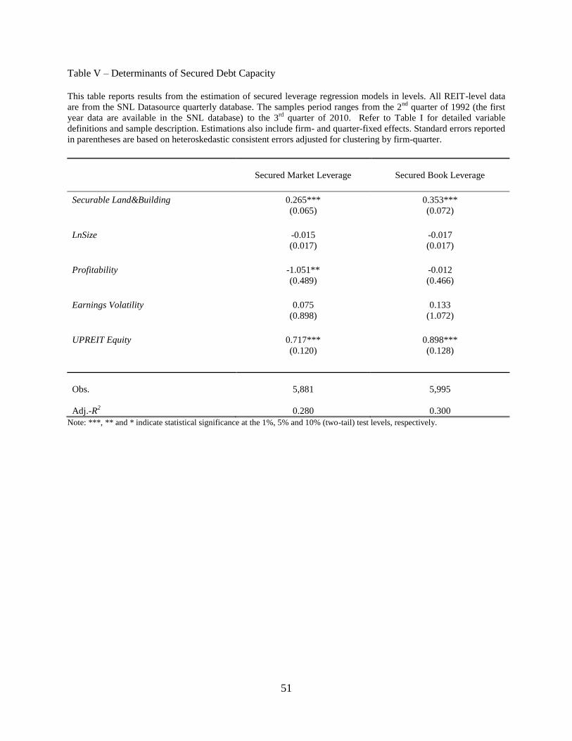
51

Table V – Determinants of Secured Debt Capacity This table reports results from the estimation of secured leverage regression models in levels. All REIT-level data

are from the SNL Datasource quarterly database. The samples period ranges from the 2nd

quarter of 1992 (the first

year data are available in the SNL database) to the 3rd

quarter of 2010. Refer to Table I for detailed variable

definitions and sample description. Estimations also include firm- and quarter-fixed effects. Standard errors reported

in parentheses are based on heteroskedastic consistent errors adjusted for clustering by firm-quarter.

Secured Market Leverage

Secured Book Leverage

Securable Land&Building 0.265*** 0.353***

(0.065) (0.072)

LnSize -0.015 -0.017

(0.017) (0.017)

Profitability -1.051** -0.012

(0.489) (0.466)

Earnings Volatility 0.075 0.133

(0.898) (1.072)

UPREIT Equity 0.717*** 0.898***

(0.120) (0.128)

Obs. 5,881 5,995

Adj.-R2 0.280 0.300

Note: ***, ** and * indicate statistical significance at the 1%, 5% and 10% (two-tail) test levels, respectively.

52

Table VI – ―Shocks‖ to the Secured Debt Market and q: Fannie-Freddie Financing for Housing REITs During the

Russian Crisis

This table reports results from the estimation of q regression models in changes. RussianCrisis is a dummy variable

that takes a value of 1 for the 3rd

and 4th

quarter of the year 1998 and zero otherwise. SecuredLeverageIncrease

(market and book) is a dummy variable that takes a value of 1 if the firm increases the use of its secured leverage

capacity in the current quarter relative to the prior quarter, where used secured leverage capacity is the difference

between observed secured leverage and secured debt capacity predicted from the estimation of secured debt

regressions reported in Table V. Housing REITs are listed-property firms with an investment focus on housing

properties (multi-family units) and access to Fannie-Freddie (backed) secured debt financing. Our regressor of

interest is the double-interaction term, which captures the difference-in-differences effect. All REIT-level data are

from the SNL Datasource quarterly database. The samples period ranges from the 2nd

quarter of 1992 (the first year

data are available in the SNL database) to the 3rd

quarter of 2010. Refer to Table I for detailed variable definitions

and sample description. Standard errors reported in parentheses are based on heteroskedastic consistent errors

adjusted for clustering at the firm-quarter level.

(1)

(2)

RussianCrisisSecuredMarketLeverageIncrease 0.035***

(0.006)

RussianCrisisSecuredBookLeverageIncrease 0.012***

(0.004)

RussianCrisis -0.044*** -0.032***

(0.005) (0.004)

SecuredMarketLeverageIncrease -0.026***

(0.006)

SecuredBookLeverageIncrease 0.006

(0.004)

UPREIT Equity -0.051 0.034

(0.082) (0.075)

LnSize -0.185*** -0.203***

(0.034) (0.034)

Profitability 0.034 -0.037

(0.600) (0.592)

EarningsVolatility 0.008 0.230

(1.234) (1.215)

Obs. 1,451 1,451

Adj.-R2 0.123 0.090

Note: ***, ** and * indicate statistical significance at the 1%, 5% and 10% (two-tail) test levels, respectively.

53

Table VII – ―Shocks‖ to the Secured Debt Market and q: Falsification Tests

This table reports results from the estimation of q regression models in changes. In the interest of space, we only report the

coefficient estimate on the double interaction term, which captures the difference-in-differences effect. See Table VI for

variable definitions. Housing REITs are listed-property firms with an investment focus on housing properties (multi-

family units) and access to Fannie-Freddie (backed) secured debt financing. Non-Housing REITs are listed-property firms

with an investment focus on office, retail, industrial, hotel property types. We report results for the Non-Housing sample

as a group and for each of the property-type sub-samples separately. For comparability, in the first row we also report the

coefficients on the double interaction term for the Housing sample from Table VI. All REIT-level data are from the SNL

Datasource quarterly database. The samples period ranges from the 2nd

quarter of 1992 (the first year data are available in

the SNL database) to the 3rd

quarter of 2010. Refer to Table I for detailed variable definitions and sample description.

Standard errors reported in parentheses are based on heteroskedastic consistent errors adjusted for clustering at the firm-

quarter level.

Increase Secured Market

Leverage

Increase Secured Book

Leverage

Obs.

Housing and Non-Housing Financing

During the Russian Crisis

Housing: RussianCrisisSecuredLeverageIncrease 0.035*** 0.012***

(0.006) (0.004) 1,451

Non-Housing: RussianCrisisSecuredLeverageIncrease -0.019 0.003

(0.015) (0.007) 4,164

Office: RussianCrisisSecuredLeverageIncrease -0.012 0.007

(0.009) (0.010) 1,546

Retail: RussianCrisisSecuredLeverageIncrease -0.019* -0.003

(0.010) (0.012) 1,380

Industrial: RussianCrisisSecuredLeverageIncrease 0.007 -0.015

(0.017) (0.013) 492

Hotel: RussianCrisisSecuredLeverageIncrease -0.038 -0.021

(0.024) (0.031) 746

Note: ***, ** and * indicate statistical significance at the 1%, 5% and 10% (two-tail) test levels, respectively.

54

Table VIII – ―Shocks‖ to the Secured Debt Market and q: Fannie-Freddie Financing During the Subprime Crisis

This table reports results from the estimation of q regression models in changes. SubprimeCrisis is a dummy variable that

takes a value of 1 for the 3rd

and 4th quarter of the year 2007 and zero otherwise. SecuredLeverageIncrease (market and

book) is a dummy variable that takes a value of 1 if the firm increases the use of its secured leverage capacity in the

current quarter relative to the prior quarter, where used secured leverage capacity is the difference between observed

secured leverage and secured debt capacity predicted from the estimation of secured debt regressions reported in Table V.

Housing REITs are listed-property firms with an investment focus on housing properties (multi-family units) and access to

Fannie-Freddie (backed) secured debt financing. Non-Housing REITs are listed-property firms with an investment focus

on office, retail, industrial, and hotel property types. Our regressor of interest is the double-interaction term, which

captures the difference-in-differences effect. All REIT-level data are from the SNL Datasource quarterly database. The

samples period ranges from the 2nd

quarter of 1992 (the first year data are available in the SNL database) to the 3rd

quarter

of 2010. Refer to Table I for detailed variable definitions and sample description. Standard errors reported in parentheses

are based on heteroskedastic consistent errors adjusted for clustering at the firm-quarter level.

Housing REITs

Non-Housing REITs

(1) (2) (3) (4)

SubprimeCrisisSecuredMarketLeverageIncrease 0.048*** -0.004

(0.017) (0.015)

SubprimeCrisisSecuredBookLeverageIncrease 0.069** 0.017

(0.031) (0.014)

SubprimeCrisis -0124*** -0.139*** -0.057** -0.060***

(0.035) (0.015) (0.026)

(0.025)

SecuredMarketLeverageIncrease -0.025*** -0.024***

(0.006) (0.005)

SecuredBookLeverageIncrease 0.006 -0.001

(0.004) (0.004)

UPREIT Equity -0.035 0.054 -0.201 -0.186

(0.083) (0.076) (0.150) (0.157)

LnSize -0.195*** -0.215*** -0.112*** -0.122***

(0.033) (0.033) (0.023) (0.024)

Profitability -0.071 -0.481 -0.303 -0.603

(0.586) (0.569) (0.420) (0.417)

EarningsVolatility 0.178 0.442 -0.214 -0.211

(1.215) (1.173) (0.433) (0.438)

Obs. 1,451 1,451 4,164 4,164

Adj.-R2 0.148 0.120 0.076 0.053

Note: ***, ** and * indicate statistical significance at the 1%, 5% and 10% (two-tail) test levels, respectively.

55

Table IX – q and Secured Leverage by Inside Equity Groups

This table reports mean comparison tests for Change in q, Change in SecuredMarketLeverage and Change in

SecuredBookLeverage by restricted shares groups. Change in q is the change in Tobin’s q from the previous year.

Change in SecuredMarketLeverage is the ratio of secured debt issuance in the current year to the market value of the

firm at the end of the previous year. Change in SecuredBookLeverage is defined similarly. The results are based on

a simple mean comparison test between the above and below median groups based on restricted equity, where

restricted equity is defined as the ratio of restricted shares awarded to the CEO in a given year to total assets.

―Above Median‖ firms are those with restricted shares above the industry segment median. ―Below Median‖ firms

are those with restricted equity below the industry segment median. Restricted shares data are hand-collected from

annual reports. All remaining firm level data are from SNL Datasource. Refer to Table I for detailed variable

definitions and sample description.

Restricted Shares Groups

Above Median

Below Median

Difference

Above – Below Median

Change in q 0.058 -0.001 0.057***

Change in SecuredMarketLeverage

0.031

0.069

-0.049***

Change in SecuredBookLeverage

0.040

0.078

-0.038***

Note: *** indicates statistical significance at the 1% (two-tail) test levels, respectively.

56

Figure 1 – BBB Housing REIT Bonds and Housing Mortgage Spreads During the Russian Crisis

This figure displays the spreads of BBB REIT bond yields and Freddie-Mac rates (Housing Mortgage) over the 10-

year and the 30-year Treasury bond yields respectively. The bond yield data is from Datastream. Freddie-Mac rates

are obtained from the webpage of the Federal Reserve Board.

0

50

100

150

200

250

Sp

read

s o

ver

Tre

asury

Bo

nd

Yie

lds

BBB REIT Bond Spread Housing Mortgage Spread

57

Figure 2 – Secured Debt Issuance, Unsecured Debt Issuance, and Investment for Housing REITs During the

Russian Crisis

This figure displays net secured debt issuance, net unsecured debt issuance, and investment as a percentage of total

assets for Housing REITs in the period surrounding the peak of the Russian crisis, which we identify as the 3rd

and

4th

quarters of 1998. The data is from the SNL Datasource quarterly database.

-1%

0%

1%

2%

3%

4%

5%

6%

1998Q1 1998Q2 1998Q3 1998Q4 1999Q1 1999Q2

Secured Debt Issuance Unsecured Debt Issuance Investment

58

Figure 3 – Line of Business Focus

This figure displays the average Herfindhal index (HHI) of business concentration for Housing and Non-Housing

REITs. The HHI index is based on the number of properties that firms have in each different property type,

including housing (multi-family units), office, retail, industrial, and hotel. For example, a Housing REIT with an

HHI index of 90% has 90% of its properties concentrated in the housing business. The data are from the SNL

Datasource annual database.

40%

50%

60%

70%

80%

90%

100%

1996 1997 1998 1999 2000

HHI Housing HHI Non-Housing