utilization of rain water harvesting and appropriately ... of rain water... · utilization of rain...
TRANSCRIPT
UNIVERSITÀ DEGLI STUDI DI FIRENZE
FIRST LEVEL MASTER DEGREE IN
IRRIGATION PROBLEMS IN DEVELOPING COUNTRIES
Thesis on:
UTILIZATION OF RAIN WATER HARVESTING AND
APPROPRIATELY DESIGNED DRIP IRRIGATION SYSTEMS TO
IMPROVE CROP PRODUCTION FOR SMALL HOLDER
FARMERS IN THE SEMI-ARID AREA OF MAAI-MAHIU IN
NAKURU COUNTY (KENYA).
By
PETER MBUGUA NJUGUNA
SUPERVISOR: DR. IVAN SOLINAS
A.A. 2013/2014

i
THESIS APPROVAL
Supervisor: Dr. Ivan Solinas
Supervisor’s signature: ...…………………..…….……………………………
Date:……...............................................................................................................
Student: Peter Mbugua Njuguna
Student’s signature:…………………………..…………..…...………..............
Date:…………..…………………………………..…...…………………………

ii
Dedication
To my beloved wife Jane, children Rose and Njuguna to their love and
dedication
iii
ACKNOWLEDGEMENT
Firstly, I am sincerely grateful to the Italian Ministry of Foreign Affairs, Italian
cooperation office in Nairobi, Instituto Agronomical per L‘Oltremare (IAO) and
the Universita Degli Studi Di Firenze for their financial support in the form of a
scholarship to undertake this first level master degree in irrigation problems in
developing countries.
I am grateful to the General Director of IAO, the Technical Director Dr. Tiberio
Chiari, the Coordinator of the irrigation Master Professor Eng. Elena Bresci, the
Administrative Assistant Dr Andrea Merli, the Academic Tutor, Dr Elisa Masi,
and all academic and non academic staff of IAO who supported me in various
ways during my studies here in Florence, Italy.
I would like to thank my supervisor, Dr. Ivan Solinas for the support, guidance and
constructive comments throughout this study. Without his tireless efforts and
commitment this study would not have been accomplished.
I would like to extend my heartfelt gratitude and love to my parents, my father
Njuguna Iraya, my late mother Loise Wanjira and all my brothers and sisters.
Their support and encouragement from my early childhood has given me the
energy and courage to overcome all the life hurdles.
In a special way, I would like to express my sincere gratitude and love to my
dear wife Jane Waitherero, for her care and affection in particular and for her love
and endurance at large. I would also like to thank her sincerely for being patient
when I was studying. Thank you for your prayers, love, support and
encouragement.
Special thanks also goes to my daughter Rose Wanjira and son Ezekiel Njuguna
.You have been strong and endured loneliness while dad was absent for 8 months.
Finally I would wish to thank my friends and colleagues in the 6th
and last
Edition of the First level Masters in Irrigation Problems in Developing
Countries. I would forever be grateful for the support and good time we had
together in Florence.

iv
PREFACE
Thesis report submitted for partial fulfillment for the award of the first level
master degree in irrigation problems in developing countries of Instituto
Agronomical per L‘Oltremare (IAO) and the Universita Degli Studi Di Firenze.
v
ABSTRACT
Smallholder farmers are the backbone of Kenya‘s agriculture and feed millions of
people with the fruits of their labour. They produce over 80 per cent of food for
the population and influence greatly the overall economical performance of the
country. In 2012 for example, Kenya‘s GDP stood at USD 43.18 billion with an
annual growth rate of 4.6 percent. Agriculture contributed 16.6 percent to the
GDP. Approximately 74 percent of the economically active population is
employed in agriculture.
ASAL areas cover approximately 80% of Kenya's land surface. In the recent past,
there has been a substantial increase in settlements within these areas that were
predominantly used for livestock production. In addition the ASAL areas are home
to more than 35% and 50% of human and livestock population respectively.
Rainfall in these areas is normally low, erratic and unreliable with frequent dry
spells even within the rainy seasons. This unreliability and poor distribution of
rainfall is the most limiting factor to agricultural production and human settlement.
Rainwater harvesting and drip irrigation are appropriate technologies that can
enhance agricultural production in Arid and Semi-Arid Lands (ASAL). Majority
of households living in these areas (ASALs) solely depend on agriculture for their
livelihoods. Moreover Kenya has over 80% of the arable land is located in water
scarce areas with recurrent dry spells.
It is evident from experiences in Kenya that rainwater harvesting could provide the
long sought answer to water scarcity. However, some technical hindrances need to
be addressed. Lack of appropriate technical designs, among other factors, has led
to low adoption of rainwater harvesting technology, especially in Arid and
Semiarid Lands (ASAL), where rainwater is one of the most viable sources of
cheap water.
RWH technologies to address rainfall variability are being developed and
promoted by public research and development institutions for these areas.
However, water harvesting technologies cannot be viewed in isolation. Its
introduction has to be integrated with appropriate techniques in this case efficient
drip irrigation. The main objective of this thesis is to model runoff harvesting and
design an efficient drip irrigation system for small holder farmers fed by gravity
based on the prevailing climatic conditions, soil and crop water requirements of
commonly grown crops in Maai-Mahiu area of Nakuru county in Kenya.
vi
The Crop water requirements have been determined with the software CROPWAT
8.0 based on local climatic data and field conditions. The on field water harvesting
investigation has been done through research and an elaborate explanation of how
to construct a dam has been provided. The runoff potential from rainfall water
harvesting has been done using Runoff curve number method. Drip irrigation has
been utilized in this study as it‗s the most efficient type of irrigation to save on the
much needed water resource. The irrigation design and network has been done
using the Ve.Pro.LG, and EPANET software for hydraulic modeling. Other
applications used include Google Earth, ClimWat, Harmonised World soil
Database (HWSD) and New LocClim.
vii
Table of Contents
THESIS APPROVAL ................................................................................................................. i
ACKNOWLEDGEMENT ..........................................................................................................iii
PREFACE ............................................................................................................................... iv
ABSTRACT............................................................................................................................. v
LIST OF FIGURES ....................................................................................................................x
LIST OF TABLES ..................................................................................................................... xi
LIST OF ABBREVIATIONS AND ACRONYMS ......................................................................... xii
1.0 INTRODUCTION .............................................................................................................. 1
1.1 Background Information ............................................................................................ 1
1.2 Problem Statement. ................................................................................................. 5
1.3 Objectives .............................................................................................................. 6
1.3.1 Main objective .................................................................................................... 6
1.3.2 Specific objectives ................................................................................................... 6
1.4 Justification. ............................................................................................................... 6
2.0 LITERATURE REVIEW ...................................................................................................... 9
2.1 What are Asal areas? ................................................................................................. 9
2.2 Rain Water Harvesting ............................................................................................... 9
2.2.1 Benefits of Rain Water Harvesting .................................................................... 10
2.2.2 Components of Water Harvesting Systems ...................................................... 10
2.2.3 Design of Water harvesting systems ................................................................ 11
2.2.4 Macro catchment and Floodwater Systems ..................................................... 11
2.2.5 Runoff Management. ........................................................................................ 12
2.2.6 Factors to consider when designing water storage facility. ............................. 12
2.2.7 Design and construction ................................................................................... 13
2.2.8 Water Storage Facilities .................................................................................... 13
2.3 Irrigation .................................................................................................................. 14
2.3.1 Drip Irrigation .................................................................................................... 15
2.3.2 Advantages of drip irrigation ............................................................................ 16
2.3.3 Problems associated with drip irrigation .......................................................... 17
viii
2.4 Choice of crops in this study .................................................................................... 18
2.4.1 Tomato Cultivation ........................................................................................... 19
2.4.2 Cultivation of Capsicum Pepper ........................................................................ 20
2.4.3 Cabbage Cultivation .......................................................................................... 22
2.5 Determination of Crop Water Requirements .......................................................... 23
2.6 Planting Dates .......................................................................................................... 28
3.0 MATERIAL AND METHODS ........................................................................................... 29
3.1 Description of the area of study .............................................................................. 29
3.1.1 Location and climatic conditions ...................................................................... 29
3.2 DESIGN SOFTWARE .................................................................................................. 32
3.2.1 Google earth ..................................................................................................... 32
3.2.2 Harmonised World soil Database (HWSD) ........................................................ 33
3.2.3 Soil water characteristics .................................................................................. 33
3.2.4 ClimWat ............................................................................................................ 34
3.2.5 New LocClim ..................................................................................................... 34
3.2.6 CropWat 8.0 ...................................................................................................... 34
3.2.7 Epanet ............................................................................................................... 35
3.2.8 Ve.pro.LG.s ........................................................................................................ 35
3.3 Source of water for irrigation. ............................................................................. 35
3.4 Estimating runoff using the runoff curve number method. ................................ 36
3.4.1 Design parameters ............................................................................................ 36
3.4.2 Curve Number Selection ................................................................................... 37
3.4.3 Run off Estimation in the Study Area ................................................................ 38
3.4.4 Design of Earth dam for RWH ........................................................................... 46
3.4.5 Reducing Dam Water Losses ............................................................................. 47
3.5 Design of irrigation Scheme ..................................................................................... 48
3.5.1 Crop Water Requirements of Each Crop........................................................... 48
3.5.2 Irrigation requirement: ..................................................................................... 49
3.5.3 Irrigation Scheduling: ........................................................................................ 49
3.5.4 Irrigation Scheme Supply .................................................................................. 50
ix
3.5.5 Cropping Pattern and Gross Irrigation Requirement ........................................ 51
4.0 RESULTS AND DISCUSSIONS ......................................................................................... 53
4.1 Drip irrigation system design ................................................................................... 53
4.1.1 Study Field Plot Geometry .............................................................................. 53
4.1.2 Design Scheme Water Requirement ................................................................. 54
4.2 Drip line Design using Ve.Pro.LG .............................................................................. 55
4.2.1 Ve.pro.LG.s. Results and discussion .................................................................. 55
4.3 Pipe Line Design using EPANET ................................................................................ 56
4.4 Discussion ................................................................................................................ 61
4.4.1 Discussion of RWH Potential results. ................................................................ 61
4.4.2 Discussion of irrigation system design results: ................................................. 61
5.0 CONCLUSION AND RECOMMENDATIONS.................................................................... 63
5.1 Conclusion ................................................................................................................ 63
5.2 Recommendations ................................................................................................... 64
REFERENCES ....................................................................................................................... 66
APPENDIX ........................................................................................................................... 68
x
LIST OF FIGURES
Figure 1:Manual construction of RWH structures in Yatta, Kenya. The ponds are
used to grow high value crops.(Courtesy MOA) ................................................... 14
Figure 2: Drip Irrigation in dry lands. .................................................................... 18
Figure 3: Crop Co-efficient (Kc) at different growth stage .................................... 27
Figure 4: Location of Maai-Mahiu Division, Nakuru in Kenya ............................. 30
Figure 5: Comparison of ETo and Effective Rain in Maai-Mahiu. ........................ 31
Figure 6: Maai-Mahiu Soil Water Characteristics ................................................. 34
Figure 7: New-LocClim extract illustration of seasons. ......................................... 39
Figure 8.Extract from Google maps showing the estimated catchment area of the
study area. ............................................................................................................... 42
Figure 9: Extract of Excel file used for the calculation of runoff. ......................... 43
Figure 10: Average annual monthly runoff (mm). ................................................. 46
Figure 11: Field Layout as taken on Google earth. ................................................ 54
Figure 12 : Network of design. ............................................................................... 59
Figure 13: Distribution system network to the plots. ............................................. 60
Appendix A 1: CROPWAT 8.0 working Analysis ................................................ 68
Appendix A 2: Ve.Pro.LG Analysis ...................................................................... 73
Appendix A 3: Epanet Analysis ............................................................................. 75
Appendix A 4: Run off estimation ......................................................................... 78
xi
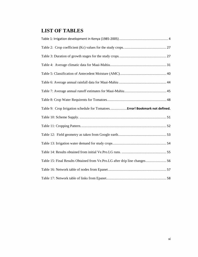
LIST OF TABLES
Table 1: Irrigation development in Kenya (1985-2005) ....................................................... 4
Table 2: Crop coefficient (Kc) values for the study crops. ............................................... 27
Table 3: Duration of growth stages for the study crops. .................................................... 27
Table 4: Average climatic data for Maai-Mahiu. .............................................................. 31
Table 5: Classification of Antecedent Moisture (AMC). ................................................... 40
Table 6: Average annual rainfall data for Maai-Mahiu ..................................................... 44
Table 7: Average annual runoff estimates for Maai-Mahiu ............................................... 45
Table 8: Crop Water Requirents for Tomatoes .................................................................. 48
Table 9: Crop Irrigation schedule for Tomatoes. .................. Error! Bookmark not defined.
Table 10: Scheme Supply. ................................................................................................. 51
Table 11: Cropping Pattern. ............................................................................................... 52
Table 12: Field geometry as taken from Google earth...................................................... 53
Table 13: Irrigation water demand for study crops ............................................................ 54
Table 14: Results obtained from initial Ve.Pro.LG runs. .................................................. 55
Table 15: Final Results Obtained from Ve.Pro.LG after drip line changes ....................... 56
Table 16: Network table of nodes from Epanet ................................................................. 57
Table 17: Network table of links from Epanet ................................................................... 58
xii
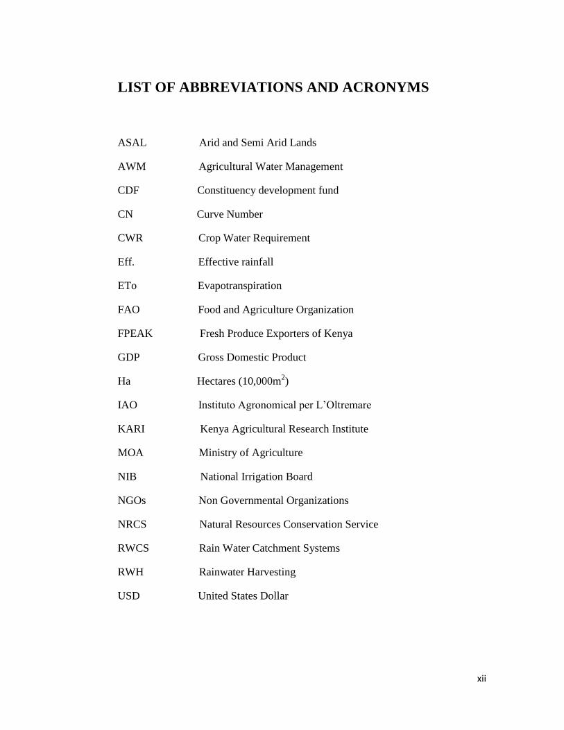
LIST OF ABBREVIATIONS AND ACRONYMS
ASAL Arid and Semi Arid Lands
AWM Agricultural Water Management
CDF Constituency development fund
CN Curve Number
CWR Crop Water Requirement
Eff. Effective rainfall
ETo Evapotranspiration
FAO Food and Agriculture Organization
FPEAK Fresh Produce Exporters of Kenya
GDP Gross Domestic Product
Ha Hectares (10,000m2)
IAO Instituto Agronomical per L‘Oltremare
KARI Kenya Agricultural Research Institute
MOA Ministry of Agriculture
NIB National Irrigation Board
NGOs Non Governmental Organizations
NRCS Natural Resources Conservation Service
RWCS Rain Water Catchment Systems
RWH Rainwater Harvesting
USD United States Dollar

1
1.0 INTRODUCTION
1.1 Background Information
Kenya is situated on the East African coast on the equator. It is bordered by
Ethiopia and South Sudan to the north, the Indian Ocean and Somalia to the east,
the United Republic of Tanzania to the south, and Uganda and Lake Victoria to the
west. The total area of the country is 582,646km2. Administratively the country is
subdivided into 47 semi autonomous counties and further into 290 sub-counties.
The altitude varies from sea level to the peak of Mt. Kenya, situated north of the
capital Nairobi, which is 5 199 meters above sea level.
The soil types in the country vary from place to place due to topography, the
amount of rainfall and the parent material. The soils in western parts of the country
are mainly acrisols, cambisols and their mixtures, highly weathered and leached
with accumulations of iron and aluminium oxides. The soils in central Kenya and
the highlands are mainly the nitosols and andosols, which are young and of
volcanic origin. The soils in the arid and semi-arid lands (ASAL) include the
vertisols, gleysols and phaeozems and are characterized with pockets of sodicity
and salinity, low fertility and vulnerability to erosion. Coastal soils are coarse
textured and low in organic matter and the common types are the arenosols,
luvisols and acrisols. Widespread soil salinity, which has adversely influenced
irrigation development, is found in isolated pockets around the Lake Baringo basin
in the Rift Valley and in the Taveta in the coastal provinces.
The average annual rainfall is 630 mm with a variation from less than 200 mm in
northern Kenya to over 1 800 mm on the slopes of Mt. Kenya. The rainfall
distribution pattern is bimodal with long rains falling from March to June and
short rains from October to November for most parts of the country. The climate is
influenced by the inter-tropical convergence zone and relief and ranges from
permanent snow above 4 600 meters on Mt. Kenya to true desert type in the Chalbi
desert in the Marsabit district in the north of the country. About 80 percent of the
country is arid and semi-arid, while 17 percent is considered to be high potential
agricultural land, sustaining 65 percent of the population. The forest cover is about
7 percent of the total land area.
Using Penman method annual evaporation from open water surfaces in Kenya is
estimated at a low of 1 000 mm in the central highlands to a high of 2 600 mm in
2
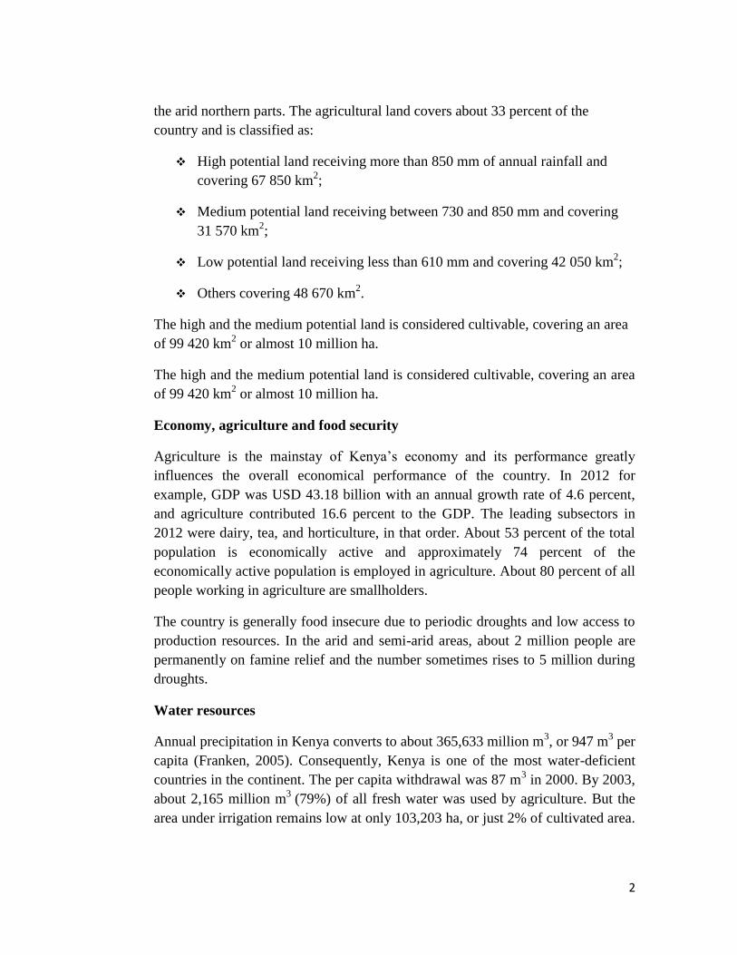
the arid northern parts. The agricultural land covers about 33 percent of the
country and is classified as:
High potential land receiving more than 850 mm of annual rainfall and
covering 67 850 km2;
Medium potential land receiving between 730 and 850 mm and covering
31 570 km2;
Low potential land receiving less than 610 mm and covering 42 050 km2;
Others covering 48 670 km2.
The high and the medium potential land is considered cultivable, covering an area
of 99 420 km2 or almost 10 million ha.
The high and the medium potential land is considered cultivable, covering an area
of 99 420 km2 or almost 10 million ha.
Economy, agriculture and food security
Agriculture is the mainstay of Kenya‘s economy and its performance greatly
influences the overall economical performance of the country. In 2012 for
example, GDP was USD 43.18 billion with an annual growth rate of 4.6 percent,
and agriculture contributed 16.6 percent to the GDP. The leading subsectors in
2012 were dairy, tea, and horticulture, in that order. About 53 percent of the total
population is economically active and approximately 74 percent of the
economically active population is employed in agriculture. About 80 percent of all
people working in agriculture are smallholders.
The country is generally food insecure due to periodic droughts and low access to
production resources. In the arid and semi-arid areas, about 2 million people are
permanently on famine relief and the number sometimes rises to 5 million during
droughts.
Water resources
Annual precipitation in Kenya converts to about 365,633 million m3, or 947 m
3 per
capita (Franken, 2005). Consequently, Kenya is one of the most water-deficient
countries in the continent. The per capita withdrawal was 87 m3 in 2000. By 2003,
about 2,165 million m3
(79%) of all fresh water was used by agriculture. But the
area under irrigation remains low at only 103,203 ha, or just 2% of cultivated area.
3
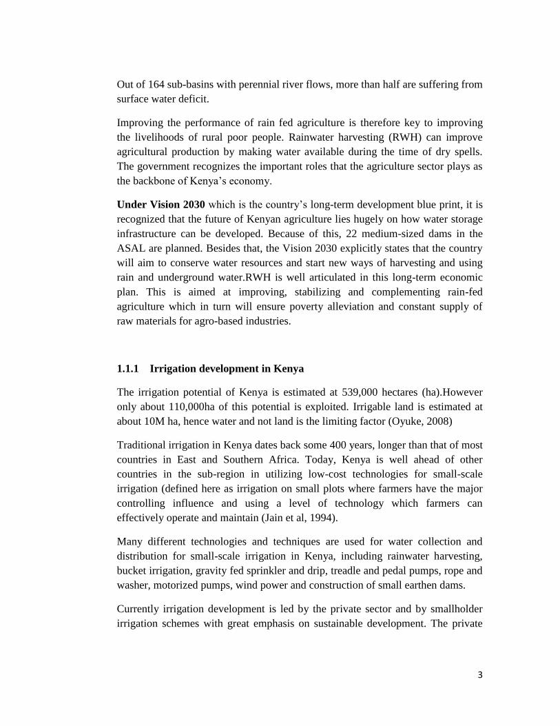
Out of 164 sub-basins with perennial river flows, more than half are suffering from
surface water deficit.
Improving the performance of rain fed agriculture is therefore key to improving
the livelihoods of rural poor people. Rainwater harvesting (RWH) can improve
agricultural production by making water available during the time of dry spells.
The government recognizes the important roles that the agriculture sector plays as
the backbone of Kenya‘s economy.
Under Vision 2030 which is the country‘s long-term development blue print, it is
recognized that the future of Kenyan agriculture lies hugely on how water storage
infrastructure can be developed. Because of this, 22 medium-sized dams in the
ASAL are planned. Besides that, the Vision 2030 explicitly states that the country
will aim to conserve water resources and start new ways of harvesting and using
rain and underground water.RWH is well articulated in this long-term economic
plan. This is aimed at improving, stabilizing and complementing rain-fed
agriculture which in turn will ensure poverty alleviation and constant supply of
raw materials for agro-based industries.
1.1.1 Irrigation development in Kenya
The irrigation potential of Kenya is estimated at 539,000 hectares (ha).However
only about 110,000ha of this potential is exploited. Irrigable land is estimated at
about 10M ha, hence water and not land is the limiting factor (Oyuke, 2008)
Traditional irrigation in Kenya dates back some 400 years, longer than that of most
countries in East and Southern Africa. Today, Kenya is well ahead of other
countries in the sub-region in utilizing low-cost technologies for small-scale
irrigation (defined here as irrigation on small plots where farmers have the major
controlling influence and using a level of technology which farmers can
effectively operate and maintain (Jain et al, 1994).
Many different technologies and techniques are used for water collection and
distribution for small-scale irrigation in Kenya, including rainwater harvesting,
bucket irrigation, gravity fed sprinkler and drip, treadle and pedal pumps, rope and
washer, motorized pumps, wind power and construction of small earthen dams.
Currently irrigation development is led by the private sector and by smallholder
irrigation schemes with great emphasis on sustainable development. The private
4
sector has also spearheaded irrigation development in areas close to urban centers
for local vegetables and high value horticultural produce for the export market.
The funding of irrigation development has shifted from government-led
development to participatory and community-driven development. As a result of
the change of approach and policy, irrigation development has been categorized so
that schemes in the arid and semi-arid lands (ASAL) have to be developed through
grants, with the beneficiaries providing contribution in terms of unskilled labour
and local materials. Community-based market-oriented irrigation schemes are
currently developed through cost-sharing rather than full cost recovery on
infrastructure. Full cost recovery approach has been discontinued because it has
been found to be a hindrance to irrigation development especially where major
infrastructure is involved. In both cases operation and maintenance are the
responsibility of the community.
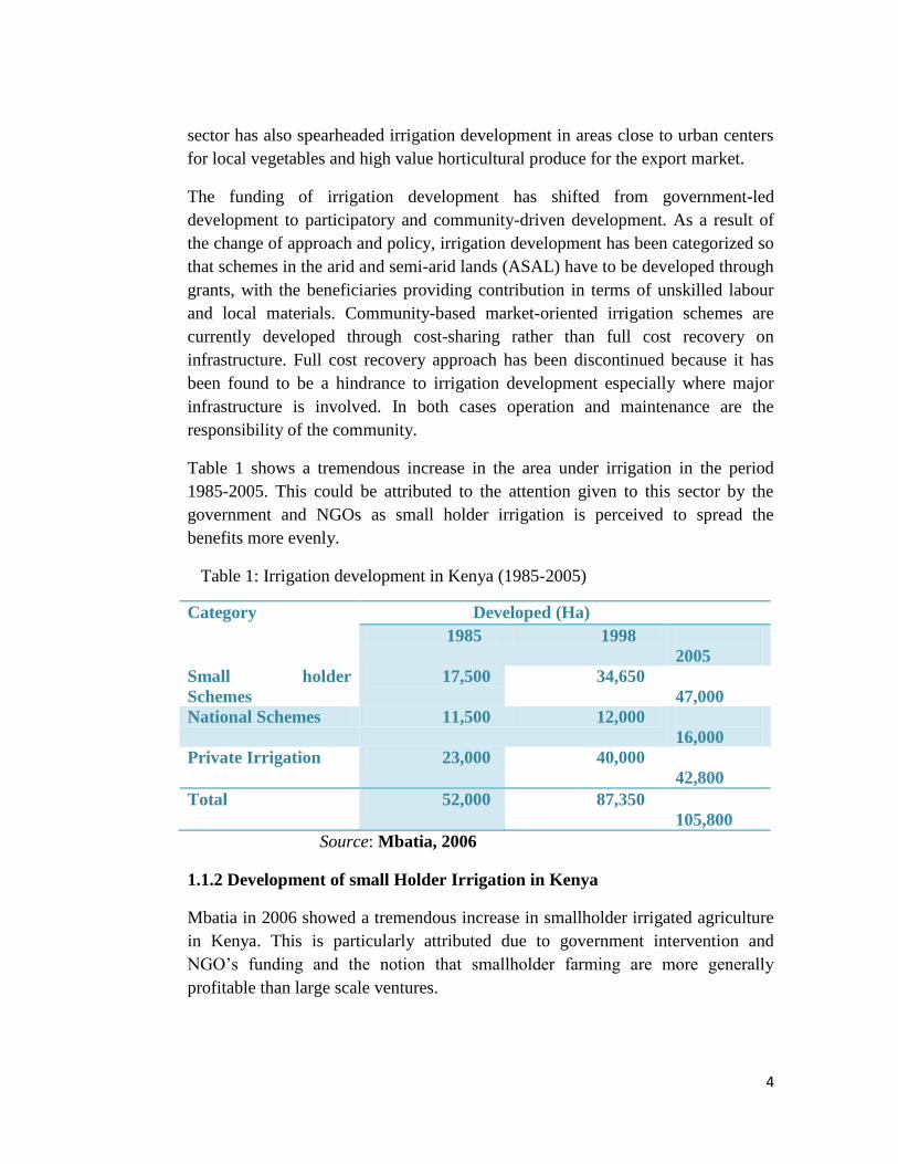
Table 1 shows a tremendous increase in the area under irrigation in the period
1985-2005. This could be attributed to the attention given to this sector by the
government and NGOs as small holder irrigation is perceived to spread the
benefits more evenly.
Table 1: Irrigation development in Kenya (1985-2005)
Category Developed (Ha)
1985 1998
2005
Small holder
Schemes
17,500 34,650
47,000
National Schemes 11,500 12,000
16,000
Private Irrigation 23,000 40,000
42,800
Total 52,000 87,350
105,800
Source: Mbatia, 2006
1.1.2 Development of small Holder Irrigation in Kenya
Mbatia in 2006 showed a tremendous increase in smallholder irrigated agriculture
in Kenya. This is particularly attributed due to government intervention and
NGO‘s funding and the notion that smallholder farming are more generally
profitable than large scale ventures.
5
1.2 Problem Statement.
Smallholder crop production is the backbone of Kenya‘s agriculture and is mainly
practiced under rain fed conditions. They produce over 80 per cent of food for the
population and influence greatly the overall economical performance of the
country. Approximately 74 percent of the economically active population is
employed in agriculture. A part of this crop production is done in semi-arid areas
such as Maai-Mahiu division.
Past studies have shown that agriculture in the ASALs of East Africa is mostly
rain-fed (Hatibu and Mahoo, 2000; Critchley, et al. 1999). Therefore, moisture
stress is a major constraint against food production in these areas. Demand for
water use in agriculture will continue to increase as a result of growing population
and economic growth (Rose grant, 2009).This poses a major threat to food
security. To guarantee food security, proper management of water resources is
absolutely necessary. This encompasses taking all deliberate human actions
designed to optimize the availability and utilization of water for agricultural
purposes (Mati, 2007).This includes practices such as irrigation (supplemental or
full), drainage, soil and water conservation, rainwater harvesting, soil fertility
management, conservation agriculture and wastewater reuse among others.
Water harvesting, is one of the techniques for supporting rain-fed agriculture in
the ASAL (Hai,1998;).Despite various non-governmental organizations and
government advocating the use of RWH to improve the livelihoods of rural
people, the implementation has been constrained by a number of challenges
leading to low adoption .Some RWH structures are not performing as anticipated
in terms of harvesting and storing adequate amounts of runoff to meet the water
demands particularly for crop production due to various reasons.
The main reason for this is inadequate information for proper planning of RWH
interventions. Currently, most RWH interventions are done on ad-hoc basis
without much knowledge about the location-specific conditions. A more
systematic approach to the selection of feasible sites for RWH interventions may
improve their performance and rate of adoption. For instance FAO (2003) as cited
by Kahinda et al. (2008) lists six key factors to be considered when identifying
RWH sites: climate (rainfall), hydrology (rainfall–runoff relationship and
intermittent water courses), topography (slope), agronomy (crop characteristics),
soils (texture, structure and depth) and socioeconomic criteria (population density,
work force, people‘s priority, experience with RWH, land tenure, water laws,
accessibility and related costs).
6
1.3 Objectives
1.3.1 Main objective
The main objective of this thesis is to model runoff harvesting and design an
efficient drip irrigation system for small holder farmers fed by gravity based on the
prevailing climatic conditions, soil and crop water requirements of major crops
grown in Maai-Mahiu area of Nakuru county in Kenya.
1.3.2 Specific objectives
To increase water productivity and reduce over reliance on rain fed
agriculture by leveraging on water harvesting and well designed and
efficient Irrigation systems;
To assess the potential of harvesting rainwater for crop production in
Maai-Mahiu by optimization of design parameters such as analysis of
rainfall, water demand, catchment area and storage capacity.
To assess the feasibility of gravity fed supplemental drip irrigation using
rainwater harvesting in the area.
To design and recommend the appropriate drip irrigation system for the
small holder farmers with reduced economic costs and high suitability for
the area.
1.4 Justification.
In the recent past, there has been a substantial increase in settlements within ASAL
areas, which covers over approximately 80% of Kenya's land surface. These areas
were predominantly used for livestock production. In addition the ASAL areas are
home to more than 35% and 50% of human and livestock population respectively.
Rainfall in these areas is normally low, erratic and unreliable rainfall, with
frequent dry spells even within the rainy seasons. This unreliability and poor
distribution of rainfall is the most limiting factor to agricultural production and
human settlement.
7
The problems posed by inadequate water supply are aggravated by population
growth, environmental degradation, and competition over the use of limited
natural resources and increasing water demand. There is need to develop
immediate, practical and sustainable solutions to address the twin problems of
inadequate water and food insecurity (Ngigi, 1999).
In Kenya, irrigation uses over 69 percent of the limited developed water resources
(Maff, 1976) and despite this high water use, the performance of irrigation projects
has not been impressive. Available water resources are diminishing, leading to
conflicts over water use among water users. The increasing demand for water for
the domestic and industrial sectors is expected to continue. This means that the
water use by the agriculture sector must be decreased to 33 percent by the year
2025 (Maff, 1976). This calls for more efficient use of water in irrigation. The
irrigation efficiency, which was estimated at 27 percent in 1990, should increase to
54 percent to reduce the water withdrawals in irrigation by the year 2025 (Maff,
1976).
One of the greatest possibilities for improving agriculture productivity in dry areas
is use of supplemental irrigation. This is a technology for providing additional
water to essentially rain-fed crops when rainfall is inadequate for normal plant
growth. The amount and timing of supplemental irrigation are scheduled aimed at
ensuring that there is a minimum amount of water available during critical stages
of crop growth for optimal crop yield. Harvested water is collected in a storage
structure and can be used later for supplemental irrigation.
In the recent past there has been a commendable increase in small holder irrigation
farming in Kenya with far better results than large scale irrigation schemes.
However Smallholder drip irrigation systems are faced with numerous challenges
some of which are technical in nature, economic constraints and resulting to
environmental degradations. This is mainly due to disregard to basic principles of
water resource conservation and sustainability. (Of which little studies have been
undertaken).
Inappropriate skills in irrigation system selection, design and management is a
common phenomena in most smallholder systems in Kenya as shown by Kay et al
(1992).Ensuing environmental degradation is also very common. Low water use
efficiency, soil salinity, insect pest damage, plant diseases and poor crop
husbandry negatively influence crop production under irrigated farming, (Sijali,
2000). He further noted that smallholder farmers tend to look for irrigation
technologies they can understand and afford to buy.

8
High investment costs also limit development of smallholder drip irrigation
systems in Kenya, (Gay, 1994).
It is clear now more than ever before that unless concerted efforts are made to
reduce the crippling uncertainty of rain-fed agriculture through RWH and
irrigation, many farmers will fight a losing battle with a hostile climate.
9
2.0 LITERATURE REVIEW
2.1 What are Asal areas?
Arid and semi-arid Lands (ASAL) are those characterized by low erratic rainfall of
up to 750mm per annum, periodic droughts and different associations of vegetative
cover and soils. Inter annual rainfall varies from 50-100% in the arid zones of the
world with averages of up to 350 mm. In the semi-arid zones, inter annual rainfall
varies from 20-50% with averages of up to 700 mm. Regarding livelihoods
systems, in general, light pastoral use is possible in arid areas and rain fed
agriculture is usually not possible. In the semi-arid areas agricultural harvests are
likely to be irregular, although grazing is satisfactory (Goodin & Northington,
1985).
The ASAL in Kenya covers over 80 % of the country. These vast lands are
generally poor and experience food scarcity. Accurate knowledge of soil water
content, in ASAL areas is essential for proper soil water management, irrigation
scheduling and crop production. However, the data necessary for sound
agricultural water management is often scarce.
2.2 Rain Water Harvesting
There are variations in definition depending on the source of information.
However, rainwater harvesting can be defined as those methods of collection,
concentration and storage of various forms of runoff from a variety of sources for
later use.
Water Harvesting is an ancient technology used in dry areas of the world.
Literature indicates that it has been around for several thousand years around the
Middle East. Current use can be observed in Africa, Asia, Australia, the Americas
and the Middle East.
Water harvesting can looked at as an intermediate level technology. Where rainfall
is low or poorly distributed it may be too unreliable for cropping. The alternative
to this scenario is irrigation. However, this may not be practiced, as water is not
adequate or available at all. Water harvesting therefore provides a middle-level
solution to agriculture in dry areas. When irrigation water becomes available,
farmers can upgrade to full scale irrigation.
10
The technology finds ready use for domestic, livestock and crop water. It is an
important technology for remote areas and areas with medium to low rainfall.
Runoff can be harvested near the point of use or at a location remote to the source.
Classification of water harvesting systems is based on this criterion. Water storage
is an important part of any water harvesting system. Its principal use is to help
people cope with poor rainfall distribution and avail required water long after rains
have ceased. Storage is cheapest when done in the root zone. However, this may
not always be adequate or practical, and other forms of storage infrastructure may
be necessary.
2.2.1 Benefits of Rain Water Harvesting
Water harvesting offers considerable scope for increasing agricultural productivity
in arid and semi-arid areas. It complements existing water or soil moisture
conservation systems. Besides crops, harvested water can be used for domestic
needs, livestock use, erosion reduction and crops establishment. The latter is
particularly important as semi-arid areas have a wider crop adaptation if water
shortages can be alleviated.
A study done in Mwala division in Eastern Kenya on the impact of run-off water
harvesting for dry spell mitigation in maize showed that harvesting runoff water
for supplemental irrigation is a risk-averting strategy, pre-empting situations where
crops depend on rainfall that is highly variable both in distribution and amounts
(Barron and Okwach 2005). Water harvested and stored in an earthen dam
provided a technically feasible option to supplement crop water demand.
2.2.2 Components of Water Harvesting Systems
Any water harvesting system consists of three basic components:
Catchment area
The area of a catchment is the most important property of the catchment. The
potential runoff volume is determined by the size of the catchment, provided the
storm covers the whole area. It is the part of land that contributes some of the
rainwater to a target area outside its boundaries. It can be as small a few square
meters or several square kilometers. Catchment surfaces are either natural or
modified.
11
Water Storage Reservoir
This is a designated space for storage of runoff water once it is harvested. Storage
can be in surface reservoirs, subsurface reservoirs, the soil profile, and ground
water aquifers.
Water Use area
In respect of agricultural production (including trees), this is where harvested
water is applied. This is defined differently for domestic or livestock use.
2.2.3 Design of Water harvesting systems
All water harvesting systems are designed to meet an objective. The principal
objective is to meet water requirements of the system. If the system is designed for
a crop, the objective would be to supply water to the growing crop and as and
when it is needed.
A water harvesting system consists of a catchment area and a crop area. The crop
area is determined by the farmer for row crops and by the tree canopy for single
trees. In practice, a crop area will be made up of many such areas; for trees, the
canopy area approximately defines a crop area, and a design is based on the
canopy of a mature tree. The basic formula used in water harvesting determines
the catchment to crop area ratio:
Where
IR=Irrigation requirement for the crop in question (mm); R=design rainfall (mm);
C=runoff coefficient (fraction, E=efficiency factor.
2.2.4 Macro catchment and Floodwater Systems
Macro catchment and floodwater harvesting systems are characterized by runoff
water collected from relatively large catchment areas. The catchment is a natural
rangeland, hill slope or a mountainous area. Catchments for these systems are
mostly located outside farm boundaries, where individual farmers have little or no
control over them. The macro catchment system consists of upland runoff
12
harvesting and farming before water reaches natural drainage channels. For these
systems the CCAR may be 10:1 to 100:1.
Generally, runoff capture is much lower than for micro catchments. Runoff water
is often stored in soil profile for direct use by crops, but may also be stored in
surface or subsurface reservoirs for later use. The cropped area is either terraced
on gentle slopes or located on flat terrain.
2.2.5 Runoff Management.
Water harvesting technologies enable more reliable plant production. However it
has certain drawbacks that need to be acknowledged. There is need to recognize
that water harvesting is not effective in all situations or in all years. In years of
very limited rainfall, water harvesting will simply not work. In years of excessive
rainfall water harvesting can produce negative results since drainage, not
harvesting, would be more desirable. It can result in loss of land where a specific
area is principally used as a catchment rather than for cropping, and the overall
production could be smaller even if more reliable.
2.2.6 Factors to consider when designing water storage facility.
While undertaking any RWH activity, it is important to put the following factors
into consideration;
Capacity of storage
The storage capacity depends on available runoff and intended use and time length
of use. Any storage structure is therefore made to significantly meet needs for a
specified time.
Location of storage
This depends on topography, method of water withdrawal and the source of runoff
water to be harvested.
Type of storage
This depends on the type of construction material, surface or underground
reservoir, dam or pond, and whether the structure is in-stream or off-stream.
Geometry
13
There is need to maximize the ratio of volume of storage volume (S) to the volume
of earth (E) that is excavation (S/E). Designs also aim to minimize surface area for
any given storage volume in order to reduce surface losses through evaporation.
The selection of the shape free: it can be rectangular, square, cylinder,
hemispherical or spherical.
Diversion, Conveyance and Spillway
These are required for almost all RWH systems. They principally serve two
purposes: 1) safety and 2) adequate capacity. There should be no sliding or tipping
over of diversion weir and no erosion or overtopping of conveyance channel and
the spillway. The design of these components is given in a variety of text books
and manuals (e.g. Thomas, 1997).
2.2.7 Design and construction
Designers should consult engineering handbooks for general specification,
conditions and technical requirements. Dams require that beyond a certain dam,
size only registered engineers design them. This is to avoid errors and possible
failure and loss of human life and property downstream. However design of off-
stream ponds is much more flexible and more people with basic knowledge can
design and implement them.
2.2.8 Water Storage Facilities
Earth Dams
Earth dams can be designed to store from 500-10,000 cubic meters. The dam wall
can be 5 meters high (dams over 15m would can only be designed by a qualified
engineer). Dams can be built by using manual labour and animal traction using ox-
scoops. Larger ones can be made using heavy machinery where available. Dams
can start small and then they are extended over time. Dams are usually made on
streams that experience runoff flow when it rains.
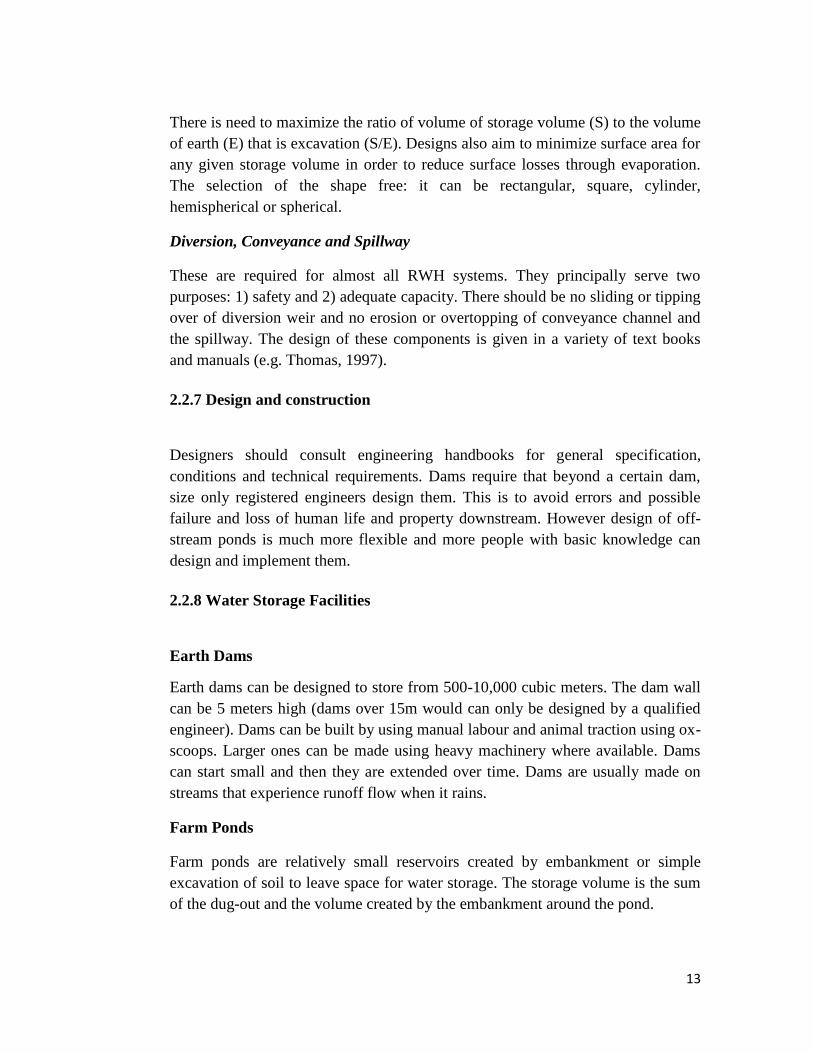
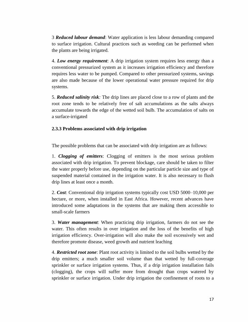
Farm Ponds
Farm ponds are relatively small reservoirs created by embankment or simple
excavation of soil to leave space for water storage. The storage volume is the sum
of the dug-out and the volume created by the embankment around the pond.
14
The objective of a farm pond is to capture and store runoff from rainfall and later
make it available for agricultural production. Depending on prevailing
circumstances, such ponds can also be used to integrate fisheries, and this
enhances food security and resource productivity. This technique is suitable to
nearly all land uses. However, it requires reasonably level topography and where
soils have low seepage rates. They are most suitable in drier climates where
rainfall reliability is a problem for agriculture.
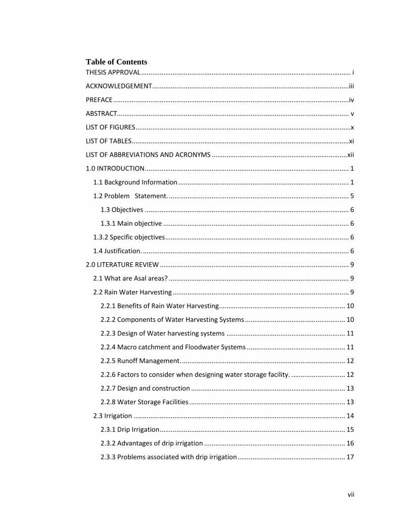
Figure 1:Manual construction of RWH structures in Yatta, Kenya. The ponds are used to grow high value crops.(Courtesy MOA)
2.3 Irrigation
Irrigation is the act of delivering and applying water necessary for plant life,
growth and environmental care. The technology used has to be appropriate for it to
be adopted by irrigators.
15
Main irrigation methods in Kenya include; Hand watering, flood irrigation,
overhead sprinkler, surface drip irrigation and Subsurface drip irrigation. The
choice of technology used mainly depends on soil, water availability, climate,
slope and water quality among other factors
Aims of Irrigation
In summary irrigation is basically aimed at:
Maintaining soil water moisture to achieve optimal yield
Stabilising crop productivity against droughts and in-season dry spells
Increasing crop yields per unit area through relay cropping
Providing water during the dry season to facilitate crop diversification
Improving people‘s welfare through improved crop yields and incomes
Leaching excess soil salts from the root zone
In some cases, chemicals like fertilisers (fertigation) are mixed with
irrigation water and directly applied to the crops.
2.3.1 Drip Irrigation
The drip irrigation (also called micro sprinkler irrigation) methods provide good
water control by delivering water in the plant root zone; enabling the farmer to
grow crops with much less water compared to other irrigation methods. It is
defined as the slow application of water to the soil surface as discrete or
continuous drops. Water is applied to the soil through emitters at operating
pressures of 0.5-2.0 bar and a discharge rate of about 1-16 l/h. It allows increasing
water use efficiencies by providing precise amounts of water directly to the root
zone of individual plants (Burt and styles 2007).
The first drip irrigation experiments are reported to have began in Germany in
1860.In the united states, they started around 1873.Experiments with perforated
pipes were introduced in 1920,providing an important breakthrough and leading to
the development of entire irrigation systems using perforated pipes made of
various materials.
16
It consists of an extensive network of pipes, usually of small diameters, that
deliver water directly to the soil near the plant. It allows increasing water use
efficiencies by providing precise amounts of water directly to the root zone of
individual plants (Burt and Styles, 2007). A dripline system consists of pipe
system fixed with emitters, laterals, manifold and mainline, which transport water
from the source to plant root zone. The mainline delivers water to manifold and
manifold delivers water to laterals. Each plant is provided with a continuous
readily available supply of water to meet transpiration demands (Keller and
Karmeli, 1974). Water filtration is provided for to remove suspended materials,
organic matter, sand and clay to reduce blockage of the emitters. To maintain
required pressure heads control valves must be included.
Drip irrigation systems can be categorised into two; Surface and Sub-surface.
Surface drip irrigation system is whereby the drip tape is on the surface, (i.e.) the
point of water application is on the surface. Sub-surface drip irrigation is whereby
the drip tape is buried and water application is by underground wetting. (Ngigi,
2010).
In the last 15 years, drip irrigation systems that operate under pressure lower than
0.5 bars have been promoted among the smallholder farmers in Kenya. Operating
the drip irrigation systems under pressure in the range of 0.05 to 0.5bar is referred
to as low head.
The basic components of a drip system include; Emitters, Water delivery and
distribution pipes, Filter, Control unit and Raised reservoir or pump.
2.3.2 Advantages of drip irrigation
1 More efficient use of water: Compared to surface irrigation and sprinkler
methods (with efficiencies of 50–75% in high-management systems), drip
irrigation can achieve 90–95% efficiency. This is because percolation losses are
minimal and direct evaporation from the soil surface and water uptake by weeds
are reduced by not wetting the entire soil surface between plants .
2 Reduced cost for fertilizers: Precise application of nutrients is possible using
drip irrigation. Fertilizer costs and nitrate losses can be reduced considerably when
the fertilizers are applied through the irrigation water (termed fertigation). Nutrient
applications can be better timed to coincide with plant needs since dressing can be
carried out frequently in small amounts and fertilizers are brought to the
immediate vicinity of the active roots.
17
3 Reduced labour demand: Water application is less labour demanding compared
to surface irrigation. Cultural practices such as weeding can be performed when
the plants are being irrigated.
4. Low energy requirement: A drip irrigation system requires less energy than a
conventional pressurized system as it increases irrigation efficiency and therefore
requires less water to be pumped. Compared to other pressurized systems, savings
are also made because of the lower operational water pressure required for drip
systems.
5. Reduced salinity risk: The drip lines are placed close to a row of plants and the
root zone tends to be relatively free of salt accumulations as the salts always
accumulate towards the edge of the wetted soil bulb. The accumulation of salts on
a surface-irrigated
2.3.3 Problems associated with drip irrigation
The possible problems that can be associated with drip irrigation are as follows:
1. Clogging of emitters: Clogging of emitters is the most serious problem
associated with drip irrigation. To prevent blockage, care should be taken to filter
the water properly before use, depending on the particular particle size and type of
suspended material contained in the irrigation water. It is also necessary to flush
drip lines at least once a month.
2. Cost: Conventional drip irrigation systems typically cost USD 5000–10,000 per
hectare, or more, when installed in East Africa. However, recent advances have
introduced some adaptations in the systems that are making them accessible to
small-scale farmers
3. Water management: When practicing drip irrigation, farmers do not see the
water. This often results in over irrigation and the loss of the benefits of high
irrigation efficiency. Over-irrigation will also make the soil excessively wet and
therefore promote disease, weed growth and nutrient leaching
4. Restricted root zone: Plant root activity is limited to the soil bulbs wetted by the
drip emitters; a much smaller soil volume than that wetted by full-coverage
sprinkler or surface irrigation systems. Thus, if a drip irrigation installation fails
(clogging), the crops will suffer more from drought than crops watered by
sprinkler or surface irrigation. Under drip irrigation the confinement of roots to a
18
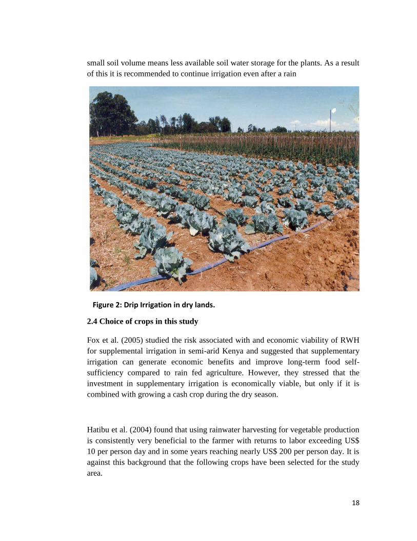
small soil volume means less available soil water storage for the plants. As a result
of this it is recommended to continue irrigation even after a rain
Figure 2: Drip Irrigation in dry lands.
2.4 Choice of crops in this study
Fox et al. (2005) studied the risk associated with and economic viability of RWH
for supplemental irrigation in semi-arid Kenya and suggested that supplementary
irrigation can generate economic benefits and improve long-term food self-
sufficiency compared to rain fed agriculture. However, they stressed that the
investment in supplementary irrigation is economically viable, but only if it is
combined with growing a cash crop during the dry season.
Hatibu et al. (2004) found that using rainwater harvesting for vegetable production
is consistently very beneficial to the farmer with returns to labor exceeding US$
10 per person day and in some years reaching nearly US$ 200 per person day. It is
against this background that the following crops have been selected for the study
area.
19
2.4.1 Tomato Cultivation
Tomato (Lycopersicon esculentum) is the second most important vegetable crop
after potato. Present world production is about 100 million tons fresh fruit from
3.7 million ha). Tomatoes are used in salads, cooked as a vegetable or used in
chutneys. Tomatoes are excellent sources of antioxidants, dietary fiber, minerals,
and vitamins. Fresh juices and its soup are becoming increasingly popular health-
drinks across the world. Lycopene antioxidant present in tomatoes is scientifically
found to be protective against cancers including colon, prostate, breast,
endometrial, lung, and pancreatic tumors. Fresh tomatoes are a good source of
vitamin C and potassium. This crop has high returns on investment (ROI), making
it suitable for farming business. Good quality tomatoes which have been carefully
handled command good market prices.
Climatic requirements: Tomatoes grow well in warm conditions and they are
fairly adaptable, but excessive humidity and temperatures reduce yields.
Nursery: Choose a nursery site where potatoes, eggplants, peppers and cape
gooseberries have not been grown for the last 3 years because of disease risk. A
seed rate of 100-200g will give you seedlings enough to plant 1 hectare. Sow the
seeds in drills 20 cm apart and 1cm deep. Thin out to 7cm apart latter in rows in
order to raise strong seedlings.
Manure: If soils are poor in organic matter, apply 10kg of well decomposed
manure per square meter prior to transplanting to improve yields of tomatoes.
Transplanting: This is carried out about one month after sowing seeds in the
nursery, or when the plants are about 10-15cm high. Select only the healthy strong
seedlings and plant at a spacing of 90cm x 60 cm. Transplant with soil attached to
the roots on a cloudy day or late in the evening.
Fertilizers: When transplanting, apply 200kg/ha of double super phosphate which
is equivalent to 5g/planting hole. Mix the fertilizer with the soil thoroughly to
avoid scorching, and when the plants are 25cm high Top dress with calcium
ammonium nitrate at a rate of 100kg per hectare. An application of calcium
ammonium nitrate at a rate of 200kg/ha 4 weeks later is beneficial.
Mulching and weeding: Mulch with dry trash to conserve moisture and keep
down soil temperatures. Keep the field free of weeds in order to reduce
competition for water and nutrients.
20
Pruning: Leave 2 main stems and pinch out the laterals as they grow every week.
When 6-8 trusses have formed, pinch out the growing tip. Pruning will encourage
growth of good sized marketable tomatoes. Remove the leaves close to the ground
to prevent the entry of blight and other fungal diseases disease.
Watering: water thoroughly 2-3 times every week.
Staking: This is done by pushing firmly into the ground a 2m stake for each plant.
Loosely tie the stem to the stake as the plant grows. Alternatively put a stout pole
in the ground every 4 meters and run two wires at a height of 2m and 0.15m from
the ground respectively. From the top wire run a string down for each plant to the
bottom wire. The plants can be carefully twisted around the string as they grow.
Harvesting: Fruit for fresh market should be slightly under ripe at harvesting time
for it to travel well to the market, while fruit for canning should be ripe.
Maturity period: Tomatoes mature in 3-4 months after transplanting depending on
variety and agro-ecological zone.
2.4.2 Cultivation of Capsicum Pepper
Capsicum pepper also known as sweet paper is the most popular and most widely
used condiment all over the world. Its fruits are consumed in fresh, dried or
processed form as table vegetable or spice. Capsicum peppers are extensively
pickled in salt and vinegar. Colour and flavour extracts are used in both the food
and feed industries, for example, ginger beer, hot sauces and poultry feed, as well
as for some pharmaceutical products. Sweet, non-pungent capsicum peppers are
widely used in the immature, green-mature or mature-mixed-colours stage as a
vegetable, especially in the temperate zones. Capsicum extracts show promise
against some crop pests.
Climate, soil and water management
Climatic requirements and cultural practices for production of sweet peppers and
chilies are the same. They also share a same complex of pests and diseases.
Capsicum peppers tend to tolerate shade conditions up to 45% of prevailing solar
radiation, although shade may delay flowering. Capsicum peppers grow best on
well-drained loamy soils at pH 5.5-6.8. They grow at a wide range of altitudes,
with rainfall between 600 and 1250 mm. severe flooding or drought is injurious to
most cultivars. Seeds germinate best at 25-30°C. Optimal temperatures for
21
productivity are between 18 and 30°C. C. frutescence are more tolerant to high
temperatures. Cooler night temperatures down to 15°C favour fruit setting,
although flowering will be delayed as temperatures drop below 25°C. Flower buds
will usually abort rather than develop to maturity if night temperatures reach 30°C.
Pollen viability is significantly reduced at temperatures above 30°C and below
15°C.
Propagation and planting
Capsicum peppers are propagated by seed. Seeds should be harvested from mature
fresh fruit after 2 weeks of ripening after harvest. Seeds remain viable for 2-3
years without special conservation methods if they are kept dry. They rapidly lose
viability if they are not properly stored especially at high temperature or humidity.
Seed dormancy may occur to a small extent, especially if seed is harvested from
under-ripe fruits. Some 200-800 g of seed is required per ha, depending on plant
density. When using own seeds, hot-water treat the seeds.
Seedbeds are usually covered with straw, leaves or protective tunnels. For better
production, seedlings should be transferred to seedling pots (plastic pots, paper
cups, banana leaf-rolls, etc.) when the cotyledons are fully expanded. Transplants
are planted out in the field at the 8-10 true leaf stage, usually 30-40 days after
sowing. Hardy transplants can be produced by restricting water and removing
shade protection, starting 4-7 days before transplanting. Transplanting should be
done during cloudy days or in the late afternoon, and should be followed
immediately by irrigation. Direct sowing in the field is practiced to a limited
extent. Capsicum peppers are well adapted to sole cropping and intercropping
systems. Capsicum peppers are often relay-cropped with tomatoes, shallots,
onions, garlic, okra, Brassica spp. and pulses. They also grow well among newly
established perennial crops.
Cultivars commonly grown in Kenya: Sweet pepper (C. annuum), California
Wonder, Yolo wonder, Emerald Giant, Ruby Giant
Husbandry Practices
Capsicum peppers thrive best if supplied with a generous amount of organic
matter. A reasonable recommendation is to supply 10-20 t/ha of organic matter.
General nutrient requirements are 130 kg/ha of N, 80 kg/ha of P and 110 kg/ha of
K. Nutrient availability is subject to soil type and environmental conditions, so
local recommendations vary. Manual weeding is usual for weed control. It is most
22
critical at the reproductive phase. Organic or plastic mulches are very effective for
weed control, and reflective mulches help to minimise insect vectors of plant
viruses. Staking can help minimise lodging. Capsicum peppers may be grown
under rain-fed or irrigated conditions. To avoid certain diseases, pests or
allelopathic damage, capsicum peppers should not be planted after other
solanaceous crops, sweet potato or jute.
Harvesting
Capsicum peppers are ready for harvest 3-6 weeks after flowering depending on
the fruit maturity desired. Green fruits are mature when firm, if gently squeezed
they make a characteristic popping sound. Harvesting is done by hand or with the
aid of a small knife.
Sweet capsicum peppers are often harvested at the green mature stage, although
sometimes they are harvested red. Assorted fruit colours such as yellow, orange,
chocolate and purple are also available in specialised markets. Hot capsicum
peppers are harvested green or red depending on their utilisation.
For the fresh market, fruits are harvested mature but firm, whereas capsicum
peppers sold as dried pods may be left to partially dry on the plants before
harvesting. Yields under irrigated conditions tend to be higher than for rain-fed
production, but vary with other management practices. Unless sold for the fresh
market, hot capsicum peppers can be sun-dried. Sun-drying usually takes place in
a vacant field or roadside, on mats or a well-swept area. In the sun, capsicum
peppers will dry adequately in 10-20 days, with frequent turning of fruits.
Steaming of hot and capsicum pepper before being sun-dried tends to improve the
appearance, making dried fruits look glossy.
2.4.3 Cabbage Cultivation
Cabbage is one of the most important vegetables grown for cooking and
use in salads in Kenya. The plant‘s scientific name is Brassica oleraceae and its
propagated from seed. The seed is widely available in seed stores across Kenya.
23
This vegetable is grown rain fed or under irrigated conditions. Cabbage is mainly
used for cooking, in vegetable salad and as plant matter for livestock feed. There
are several cabbage varieties in Kenya. Sugar loaf, Pructor F1, Gloria F1 hybrid
and Copenhagen market are considered as sweet tasting varieties. The most
popular are Gloria F1 hybrid, Copenhagen market and Pructor F1. Cabbage
varieties grown depend on market requirements and taste.
Climatic requirements:
Optimum temperatures for cabbage growing are 16-20ºC .At temperatures
above25ºC head formation is reduced. The vegetable has high water requirement
during growth period with 500mm rainfall considered optimal. Cabbage can grow
in altitude ranging from 800 to over 2,000 metres
Soils
Soils should be well drained, high in organic matter, high water holding capacity
with optimum ph of 6-6.5.
Crop duration
Healthy seedlings should be transplanted when they are about 4-6 we old or when
10-12cm high. Harvesting starts 3- 4months after transplanting and lasts 4-6
weeks. The vegetable is ready when heads are firm.3-4 wrapper leaves should be
left to cover the head and keep it fresh .Depending on variety, soil nutrient status,
2.5 Determination of Crop Water Requirements
Crop water requirement (CWR) can be defined as the total water needed for
evapotranspiration, from planting to harvest, for a given crop in a specific climate
regime, when adequate soil water is maintained by rainfall and/or irrigation so that
it does not limit plant growth and crop yield (Aquastat glossary).
For a plant to grow, water is necessary. Most water needs for crops grown in
season are met by rainfall. However, not all rain that falls is used by the crops.
Effective rainfall therefore is defined as the part of rainfall which is effectively
used by the crop after rainfall losses due to surface run off and deep percolation.
Effective rainfall is the rainfall that is used to determine crop irrigation
requirements with the following equation:
IRReq= ETcrop- Peff
24
Where;
IRReq= Irrigation requirement in (mm/day)
ETcrop= Crop evapotranspiration in (mm/day)
Peff= Effective rainfall in (mm)
There are four different methods used to calculate effective rainfall and these are:
Fixed Percentage, Dependable Rain, Empirical Formula, and USDA Soil
Conservation Service Method
Evaporation & Transpiration
In a cropped field water can be lost through two processes
1. Water can be lost from the soil surface and vegetation through a process called
evaporation (E), whereby liquid water is converted into water vapour and removed
from the evaporating surface. This process is affected by climate factors such as
solar radiation, air temperature, air humidity and wind speed where the
evaporating surface is the soil surface.
2. The second process of water loss is called transpiration (T), whereby liquid
water contained in plant tissues vaporizes into the atmosphere through small
openings in the plant leaf, called stomata. Transpiration, like direct evaporation,
depends on the energy supply, vapour pressure gradient and wind. Hence solar
radiation, air temperature, air humidity and wind parameters should be considered
when assessing transpiration.
The combination of these two separate processes, whereby water is lost on one
hand by evaporation from the soil surface and on the other hand by transpiration
from a plant, is called evapotranspiration (ET). Evaporation and transpiration
occur simultaneously and there is no easy way of distinguishing between the two
processes
Reference crop evapotranspiration (ETo)
This is the evapotranspiration from a reference surface not short of water and is
denoted by ETo. The reference surface is a hypothetical grass reference crop with
specific characteristics. The only factors affecting ETo are climatic parameters and
do not consider crop and soil factors. There are several methods of determining
25
reference crop evapotranspiration like the Pan Evaporation method, Blanney
Criddle method and Radiation method. However, FAO Penman-Monteith method
is now the sole recommended method for determining reference crop
evapotranspiration (ETo). This method overcomes the shortcomings of all other
previous empirical and semi empirical methods and provides ETo values that are
more consistent with actual crop water use data in all regions and climates.
Penman-Monteith Equation
The Penman-Monteith Equation is given by the following equation (FAO, 1998a):
ETo =0.408 Ä (Rn - G) + ãT + 273u2 (es - ea) Ä + ã (1 + 0.34 u2) Where:
ETo = Reference evapotranspiration (mm/day)
Rn = Net radiation at the crop surface (MJ/m2 per day)
G = Soil heat flux density (MJ/m2 per day)
T = Mean daily air temperature at 2 m height (°C)
u2 = Wind speed at 2 m height (m/sec)
es = Saturation vapour pressure (kPa)
ea = Actual vapour pressure (kPa)
es - ea = Saturation vapour pressure deficit (kPa)
Ä = Slope of saturation vapour pressure curve at temperature T (kPa/°C)
ã = Psychometric constant (kPa/°C)
Crop evapotranspiration under standard Conditions (ETc)
The crop evapotranspiration under standard conditions denoted as ETc, is the
evapotranspiration from disease-free, well-fertilized crop, grown in large fields
under optimum soil water conditions and achieving full production under the given
climatic conditions. The values of ETc and CWR(Crop Water Requirements) are
identical, whereby ETc refers to the amount of water lost through
evapotranspiration and CWR refers to the amount of water that is needed to
compensate for the loss.
ETc can be calculated from climatic data by directly integrating the effect of crop
characteristics into ETo.
26
Crop coefficient Kc
Experimentally determined ratios of ETc/ ETo, called crop coefficients (Kc), are
used to relate ETc to ETo as given in the following equation:
ETc = ETo x Kc
Where:
ETc = Crop evapotranspiration (mm/day)
ETo = Reference crop evapotranspiration (mm/day)
Kc = Crop coefficient
The Kc for a given crop changes over the growing period as the groundcover, crop
height and leaf area changes. There are four growth stages recognized for the
selection of Kc namely; initial stage, crop development stage, mid-season stage
and the late season stage. The variation of Kc for different crops is influenced by
weather factors and crop development stage.
The initial stage refers to the germination and early growth stage when the soil
surface is not or is hardly covered by the crop (Groundcover < 10%). The Kc at
this stage is referred to as the Initial stage (Kc initial).
The crop development stage: This is the stage from the end of the initial stage to
attainment of effective full groundcover (groundcover 70-80%). As the crop
develops and shades more and more of the ground, soil evaporation becomes more
restricted and transpiration becomes the dominant process. The Kc at this stage is
referred to as the crop development stage (Kc dev).
The mid-season stage: This is the stage from attainment of effective full
groundcover to the start of maturity, as indicated for example by discoloring of
leaves (as is the case for beans) or falling of leaves (for cotton). The Kc at this
stage is referred to as the mid-season stage (Kc mid). Mid-season stage is the
longest stage for perennial crops and for many annual crops, but it may be
relatively short for vegetables that are harvested fresh for their green vegetation.
At this stage, Kc reaches its maximum value. The value of Kc mid is relatively
constant for most growing and cultural conditions.
The late season stage: This stage runs from the start of maturity to harvest. The
calculation of Kc and ETo is presumed to end when the crop is harvested, dries out
27
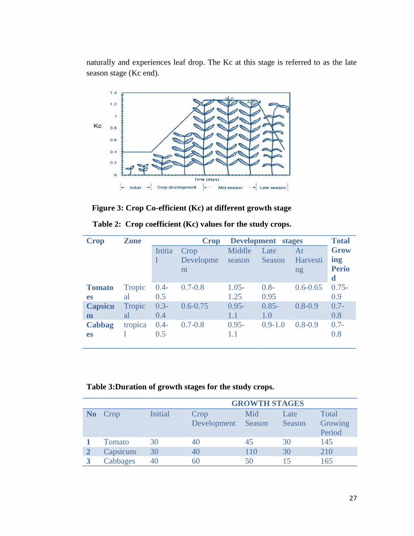
naturally and experiences leaf drop. The Kc at this stage is referred to as the late
season stage (Kc end).
Figure 3: Crop Co-efficient (Kc) at different growth stage
Table 2: Crop coefficient (Kc) values for the study crops.
Crop Zone Crop Development stages Total
Grow
ing
Perio
d
Initia
l
Crop
Developme
nt
Middle
season
Late
Season
At
Harvesti
ng
Tomato
es
Tropic
al
0.4-
0.5
0.7-0.8 1.05-
1.25
0.8-
0.95
0.6-0.65 0.75-
0.9
Capsicu
m
Tropic
al
0.3-
0.4
0.6-0.75 0.95-
1.1
0.85-
1.0
0.8-0.9 0.7-
0.8
Cabbag
es
tropica
l
0.4-
0.5
0.7-0.8 0.95-
1.1
0.9-1.0 0.8-0.9 0.7-
0.8
Table 3:Duration of growth stages for the study crops.
GROWTH STAGES
No Crop Initial Crop
Development
Mid
Season
Late
Season
Total
Growing
Period
1 Tomato 30 40 45 30 145
2 Capsicum 30 40 110 30 210
3 Cabbages 40 60 50 15 165

28
2.6 Planting Dates
The crops in this study are cash crops. As such it is important to time the crops to
go to the market when demand is high so that they can fetch good prices. During
the short rain season in Kenya production is usually lower because most farmers
do not grow the crops because of low rainfall. This results in high demand and
hence good market prices during the months of December to March. As a result of
this consideration 1st September was taken as the planting date in this study. Crops
planted on this day will also be able to take maximum use of little rains available.
29
3.0 MATERIAL AND METHODS
3.1 Description of the area of study
3.1.1 Location and climatic conditions
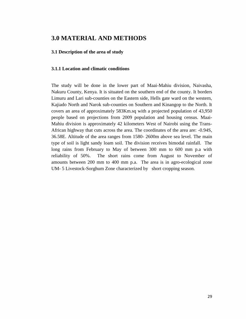
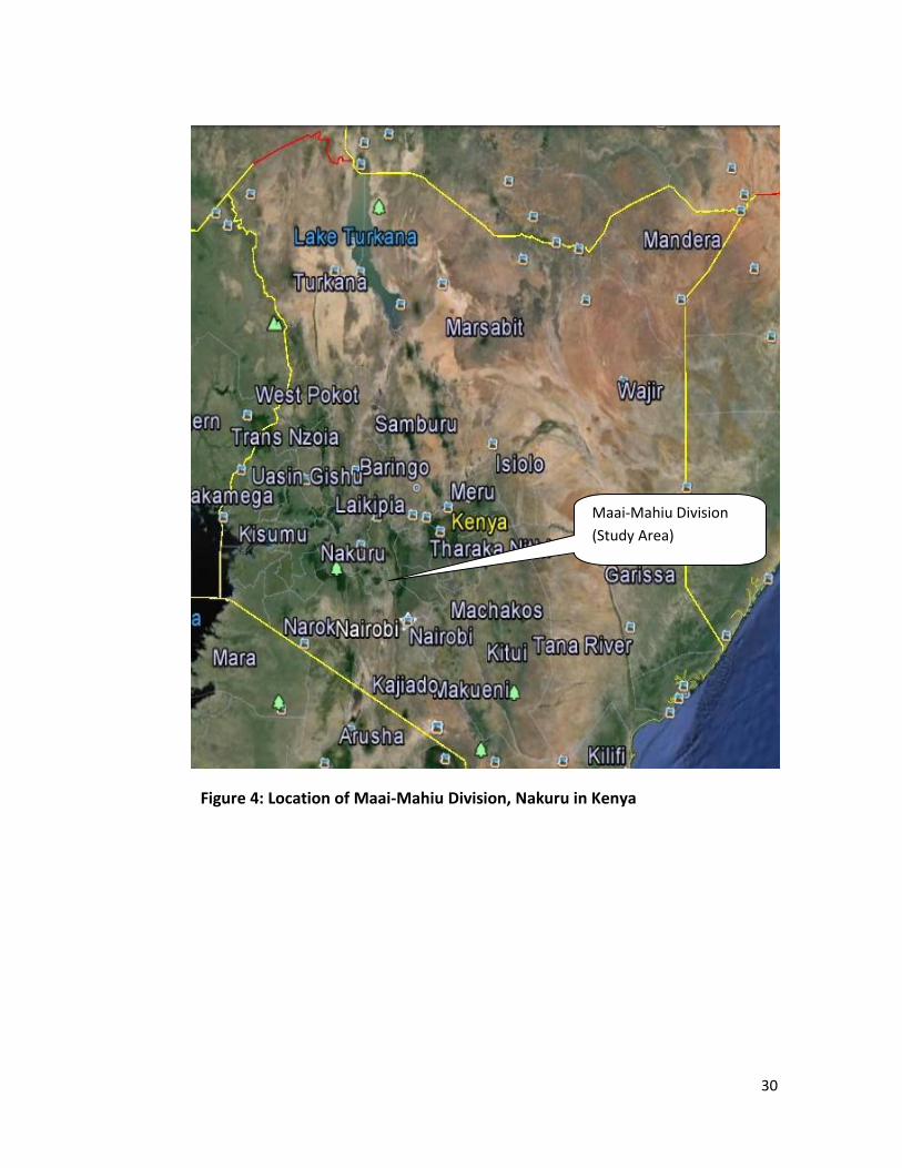
The study will be done in the lower part of Maai-Mahiu division, Naivasha,
Nakuru County, Kenya. It is situated on the southern end of the county. It borders
Limuru and Lari sub-counties on the Eastern side, Hells gate ward on the western,
Kajiado North and Narok sub-counties on Southern and Kinangop to the North. It
covers an area of approximately 583Km.sq with a projected population of 43,950
people based on projections from 2009 population and housing census. Maai-
Mahiu division is approximately 42 kilometers West of Nairobi using the Trans-
African highway that cuts across the area. The coordinates of the area are: -0.94S,
36.58E. Altitude of the area ranges from 1580- 2600m above sea level. The main
type of soil is light sandy loam soil. The division receives bimodal rainfall. The
long rains from February to May of between 300 mm to 600 mm p.a with
reliability of 50%. The short rains come from August to November of
amounts between 200 mm to 400 mm p.a. The area is in agro-ecological zone
UM- 5 Livestock-Sorghum Zone characterized by short cropping season.
30
Figure 4: Location of Maai-Mahiu Division, Nakuru in Kenya
Maai-Mahiu Division
(Study Area)
31
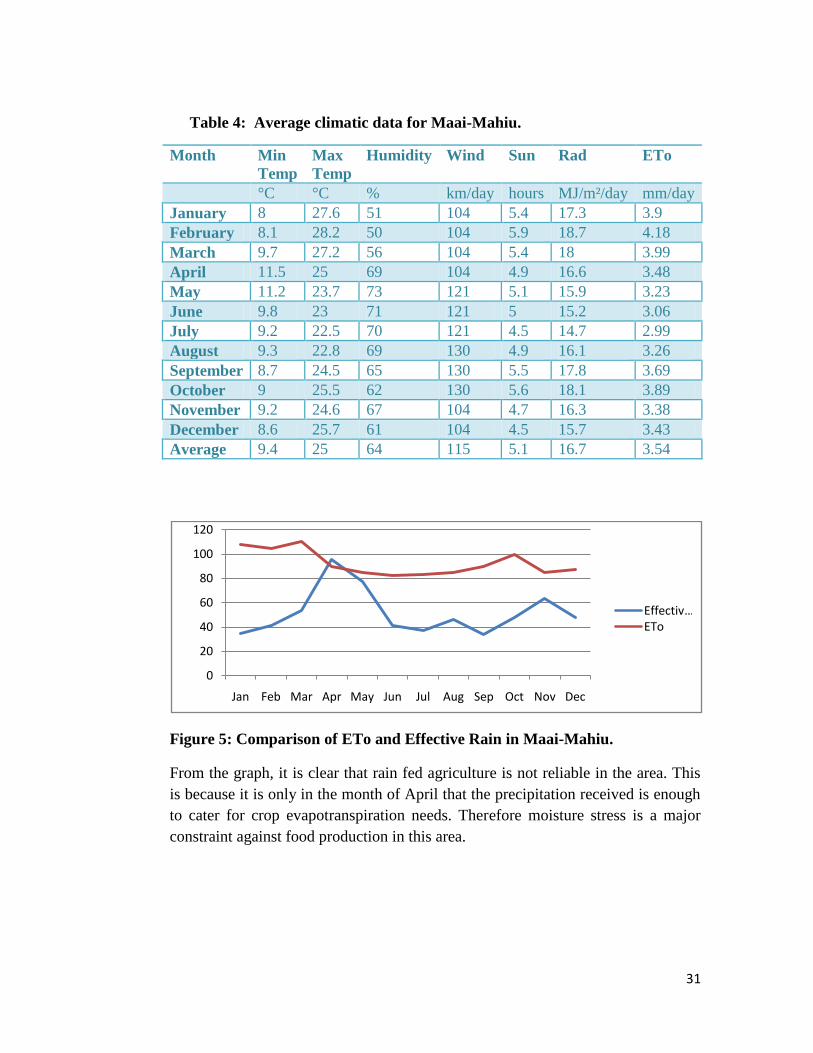
Table 4: Average climatic data for Maai-Mahiu.
Month Min
Temp
Max
Temp
Humidity Wind Sun Rad ETo
°C °C % km/day hours MJ/m²/day mm/day
January 8 27.6 51 104 5.4 17.3 3.9
February 8.1 28.2 50 104 5.9 18.7 4.18
March 9.7 27.2 56 104 5.4 18 3.99
April 11.5 25 69 104 4.9 16.6 3.48
May 11.2 23.7 73 121 5.1 15.9 3.23
June 9.8 23 71 121 5 15.2 3.06
July 9.2 22.5 70 121 4.5 14.7 2.99
August 9.3 22.8 69 130 4.9 16.1 3.26
September 8.7 24.5 65 130 5.5 17.8 3.69
October 9 25.5 62 130 5.6 18.1 3.89
November 9.2 24.6 67 104 4.7 16.3 3.38
December 8.6 25.7 61 104 4.5 15.7 3.43
Average 9.4 25 64 115 5.1 16.7 3.54
Figure 5: Comparison of ETo and Effective Rain in Maai-Mahiu.
From the graph, it is clear that rain fed agriculture is not reliable in the area. This
is because it is only in the month of April that the precipitation received is enough
to cater for crop evapotranspiration needs. Therefore moisture stress is a major
constraint against food production in this area.
0
20
40
60
80
100
120
Jan Feb Mar Apr May Jun Jul Aug Sep Oct Nov Dec
Effectiv…ETo
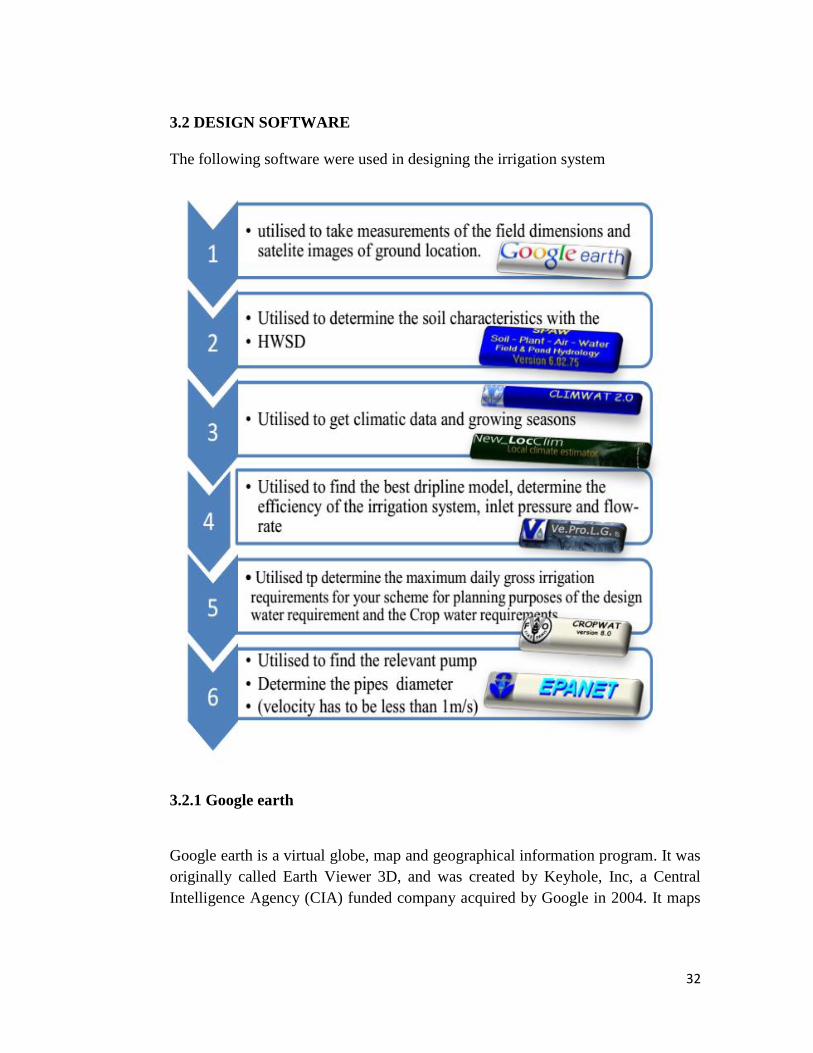
32
3.2 DESIGN SOFTWARE
The following software were used in designing the irrigation system
3.2.1 Google earth
Google earth is a virtual globe, map and geographical information program. It was
originally called Earth Viewer 3D, and was created by Keyhole, Inc, a Central
Intelligence Agency (CIA) funded company acquired by Google in 2004. It maps
33
the Earth by the superimposition of images obtained from satellite imagery, aerial
photography and GIS 3D globe
This program was used to locate, dimension and draw the field layout on
the ground shown clearly by a satellite image of the thesis plot. Data used
for software VEPROL G about the field dimensions was also obtained using
this program. Data used for the design of the pond like the catchment slope
and the total catchment area for the water harvesting was also obtained using
this program.
3.2.2 Harmonised World soil Database (HWSD)
Harmonised World soil Database is a 30 arc-second raster database with over
16000 different soil mapping units that combines existing regional and
national updates of soil information worldwide. The HWSD contributes
sound scientific knowledge for planning sustainable expansion of agricultural
production to achieve food security and provides information for national
and international policymakers in addressing emerging problems of land
competition for food production, bio-energy demand and threats to
biodiversity (FAO, 2009).
This was used to obtain the soil type of the study area. The Harmonized
World soil Database Viewer Version 1.2 done by FAO, Chinese academy of
sciences, International Institute for Applied systems analysis. International
soil reference and Information Center and the Joint research center of the
European Commission. The results from the HWSD viewer were entered into
the soil textural triangle to be able to generate the CROPWAT input details of
the TAW and max rain infiltration rate which is directly related to the
hydraulic conductivity obtained from the textural triangle.
3.2.3 Soil water characteristics
This program estimates soil water tension, conductivity and water holding
capability based on the soil texture, organic matter, gravel content, salinity, and
compaction.
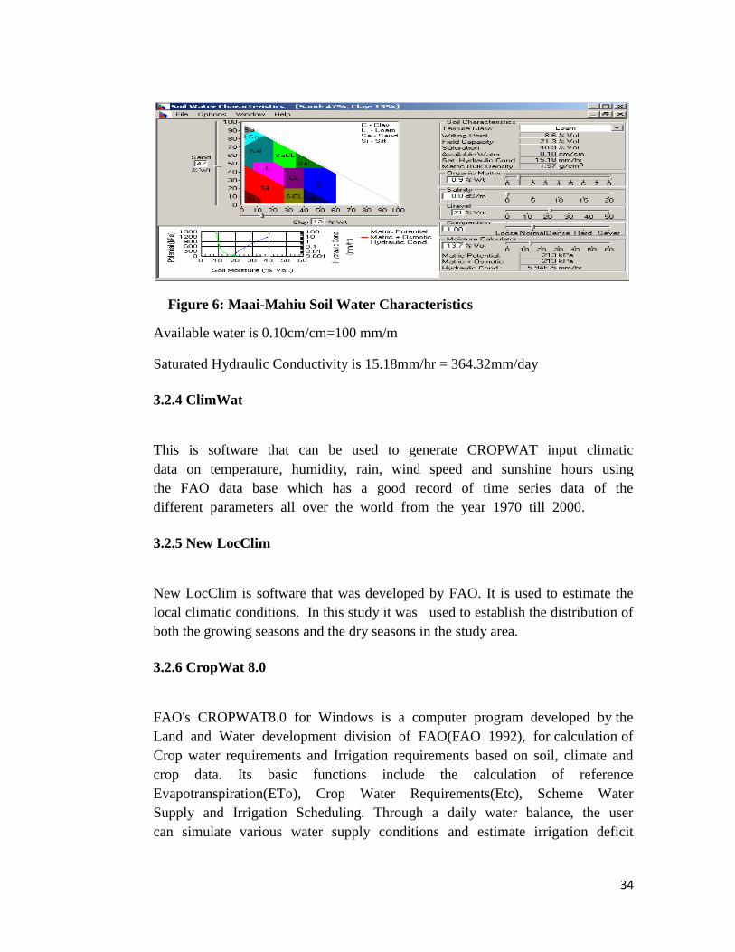
34
Figure 6: Maai-Mahiu Soil Water Characteristics
Available water is 0.10cm/cm=100 mm/m
Saturated Hydraulic Conductivity is 15.18mm/hr = 364.32mm/day
3.2.4 ClimWat
This is software that can be used to generate CROPWAT input climatic
data on temperature, humidity, rain, wind speed and sunshine hours using
the FAO data base which has a good record of time series data of the
different parameters all over the world from the year 1970 till 2000.
3.2.5 New LocClim
New LocClim is software that was developed by FAO. It is used to estimate the
local climatic conditions. In this study it was used to establish the distribution of
both the growing seasons and the dry seasons in the study area.
3.2.6 CropWat 8.0
FAO's CROPWAT8.0 for Windows is a computer program developed by the
Land and Water development division of FAO(FAO 1992), for calculation of
Crop water requirements and Irrigation requirements based on soil, climate and
crop data. Its basic functions include the calculation of reference
Evapotranspiration(ETo), Crop Water Requirements(Etc), Scheme Water
Supply and Irrigation Scheduling. Through a daily water balance, the user
can simulate various water supply conditions and estimate irrigation deficit
35
and rainfall efficiencies. Typical applications of the water balance include
the development of irrigation schedules for various crops and various
irrigation methods, the evaluation practices as well as rain fed production
and drought effects.
3.2.7 Epanet
This is software that models water distribution piping systems. It is a public
domain software that may be freely copied and distributed. It‘s based on
Windows 95/98/NT/XP program. EPANET performs extended period simulation
of the water movement and quality behavior within pressurized pipe networks.
EPANET was developed by the Water Supply and Water Resources
Division (formerly the Drinking Water Research Division) of the U.S.
Environmental Protection Agency‘s National Risk Management Research
3.2.8 Ve.pro.LG.s
This is application software that evaluates dimensioning and design systems of
drip irrigation. This evaluation is aimed at increasing the uniformity of
distribution of irrigation in order to save water and reduce energy
consumption. The name is derived from the initials of ―Verification and
Design of drip lines and areas of plant stems‖ (Ve.pro.LG.s)
The first version was released in 2003 and it brought a substantial evolution,
being able to assess the functioning of entire planting areas and also extend
the application range of the horticultural industry and tree crops, even when grown
on sloping ground elevation along the line.
3.3 Source of water for irrigation.
In this study, the source of water is proposed water harvesting earth dam
constructed on the upper side of the catchment. The study will help in assessing
the potential of rainwater harvesting for crop production in the area by
optimization of design parameters such as analysis of rainfall, water demand,
catchment area and storage capacity.
36
3.4 Estimating runoff using the runoff curve number method.
3.4.1 Design parameters
Surface runoff refers to the water flowing on the surface of the land as overland
sheet flow or channel flow or both. Water flows from higher elevations to lower
elevations due to gravitational forces. Small streams eventually combine to form
rivers that finally drain into the seas or oceans to complete the hydrologic cycle.
Runoff consists of three components: surface flow, interflow, and groundwater
flow. Surface runoff is produced by the effective rainfall and is equal to the total
rainfall minus hydrologic abstractions. Surface flow is also known as direct runoff
and produces large flows in rivers due to its relatively shorter time of
concentration (V. P. Singh et al 2003).
Low adoption of rainwater harvesting technology in Arid and Semiarid Lands
(ASAL), has been caused by many factors key among them lack of appropriate
technical designs. It is therefore important to optimize on Rain Water Catchment
Systems (RWCS). To address this problem, this study focuses on using
hydrological criteria for determining RWCS design parameters, especially storage
capacity and catchment area, using historical rainfall records of a rainfall station
near the area of study. Rainfall is the main input parameter in the design of
RWCS. Therefore, appropriate rainfall analysis is a prerequisite in the
determination of design parameters, mainly storage capacity and catchment area.
The runoff curve number (also called a curve number or simply CN) is an
empirical parameter used in hydrology for predicting direct runoff or infiltration
from rainfall excess. The curve number method was developed by the USDA
Natural Resources Conservation Service, which was formerly called the Soil
Conservation Service or SCS — the number is still popularly known as a
"SCS runoff curve number" in the literature. The runoff curve number was
developed from an empirical analysis of runoff from small catchments and
hill slope plots monitored by the USDA. It is widely used and is an
efficient method for determining the approximate amount of direct runoff from
a rainfall event in particular area.
The runoff curve number is based on the area's hydrologic soil group, land
use, treatment and hydrologic condition. Urban hydrology for small watersheds
Technical Release 55 (TR-55) (Second Edition ed.) of the United States
37
Department of Agriculture indicate the runoff curve numbers for characteristic
land cover descriptions and a hydrologic soil group.
The runoff equation is:
Where
Q is runoff ([L]; in)
P is rainfall ([L]; in)
S is the potential maximum soil moisture retention after runoff begins ([L]; in)
Ia- is the initial abstraction ([L]; in), or the amount of water before runoff, such
as infiltration, or rainfall interception by vegetation; historically, it has
generally been assumed that .Recent research has found that
may be a more appropriate and accurate relationship.
Ia-The runoff curve number, CN, is then related
CN has a range from 30 to 100; lower numbers indicate low runoff potential while
larger numbers are for increasing runoff potential. The lower the curve number,
the more permeable the soil is. As can be seen in the curve number equation,
runoff cannot begin until the initial abstraction has been met.
3.4.2 Curve Number Selection
The NRCS curve number is related to soil type, soil infiltration capability, land
use, and the depth of the seasonal high water table. To account for different soils'
ability to infiltrate, NRCS has divided soils into four hydrologic soil groups
(HSGs). They are defined as follows.
HSG Group A (low runoff potential): Soils with high infiltration rates even
when thoroughly wetted. These consist chiefly of deep, well-drained sands
and gravels. These soils have a high rate of water transmission (final
infiltration rate greater than 0.3 in. /h).
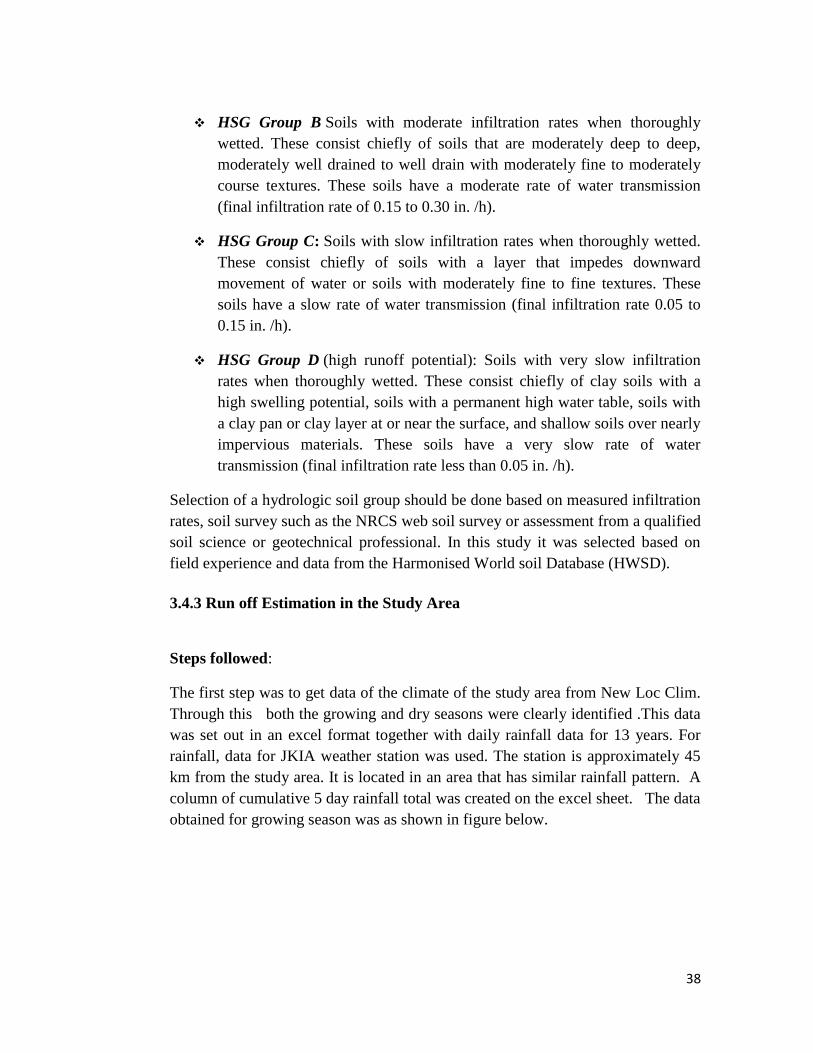
38
HSG Group B Soils with moderate infiltration rates when thoroughly
wetted. These consist chiefly of soils that are moderately deep to deep,
moderately well drained to well drain with moderately fine to moderately
course textures. These soils have a moderate rate of water transmission
(final infiltration rate of 0.15 to 0.30 in. /h).
HSG Group C: Soils with slow infiltration rates when thoroughly wetted.
These consist chiefly of soils with a layer that impedes downward
movement of water or soils with moderately fine to fine textures. These
soils have a slow rate of water transmission (final infiltration rate 0.05 to
0.15 in. /h).
HSG Group D (high runoff potential): Soils with very slow infiltration
rates when thoroughly wetted. These consist chiefly of clay soils with a
high swelling potential, soils with a permanent high water table, soils with
a clay pan or clay layer at or near the surface, and shallow soils over nearly
impervious materials. These soils have a very slow rate of water
transmission (final infiltration rate less than 0.05 in. /h).
Selection of a hydrologic soil group should be done based on measured infiltration
rates, soil survey such as the NRCS web soil survey or assessment from a qualified
soil science or geotechnical professional. In this study it was selected based on
field experience and data from the Harmonised World soil Database (HWSD).
3.4.3 Run off Estimation in the Study Area
Steps followed:
The first step was to get data of the climate of the study area from New Loc Clim.
Through this both the growing and dry seasons were clearly identified .This data
was set out in an excel format together with daily rainfall data for 13 years. For
rainfall, data for JKIA weather station was used. The station is approximately 45
km from the study area. It is located in an area that has similar rainfall pattern. A
column of cumulative 5 day rainfall total was created on the excel sheet. The data
obtained for growing season was as shown in figure below.
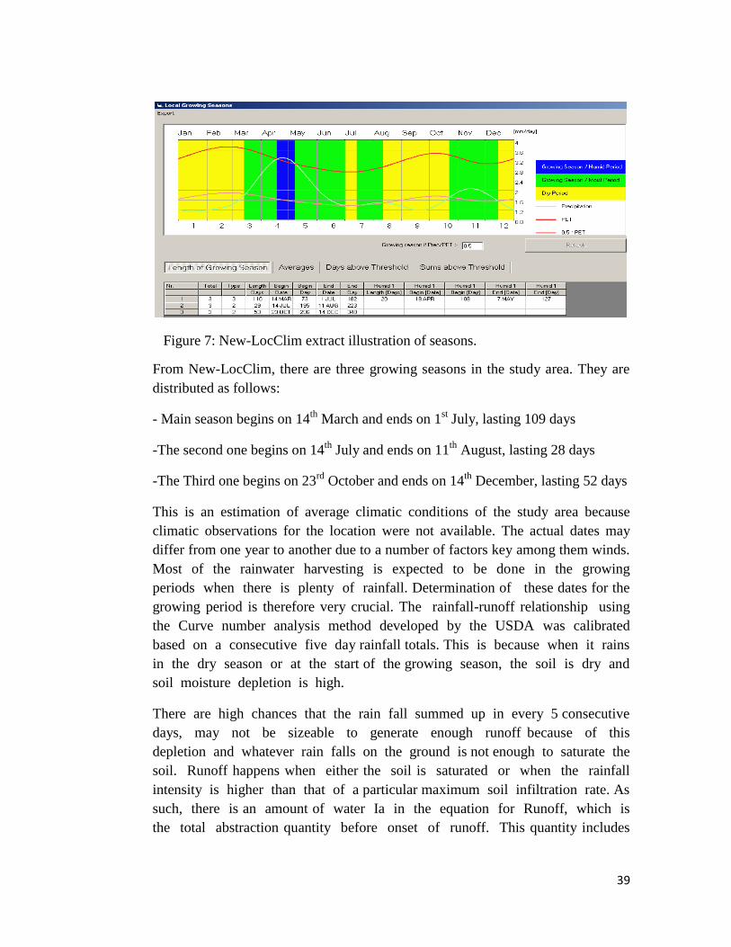
39
Figure 7: New-LocClim extract illustration of seasons.
From New-LocClim, there are three growing seasons in the study area. They are
distributed as follows:
- Main season begins on 14th
March and ends on 1st July, lasting 109 days
-The second one begins on 14th
July and ends on 11th
August, lasting 28 days
-The Third one begins on 23rd
October and ends on 14th
December, lasting 52 days
This is an estimation of average climatic conditions of the study area because
climatic observations for the location were not available. The actual dates may
differ from one year to another due to a number of factors key among them winds.
Most of the rainwater harvesting is expected to be done in the growing
periods when there is plenty of rainfall. Determination of these dates for the
growing period is therefore very crucial. The rainfall-runoff relationship using
the Curve number analysis method developed by the USDA was calibrated
based on a consecutive five day rainfall totals. This is because when it rains
in the dry season or at the start of the growing season, the soil is dry and
soil moisture depletion is high.
There are high chances that the rain fall summed up in every 5 consecutive
days, may not be sizeable to generate enough runoff because of this
depletion and whatever rain falls on the ground is not enough to saturate the
soil. Runoff happens when either the soil is saturated or when the rainfall
intensity is higher than that of a particular maximum soil infiltration rate. As
such, there is an amount of water Ia in the equation for Runoff, which is
the total abstraction quantity before onset of runoff. This quantity includes
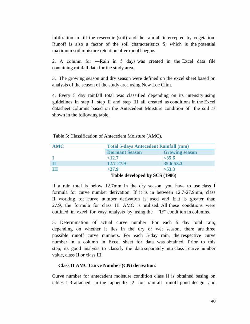
40
infiltration to fill the reservoir (soil) and the rainfall intercepted by vegetation.
Runoff is also a factor of the soil characteristics S; which is the potential
maximum soil moisture retention after runoff begins.
2. A column for ―Rain in 5 days was created in the Excel data file
containing rainfall data for the study area.
3. The growing season and dry season were defined on the excel sheet based on
analysis of the season of the study area using New Loc Clim.
4. Every 5 day rainfall total was classified depending on its intensity using
guidelines in step I, step II and step III all created as conditions in the Excel
datasheet columns based on the Antecedent Moisture condition of the soil as
shown in the following table.
Table 5: Classification of Antecedent Moisture (AMC).
AMC Total 5-days Antecedent Rainfall (mm)
Dormant Season Growing season
I <12.7 <35.6
II 12.7-27.9 35.6-53.3
III >27.9 >53.3
Table developed by SCS (1986)
If a rain total is below 12.7mm in the dry season, you have to use class I
formula for curve number derivation. If it is in between 12.7-27.9mm, class
II working for curve number derivation is used and If it is greater than
27.9, the formula for class III AMC is utilised. All these conditions were
outlined in excel for easy analysis by using the―‖IF‖ condition in columns.
5. Determination of actual curve number: For each 5 day total rain;
depending on whether it lies in the dry or wet season, there are three
possible runoff curve numbers. For each 5-day rain, the respective curve
number in a column in Excel sheet for data was obtained. Prior to this
step, its good analysis to classify the data separately into class I curve number
value, class II or class III.
Class II AMC Curve Number (CN) derivation:
Curve number for antecedent moisture condition class II is obtained basing on
tables 1-3 attached in the appendix 2 for rainfall runoff pond design and

41
summarized as shown in the table 7 below. These curve numbers are derived
using soil type and description of Land use.
Class I curve number is derived by using equation
Any 5 day rainfall that is below 35.6mm , it‘s curve number is obtained by
using equation for class I.
Class III curve number is derived by using equation;
6. Class I,II and III curve numbers were then used to classify each
individual 5 day rain by giving it any of the curve numbers in those
classes where it belonged.—either class I, II or III. A column for the
5 day rain curve number was created.
7. S, the potential maximum soil moisture retention after runoff begins was
obtained and fixed in a column of the excel sheet. . It is given by equation below.
CN is the final obtained Runoff curve number obtained in step 6.
8. Ia, the total abstraction quantity before onset of runoff was calculated and a
column created in the Excel sheet.
Ia = 0.2*S. Run off equation applies when >0.2S (Ia)
9. Individual values of Rainfall Runoff were computed using the equation below
(p>0.2S)
where
Q is runoff ([L]; mm)
P is rainfall ([L]; mm)
S is the potential maximum soil moisture retention after runoff
begins ([L]; mm)
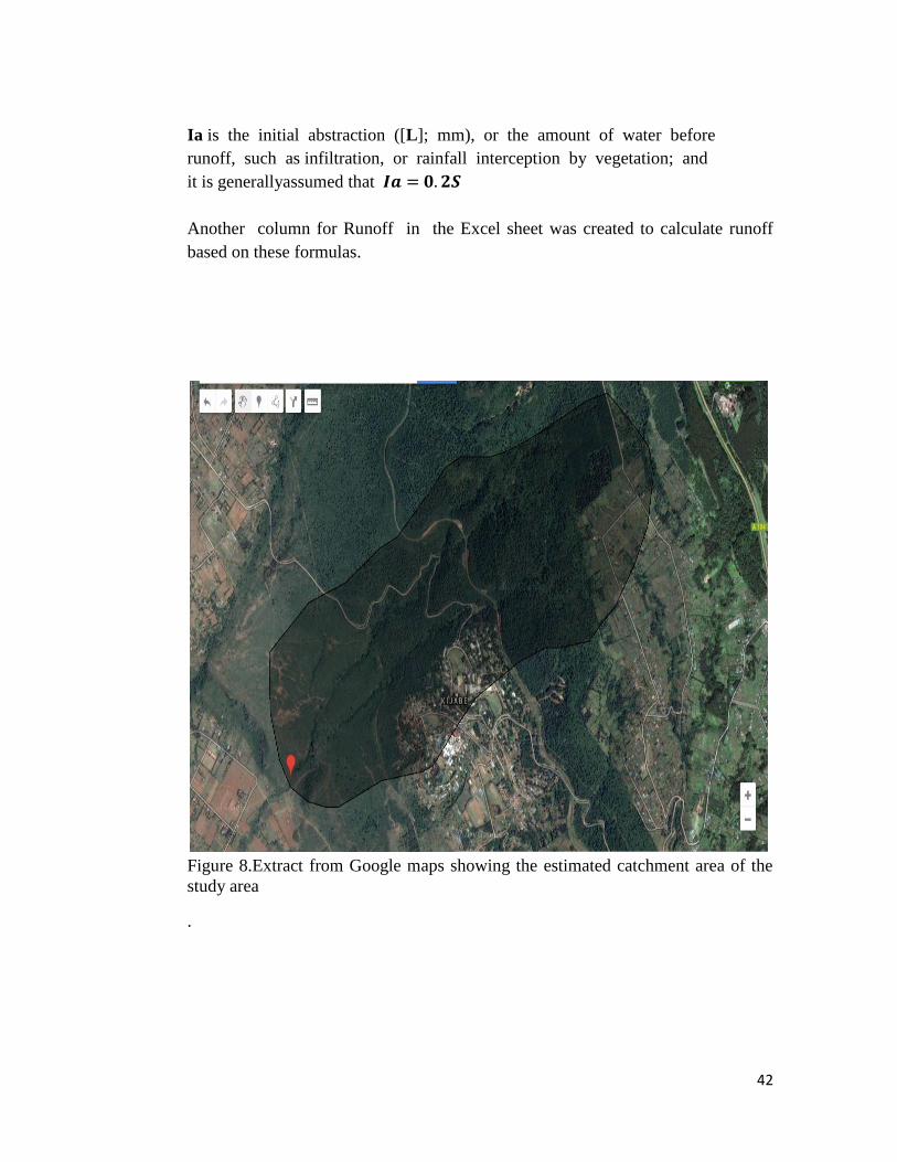
42
Ia is the initial abstraction ([L]; mm), or the amount of water before
runoff, such as infiltration, or rainfall interception by vegetation; and
it is generallyassumed that
Another column for Runoff in the Excel sheet was created to calculate runoff
based on these formulas.
Figure 8.Extract from Google maps showing the estimated catchment area of the
study area
.
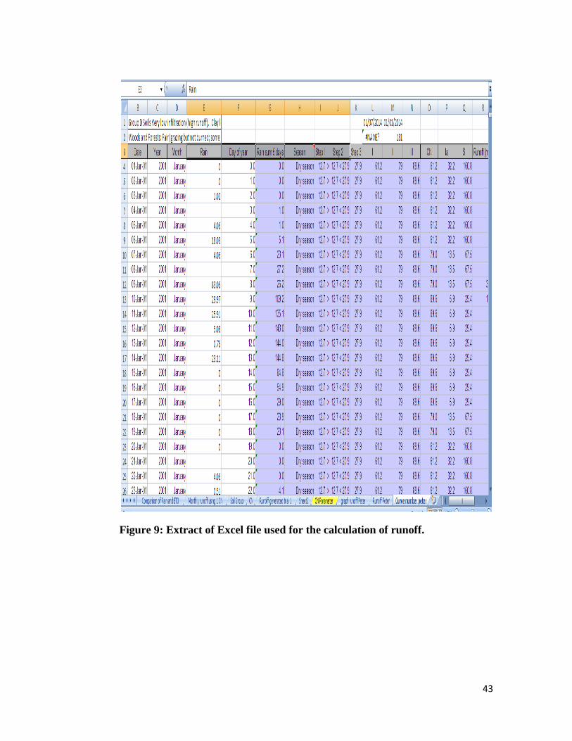
43
Figure 9: Extract of Excel file used for the calculation of runoff.
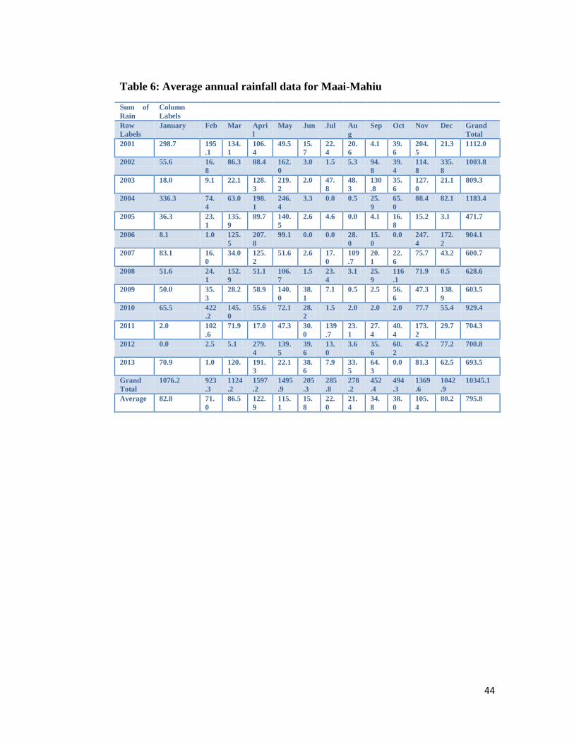
44
Table 6: Average annual rainfall data for Maai-Mahiu
Sum of
Rain
Column
Labels
Row
Labels
January Feb Mar Apri
l
May Jun Jul Au
g
Sep Oct Nov Dec Grand
Total
2001 298.7 195
.1
134.
1
106.
4
49.5 15.
7
22.
4
20.
6
4.1 39.
6
204.
5
21.3 1112.0
2002 55.6 16.
8
86.3 88.4 162.
0
3.0 1.5 5.3 94.
8
39.
4
114.
8
335.
8
1003.8
2003 18.0 9.1 22.1 128.
3
219.
2
2.0 47.
8
48.
3
130
.8
35.
6
127.
0
21.1 809.3
2004 336.3 74.
4
63.0 198.
1
246.
4
3.3 0.0 0.5 25.
9
65.
0
88.4 82.1 1183.4
2005 36.3 23.
1
135.
9
89.7 140.
5
2.6 4.6 0.0 4.1 16.
8
15.2 3.1 471.7
2006 8.1 1.0 125.
5
207.
8
99.1 0.0 0.0 28.
0
15.
0
0.0 247.
4
172.
2
904.1
2007 83.1 16.
0
34.0 125.
2
51.6 2.6 17.
0
109
.7
20.
1
22.
6
75.7 43.2 600.7
2008 51.6 24.
1
152.
9
51.1 106.
7
1.5 23.
4
3.1 25.
9
116
.1
71.9 0.5 628.6
2009 50.0 35.
3
28.2 58.9 140.
0
38.
1
7.1 0.5 2.5 56.
6
47.3 138.
9
603.5
2010 65.5 422
.2
145.
0
55.6 72.1 28.
2
1.5 2.0 2.0 2.0 77.7 55.4 929.4
2011 2.0 102
.6
71.9 17.0 47.3 30.
0
139
.7
23.
1
27.
4
40.
4
173.
2
29.7 704.3
2012 0.0 2.5 5.1 279.
4
139.
5
39.
6
13.
0
3.6 35.
6
60.
2
45.2 77.2 700.8
2013 70.9 1.0 120.
1
191.
3
22.1 38.
6
7.9 33.
5
64.
3
0.0 81.3 62.5 693.5
Grand
Total
1076.2 923
.3
1124
.2
1597
.2
1495
.9
205
.3
285
.8
278
.2
452
.4
494
.3
1369
.6
1042
.9
10345.1
Average 82.8 71.
0
86.5 122.
9
115.
1
15.
8
22.
0
21.
4
34.
8
38.
0
105.
4
80.2 795.8
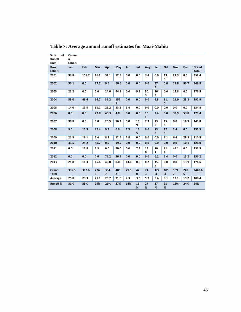
45
Table 7: Average annual runoff estimates for Maai-Mahiu
Sum of Runoff (mm)
Column Labels
Row Labels
Jan Feb Mar Apr May Jun Jul Aug Sep Oct Nov Dec Grand Total
2001 93.8 158.7 16.2 32.1 12.5 0.0 0.0 3.4 0.0 13.5
27.3 0.0 357.4
2002 30.1 0.0 17.7 9.6 60.6 0.0 0.0 0.0 27.2
0.0 13.8 90.7 249.8
2003 22.2 0.0 0.0 24.0 44.5 0.0 9.2 30.3
26.5
0.0 19.8 0.0 176.5
2004 59.0 46.6 16.7 36.2 152.5
0.0 0.0 0.0 6.8 31.0
21.0 23.2 392.9
2005 14.0 13.5 55.2 25.2 23.5 3.4 0.0 0.0 0.0 0.0 0.0 0.0 134.8
2006 0.0 0.0 27.8 46.3 4.8 0.0 0.0 10.1
3.4 0.0 33.9 53.0 179.4
2007 30.8 0.0 0.0 26.5 16.3 0.0 16.9
7.3 13.5
15.6
0.0 16.9 143.8
2008 9.0 13.5 42.4 9.3 0.0 7.3 13.5
0.0 13.0
22.0
3.4 0.0 133.5
2009 21.3 16.1 3.4 8.3 12.6 5.8 0.0 0.0 0.0 8.1 6.4 28.5 110.5
2010 33.5 24.2 40.7 0.0 19.5 0.0 0.0 0.0 0.0 0.0 0.0 10.1 128.0
2011 0.0 13.8 9.3 0.0 20.0 0.0 7.3 15.0
10.1
11.8
44.1 0.0 131.5
2012 0.0 0.0 0.0 77.2 36.3 0.0 0.0 0.0 6.2 3.4 0.0 13.2 136.2
2013 21.8 16.3 45.6 40.0 0.0 13.0 0.0 8.2 15.7
0.0 0.0 13.9 174.6
Grand Total
335.5 302.6 274.9
334.7
403.2
29.5 47.0
74.3
122.4
105.4
169.7
249.5
2448.6
Average 25.8 23.3 21.1 25.7 31.0 2.3 3.6 5.7 9.4 8.1 13.1 19.2 188.4
Runoff % 31% 33% 24% 21% 27% 14% 16%
27%
27%
21%
12% 24% 24%
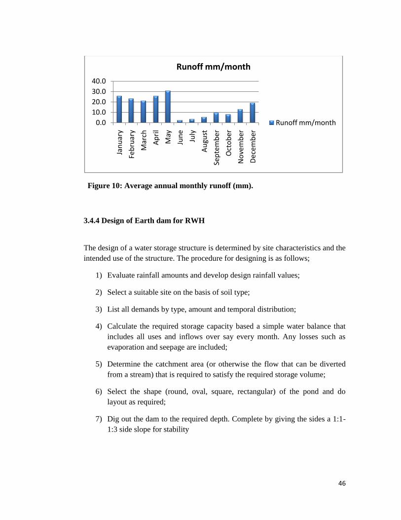
46
Figure 10: Average annual monthly runoff (mm).
3.4.4 Design of Earth dam for RWH
The design of a water storage structure is determined by site characteristics and the
intended use of the structure. The procedure for designing is as follows;
1) Evaluate rainfall amounts and develop design rainfall values;
2) Select a suitable site on the basis of soil type;
3) List all demands by type, amount and temporal distribution;
4) Calculate the required storage capacity based a simple water balance that
includes all uses and inflows over say every month. Any losses such as
evaporation and seepage are included;
5) Determine the catchment area (or otherwise the flow that can be diverted
from a stream) that is required to satisfy the required storage volume;
6) Select the shape (round, oval, square, rectangular) of the pond and do
layout as required;
7) Dig out the dam to the required depth. Complete by giving the sides a 1:1-
1:3 side slope for stability
0.0
10.0
20.0
30.0
40.0
Jan
uar
y
Feb
ruar
y
Mar
ch
Ap
ril
May
Jun
e
July
Au
gust
Sep
tem
ber
Oct
ob
er
No
vem
ber
Dec
emb
er
Runoff mm/month
Runoff mm/month
47
8) Design any other required structures such as diversion weir, conveyance
channel and spillway. An engineer should be consulted if in doubt about
these structures, their specifications or their design;
9) Select the type seepage and evaporation management methods;
10) Provide a monitoring system that traces the available water volume at any
time;
11) Fence the pond to provide security for people and livestock.
The selection of the shape should be done more carefully. Complicated shapes
such as ellipses can be more difficult to handle during volume calculations. But
squares and rectangular and circular shapes are quite easy to use and are
recommended.
3.4.5 Reducing Dam Water Losses
Most structures used in water storage have a number of common problems key
among them evaporation and seepage losses. Siltation can also be a problem.
However this can easily be tackled by regular maintenance and ensuring that water
inflows are devoid of excessive soil materials. But evaporation and seepage are
more serious.
Due to high temperatures, ponds in ASAL normally lose a lot of water through
evaporation. There are some technical solutions, but most of these are expensive to
implement.
A shade or a roof can be very effective in reducing evaporation through drastic
reduction in direct solar heating. Evaporation reduction can also be achieved by
placing wood chips which float on water and cover the water surface. It would be
expected that these methods can reduce evaporation losses by at least 95%. With
regard to seepage, the first intervention is to avoid making dams in soils with high
permeability. The second point is to evaluate possibilities of using a relatively
impervious material at the bottom of the pond. Clay blankets are effective but the
material may not be available on site. A plastic lining is now quite common. There
are special plastics capable of withstanding ultraviolet rays, but these are more
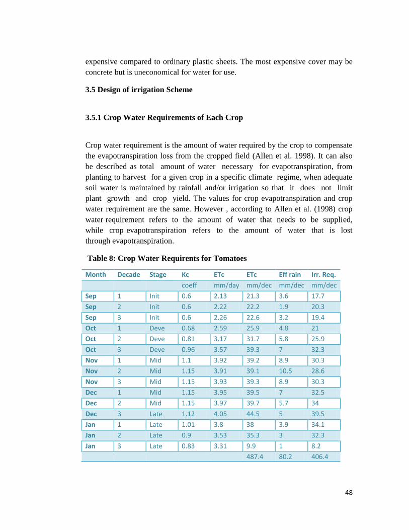
48
expensive compared to ordinary plastic sheets. The most expensive cover may be
concrete but is uneconomical for water for use.
3.5 Design of irrigation Scheme
3.5.1 Crop Water Requirements of Each Crop
Crop water requirement is the amount of water required by the crop to compensate
the evapotranspiration loss from the cropped field (Allen et al. 1998). It can also
be described as total amount of water necessary for evapotranspiration, from
planting to harvest for a given crop in a specific climate regime, when adequate
soil water is maintained by rainfall and/or irrigation so that it does not limit
plant growth and crop yield. The values for crop evapotranspiration and crop
water requirement are the same. However , according to Allen et al. (1998) crop
water requirement refers to the amount of water that needs to be supplied,
while crop evapotranspiration refers to the amount of water that is lost
through evapotranspiration.
Table 8: Crop Water Requirents for Tomatoes
Month Decade Stage Kc ETc ETc Eff rain Irr. Req.
coeff mm/day mm/dec mm/dec mm/dec
Sep 1 Init 0.6 2.13 21.3 3.6 17.7
Sep 2 Init 0.6 2.22 22.2 1.9 20.3
Sep 3 Init 0.6 2.26 22.6 3.2 19.4
Oct 1 Deve 0.68 2.59 25.9 4.8 21
Oct 2 Deve 0.81 3.17 31.7 5.8 25.9
Oct 3 Deve 0.96 3.57 39.3 7 32.3
Nov 1 Mid 1.1 3.92 39.2 8.9 30.3
Nov 2 Mid 1.15 3.91 39.1 10.5 28.6
Nov 3 Mid 1.15 3.93 39.3 8.9 30.3
Dec 1 Mid 1.15 3.95 39.5 7 32.5
Dec 2 Mid 1.15 3.97 39.7 5.7 34
Dec 3 Late 1.12 4.05 44.5 5 39.5
Jan 1 Late 1.01 3.8 38 3.9 34.1
Jan 2 Late 0.9 3.53 35.3 3 32.3
Jan 3 Late 0.83 3.31 9.9 1 8.2
487.4 80.2 406.4
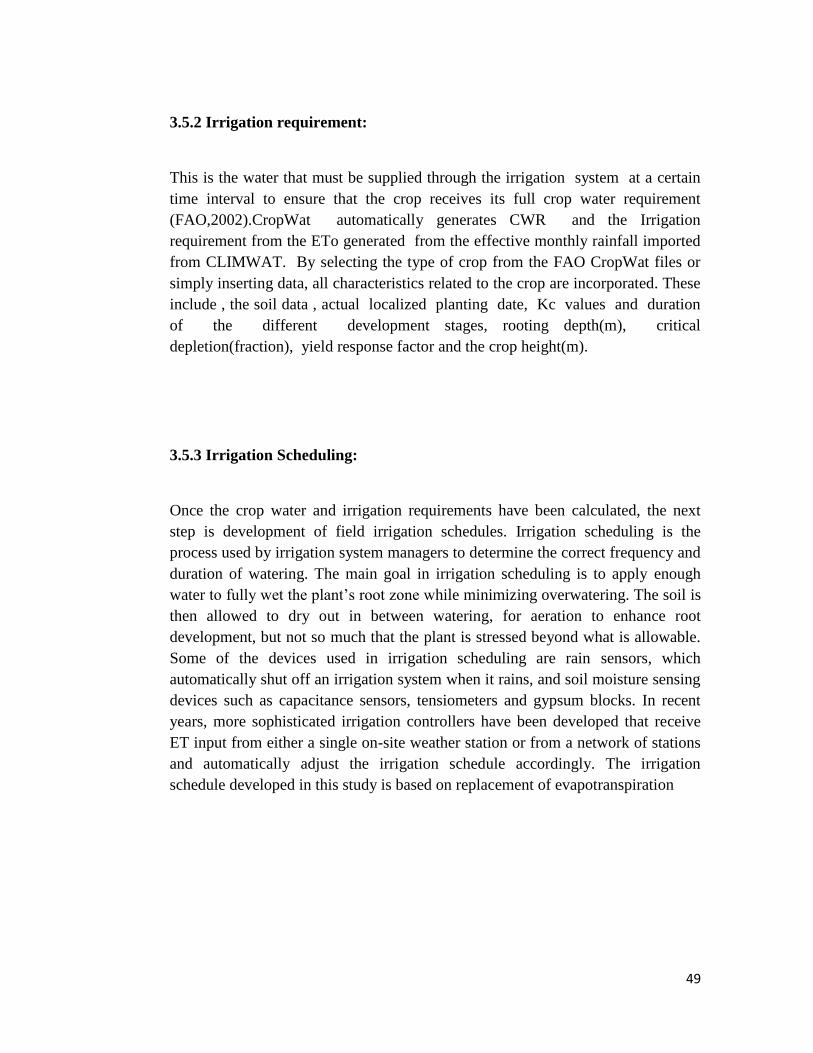
49
3.5.2 Irrigation requirement:
This is the water that must be supplied through the irrigation system at a certain
time interval to ensure that the crop receives its full crop water requirement
(FAO,2002).CropWat automatically generates CWR and the Irrigation
requirement from the ETo generated from the effective monthly rainfall imported
from CLIMWAT. By selecting the type of crop from the FAO CropWat files or
simply inserting data, all characteristics related to the crop are incorporated. These
include , the soil data , actual localized planting date, Kc values and duration
of the different development stages, rooting depth(m), critical
depletion(fraction), yield response factor and the crop height(m).
3.5.3 Irrigation Scheduling:
Once the crop water and irrigation requirements have been calculated, the next
step is development of field irrigation schedules. Irrigation scheduling is the
process used by irrigation system managers to determine the correct frequency and
duration of watering. The main goal in irrigation scheduling is to apply enough
water to fully wet the plant‘s root zone while minimizing overwatering. The soil is
then allowed to dry out in between watering, for aeration to enhance root
development, but not so much that the plant is stressed beyond what is allowable.
Some of the devices used in irrigation scheduling are rain sensors, which
automatically shut off an irrigation system when it rains, and soil moisture sensing
devices such as capacitance sensors, tensiometers and gypsum blocks. In recent
years, more sophisticated irrigation controllers have been developed that receive
ET input from either a single on-site weather station or from a network of stations
and automatically adjust the irrigation schedule accordingly. The irrigation
schedule developed in this study is based on replacement of evapotranspiration
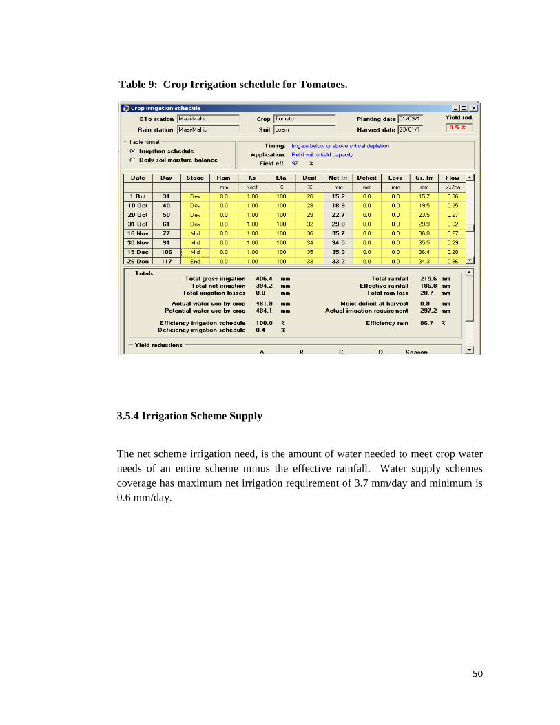
50
Table 9: Crop Irrigation schedule for Tomatoes.
3.5.4 Irrigation Scheme Supply
The net scheme irrigation need, is the amount of water needed to meet crop water
needs of an entire scheme minus the effective rainfall. Water supply schemes
coverage has maximum net irrigation requirement of 3.7 mm/day and minimum is
0.6 mm/day.
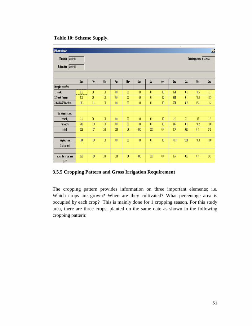
51
Table 10: Scheme Supply.
3.5.5 Cropping Pattern and Gross Irrigation Requirement
The cropping pattern provides information on three important elements; i.e.
Which crops are grown? When are they cultivated? What percentage area is
occupied by each crop? This is mainly done for 1 cropping season. For this study
area, there are three crops, planted on the same date as shown in the following
cropping pattern:
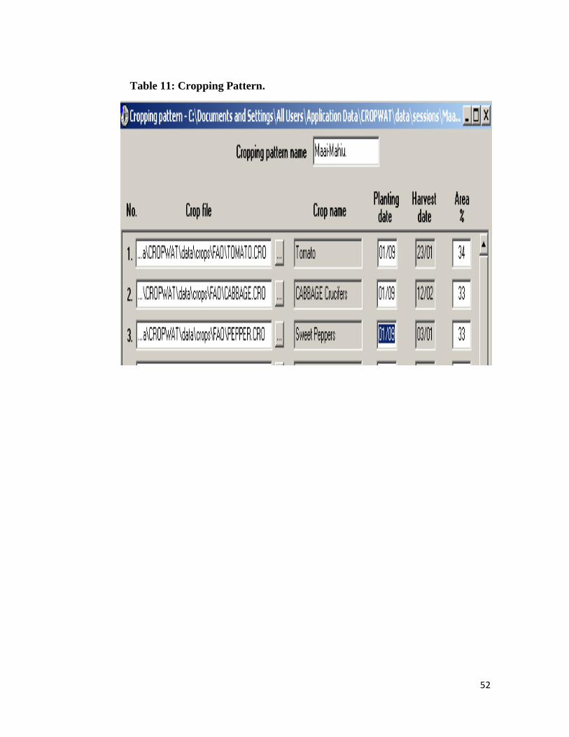
52
Table 11: Cropping Pattern.
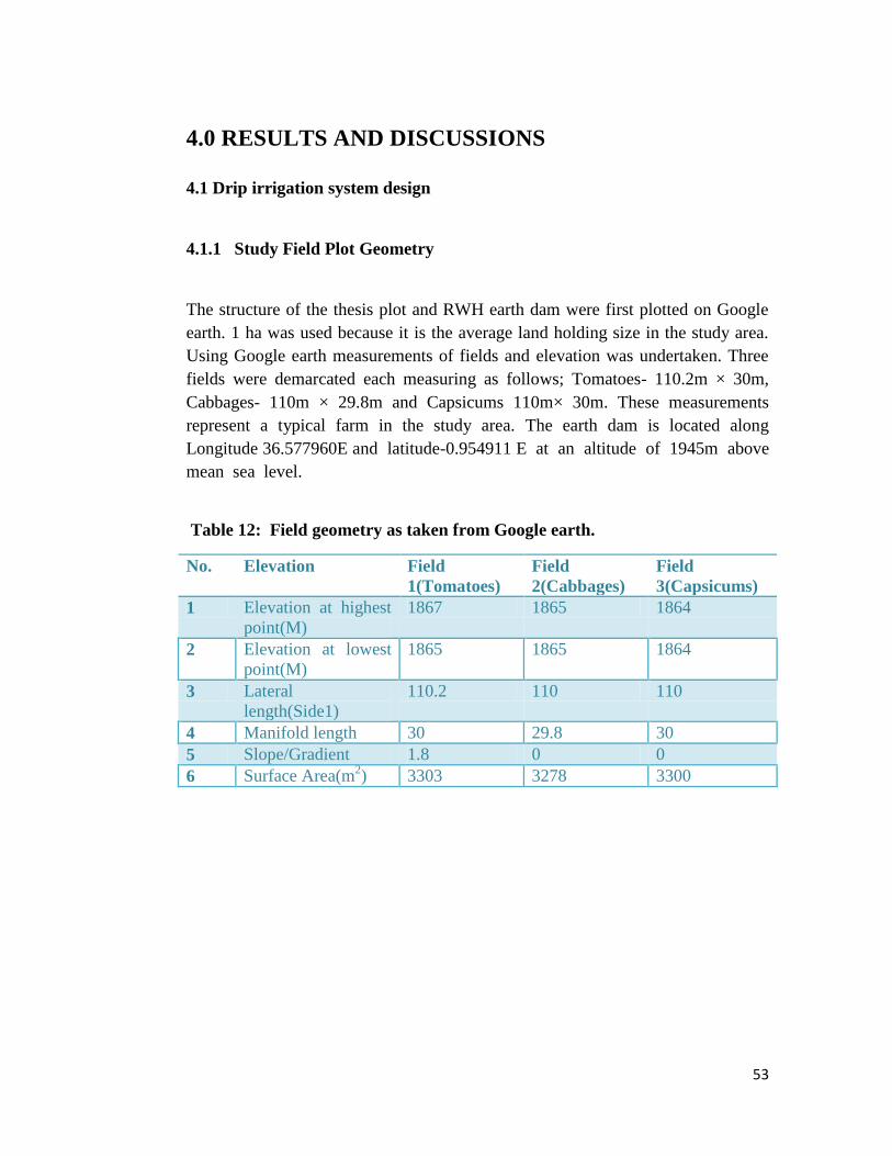
53
4.0 RESULTS AND DISCUSSIONS
4.1 Drip irrigation system design
4.1.1 Study Field Plot Geometry
The structure of the thesis plot and RWH earth dam were first plotted on Google
earth. 1 ha was used because it is the average land holding size in the study area.
Using Google earth measurements of fields and elevation was undertaken. Three
fields were demarcated each measuring as follows; Tomatoes- 110.2m × 30m,
Cabbages- 110m × 29.8m and Capsicums 110m× 30m. These measurements
represent a typical farm in the study area. The earth dam is located along
Longitude 36.577960E and latitude-0.954911 E at an altitude of 1945m above
mean sea level.
Table 12: Field geometry as taken from Google earth.
No. Elevation Field
1(Tomatoes)
Field
2(Cabbages)
Field
3(Capsicums)
1 Elevation at highest
point(M)
1867 1865 1864
2 Elevation at lowest
point(M)
1865 1865 1864
3 Lateral
length(Side1)
110.2 110 110
4 Manifold length 30 29.8 30
5 Slope/Gradient 1.8 0 0
6 Surface Area(m2) 3303 3278 3300
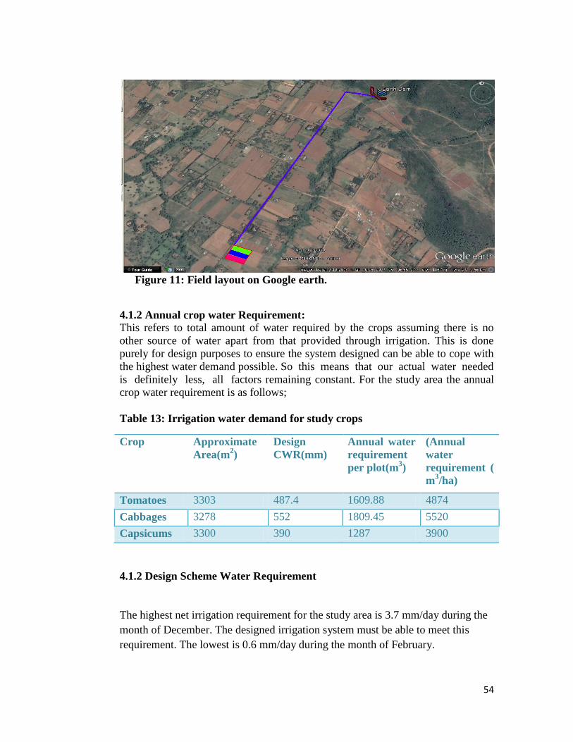
54
Figure 11: Field layout on Google earth.
4.1.2 Annual crop water Requirement:
This refers to total amount of water required by the crops assuming there is no
other source of water apart from that provided through irrigation. This is done
purely for design purposes to ensure the system designed can be able to cope with
the highest water demand possible. So this means that our actual water needed
is definitely less, all factors remaining constant. For the study area the annual
crop water requirement is as follows;
Table 13: Irrigation water demand for study crops
Crop Approximate
Area(m2)
Design
CWR(mm)
Annual water
requirement
per plot(m3)
(Annual
water
requirement (
m3/ha)
Tomatoes 3303 487.4 1609.88 4874
Cabbages 3278 552 1809.45 5520
Capsicums 3300 390 1287 3900
4.1.2 Design Scheme Water Requirement
The highest net irrigation requirement for the study area is 3.7 mm/day during the
month of December. The designed irrigation system must be able to meet this
requirement. The lowest is 0.6 mm/day during the month of February.
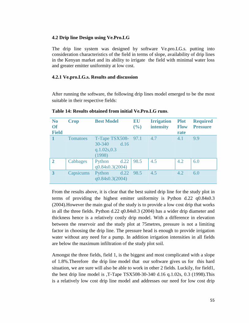
55
4.2 Drip line Design using Ve.Pro.LG
The drip line system was designed by software Ve.pro.LG.s. putting into
consideration characteristics of the field in terms of slope, availability of drip lines
in the Kenyan market and its ability to irrigate the field with minimal water loss
and greater emitter uniformity at low cost.
4.2.1 Ve.pro.LG.s. Results and discussion
After running the software, the following drip lines model emerged to be the most
suitable in their respective fields:
Table 14: Results obtained from initial Ve.Pro.LG runs.
No
Of
Field
Crop Best Model EU
(%)
Irrigation
intensity
Plot
Flow
rate
Required
Pressure
1 Tomatoes T-Tape TSX508-
30-340 d.16
q.1.02s,0.3
(1998)
97.1 4.7 4.1 9.9
2 Cabbages Python d.22
q0.84s0.3(2004)
98.5 4.5 4.2 6.0
3 Capsicums Python d.22
q0.84s0.3(2004)
98.5 4.5 4.2 6.0
From the results above, it is clear that the best suited drip line for the study plot in
terms of providing the highest emitter uniformity is Python d.22 q0.84s0.3
(2004).However the main goal of the study is to provide a low cost drip that works
in all the three fields. Python d.22 q0.84s0.3 (2004) has a wider drip diameter and
thickness hence is a relatively costly drip model. With a difference in elevation
between the reservoir and the study plot at 75metres, pressure is not a limiting
factor in choosing the drip line. The pressure head is enough to provide irrigation
water without any need for a pump. In addition irrigation intensities in all fields
are below the maximum infiltration of the study plot soil.
Amongst the three fields, field 1, is the biggest and most complicated with a slope
of 1.8%.Therefore the drip line model that our software gives us for this hard
situation, we are sure will also be able to work in other 2 fields. Luckily, for field1,
the best drip line model is ,T-Tape TSX508-30-340 d.16 q.1.02s, 0.3 (1998).This
is a relatively low cost drip line model and addresses our need for low cost drip
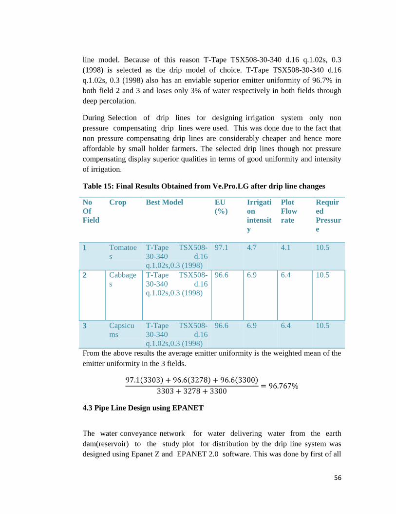
56
line model. Because of this reason T-Tape TSX508-30-340 d.16 q.1.02s, 0.3
(1998) is selected as the drip model of choice. T-Tape TSX508-30-340 d.16
q.1.02s, 0.3 (1998) also has an enviable superior emitter uniformity of 96.7% in
both field 2 and 3 and loses only 3% of water respectively in both fields through
deep percolation.
During Selection of drip lines for designing irrigation system only non
pressure compensating drip lines were used. This was done due to the fact that
non pressure compensating drip lines are considerably cheaper and hence more
affordable by small holder farmers. The selected drip lines though not pressure
compensating display superior qualities in terms of good uniformity and intensity
of irrigation.
Table 15: Final Results Obtained from Ve.Pro.LG after drip line changes
No
Of
Field
Crop Best Model EU
(%)
Irrigati
on
intensit
y
Plot
Flow
rate
Requir
ed
Pressur
e
1 Tomatoe
s
T-Tape TSX508-
30-340 d.16
q.1.02s,0.3 (1998)
97.1 4.7 4.1 10.5
2 Cabbage
s
T-Tape TSX508-
30-340 d.16
q.1.02s,0.3 (1998)
96.6 6.9 6.4 10.5
3 Capsicu
ms
T-Tape TSX508-
30-340 d.16
q.1.02s,0.3 (1998)
96.6 6.9 6.4 10.5
From the above results the average emitter uniformity is the weighted mean of the
emitter uniformity in the 3 fields.
4.3 Pipe Line Design using EPANET
The water conveyance network for water delivering water from the earth
dam(reservoir) to the study plot for distribution by the drip line system was
designed using Epanet Z and EPANET 2.0 software. This was done by first of all
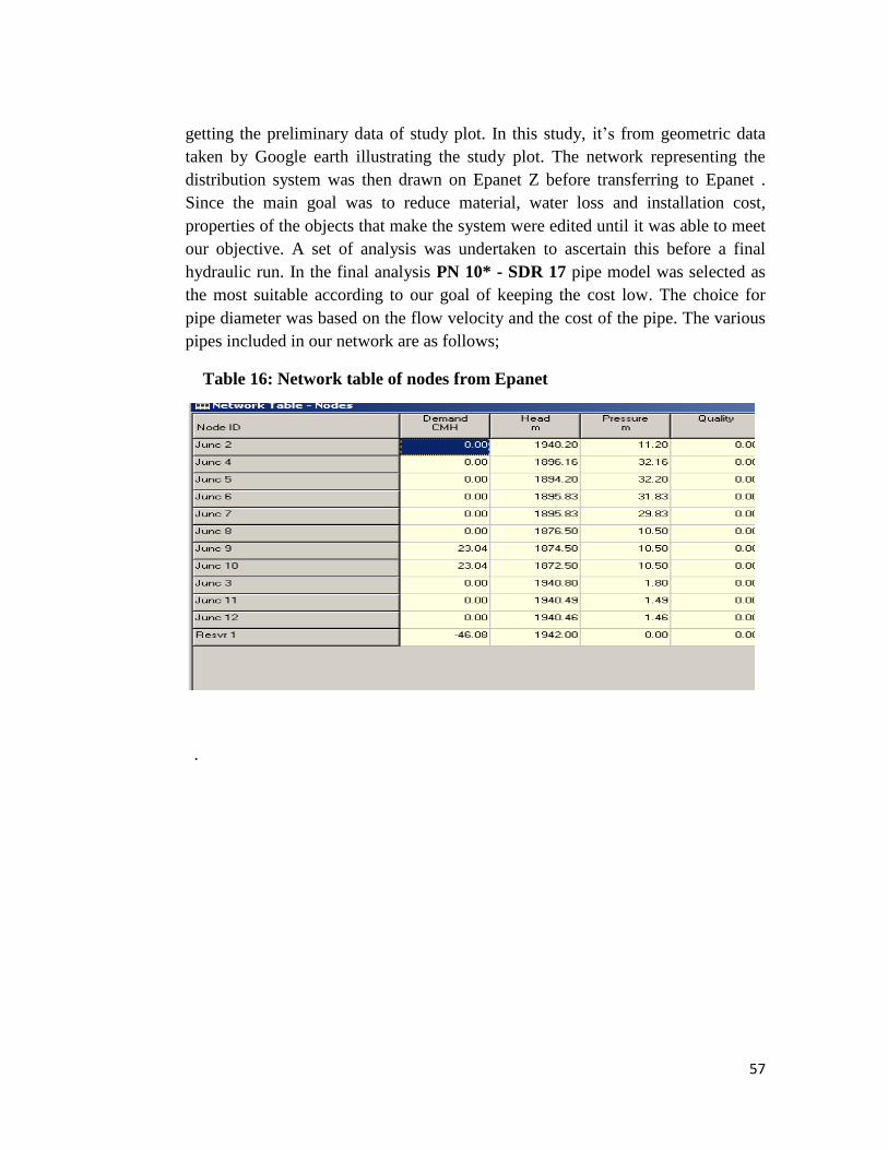
57
getting the preliminary data of study plot. In this study, it‘s from geometric data
taken by Google earth illustrating the study plot. The network representing the
distribution system was then drawn on Epanet Z before transferring to Epanet .
Since the main goal was to reduce material, water loss and installation cost,
properties of the objects that make the system were edited until it was able to meet
our objective. A set of analysis was undertaken to ascertain this before a final
hydraulic run. In the final analysis PN 10* - SDR 17 pipe model was selected as
the most suitable according to our goal of keeping the cost low. The choice for
pipe diameter was based on the flow velocity and the cost of the pipe. The various
pipes included in our network are as follows;
Table 16: Network table of nodes from Epanet
.
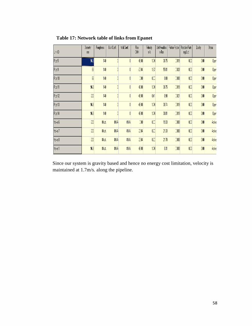
58
Table 17: Network table of links from Epanet
Since our system is gravity based and hence no energy cost limitation, velocity is
maintained at 1.7m/s. along the pipeline.
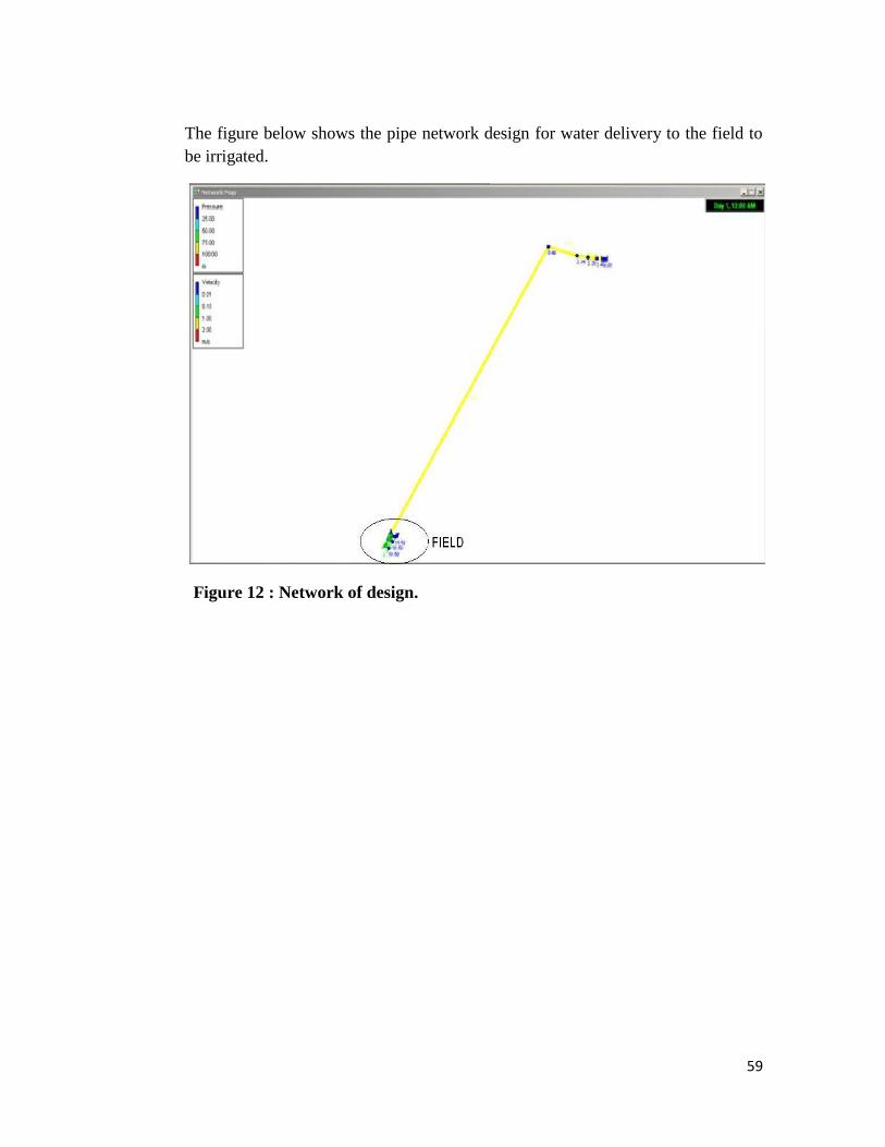
59
The figure below shows the pipe network design for water delivery to the field to
be irrigated.
Figure 12 : Network of design.
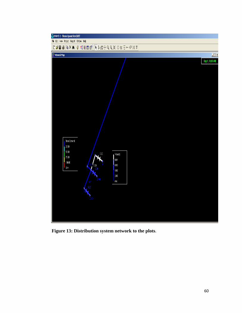
60
Figure 13: Distribution system network to the plots.
61
4.4 Discussion
4.4.1 Discussion of RWH Potential results.
The average annual runoff that can be collected from the study area is 188.4mm.
Using Google maps, the size of the catchment was calculated to be 4.3km2
.Therefore the amount of water that can possible be harvested from the catchment
assuming an efficiency level of 90% is 728,930m3 . This is a good indication that
farmers in Maai-Mahiu area in deed can be able to rely on RWH to grow crops
profitably. However to harvest all this water will require construction of a large
dam covering an area of 18.22ha. This may not be possible for individual small
scale farmers .Large dams with embankment wall measuring over 15m can only be
designed and constructed by qualified and registered engineer. These farmers
however can construct small earth dams by themselves manually and be able to
take advantage of this massive runoff.
With an average of irrigation requirement of 5000m3/ha, this harvested water is
enough to irrigate 145.786ha of land. If each farmer has on average 1ha of land,
this will be enough to support 145 farmers with sufficient water for irrigation. The
annual average rainfall received in the study area is 795mm. Therefore a runoff of
188.4mm comprises 24% of this average annual rainfall.
4.4.2 Discussion of irrigation system design results:
The study plot has irrigation intensity like 6.9 mm/hour and a peak gross irrigation
of 3.82 mm per day. Therefore it is possible to irrigate all the three plots in the
field in 1.5hours.To better exploit our pipes and give water for all farms in an
efficient and organised manner, the main pipe is designed to carry double our flow
rates. Therefore in a 24 hour period, If 2 farms are irrigated together 32 similar
farms in the locality can be irrigated. This information is very important because it
can help in irrigation scheduling. With our main conveyance pipeline measuring
1432metres in length its possible to irrigate 16 similar fields on both side of the
main conveyance pipe each having a similar manifold length of about 90m. With
this information when the scheme is developed it would be easy to plan an
irrigation schedule and better utilization of the earth dam.
In the design though pressure is not a limiting factor because the system relies on
gravity, care has been taken to avoid using bigger size pipes. This is because
62
bigger pipes cost more and will go against our goal of designing low cost irrigation
system. No provision was given for minor loses because our head is not a limiting
factor.
Since the pressure from reservoir is quite high, pressure reducing valve (PRV) was
included on the design system to control pressure head at the fields in take point.
The valve is also a safe guard to control pressure to the required operating level
whenever necessary.
One of the main problems with drip irrigation is blockage of the emitters. Emitters
have very small waterways that are below 2.0 mm in diameter and can easily block
if the water is not clean. Thus it is essential for irrigation water to be free of
sediments. To ensure that this is achieved a filter has been installed within our
Epanet design.
63
5.0 CONCLUSION AND RECOMMENDATIONS
5.1 Conclusion
Modeling using custom made irrigation software provide an easy way of designing
of irrigation systems. This way the designer is able to target the three most
important goals of irrigation system design. These goals include reduction of
material and installation cost; reduction of energy cost and finally reduction of
water loss. By adopting use of irrigation software, a designer is able to model a
system that meets the aforementioned goals all at the same time with a lot of ease.
Rainwater harvesting provide a greater possibility for improving agriculture
production. It is an efficient and sustainable way to improve crop production most
especially in ASAL areas. RWH is one option to use runoff better by capturing
and storing when rainfall is abundant for use in periods when there is scarcity. As
has been seen in this study selection of suitable areas for RHW requires proper
understanding of a number of critical factors key among them soil, climate,
topography and land use.
This study attempted to pursue the possibility of harnessing rainwater for crop
production in Maai-Mahiu. In order to address technical short comings in design,
runoff curve numbers was adopted to determine the optimal design parameters.
This procedure takes into account all the input parameters. This included daily
rainfall figures for the study area for 13 years, soil type, and land use
classification. In this study, use of Runoff curve numbers proved to be a suitable
tool for analyzing areas suitable for RWH interventions and estimating amount of
runoff that can be harvested in an area.
The major outcome of this study is the fact that Maai-Mahiu as are other similar
ASAL areas in Kenya has got huge RWH potential. This potential if well
harnessed is able to transform these dry regions to become food baskets. A
catchment of 4.3km2, for example from the analysis can be able to harvest
728,930m3
of water. This can able to provide enough water to irrigate 145 ha of
land excluding rainfall input. If for example rainfall is included and harvested
water used only to supplement rain much more land can be put under production.
Efficient use of water is seen as a key to crop production in ASAL areas in sub
Sahara Africa. This is increasingly true because of ever –increasing populations
and demand for food production coupled with growing competition for water and
increasing energy costs. For small holder farmers, drip irrigation provides means
64
of maximizing returns on their crop land by increasing the economic biomass
production per unit of water. It provides good water control by delivering water
near the plant; enabling the farmer to grow crops with much less water compared
to other irrigation methods.
In this study, a low Cost drip irrigation system has been successfully designed for
the local situation with an impressive efficiency of 96.7%. Because of the
topography of the area, farmers can save themselves a lot of money by leveraging
on gravity for water conveyance from the reservoir without need for pumps.
Farmers can harvest the water from upland areas and convey it by gravity to
their fields located downstream. This will also go a long way in making their
production profitable because gravity fed irrigation is cheaper in comparison to
pump fed irrigation.
5.2 Recommendations
The future of agriculture in ASAL areas lies majorly on how water harvesting and
storage infrastructure can be developed. This is where government should direct
resources as it directly addresses food insecurity and high poverty levels. Irrigation
improves people‘s welfare through improved and stable crop yields and incomes.
This also goes a long way in curbing rural to urban migration and hence social
unrests in urban areas.
The cost of establishing RWH structures and drip irrigation system is quite
enormous to be met by a majority of small holder farmers. This proposal can be
forwarded to various governmental agencies such as CDF, County government or
NIB not forgetting donors and multi lateral financing agencies for funding
consideration. It is important to ensure from the beginning that the users of
irrigation water are involved in irrigation system design. It is important for
designer to incorporate the wishes of users regarding agronomic, economic and
organisational aspects. Past evidence show that schemes where users are not
involved when designing performed below par and never achieve their objectives.
In the mean time small dams and ponds can be built easily by self-help groups.
Group members encourage each other and have higher implementation capacity as
they easily tap idle labour. Farmers can organise themselves in groups and develop
smaller dams in the catchment area. In the short term farmers can also rely on
cheap second hand drip irrigation equipment which is sold at lower prices by large
horticultural farms in the nearby Naivasha area.
65
To ensure success and sustainability, it is imperative that farmers are educated on
practical use of irrigation systems not forgetting agronomic practices. There is also
need to train them on the need for proper maintenance, especially periodic
desilting of dams and replacement of worn out equipments and materials. In
addition due to climate variability farmers should be sensitised on the utilization of
drought-tolerant crop varieties and rearing of drought –adapted livestock breeds.
To enjoy benefits of economies of scale, farmers need to organise themselves in a
cooperative society. This will help bring them together with a common interest of
pulling resources together in order to carry out joint activities that are of mutual
benefit. This way they can be able to negotiate better terms in contract farming and
lower prices for agricultural inputs like seeds, fertilizer and equipment. In addition,
cooperatives offer prospects that smallholder farmers would not be able to achieve
individually such as helping them to secure cheaper bank loans and better market
opportunities. It is also easy for small holder farmers organised in a cooperative to
go into value addition and agro-processing and therefore make better returns from
their farm investments.
Using RWH irrigation systems to grow crops is potentially profitable in the study
area of Maai-Mahiu. This is mainly due to the fact that farmers can rely on gravity
unlike in other areas where water has to be pumped. However a true picture can
only be realized by conducting a cost benefit analysis of RWH in the area. A
further research should also be undertaken to establish actual crop water
requirements of the different crops grown under local climatic conditions. This
would go a long way in improving irrigation water management and hence water
productivity.
66
REFERENCES
Barron J, Okwach G (2005) Run-off water harvesting for dry spell mitigation in
maize (Zea mays L.): results from on-farm research in semi-arid Kenya.
Agricultural Water Management74,
FAO Irrigation and drainage Paper 33.
FAO irrigation and drainage paper No. 64- Manual on small earth dams -A guide
to siting, design and construction
Hatibu N, Mahoo H (1999) Rainwater harvesting technologies for agricultural
production: A case for Dodoma, Tanzania. Sokoine University of Agriculture
Department of Agricultural Engineering and Land Planning, Morogoro, Tanzania.
Hatibu N, Senkondo EM, Mutabazi K, Msangi ASK (2004) Economics of
Rainwater Harvesting for Crop Enterprises in Semi-Arid Areas. In 'New directions
for a diverse planet: Proceedings of the 4th International Crop Science Congress'.
Brisbane, Australia.
Heyer. J., Maitha, J.K., Senga, W.M., (1976).Achievements, problems and
prospects in the agricultural development in Kenya: An economic assessment, ed.
Nairobi; Oxford University press.
http://en.wikipedia.org/wiki/Runoff_curve_number
Irrigation methods: Drip irrigation—Options for smallholders by: Seleshi Bekele
Awulachew (IWMI), Philippe Lemperiere (IWMI) and Taffa Tulu (Adama
University), January 2009
Infonet –biovision; crops/fruits/vegetables., http://www.infonet-biovision.org
accessed on 20th
May 2014
J. W. Kaluli, K. Ng‘ang‘a, P. G.Home1, J. M. Athena, A.W. Muriuki and A.
W.Kihurani1- Research paper on the effect of rain water harvesting and drip
irrigation on crop performance in an arid and semi-arid environment
Manual on small earth dams-A guide to siting, design and construction (FAO
irrigation and drainage paper 64)
Mbatia, E. D., (2006).Irrigation sector in Kenya- status and challenges: ―Paper
presented during the ―green water credits workshop‖ Kari hq Nairobi.
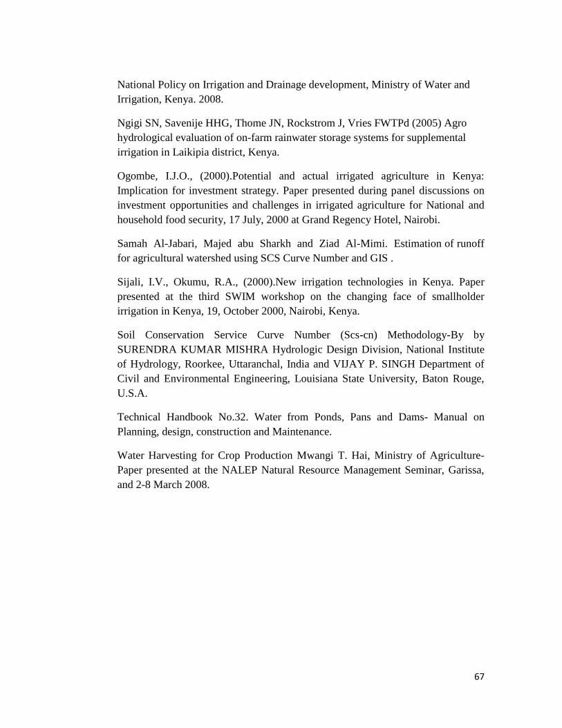
67
National Policy on Irrigation and Drainage development, Ministry of Water and
Irrigation, Kenya. 2008.
Ngigi SN, Savenije HHG, Thome JN, Rockstrom J, Vries FWTPd (2005) Agro
hydrological evaluation of on-farm rainwater storage systems for supplemental
irrigation in Laikipia district, Kenya.
Ogombe, I.J.O., (2000).Potential and actual irrigated agriculture in Kenya:
Implication for investment strategy. Paper presented during panel discussions on
investment opportunities and challenges in irrigated agriculture for National and
household food security, 17 July, 2000 at Grand Regency Hotel, Nairobi.
Samah Al-Jabari, Majed abu Sharkh and Ziad Al-Mimi. Estimation of runoff
for agricultural watershed using SCS Curve Number and GIS .
Sijali, I.V., Okumu, R.A., (2000).New irrigation technologies in Kenya. Paper
presented at the third SWIM workshop on the changing face of smallholder
irrigation in Kenya, 19, October 2000, Nairobi, Kenya.
Soil Conservation Service Curve Number (Scs-cn) Methodology-By by
SURENDRA KUMAR MISHRA Hydrologic Design Division, National Institute
of Hydrology, Roorkee, Uttaranchal, India and VIJAY P. SINGH Department of
Civil and Environmental Engineering, Louisiana State University, Baton Rouge,
U.S.A.
Technical Handbook No.32. Water from Ponds, Pans and Dams- Manual on
Planning, design, construction and Maintenance.
Water Harvesting for Crop Production Mwangi T. Hai, Ministry of Agriculture-
Paper presented at the NALEP Natural Resource Management Seminar, Garissa,
and 2-8 March 2008.
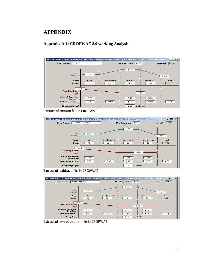
68
APPENDIX
Appendix A 1: CROPWAT 8.0 working Analysis
Extract of tomato file in CROPWAT
Extract of cabbage file in CROPWAT
Extract of sweet pepper file in CROPWAT
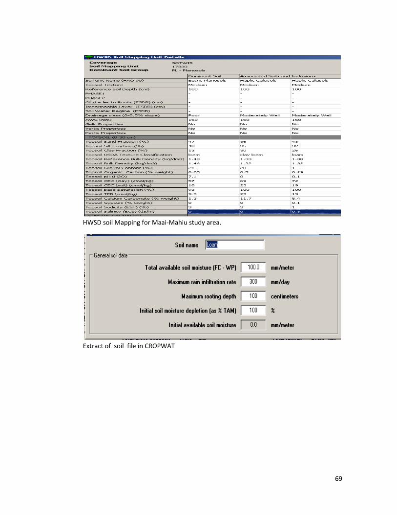
69
HWSD soil Mapping for Maai-Mahiu study area.
Extract of soil file in CROPWAT
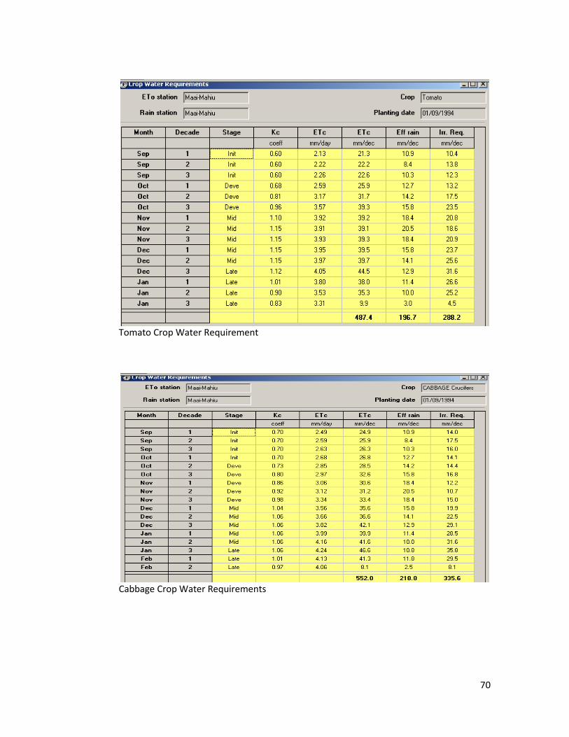
70
Tomato Crop Water Requirement
Cabbage Crop Water Requirements
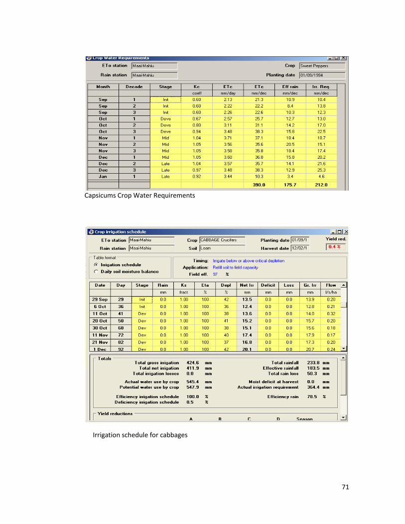
71
Capsicums Crop Water Requirements
Irrigation schedule for cabbages
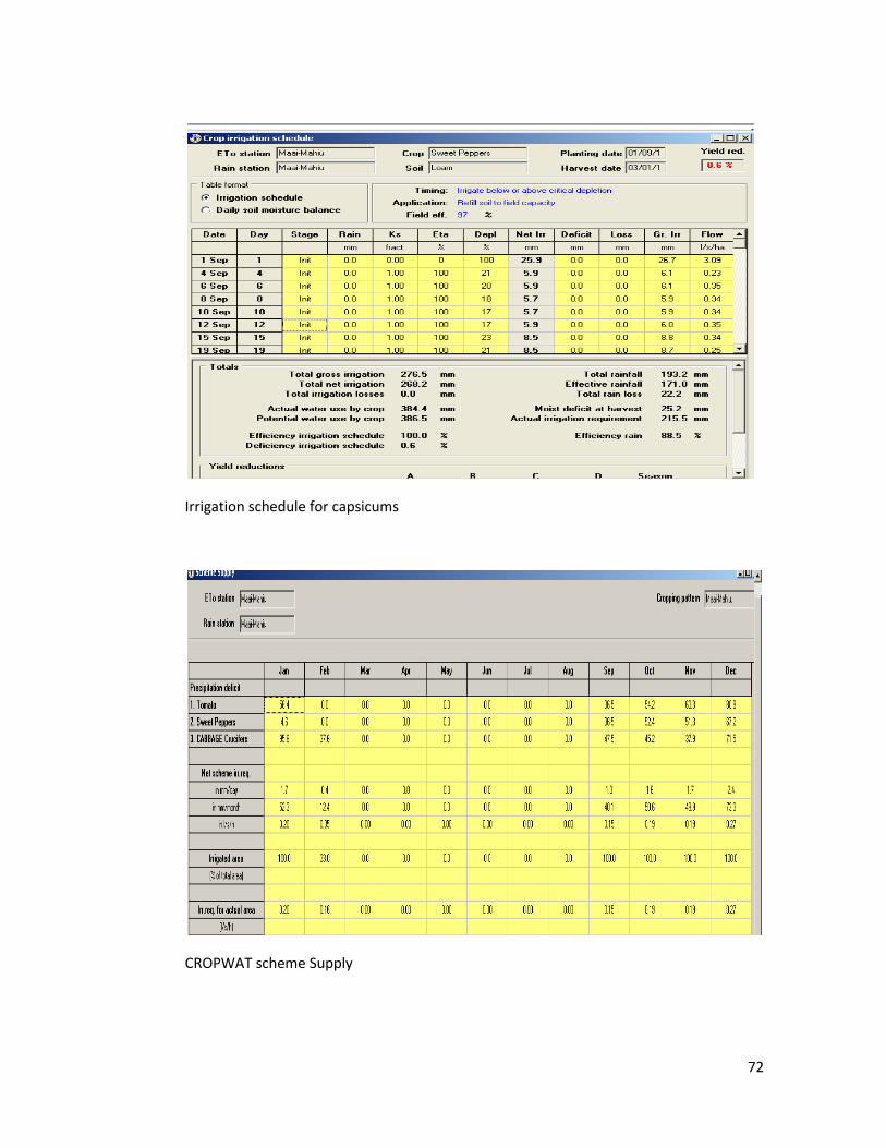
72
Irrigation schedule for capsicums
CROPWAT scheme Supply
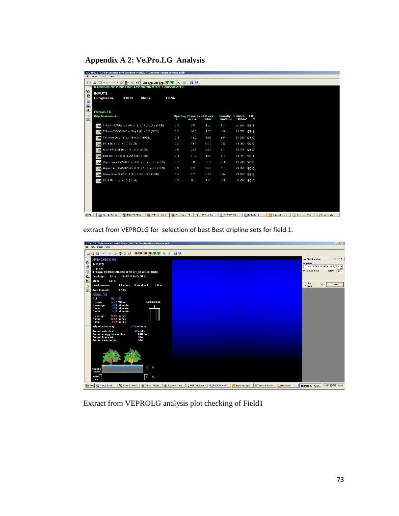
73
Appendix A 2: Ve.Pro.LG Analysis
extract from VEPROLG for selection of best Best dripline sets for field 1.
Extract from VEPROLG analysis plot checking of Field1
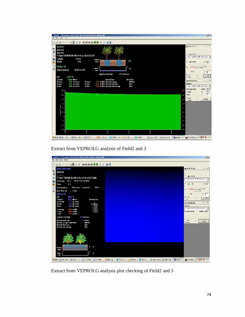
74
Extract from VEPROLG analysis of Field2 and 3
Extract from VEPROLG analysis plot checking of Field2 and 3
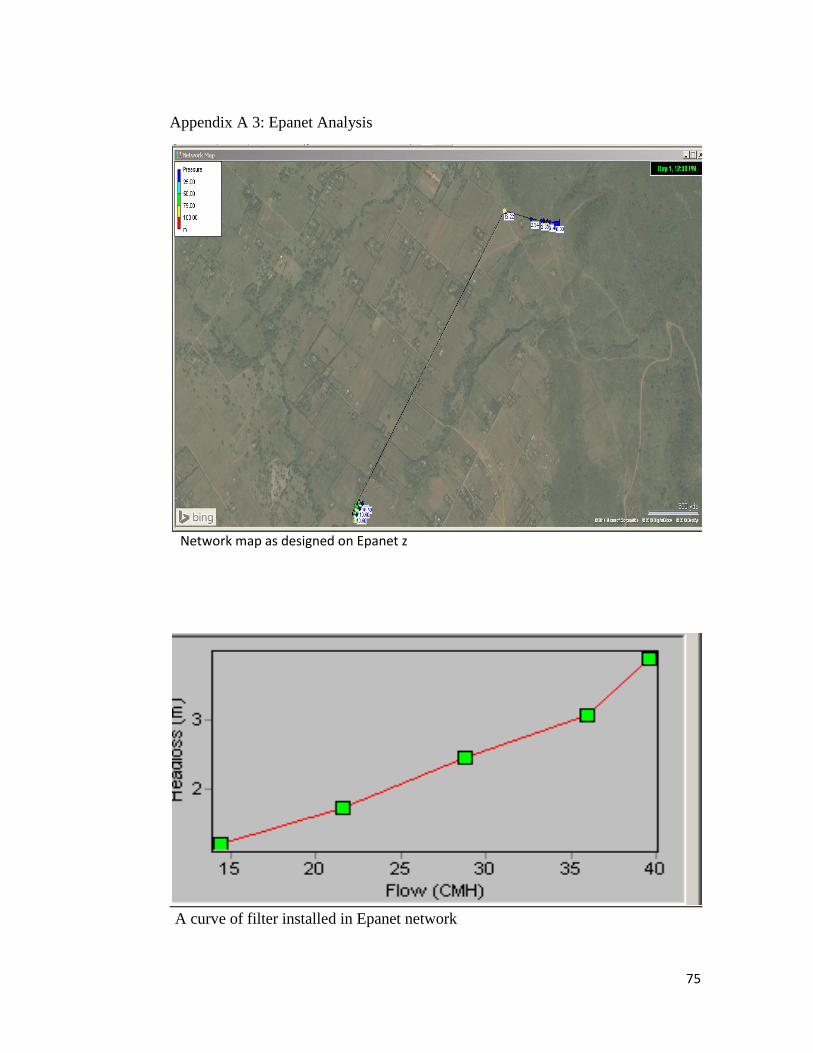
75
Appendix A 3: Epanet Analysis
Network map as designed on Epanet z
A curve of filter installed in Epanet network
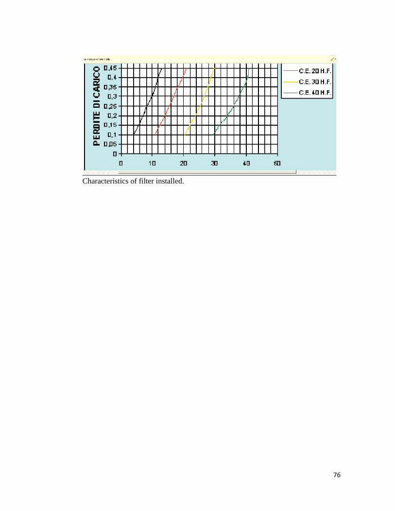
76
Characteristics of filter installed.
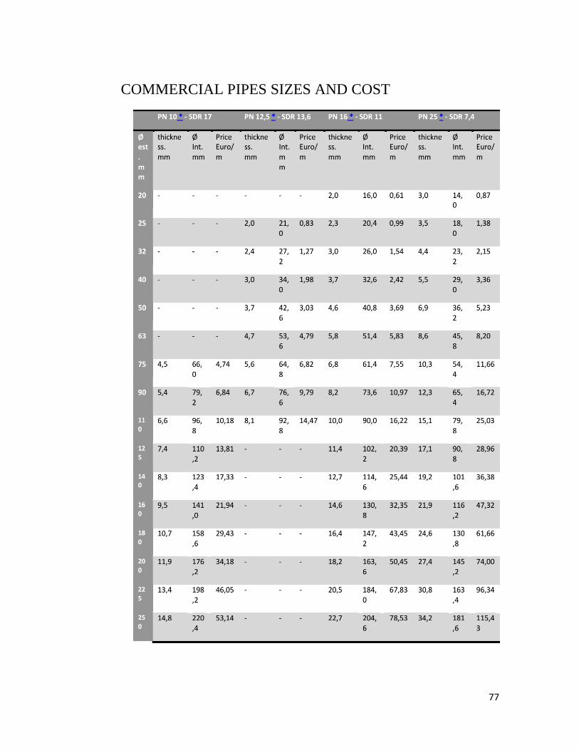
77
COMMERCIAL PIPES SIZES AND COST
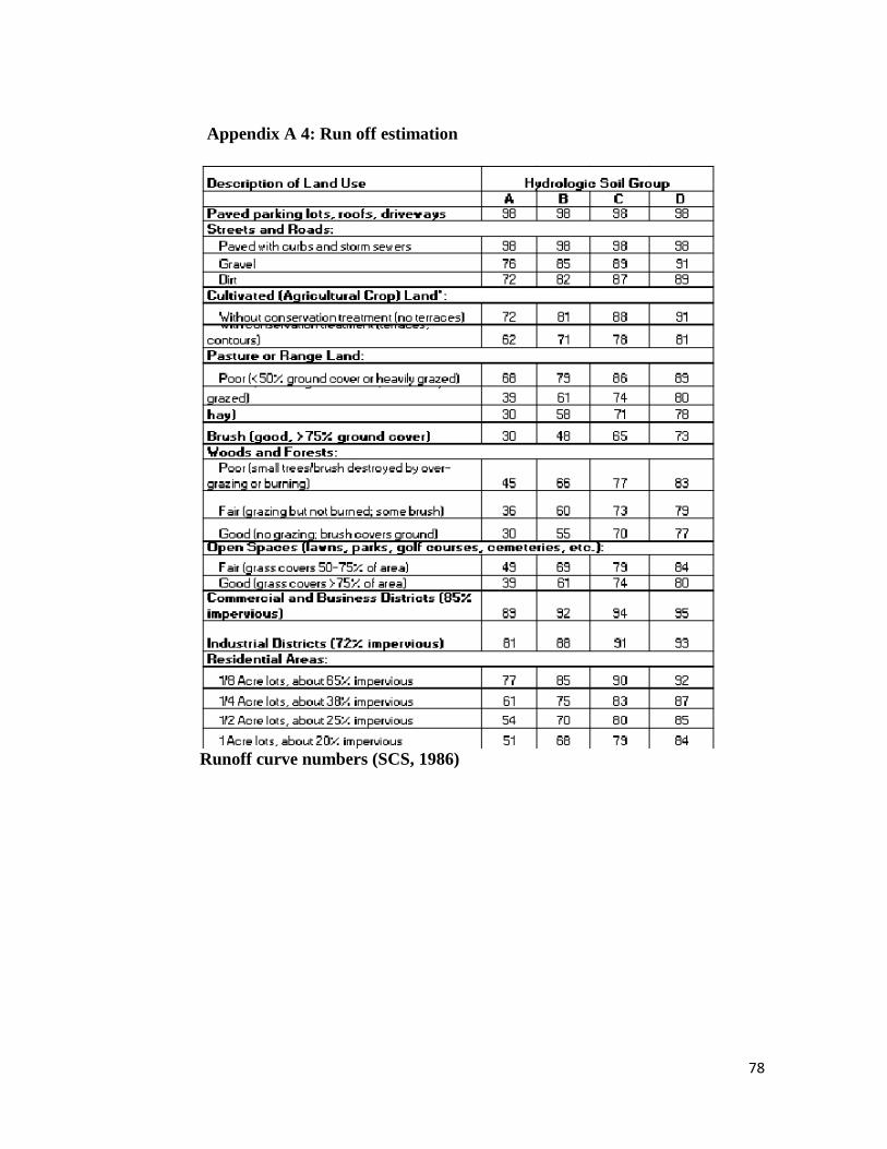
78
Appendix A 4: Run off estimation
Runoff curve numbers (SCS, 1986)