usrp project final report

EECS 399 Project

Understanding a Basic OFDM Transceiver with

GNU Radio and USRPs

Arjan Gupta

(Under the guidance of Dr. Aveek Dutta)

Understanding a Basic OFDM Transceiver with GNU Radio and USRPs Page 1

Contents

Section 1 – Project Objective

Background and Introduction ………………………………………………………. Page 3

Learning Potential and Takeaways of this Project ……………….…………....…… Page 3

Why this Knowledge is Important ……….……….………………..…….….……… Page 3

Real System Implementation ……………………………………..……...……….… Page 4

Section 2 – Technical Concepts/Details Understood Through this Project

Basic Digital Signal Processing (DSP) ………………….………………………….. Page 4

Nyquist-Shannon Sampling Theorem

Analog-to-Digital Convertor

Signal Reconstruction

Other DSP operations

IEEE 802.11 PPDU Frame Formats …………………………………..…….……… Page 7

PLCP Preamble Construction Using MATLAB

Signal-to-Noise Ratio ……………………………………..………..…….……….... Page 9

Friis Transmission Equation

Path Loss (in Media and at High Frequencies)

Interference and Diffraction of EMW

Noise Temperature

Software Defined Radio ………………………………………….…...………...… Page 11

Section 3 – The Experimental Setup

Universal Software Defined Radio Peripheral (USRP) …………….…….…..…… Page 11

GNU Radio ……………………………………………………...……….………... Page 12

Bastian Bloessl’s OFDM Transceiver ………………………………….…………. Page 14

Overall Setup Block Diagram …….…..…..……………………..…….………….. Page 14

Pictures of the Actual Setup ………………………………………….…...………. Page 15

Section 4 – Performing the Experiment and Results

Performing the Experiment ………………………………………………..……… Page 17


Initial Simulation

Getting at the Actual Transceiver to Work

Transmitter and Receiver Signal Plots

Results Obtained ……………………………………………………………………. Page 22

Observed SNR Variation in the Line of Sight with Distance

Observed SNR Variation for Path Loss

More Analysis of Results ……………….……………………………….………..... Page 23

Section 5 – Possible Future Work

Programming the FPGA of the USRP………………………………..…………....... Page 24

EECS Senior Thesis

Section 6 – Code Appendix

Signal Reconstruction Code ……………………………………………………….. Page 24

PLCP Preamble Construction Code ………………………………………….……. Page 25

TX Captured Signal Plot Code …………………………………………………….. Page 26

RX Captured Signal Plot Code …………………………………………………….. Page 26

FER vs. Distance Plot Code ………………………………………………………... Page 27

Section 7 – Bibliography

Works Referenced …...……………………………...…………………………….... Page 28


Project Objective

Background and Introduction

Our interest in this area of research has its background in an introductory level course taught within the

Electrical Engineering and Computer Science (EECS) Department at the University of Kansas, called

Introduction to Communication Networks (EECS 563). This course covers a discussion of the uses of

communication networks, network protocols, standards, and traffic (all discussed in a layered reference

model). The key take-away from EECS 563 that inspired this independent study is how packet information

communication takes place in the wireless domain. We became interested with how transceivers work

with the 802.11 standard and decided to dive into a full-fledged study of a simple OFDM (Orthogonal

Frequency Division Multiplexing) transceiver using GNU Radio Software and Universal Software

Defined Radio Peripherals (USRPs).

Learning Potential and Takeaways of this Project

This field of study focused on a vast area of electrical engineering and computer science, which has an

infinite learning potential. Therefore, lot can be learned (and was so learned) from this project. The way

we have set up this project also affects what we take away from the project. We would do this project on

a Raspberry Pi computer with relatively simple computing, where a software such as GNU Radio would

not be able to run in its optimal potential. Such a project would give us a good learning experience not

just about OFDM transceiver in IEEE standard 802.11, but also an embedded systems approach toward

it.

However, we implemented our project on a standard computing running the Linux Ubuntu 14.04 operating

system, on top of which we ran the GNU Radio software, which lets us design and implement simple

receiver/transmitter blocks using a GUI or by manually writing code in Python. We also used a Universal

Hardware Device (UHD) called the Universal Software Defined Radio Peripheral (USRP), which has its

own source code written in C++, but GNU Radio can easily interact with a USRP because of the way this

software system is developed.

Hence, this project teaches us the following: a great deal about IEEE 802.11 OFDM standards for packet-

based data communication, a practical understanding of digital signal processing, an introduction to

software defined radio, a great deal of experience with using the Linux environment and shell scripting,

and application based experience with programming in Python, C++, and MATLAB.

Why this Knowledge is Important

The student researcher of this project, Arjan Gupta, is a junior pursuing a Computer Engineering major.

The takeaways of this independent study cover a good amount of both hardware and software, which not

only touches upon the essence of computer engineering in general with the field of, but are also in the

personal academic interest of the student researcher. This independent study will help the student

researcher achieve his endeavor of developing this study into thesis-oriented research project in his senior

year.

The learnings of this project are quite generally useful as well. A good understanding of an OFDM

transceiver will give the researcher learning outcomes that are applicable in industry-based jobs or


graduate school level research endeavors. This is because nowadays, basic academic coursework is not

enough to learn a concept. Practical experience is a necessity, which is exactly what this project gives us.

Also, transceivers and communication systems (software based or not) are present everywhere around us.

Many electronics applications today can inter-mingle with communication systems. Therefore, any

knowledge in this division of electrical engineering and computer science world is undoubtedly important

and useful.

Real-System Implementation

It is important to note throughout this project that we are creating quite a simple and uncomplicated model

of a transceiver, which does not have a direct application in the real world. We are going to perform

experiments, and simulations, which, although practical, are to just give us a simplified understanding of

how data transmission and reception works in actual application based scenarios.

Even in the simplified transceiver we are going to create in this project, we will first simulate the model

and then actually carry out data transmission and reception. However, we will find that simulations are

ideal and in reality the experiment will have a number of aberrations. Most of the aberrations occur on the

receiver side because of signal distortion due to noise and other factors. Before understanding these factors

we must understand some key concepts, which are outlined in the following section.

Technical Concepts/Details Understood Through this Project

Basic Digital Signal Processing (DSP)

Our background from Signal and System Analysis class (EECS 360) will come in use here.

Nyquist-Shannon Sampling Theorem

For any band-limited signal, the Nyquist-Shannon Sampling Theorem (a.k.a. Sampling Theorem) tells us

that the signal must be sampled at the rate (fS) of at least two times the value of the band frequency (fB).

In other words,

𝑓𝑆 ≥ 2𝑓𝐵

This is how we will avoid something called ‘aliasing’ in our transceiver model, which happens when the

ends of two samples of the signal overlap each other. When aliasing happens, the sections of the samples

that overlapped appear to be missing from the signal when the signal is completely reconstructed. The

least frequency at which we can sample the incoming analog signal is called the Nyquist frequency. It is

important for us to operate our receiver at the Nyquist rate because we do not want aliasing in our signal.

Analog-to-Digital Convertor

An analog-to-digital convertor (ADC) is a device that converts a continuous physical quantity to a

discrete physical quantity (or digital quantity). We consider an amplitude versus time waveform that is


input to an ADC in the figure below.

In Figure 1, the working of an ADC is shown. The first part (Stage 1) is where a Sampling and Holding

circuit (S/H) samples the signal at a value that is at least the Nyquist rate for the input signal. Once the

signal is sampled, it is passed into the Quantizer, which is Stage 2 of the ADC. Here, each sample of the

signal is given an encoded binary number label according to its amplitude. This encoded binary numbers

are chosen from a limited number of possible values. In Figure 1, the numbers corresponding to the signal

samples are numbers in modulo 10, but these can easily be assigned their corresponding binary number

equivalents.

Signal Reconstruction

Once our signal is received after being transmitted through the air or a transmission channel (e.g. co-axial

cable), we might want to use the chunks of signal (the samples) to reconstruct the original signal. Without

this we cannot properly gain the information being transmitted in the signal.

Figure 1: ADC diagram [1]

Figure 2: Reconstruction block diagram [2]


Consider the block diagram in Figure 2 above. In this diagram, a reconstruction of signal is taking place

from a given analog signal. For example, if the signal in A is a continuous cosine function, then the signal

is first sampled so that it can be transmitted easily. After that, the sampled signal can be digitally

transmitted. Then the signal is reconstructed and plotted. The output signal looks closer and closer to the

input signal with higher values of the sampling interval. In fact, using MATLAB code, we generated the

plots in Figure 3, so that we can actually confirm this.

In Figure 3, we have sampled a cosine function given as cos(20πt) (which has a Nyquist frequency of 20

Hz) at four different sampling interval (T), which are 0.001 seconds (for first sub-plot), 0.01 seconds (for

second sub-plot), 0.05 seconds (for third sub-plot), and 0.1 seconds (for fourth sub-plot). This means that

the sampling frequencies in the three cases (f = 1/T), are 1000 Hz, 100 Hz, 20 Hz, and 10 Hz. This is why

in the third sub-plot we can see just a straight line, because aliasing of the rectangular pulses occurred

while sampling. This is because 10 Hz is lower than the Nyquist rate. Otherwise, at and above the Nyquist

rate, the signal is reconstructed better and better. The code for this reconstruction is given in the Code

Appendix.

Other DSP operations

There are other Digital Signal Processing operations that for which brief understanding was developed.

A multiply-accumulate operation (performed by a multiply-accumulator a.k.a. MAC), is involved in

reconstruction of the signal. A moving average filter operation smoothens out the waveform to correct

Figure 3: Reconstructing a cosine signal with rectangular pulses.


aberrations. Also, automatic gain control (AGC) is a closed-loop feedback regulating circuit, which

regulates the amplitude of the signal at its output, regardless of the amplitude of the signal at its input.

AGC is useful in adjusting the power of the signal at the receiver.

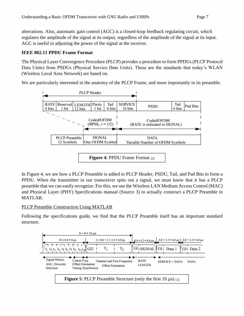
IEEE 802.11 PPDU Frame Format

The Physical Layer Convergence Procedure (PLCP) provides a procedure to form PPDUs (PLCP Protocol

Data Units) from PSDUs (Physical Service Data Units). These are the standards that today’s WLAN

(Wireless Local Area Network) are based on.

We are particularly interested in the anatomy of the PLCP Frame, and more importantly in its preamble.

In Figure 4, we see how a PLCP Preamble is added to PLCP Header, PSDU, Tail, and Pad Bits to form a

PPDU. When the transmitter in our transceiver spits out a signal, we must know that it has a PLCP

preamble that we can easily recognize. For this, we use the Wireless LAN Medium Access Control (MAC)

and Physical Layer (PHY) Specifications manual (Source 3) to actually construct a PLCP Preamble in

MATLAB.

PLCP Preamble Construction Using MATLAB

Following the specifications guide, we find that the PLCP Preamble itself has an important standard

structure.

Figure 4: PPDU Frame Format [3]

Figure 5: PLCP Preamble Structure (only the first 16 µs) [3]


In Figure 5 shown above, we see that the 16 µs PLCP Header is itself made up of two 8 µs sections. These

are the short and long parts of the preamble. The short part of the preamble is made up of ten short training

symbols (t1, t2, t3 … and so on up till t10). Each short training symbol is made up of 12 subcarriers, which

are given as the set S-26, 26 below:

Where the √13 6⁄ factor normalizes the power of the OFDM symbol. Then, an inverse Fast Fourier

Transform (IFFT) must be performed on the set, the set must be extended one and a half times, and the

set must go through a window function. The output of these steps construct the short part of the PLCP

preamble, as we need.

Now, the long part of the preamble has three parts, two of which are the long training symbols which are

quite long, so is not shown here, but can be found in the Wireless LAN Medium Access Control (MAC)

and Physical Layer (PHY) Specifications manual. After constructing a set, first we cut the long training

symbol in half, and put the second half behind the first. After that, similar to how we constructed the short

part of the preamble, we perform an IFFT, the set is extended and inputted to a window function. Once

we have the short and long parts of the PLCP preamble, we simple concatenate them to produce a full

PLCP preamble and then we plot its magnitude (the preamble will have complex values) it to get the

following figure:

Figure 6: Constructed PLCP Preamble


In Figure 5, we can we that there are two parts of the preamble, the first part being the short part of the

preamble and the second part being the long part of the preamble. Just as we would expect, both the

short and long parts of the preamble have a repetitive pattern, which is what helps us identify the

beginning of a PPDU packet.

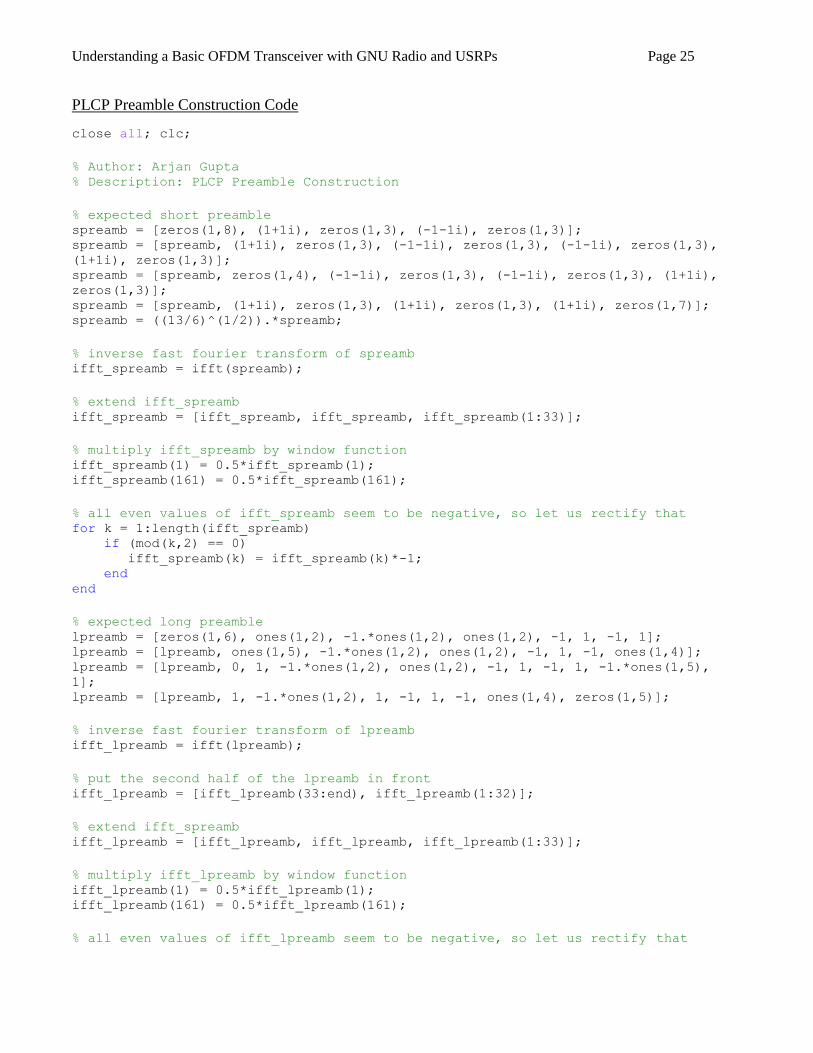
The actual MATLAB code we wrote to construct this preamble is given in the Code Appendix of this

report.

Signal-to-Noise Ratio (SNR)

Up till now we have illustrated concepts that were necessary in order to understand the basic working of

our transceiver. Now we come to a concept that will help us understand the aberrations that may be caused

in our data transmission, hence giving us non-ideal data at the receiver.

Signal-to-Noise Ratio (SNR), as the name suggests, is the ratio of the signal to the noise. It is given as:

𝑆𝑁𝑅 = 𝐴𝑣𝑒𝑟𝑎𝑔𝑒 𝑝𝑜𝑤𝑒𝑟 𝑜𝑓 𝑠𝑖𝑔𝑛𝑎𝑙

𝐴𝑣𝑒𝑟𝑎𝑔𝑒 𝑝𝑜𝑤𝑒𝑟 𝑜𝑓 𝑛𝑜𝑖𝑠𝑒

We desire lower noise, so in a general way, the higher the SNR it is, the more ideal it is for us.

There are many things that affect SNR, let us take a look at them.

Friis Transmission Equation

The Friis transmission equation establishes a relationship between the power of the signal at the receiving

antenna and the power of the signal at the transmitting antenna. The basic form of the equation is given

as:

Where, Pr and Pt are the power of the signal at the receiving and transmitting antennae respectively, the

Gt and Gt are the gain of the transmitter and receiver respectively, λ denotes the wavelength of the

electromagnetic wave signal transmitted, and R is the line of sight distance between the two antennae.

It is apparent by just looking at the equation that,

𝑃𝑟 ∝ 1

𝑅2

So, the power of the signal is related to the distance between the antennae by the inverse square law. So

as the distance increasing, the power at the receiver exponentially decreases, which in turn exponentially

decreases the SNR at the receiver, because,

𝑃𝑟 ∝ 𝑆𝑁𝑅


So, more distance between the antennae decreases the average power at the receiver, which in turn

decreases the SNR. So this means increasing the distance between the antennae decreases the signal-to-

noise ratio at the receiver.

Path-Loss (in Media and at High Frequency)

In general, when an electromagnetic wave (EMW) propagates through a medium, its power is attenuated.

If the medium is transparent, most of the power attenuated happens because of propagation. However, if

the medium is non-transparent, most of the attenuation occurs through absorption. So, if an analog signal

(which is an EMW) hits a non-transparent object, e.g. a wall, a lot of the power of the signal is lost due to

absorption.

Since we already established that,

𝑃𝑟 ∝ 𝑆𝑁𝑅

We know that when the signal hits a non-transparent object, the SNR at the receiver signal decreases.

Also, generally, at high frequency signals, the path loss is higher, hence higher frequency signals give

lower SNR as well.

Interference and Diffraction of the EMW

Depending on reflecting surfaces around the transmitting antenna, the signal transmitted can interfere with

itself. This depends on the orientation of both the receiver and transmitter antenna. At a certain orientations

of the transmitter antenna with respect to the receiver antenna in unchanged surroundings, the receiver

signal could be placed in a spot where destructive interference is taking place. If this is the case, the power

at the receiver would be quite low and therefore SNR would also be low.

Similarly, depending on the wavelength of the EMW, when the signal passes through a significantly small

spacing, the EMW could spread in all directions (diffract), and cause an interference pattern as well. This

could also decrease the SNR.

Noise Temperature

Another interesting factor that could decrease SNR is noise temperature. This kind of noise is related to

what we commonly commonly called thermal noise. It is the all the noise from the charge carrier agitations

inside electrical components inside a circuit. There is a relation given as,

Where T is the noise temperature in Kelvin, P/B is the power spectral density of the noise, and kB is the

Boltzmann constant. This noise temperature is Additive White Gaussian Noise (AGWN), and effects

every information system.

The higher the noise temperature is, the lower the SNR will be. So this intrinsic noise of our hardware

will also cause the SNR to decrease.


Software Defined Radio

Software Defined Radio (SDR) is something the researcher also worked with for the first time through

this research project. SDR is a system where communication components that are typically implemented

in hardware are implemented in software on a computer or an embedded system.

Software Defined Radio (SDR) is something the student researcher also worked with for the first time

through this research project. SDR is a system where communication components that are typically

implemented in hardware are implemented in software on a computer or an embedded system. Even

though SDR is relatively new in the engineering community, these days capability of digital electronics

make many communication processes faster and efficient. However, it is important to note that some

processes will always be done faster by hardware. Either ways, the option to implement systems on

software and hardware these days lets us divide the labor efficiently to create good communication system

models.

There are many open-source code bases for SDR these days, one of the most notable being GNU Radio,

which we will use in our project to create our transceiver. We will describe this further in the next section.

The Experimental Setup

Universal Software Define Radio Peripheral (USRP)

A USRP is a specialized hardware device developed by the Ettus Research group to run Software Define

Radio systems. In our project, we will be using the USRP N210. This USRP, like others, connects to a

computer through a Gigabit Ethernet cable, and is compatible with software like GNU Radio, LabVIEW

and Simulink. It has antenna ports to connect a VERT900 antenna, but we can also connect co-axial cables

for a reduced noise channel. The following figures will help us understand USRPs better.

Figure 7: USRP N210 Block Diagram [4]


In Figure 7, we see the block diagram for our USRP N210. This shows us how the FPGA acts as the

central processor, to which are connected a daughter card (we use an SBX daughter card, and the daughter

card is connected through an ADC and DAC), Ethernet PHY interface, MIMO expansion, and a Reference

Clock. The fact that there is an FPGA here is what makes this board so desirable and flexible to use.

In Figure 8, a USRP N210 is seen (exactly like ours) with the top cover off, showing a SBX daughter card

inside. The cables connecting the two antenna ports can also be seen. Both of these antenna ports can also

connect to co-axial cables.

GNU Radio

Now we come to one of the most notable open source toolkit for developing Software Define Radio, GNU

Radio. GNU Radio calls itself “The Free and Open Software Radio Ecosystem”. It is an easy to use

development kit written mostly in Python and some C++. One of the most efficient tools of GNU Radio

is its GNU Radio Companion, which lets a user create and simulate flow graphs that models an actual

radio system completely in software. The flow graphs contain GUI (Graphical User Interface) radio

blocks, which are written in Python code, and can easily be tweaked. If a successful flow graph is

generated, a Python script is generated for the flow-graph which executable. So in other words, GNU

Radio Companion allows GUI to generate Python scripts. If a Python code is generated for a flow-graph

and the simulation is successful, it is quite easy to extend the software on to a compatible hardware device

Figure 8: USRP N210 with top off and SBX daughterboard showing. [5]


like the Ettus Research USRP N210. In fact, this is what we will do to create our transceiver, except we

will use flow graphs created and customized by a (quite renowned in the GNU Radio community)

researcher, Bastian Bloessl, from University of Innsbruck, Austria (See Source 6).

The latest version of GNU Radio can be installed from source (installing by source allows us to access the

source code of the GNU Radio and play around with) by going to the link and following the instructions

under “Using the build-gnuradio script”:

http://gnuradio.org/redmine/projects/gnuradio/wiki/InstallingGRFromSource

This will not only install the latest version of GNU Radio for us, but will also install the USRP UHD

(Universal Hardware Device) installation from source. However, before starting the build-gnuradio script,

it is very important to make sure we have all the Linux packages installed (using the sudo apt-get

command) as required by GNU Radio and the UHD, since we are using Ubuntu 14.04. Installing GNU

Radio and the UHD can take up to several hours and a small mistake may leave us with a faulty installation,

so it is very important to carefully follow every step of the process.

Figure 9: A Wi-Fi Loopback Flow Graph from Bastian’s Code Library. [6]

http://gnuradio.org/redmine/projects/gnuradio/wiki/InstallingGRFromSource


In Figure 9, we see an example of a GNU Radio flow graph. This also just happens to be the Wi-Fi

Loopback model for our transceiver, since we are using the open-source code from Bastian Bloessl’s

GitHub library. In other words, this flow graph is the simulation of our transceiver.

Bastian Bloessl’s OFDM Transceiver

Bastian’s paper, “An IEEE 802.11a/g/p OFDM Receiver for GNU Radio [6]”, gives us the details for the

transceiver we will use in this project. On Bastian’s GitHub page (github.com/bastibl), under his

repository “gr-ieee802-11”, we follow the steps to install the packages and downloads in order to set up

his code on our two Ubuntu machines. One of our machines will monitor the receiver USRP and the other

will monitor the transmitter USRP.

After the code is downloaded and installed, we must make sure that our USRPs are properly connected

and live. To test this, we must physically connected Ethernet cables from our computers to the USRPs.

The Ethernet Interface port at each of the computers must be configured to read the USRP we wish to

connect. In our actual set up, one of the USRPs had the IP address 192.168.10.2 and to communicate with

it, we had to set the computer’s Ethernet Interface port’s IP address to 192.168.10.1. Once this was done,

we could use the command uhd_find_devices in the Ubuntu terminal to detect the USRP. If it is properly

connected, the USRP’s address should show up in the terminal. Otherwise, the terminal will tell us that

no devices were found. Similarly, another one of our USRP devices was addressed 192.168.40.2 and to

detect it, the computer’s Ethernet Interface port must be addressed as 192.168.40.1.

If we only have one single Ethernet Interface port to connect the USRP and the Internet, we must switch

between the two and run the following commands. If we wish to configure the IP address of our Linux

computer’s Ethernet interface to detect the USRP, we can execute a shell script with the following code:

#!/bin/bash

sudo stop network-manager

sudo ifconfig eth0 192.168.40.1 netmask 255.255.255.0

If we wish to reset the Ethernet Interface so as to access the Internet, we can execute this shell script:

#!/bin/bash

sudo ifconfig eth0 0.0.0.0

sudo start network-manager

Once we are sure that the USRPs are properly connected, we must calibrate our daughterboards using the

command uhd_cal_rx_iq_balance for the receiver USRP and the commands uhd_cal_tx_dc_offset

and uhd_cal_tx_iq_balance for the transmitter USRP.

We must also adjust the maximum shared memory so Bastian’s code executes without memory

consumption problem. Further, Bastian’s custom Wi-Fi flow graphs must be generated to produce some

source code which will be used in our transceiver. Also, the volk_profile command must be run to

ensure proper functioning of the transceiver. Now we are ready to start testing and using the transceiver.

Overall Setup Block Diagram

Let us represent our entire experimental setup in the form of a block diagram before we begin testing.


Figure 10 here shows a graphical representation of how our whole transceiver is set up to run. We have

two machines which connect to a USRP each, one playing the role of transmitting and the other playing

the role of receiving. Hence, a transceiver is formed.

Pictures of the Actual Setup

Below are photos of how our setup really looked.

Figure 10: TX-RX Setup Block Diagram

Figure 11: TX-RX Actual Setup with Co-Axial Cable


In Figure 11, we can see that both the receiver and transmitter USRPs are connected with a co-ax cable.

This setup reduces the noise in the transmission channel.

In Figure 12 here, we can see that there are antennae connected to the antenna ports, which is a situation

where we can perform our experiment with some meaning.

Performing the Experiment and Results

Initial Simulation

Once everything was set up as shown in the pictures above, we proceeded to run the first test, which is the

simulation of our transceiver through a Wi-Fi Loopback flow graph. This only requires one computer

(since it is only a model). We used the terminal to run Bastian’s GNU Radio Companion flow-graph called

“wifi_loopback.grc”. Then we execute the “wifi_loopback.py” which was generated by the flow-graph.

The loopback simulation shows us what our transceiver should behave like during ideal conditions. We

can play around with the SNR, transmitter gain, and receiver gain.

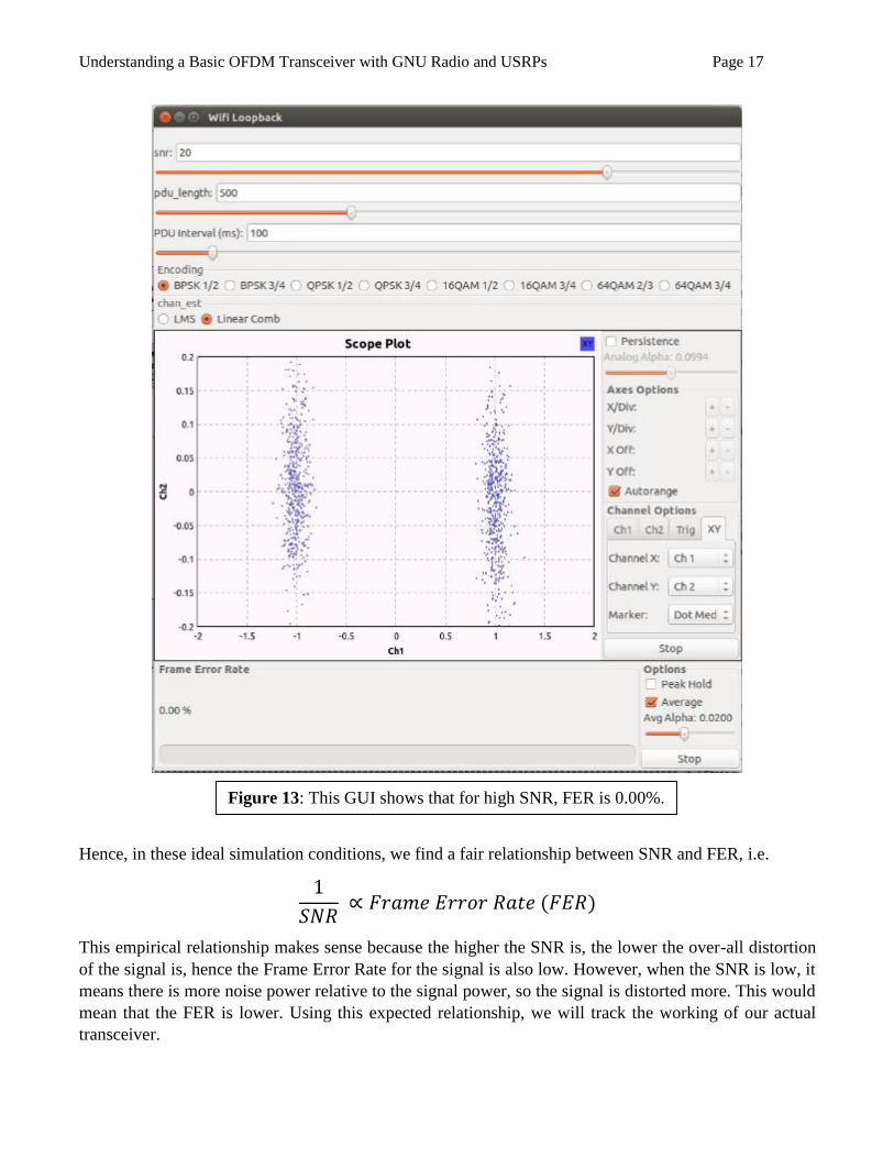
In this ideal simulation, we also find something quite interesting. If we set high values of SNR, we observe

that the Frame Error Rate (FER) stays near 0.0%. But as we begin lowering it, particularly starting around

SNR value of 10, we find that the FER steadily increases.

Figure 12: TX-RX Actual Setup without Co-Axial Cable


Hence, in these ideal simulation conditions, we find a fair relationship between SNR and FER, i.e.

1

𝑆𝑁𝑅 ∝ 𝐹𝑟𝑎𝑚𝑒 𝐸𝑟𝑟𝑜𝑟 𝑅𝑎𝑡𝑒 (𝐹𝐸𝑅)

This empirical relationship makes sense because the higher the SNR is, the lower the over-all distortion

of the signal is, hence the Frame Error Rate for the signal is also low. However, when the SNR is low, it

means there is more noise power relative to the signal power, so the signal is distorted more. This would

mean that the FER is lower. Using this expected relationship, we will track the working of our actual

transceiver.

Figure 13: This GUI shows that for high SNR, FER is 0.00%.


Getting the Actual Transceiver to Work

On the left-hand side Linux machine, we executed the receiver, called “wifi_rx.py”, which was generated

using the flow graphs of “wifi_rx.grc”. This brought up a GUI display with a blank scope plot, which was

not detecting any signals because none were being transmitted in the channel it was listening for. On the

right-hand side Linux machine, we executed the transmitter, call “wifi_tx.py”, and similarly generated by

“wifi_tx.grc”. As soon as we executed the python program, we saw dynamic data show up on the scope

plot of the wifi_rx.py program. This was one sign that the transceiver was working. We also trying to hold

and move around the receiver antenna. This caused a spike in the Frame Error Rate (FER) on the receiver

GUI and the dynamic data also fluctuated immediately. This was a second sign that our transceiver is

functional.

After these simple measures, we were sure that our receiver was working. However, these quick-fix aren’t

enough to confirm that the whole transceiver is functional.

Transmitter and Receiver Signal Plots

We decided to test the functionality of our receiver by plotting the signal that is spit out of the transmitter

and the signal spit out by the receiver. It is important to note that we do not expect both these signals to

be the same, because this is not a simulation. We will analyze the differences in the plots. To plot these,

we need to use MATLAB code which we have included in the Code Appendix.

Let us zoom in on the plot in Figure 14 to analyze the packets slightly better.

Figure 14: First ~1 second of transmitted signal.


Once we zoom in on the plots in Figure 14, we get the plots in Figure 15. For the real values, we can see

a clear repetition pattern at the beginning of the PPDU, denoting the short part of a preamble. If we look

carefully at the following part of the PPDU, we can find a repeating pattern for a long port of the PLCP

preamble. Hence, we have confirmed that the signal coming out of the transmitter is in fact a PLCP

Protocol data unit. This was in fact expected, because given that Bastian Bloessl wrote the flow-graphs in

GNU Radio appropriately, the transmitter should spit out a clear OFDM signal without any signs of

distortion. There is no noticeable distortion from thermal noise, most probably because the signal has

constructed using SDR for the most part. Let us now take a look at the plot of the signal at the receiver.

In Figure 16 on the next page, we see the sheer difference from the plots in Figure 14. The real values do

not look so rich and well distributed, whereas the imaginary values look far too thick. Let us zoon into the

plot to get a better picture.

In Figure 17 we get a better picture of Figure 16 by zooming into those plots. It is hard to find any

resemblance to the plots in Figure 15. This is expected to some extent, but let us try to analyze why the

received signal looks so distorted. For this, let us consider the fact that this received signal, which itself

was captured over a time of roughly 1 second, was captured in the first few seconds of the receiver picking

up the transmitted signal. In these first few seconds, the automated gain control operation is still adjusting

to the power with which the signal hits the receiving antenna. As a result, the FER in the first few seconds

Figure 15: Zoomed first ~1 second of transmitted signal.


Figure 16: First ~1 second of received signal

Figure 17: Zoomed first ~1 second of received signal


of the receiver picking up the transmitted signal is very high (starting at about 90%, and then settling down

over the 5-6 seconds to a low FER). A high FER means that the signal is highly distorted. So in the first

few seconds of the receiver picking up a signal, the distortion is very high. Coincidentally, and quite

unfortunately, it is only within these few starting seconds we captured the signal. The high FER in the

first few seconds is shown in the screenshot in the figure below.

As we can see in Figure 18, the FER is nearly 79%, which is very high. It is no doubt we capture a much

distorted signal during this time. Hence, this begs the question – why not try to capture the received signal

Figure 18: The RX signal in the first few seconds shows a very high FER.


in a time when the Automated Gain Control has adjusted and the FER has settled down? This is possible,

but it would require us to manually tweak the python code of the wifi_rx.py script. Unfortunately we did

not have enough time to try to do this. By default, the GNU Radio Companion GUI simply creates a File

Sink for us, which begins capturing a signal the moment we run the flow graph, and writes it to binary

.dat file, which we can use to plot once we stop executing the flow-graph. The GUI does not give us the

option of capturing a signal after some time has passed. Also, since we only want to handle a small amount

of data (MATLAB takes far too long to process the signal data from longer than one second), we only

capture roughly 1 second of the signal at the beginning of when the flow graph is executed. If we had

more time to work on this project, we would find a way to write and change some of the Python code in

order to begin capturing the signal after a set number of seconds, and only for a single second.

Results Obtained

Now, we try to confirm some SNR relationships through the behavior of the FER as we change distance

between antennae, placing objects in between, and other physical quantities.

Observed SNR Variation in the Line of Sight with Distance

We moved our receiver and transmitter USRP apart by different distances to see how the FER changes.

We made sure that there was a clear direct path between the antennae (line of sight), i.e. there were no

objects blocking the direct path between the receiving and transmitting antennae. The data recorded is

shown in the table below.

Distance

between

antennae (m)

Frame Error

Rate (%)

0.5 1.00

2.5 5.16

5 19.40

7 30.53

Using MATLAB code, we performed a

quadratic fit on this observed data in the

table. The plot is shown to the right.

This code is documented in the Code

Appendix.

Figure 19: A plot that shows a quadratic curve fit

on FER vs. distance points.


In Figure 19, the quadratic regression between the Frame Error Rate (FER) and the distance between the

antennae (R), empirically implies the following proportionality:

𝐹𝐸𝑅 ∝ 𝑅2

But in the simulation of our transceiver we also observed that,

1

𝑆𝑁𝑅 ∝ 𝐹𝐸𝑅

So, we can conclude that,

𝑆𝑁𝑅 ∝1

𝑅2

Which is one of the important takeaways of the Friis Transmission Equation we outlined in an earlier

section of this report. So we see that our transceiver is definitely obeying the Friis transmission equation

and is therefore functioning correctly.

Observed SNR Variation for Path Loss

Our transceiver obeying the Friis transmission equation is a quite a good measure of its functionality, but

let us see how the Frame Error Rate behaves when the line of sight between the Tx and Rx antennae is

blocked by objects, or how the FER behaves in different media. We will try to keep the distance constant

but introduce objects in the line of sight or record the FER in different media.

1) When we measured the FER with a co-axial cable (longer than the one in the picture we have

earlier in the report) connecting the two USRPs, its value was 0.82% (length of the cable was fixed

at about 1 meter)

2) In air, when the antennae are in clear line of sight and 1 m apart, the FER is 1.62%

3) When we put the receiver USRP under the workbench, so the two antennae are blocked by a thick

wooden table, the FER rises to 46.50%. The distance between the USRPs was about 1 meter.

Hence it is quite apparent that within different media and with objects blocking the line of sight, the FER

rises, which means the signal has more noise in it, most probably because of loss of signal power in path

loss. So path loss can decrease the SNR, which is something we outlined earlier.

More Analysis of Results

Now we have come to a point where we know that our transceiver definitely works. However, let’s analyze

our results a little more. We have already analyzed our results for the inverse square law with distance and

the path loss effects. However, in an earlier section of this report, we discussed that SNR can also be

affected by interference, diffraction and noise temperature. Unfortunately do not have an easy way of

measuring the interference or diffraction of the signals from the transmitter USRP. However, during our

experiments, whenever we moved the USRPs, we made sure that their orientation remained the same

when we recorded the data (we maintained an antenna side facing antenna side orientation for the USRPs).

This should be able to give us similar diffraction/interference affects no matter what the distance is. Also,

we can assume that the additive noise temperature throughout our experiments remains the same, because


we are not introducing any new hardware during our experiments which could contribute to increasing

the given thermal noise that already exists for all our hardware. Also, the 0.82% FER that exists even

when the USRPs are connected via co-axial cable can probably be explained by thermal noise.

Possible Future Work

EECS Senior Thesis

Since the student researcher is interested in working in this field further, looking ahead is quite fair. There

is a vast field of opportunity for what can be done in this field. After a discussion with Dr. Dutta about

what lies ahead, we learned that we can use Hardware Description Languages (e.g. VHDL and Verilog)

to program the FPGA in the USRP so that it can spit out data at a far faster rate. CPUs are by default quite

slower than programmed FPGAs, so a USRP can be turned into a powerful device for transmitting and

receiving data. This is because FPGAs perform tasks in parallel processes, whereas CPU perform tasks

sequentially. This research can be used to work toward an EECS Senior Thesis at KU, by applying for

Department Honors in Summer 2016.

Code Appendix

All the code in this section is written in MATLAB.

Signal Reconstruction Code

clear all; clc;

% Author: Arjan Gupta % Purpose: Reconstructing a cosine signal with rectangular pulses

Ts = [0.001, 0.01, 0.05, 0.1]; ta = 0:0.001:1; M = length(ta);

for i = 1:length(Ts)

% cosine signal n = 0:Ts(i):1; N = length(n); x = cos(20*pi*n);

% RECONSTRUCT RECTANGULAR PULSES yrect(i,:) = x*rectpuls(ones(N,1)*ta-[0:N-1]'*Ts(i)*ones(1,M),Ts(i));

% Plot the reconstructed pulses figure(1) subplot(4,1,i) plot(ta,yrect(i,:)) title(sprintf('Rectangular reconstruction for T = %d', Ts(i))); end


PLCP Preamble Construction Code

close all; clc;

% Author: Arjan Gupta % Description: PLCP Preamble Construction

% expected short preamble spreamb = [zeros(1,8), (1+1i), zeros(1,3), (-1-1i), zeros(1,3)]; spreamb = [spreamb, (1+1i), zeros(1,3), (-1-1i), zeros(1,3), (-1-1i), zeros(1,3),

(1+1i), zeros(1,3)]; spreamb = [spreamb, zeros(1,4), (-1-1i), zeros(1,3), (-1-1i), zeros(1,3), (1+1i),

zeros(1,3)]; spreamb = [spreamb, (1+1i), zeros(1,3), (1+1i), zeros(1,3), (1+1i), zeros(1,7)]; spreamb = ((13/6)^(1/2)).*spreamb;

% inverse fast fourier transform of spreamb ifft_spreamb = ifft(spreamb);

% extend ifft_spreamb ifft_spreamb = [ifft_spreamb, ifft_spreamb, ifft_spreamb(1:33)];

% multiply ifft_spreamb by window function ifft_spreamb(1) = 0.5*ifft_spreamb(1); ifft_spreamb(161) = 0.5*ifft_spreamb(161);

% all even values of ifft_spreamb seem to be negative, so let us rectify that for k = 1:length(ifft_spreamb) if (mod(k,2) == 0) ifft_spreamb(k) = ifft_spreamb(k)*-1; end end

% expected long preamble lpreamb = [zeros(1,6), ones(1,2), -1.*ones(1,2), ones(1,2), -1, 1, -1, 1]; lpreamb = [lpreamb, ones(1,5), -1.*ones(1,2), ones(1,2), -1, 1, -1, ones(1,4)]; lpreamb = [lpreamb, 0, 1, -1.*ones(1,2), ones(1,2), -1, 1, -1, 1, -1.*ones(1,5),

1]; lpreamb = [lpreamb, 1, -1.*ones(1,2), 1, -1, 1, -1, ones(1,4), zeros(1,5)];

% inverse fast fourier transform of lpreamb ifft_lpreamb = ifft(lpreamb);

% put the second half of the lpreamb in front ifft_lpreamb = [ifft_lpreamb(33:end), ifft_lpreamb(1:32)];

% extend ifft_spreamb ifft_lpreamb = [ifft_lpreamb, ifft_lpreamb, ifft_lpreamb(1:33)];

% multiply ifft_lpreamb by window function ifft_lpreamb(1) = 0.5*ifft_lpreamb(1); ifft_lpreamb(161) = 0.5*ifft_lpreamb(161);

% all even values of ifft_lpreamb seem to be negative, so let us rectify that


for k = 1:length(ifft_lpreamb) if (mod(k,2) == 0) ifft_lpreamb(k) = -1*ifft_lpreamb(k); end end

preamble = [ifft_spreamb(1:160), (ifft_spreamb(161)+ifft_lpreamb(1)),

ifft_lpreamb(2:160)];

% Ideal PLCP preamble in IEEE 802.11 WLAN! figure abs_preamb = abs(preamble); plot(1:320,abs_preamb); legend('Expected PLCP preamble');

TX Captured Signal Plot Code

close all; clc;

% Author: Arjan Gupta % Description: USRP tx packet samples analysis

% This code reads and plots the USRP samples fh = fopen('data.dat', 'rb'); data = fread(fh,'int16'); cdata = complex(data(1:2:end),data(2:2:end)); fclose(fh); re = real(cdata); img = imag(cdata);

figure subplot(2,1,1) plot(re) title('Real values of transmitted signal'); subplot(2,1,2) plot(img) title('Imaginary values of transmitted signal');

RX Captured Signal Plot Code

close all; clc;

% Author: Arjan Gupta % Description: USRP rx packet samples analysis

% This code reads and plots the USRP samples fh = fopen('data_rx.dat', 'rb'); data = fread(fh,'int16'); cdata = complex(data(1:2:end),data(2:2:end)); fclose(fh); re = real(cdata); img = imag(cdata);

figure


subplot(2,1,1) plot(re) title('Real values of received signal'); subplot(2,1,2) plot(img) title('Imaginary values of received signal');

FER vs. Distance Plot Code

close all; clc;

% Author: Arjan Gupta % Purpose: Plot the FER vs. distance

distances = [0.5, 2.5, 5, 7]; FERs = [1, 5.16, 19.40, 30.53];

p = polyfit(distances,FERs,2); x1 = linspace(1,10,19); y1 = polyval(p,x1); figure stem(distances,FERs,'o'); hold on plot(x1, y1) hold off xlabel('Distance (m)'); ylabel('FERs (%)'); legend('Observed data','Quadratic fit for FER vs. distance');


Bibliography

Works Referenced

[1] Malik, Bilal. "Analog to Digital Converter and How ADC Works." (n.d.): n. pag. Micro Controllers

Lab. 31 July 2013. Web. 16 May 2016. <http://microcontrollerslab.com/analog-to-digital-adc-

converter-working/>.

[2] Adat, Rachad. "EECS 360 Signal and System Analysis Lab 10: Sampling and Signal Reconstruction."

Web. 17 May 2016. <http://people.eecs.ku.edu/~esp/class/S16_360/lab/Lab10ATAT.pdf>

[3] Information technology--Telecommunications and information exchange between systems Local and

metropolitan area networks--Specific requirements Part 11: Wireless LAN Medium Access

Control (MAC) and Physical Layer (PHY) Specifications," in ISO/IEC/IEEE 8802-11:2012(E)

(Revison of ISO/IEC/IEEE 8802-11-2005 and Amendments), vol., no., pp.1-2798, Nov. 21 2012.

22 March 2016. doi: 10.1109/IEEESTD.2012.6361248

<http://standards.ieee.org/getieee802/download/802.11-2012.pdf>

[4] "USRP™ N200/N210 Networked Series." (n.d.): n. pag. Ettus Research. Web. 15 May 2016.

<www.ettus.com>.

[5] Šolc, Tomaž. USRP N210 with SBX and top cover off. Digital image. Tablix. N.p., 07 June 2012.

Web. 14 May 2016. <https://www.tablix.org/~avian/blog/articles/about/>.

[6] Bloessl, Bastian, Michele Segata, Christoph Sommer, and Falko Dressler. "An IEEE 802.11a/g/p

OFDM Receiver for GNU Radio." (n.d.): n. pag. Institute of Computer Science, University of

Innsbruck, Austria, Dept. of Information Engineering and Computer Science, University of Trento,

Italy, Mar. 2013. Web. 20 Mar. 2016. <http://www.ccs-labs.org/bib/bloessl2013ofdm-tr/>.

usrp project final report

Documents