Using Whispering Gallery Mode Resonators to Accurately Track

Temperature Fluctuations

Bain Alexander BronnerAdviser: Dr. Eugeniy Mikhailov

Abstract

Whispering Gallery Mode Resonators (WGMRs) are optical resonant cavities. By

producing high Q-factor disks, the aim is to create miniature sensors which are able to

track environmental variables (such as temperature) with high precision. Fabrication of

the disks and coupling into the resonators is outlined and studied as well. A Q > 108

has been produced in this study, as well as coupling of over 60%. We were able to

resolve temperature shifts down to about 500 nK, limited by electronic noise. Future

outlooks are also mentioned.

1 Introduction

The main purpose of this experiment was to realize precise measurements of temperature

change, by tracking an optical resonant cavity. The optical cavities used were Whispering

Gallery Mode Resonators (WGMRs), which can store light for long periods of time, with

little loss [1]. The main interest was to use the resonant modes to keep track of the radius

of the disk. Whilst knowing the thermal expansion coefficient and the change in the index

of refraction with temperature [2], the change in size, and thus the temperature shift, of the

resonant volume could be calculated.

The traditional Fabry-Perot (FP) resonator, while useful in many applications, is not

well suited for this kind of measurement. High quality FP resonators tend to be expensive,

complex, and prone to vibration instabilities due to low-frequency mechanical resonances.

1

For this application, the stability and relatively small size of the resonator are very important

[3]. The response time is directly related to the heat capacity of the resonator, thus smaller

resonators will have a faster response. Further, any instabilities in the resonator would

degrade measurement capabilities.

Whispering gallery mode resonators lend themselves well to this kind of measurement.

These disk can be fabricated with a very high Quality Factor (Q-factor, defined in Equa-

tions (1) and (2)). High Q-factor’s imply narrow resonant widths as well as longer lifetimes

for the resonating wave. Thus optical path lengths of hundreds or thousands of meters are

created. Q-factors of 1011 have been reported [4], while Q’s in excess of 108 have been pro-

duced in our lab. Further, the small size of WGMRs allow them to respond fairly quickly to

changes in the environment. Therefore, they were chosen for this measurement/experiment.

2 Theory

Q-factor and finesse are the two most important quantities when discussing resonators. Be-

ginning with Q-factor, it is defined as follows:

Q ∼ Energy Stored

Energy Dissipated per Cycle, (1)

however, to actually measure it for a given resonator, it can be defined as:

Q =ν0

∆ν= ν0Trt

2π

l, (2)

which is valid in the high Q regime. In Equation (2), ν0 is the frequency of the light and ∆ν

is the mode’s full-width at half-maximum. Trt is the round trip time i.e. one trip around the

circumference of the disk, and l is the loss. From that equation, one can see that narrower

mode widths correspond with higher Q-factors, as well as diminishing losses.

Finesse, on the other hand, is a measure of the free spectral range (FSR) divided by the

2

mode width. The FSR of a given resonator is defined as:

FSR =c

4nπR, (3)

where c is the speed of light, n is the index of refraction of the resonator, and R is the radius

of the disk [5]. As can be seen in Equation (3), smaller disks have a larger free spectral

range. Finesse is related to the Q-factor by:

F =λQ

neffLcav

, (4)

where neff is the effective index of refraction and Lcav is the path length. For disk resonators,

Lcav = 2πR, where R is the radius of the disk. From this point, the focus will be on the

more easily measured quantity, the Q-factor.

To measure temperature changes, we track the resonant modes’ position, given by this

formula:

ν = mc

2πRTnT

, (5)

where the radius of the disk (R) and the index of refraction (n) are both temperature depen-

dent, and m is the mode number. Thus, the resonance position is a function of temperature,

and we can calculate changes in T , by knowing the shift in resonance frequency, using:

∆T =−∆ν

ν0

(n ∂n

∂T+ α

) , (6)

where ∂n/∂T is the change in the index of refraction with respect to temperature, α is the

thermal expansion coefficient, and ν0 is the unperturbed resonant frequency. Rearranging

Equation (6), the change in frequency per degree Celsius is:

∆ν

∆T= −ν0

(n∂n

∂T+ α

)= γν0, (7)

3

where γ is used to denote the proportionality constant. The accuracy of the temperature

measurement is related to the accuracy of the measured resonance shift (∆ν). Since Q-factor

and mode width are inversely related, and changes in temperature are directly proportional

to mode shift, higher Q-factors are desirable for greater precision in tracking temperature

changes. This can be readily seen with the following thought experiment: if a given mode is

300 MHz wide, then a shift of 3 MHz is only 1% of the total width. However, a mode that

is 3 MHz wide would shift by its entire line-width. Thus, for a given change in temperature,

narrower modes are desired.

Increasing Q-factors imply longer optical path lengths, as can be seen by combining

Equations (2) and (4). Therefore, smaller changes to the disk size become more noticeable,

leading to an ability to track smaller variations in temperature. Further, by utilizing a

laser-lock, shifts in frequency can be measured in fractions of the mode width.

3 Resonator Fabrication and Coupling

Calcium fluoride (CaF2) and lithium niobate (LiNbO3) WGMR disks have been produced.

The disks were created by drilling circular blanks out of a crystalline window, and then

mounting them onto brass posts. Subsequent rounds of shaping and polishing were done on

a lathe using progressively finer lapping paper, while cleaning the disks with acetone between

steps. The final two steps involved using a 0.5 µm and 0.1 µm diamond emulsion fluid. An

example of polished and shaped disks we’ve used is in Figure 1. Using this procedure, a

Q-factor greater than 108 has been produced with a LiNbO3 disk.

The next step is coupling, or actually getting light into the resonator. To achieve critical

coupling, the waveguide to resonator power must exactly match any intrinsic losses [6].

Whispering gallery mode resonators can be coupled into by a few different methods. In this

case, prism coupling with both a rutile (TiO2) and diamond prism were used, at different

points. The diamond prism is shown in Figure 2. As can be seen in the picture, the prism

4

(a) A Calcium Fluoride WGMR, 7mm in diameter(Q ' 1× 107)

(b) A Lithium Niobate WGMR, 7mm in diameter(Q ' 1.5× 108)

(c) A Potassium Lithium Niobate WGMR,0.66mm in diameter (Polished by JPL, Q ∼ 107)

(d) A Lithium Niobate WGMR, 1.6mm in diam-eter (Polished by JPL, Q ' 5× 107)

Figure 1: Assorted WGMRs

5

Figure 2: Diamond prism with ruler in background. The largest tick mark corresponds toone centimeter

faces are less than two millimeters wide. Prism coupling is based on a few principles. The first

is the evanescent wave. At the point of total internal reflection, an exponentially decaying

wave exists outside of the prism-air interface. This follows from the boundary condition that

the electric field must be continuous at the boundary; that is, ~Eincoming+ ~Ereflected = ~Etransmitted

[7]. By placing the disk in this region, frustrated total internal reflection, can take place,

which is analogous to quantum mechanical tunneling. Thus, power can be transmitted from

the prism to the resonator.

In addition, the input beam needs to be focused inside the prism at an angle that provides

phase matching between the evanescent wave of the total internal reflection spot and the

WGMR, respectively. The angle that meets this requirement satisfies the following:

sinφ ' nr

np

, (8)

6

where φ is the critical angle, nr is the index of refraction of the disk resonator, and np is

the index of refraction of the prism [6]. See Figures 3 and 4 for an illustration, and Figure 5

for a picture of two actual disk/prism combinations. Appendix B contains similar plots for

other disk/prism combinations used in this study.

Figure 3: Coupling diagram generated with our code: φ = 34.57◦

Figure 4: Beam trace generated with our code; the opacity of the beam indicates relativeintensity

7

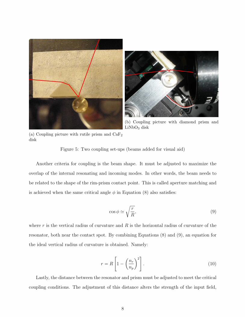
(a) Coupling picture with rutile prism and CaF2

disk

(b) Coupling picture with diamond prism andLiNbO3 disk

Figure 5: Two coupling set-ups (beams added for visual aid)

Another criteria for coupling is the beam shape. It must be adjusted to maximize the

overlap of the internal resonating and incoming modes. In other words, the beam needs to

be related to the shape of the rim-prism contact point. This is called aperture matching and

is achieved when the same critical angle φ in Equation (8) also satisfies:

cosφ '√r

R, (9)

where r is the vertical radius of curvature and R is the horizontal radius of curvature of the

resonator, both near the contact spot. By combining Equations (8) and (9), an equation for

the ideal vertical radius of curvature is obtained. Namely:

r = R

[1−

(nr

np

)2]. (10)

Lastly, the distance between the resonator and prism must be adjusted to meet the critical

coupling conditions. The adjustment of this distance alters the strength of the input field,

8

since the evanescent field exponentially decays with distance from the prism. When the

input field provides more power than is lost in the resonator, it is said to be “over-coupled;”

when the internal losses are greater than the incoming field, it is said to be “under-coupled.”

However, it should be noted that some loss in the form of an output field is required in order

to make measurements.

The coupling level is described by the mode absorption relative to the mean voltage of the

output signal. Figure 6 shows a coupling level from this experiment. The general procedure

used to achieve coupling follows:

• To initially get the beam spot focused on the disk, the angle was set to slightly less than

the critical angle. That is, it was set so that the beam would not totally-internally-

reflect, but rather refracted into the resonator. Once the disk-prism contact spot was

found by observing illumination of the disk, the angle was adjusted to the critical point.

• The best horizontal angle was usually slightly different from the theoretical predictions.

The best angle was found by searching around the predicted one. Q-factor would not

increase or decrease during this time, rather the coupling level would go up and down.

Once this angle was optimized, attention turned to the vertical angle of the prism.

• The vertical angle of the coupling prism played a large role in the coupling level; very

small changes had drastic effects. By adjusting this angle in small amounts, the angle

of the probe beam was adjusted to be parallel with the disk-rim plane. Once again,

coupling contrast was optimized.

• The focal length of the lens (and the subsequent beam waist size) used also made a

significant difference in coupling. After time, the most effective technique for deter-

mining the appropriate lens became viewing the emission beam on a sheet of paper,

through an infrared viewer. As the resonator was brought into coupling, the size of the

beam spot compared to the contact spot size could be observed. If the contact spot

9

Figure 6: Coupling voltage differences

was smaller than the beam, a shorter focal length was employed; if the opposite was

observed, a larger focal length was used.

• Using these techniques, a mode-contrast of almost 70% has been observed.

4 Results

Initially, research was focused on increasing the Q-factor to allow for precise measurements.

After much trial and error, a procedure was developed which allowed for the creation of a

WGMR disk with Q > 108. The full procedure is listed in Appendix A. An example of the

resonant modes is in Figure 7.

During the same time as Q-factor experiments, various measurements were taken of

the disk rim. The horizontal radius of curvature was easily measured using a microscope,

however measuring the vertical radius of curvature is difficult using the same technique, since

the vertical radius is not continued for the whole disk; it is a curvature localized to the rim.

10

Figure 7: Whispering Gallery Modes with 87Rb Spectra

Alternatively, in order to get an accurate idea of the shape of the disk, Newton rings were

observed reflecting off of the contact point. By making the probe beam significantly larger

than the contact spot, rim shape could be deduced. The resulting Newton rings were able

to depict both the vertical and horizontal radius through the following relation:

rN =

[(N − 1

2

)λR

]1/2

, (11)

where N is the bright ring number, λ is the wavelength of light, and R is the radius of

curvature. One of these pictures is in Figure 8. In order to estimate the curvature, the

optical elements between the disk and camera need to be taken into account.

Another venture into the properties of WGMRs was done by changing the polarization of

the probe beam. It was found that polarization in the plane of the disk produced narrower

modes than vertical polarization. The difference was about a factor of three, which can

be seen in Figure 9. To rule out time-degradation of the disk, these measurements were

conducted within 30 minutes of one another.

11

Figure 8: Newton’s rings produced by a WGMR disk

5 Temperature Tracking

After those initial tests, temperature tracking was done visually on an oscilloscope, using

a thermistor as a reference. This was done for both CaF2 and LiNbO3. Using reported

values for ∂n/∂T and α [8], an expected response of 4.21 GHz/K was calculated for CaF2.

The measured shifts in resonant position were: 4.13, 4.10, and 3.91 GHz/K. The average

for these measurements was 4.05 GHz/K, which was in good agreement with the expected

value. A similar test was done with LiNbO3. A plot containing the temperature change

measured by a thermistor and the resonance position is in Figure 10.

After testing of the concept and demonstrating that it followed the theory, a lock-in

amplifier was employed to electronically track mode position. By measuring the feedback

12

(a) Horizontal Polarization (plane of the disk) (b) Vertical Polarization

Figure 9: Comparing modes (a) and (b), the difference in width can be seen. It was abouta factor of three.

signal, the relative mode shift can be calculated, and then converted into a temperature

change. To calculate the smallest voltage change that could be attributed to temperature

shift, the noise level of the signal had to be taken into account. The signal-to-noise ratio

provides the level to which one could resolve any changes. The following formula provides

the smallest temperature change that can be measured in this way:

∆Tbest =2

SNR

∆ν

γ(12)

where SNR is the signal-to-noise ratio, ∆ν is the mode width, and γ is the frequency to

temperature relation from Equation (7). The factor of 2 comes from the response signal

being twice the mode width at half-maximum. Initially, a noise level of 20 mV was measured,

with an error signal of 20 V , yielding an SNR of 1000. The mode width at this time was 5

MHz. Plugging these values into Equation (12), along with the measured γ of 2.65 GHz/K

for LiNbO3, yielded a ∆Tbest of 3.8 µK. However, after the addition of a neutral density

filter, the noise level remained the same 20 mV , while the error signal amplitude was 15%

of its original value. Therefore, by multiplying the new error signal by 6.67, the real signal

amplitude was obtained. Using this new value of Verror = 133.4 V , while the same error

13

Figure 10: Temperature tracking uses mode position

14

Figure 11: The response signal along with the mode being tracked. The noise in the modeis due to dithering the laser

signal width and noise level was seen, yielded a new ∆Tbest ' 570 nK. See Figure 11 for a

response curve.

6 Conclusions and Outlooks

The ability to track changes in temperature on the level of 0.5 µK was demonstrated. Given

different crystals with higher changes to temperature and/or higher Q-factors, even greater

precision could be accomplished. In this experiment, the noise level remaining at 20 mV

after inclusion of a neutral density filter, indicated that the noise was due to electronics. By

taking noise to the shot-noise level, large improvements could be made. Q-factors of 1011

have been demonstrated, and this would also lower the smallest change able to be tracked

by decreasing the mode-width. For example, a CaF2 disk with Q ∼ 109 would increase

the temperature response by a factor of 1.5 and lower the mode-width by a factor of ten,

resulting in tracking down to about 40 nK.

15

Further, while temperature was the variable tracked in this experiment, any environ-

mental factor could likewise be tracked, assuming it affects the resonator in a measurable

way. These factors include pressure, electric field strength, and frequency just to name a

few. Also, the small size and relative durability of these disks lend them to be used on

chips or in locations that a Fabry-Perot resonator would be impractical. The relative ease

of manufacture and low expense further enhances their appeal.

7 Acknowledgments

The author would like to thank Eugeniy Mikhailov for his guiding support throughout this

process, Irinia Novikova for her helpful insight into problems, and Matthew Simons for his

patience and entertaining conversations.

References

[1] Vladimir S. Ilchenko, Anatoliy A. Savchenkov, Andrey B. Matsko, and Lute Maleki.Nonlinear optics and crystalline whispering gallery mode cavities. Phys. Rev. Lett.,92:043903, Jan 2004.

[2] Liron Stern, Ilya Goykhman, Boris Desiatov, and Uriel Levy. Frequency locked micro diskresonator for real time and precise monitoring of refractive index. Opt. Lett., 37:1313–1315, Apr 2012.

[3] A.B. Matsko and V.S. Ilchenko. Optical resonators with whispering-gallery modes-parti: basics. Selected Topics in Quantum Electronics, IEEE Journal of, 12(1):3–14, 2006.

[4] Anatoliy A. Savchenkov, Andrey B. Matsko, Vladimir S. Ilchenko, and Lute Maleki.Optical resonators with ten million finesse. Opt. Express, 15(11):6768–6773, May 2007.

[5] N. Hodgson and H. Weber. Optical Resonators: Fundamentals, Advanced Concepts, andApplications. Springer Verlag, 1997.

[6] Lute Maleki, Vladimir S . Ilchenko, Anatoliy A . Savchenkov, and Andrey B . Matsko.Practical Applications of Microresonators in Optics and Photonics. CRC Press, 2009.

[7] H.J. Pain. The physics of vibrations and waves. John Wiley & Sons Canada, Limited,1999.

16

[8] D. N. Batchelder and R. O. Simmons. Lattice constants and thermal expansivities of sili-con and of calcium fluoride between 6[degree] and 322[degree]k. The Journal of ChemicalPhysics, 41(8):2324–2329, 1964.

17

Appendices

A Polishing Technique

Polishing procedure:

1) Starting from a cut blank, 600 grit aluminum oxide sandpaper was used to remove ma-

terial from the edge due to any cracks formed during cutting, using water as a lubricant.

The lathe was set to approximately 50% of maximum speed, as indicated on the knob.

Then, the sand paper was attached to a glass plate and used to bevel both the top and

bottom edge until they met at a point, forming the rim. The angle of the bevel on the

bottom edge was limited by the post, but a top and bottom bevel of ≈ 45◦ was used.

After this step, the disk was rinsed with water and dried.

2) Next, the beveling was continued in the same fashion with 1000 grit aluminum oxide

sandpaper, once again using water as a lubricant, removing more material, and making

the edge finer. The lathe speed was still at about 50%. The time for this and the previous

step depended on the amount of material to be removed. After practice, it became clear

to not use too much pressure, as this created deep gouges in the disk. Once satisfied by

the evenness of the surfaces after examination under a microscope, the disk was again

cleaned.

3) The next step moved to 30 µm particle-size lapping paper. Lathe speed was lowered to

about 40%. A methanol based polishing solution was used as a lubricant and for rinsing.

Continuing use of a glass plate, the bevel and surface continued to be polished/shaped.

The rim itself remained untouched. After the surface again looked even under the micro-

scope, albeit with smaller imperfections, the disk was rinsed and dried.

4) The next size lapping paper was 9 µm. The methanol polishing solution was still used,

and lathe speed was the same as in the previous step. This step continued as the previous

18

ones, taking the surface to an even finer smoothness. The rim was still not touched, and

the glass plate was still used as a backer. After this step, the rim had become very sharp,

and the disk was rinsed and dried.

5) Moving to a 3 µm lapping paper, the methanol polishing solution was still used, but the

glass plate was discontinued. Lathe speed remained as it was in the previous two steps.

Attention now moved to the rim. The lapping paper was held to allow it to come into

contact with a quarter to a fifth of the rim surface. It was then moved back-and-forth

over the rim, beginning to round it. The rest of the disk was ignored at this point, since

it played no part in the quality of the resonator. The time for this step was somewhat

variable, but after two minutes of proper polishing, the rim was usually ready for the

next step. To check this, the disk was first rinsed with the polishing solution, dried, then

rinsed with optically clean (pure) acetone, and dried once again. The acetone removed

the oily residue left by the polishing solution, allowing one to see imperfections. The

surface blemishes along the rim were small now, but still visible. Any blemishes about

the same size of the rim needed to be removed during this step, so if any existed, this

step was repeated until they were gone.

6) The last lapping paper size used was 1 µm. Lathe speed was still about 40% and the

polishing solution was still used. In the same way as the previous step, the rim was

polished. Once again, two minutes was a usual time. The same rinse with polishing

solution, dry, rinse with acetone, and dry procedure was done before viewing it under the

microscope. At this point, the disk rim had been slightly broadened by the polishing and

was also somewhat curved. All the marks on the rim were just visible at this point, and

if not, this step was repeated until that was the case.

7) The methanol polishing solution was no longer used from this point forward. In this step,

a 0.5 µm particle size diamond emulsion was used to polish. A wipe was dampened with

this fluid, then cupped around the disk. Lathe speed was slightly lowered, to about 30%.

19

After one minute, more of the solution was added to the cup created by the wipe, creating

a pool of fluid in which the disk rotated, and it was polished for another minute. During

this step, the pressure used holding the wipe to the disk was somewhat firm. When too

much pressure was used, the wipe would tear, and start to wrap around the disk/post,

creating a potential for the disk to become disconnected from the post. However, after

several polishing sessions and mishaps, a feeling for the correct pressure was found. Note:

due to an oversight during the first time using the emulsions, acetone was not used to

clean the disk between this and the next step. However, because that disk yielded the

highest Q-factor yet produced in our lab (∼ 8× 107), superstition kept that same habit

for subsequent polishings. On the next polishing following this oversight, Q > 108 was

measured. It is not clear if the acetone cleaning at this stage has either no effect, limits

the production of higher Q-factors, or is in some way beneficial.

8) Lastly, a 0.1 µm diamond emulsion was used. The first two minutes of this step proceed in

the exact same way as the previous, however after two minutes, lathe speed was lowered

to 20% speed or so. As the third minute progressed, fluid was added to keep the disk in a

“pool.” Further, the speed was gradually lowered throughout, eventually to the point of

stopping, around the three minute mark. The disk was then cleaned with acetone, dried,

and examined. At this point, any rim imperfections were too small to see with an optical

microscope. If there were some remaining, then depending on their size, the procedure

was picked up from one of the previous steps. Knowing exactly where to re-start came

with experience after many polishing sessions.

Extra Notes:

• Both broad and narrow rims have been produced. Narrow rims have yielded higher

Q-factors and better mode isolation, that is, less overlapping with nearby modes.

20

B Coupling Plots

These plots show the coupling parameters for a LiNbO3 disk with a diamond prism.

Figure 12: Coupling Angles

Figure 13: Beam Trace

21