using the nag toolbox for matlab in mathematical finance · 2019-02-22 · using the nag toolbox...

Using the NAGToolbox forMATLAB

in Mathematicalfinance

NicolettaGabrielli

Heston ModelParameters

Pricing formulae

Option pricing withFFT

Variance GammaModelDefinition

Simulation

Implicit Formula forimplied volatility

Using the NAG Toolbox for MATLABin Mathematical finance

Nicoletta Gabrielli

May 14, 2010



NicolettaGabrielli


Pricing formulae



Simulation


Outline

1 Heston ModelParametersPricing formulaeOption pricing with FFT

2 Variance Gamma ModelDefinitionSimulationImplicit Formula for implied volatility



NicolettaGabrielli


Pricing formulae



Simulation


Heston

The Heston Model

dSt = µStdt +√

VtStdWt

dVt = κ(θ − Vt )dt + σ√

VtdZt

dWtdZt = ρdt

where{St}t≥0 and {Vt}t≥0 are price and volatility processes{Wt}t≥0 and {Zt}t≥0 are Wiener processes with correlation ρθ is long-run mean, κ is the rate of reversion and σ is volatilityof volatility



NicolettaGabrielli


Pricing formulae



Simulation


Outline





NicolettaGabrielli


Pricing formulae



Simulation


Black Scholes Implied Volatility

A European call option on an asset St , paying no dividends,with maturity date T and strike price K is defined as acontingent claim with payoff max(ST − K ,0) at maturityThe Black-Scholes formula for the value of this call option is:

CBS(St ,K , τ, σ) = StN(d1)− Ke−rτN(d2) (1)

d1 =− log x + τ(r + σ2

2 )

σ√τ

, d2 =− log x + τ(r − σ2

2 )

σ√τ

(2)

where τ = T − t , x = K/St and N(u) is the normalcumulative distribution function.If C∗t (T ,K ) are the market prices, there exists a uniquevolatility parameter σBS(T ,K ) such that the correspondingBlack-Scholes prices match the market price:

∃!σBS(K ,T ) > 0 : CBS(St ,K , τ, σBS(T ,K )) = C∗t (T ,K ).



NicolettaGabrielli


Pricing formulae



Simulation


κ and σ

From empirical studies we can see that asset’s log-returndistribution has heavy tails and high peaksSuch distribution can’t be Normal, as assumed in theBlack-Scholes modelσ affects the kurtosis of the log-returns distribution.

σ = 0 means constant volatility and so there is no skewHigher values of σ make the skew/smile more prominent

kappa is the mean reversion parameter

Figure: Parameters used are θ = 0.04, ρ = 0, v0 = 0.04, r = 0.01,S = 1



NicolettaGabrielli


Pricing formulae



Simulation


Impact of ρ on volatility surfaces

ρ in Heston Model can be seen as the correlation betweenlog-returns and asset volatilitydifferent values of ρ change heaviness of the tails

Changes in skewness imply different shapes of the impliedvolatility surface

Figure: Implied volatility surfaces for ρ = −0.5, 0, 0.5. Parameters andvariables used are κ = 2, θ = 0.04, σ = 0.1, v0 = 0.04, r = 0.01,S = 1

See [Moo05]



NicolettaGabrielli


Pricing formulae



Simulation


Outline





NicolettaGabrielli


Pricing formulae



Simulation


Heston prices with s30na

s30na computes the European option price given by Heston’sstochastic volatility model

[p, ifail] = s30na(calput, x, s, t, sigmav, ...kappa, corr, v0, eta, gamma, ...r, q, ’m’, m, ’n’, n)

The option price is computed by evaluating the integral transformgiven by Lewis in [Lew01]:

C(S,K ,T ) = Se−qT−√

SKπ

e−T2 (r+q)

∫ ∞0Re(

eiukφT (u− i2

)) du

u2 + 14

.

(3)where, see [Sch03]

φT (u) = exp[ θκσ2

((κ− rhoσu − d)T − 2 log

1− ge−dT

1− g

)+

v02

θ2(κ− rhoσiu − d)

1− e−dT

1− ge−dT

]d =

√(ρσui − κ)2 + θ2(iu + u2), g =

κ− ρσiu − dκ− ρσiu + d



NicolettaGabrielli


Pricing formulae



Simulation


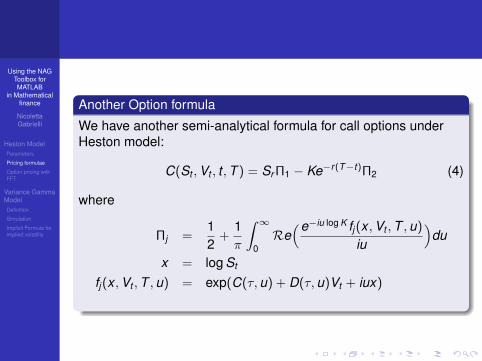
Another Option formula

We have another semi-analytical formula for call options underHeston model:

C(St ,Vt , t ,T ) = Sr Π1 − Ke−r(T−t)Π2 (4)

where

Πj =12

+1π

∫ ∞0Re(e−iu log K fj (x ,Vt ,T ,u)

iu

)du

x = log St

fj (x ,Vt ,T ,u) = exp(C(τ,u) + D(τ,u)Vt + iux)



NicolettaGabrielli


Pricing formulae



Simulation


Parameters in (4) are:

C(τ,u) = rui +aσ2

[(bj − ρσui + d)τ − 2 log

1− gedr

1− g

]D(τ,u) =

bj − ρσui + dσ2

( 1− edr

1− gedr

)g =

bj − ρσui + dbj − ρσui − d

d =√

(ρσui − bj )2 − σ2(2cjui − u2)

c1 =12, c2 = −1

2,a = κθ,b1 = κ+ λ− ρσ, b2 = κ+ λ



NicolettaGabrielli


Pricing formulae



Simulation


Outline





NicolettaGabrielli


Pricing formulae



Simulation


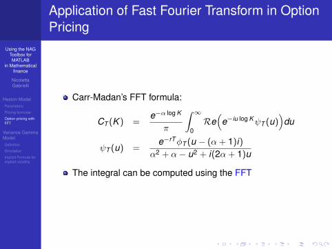
Application of Fast Fourier Transform in OptionPricing

Carr-Madan’s FFT formula:

CT (K ) =e−α log K

π

∫ ∞0Re(

e−iu log KψT (u))

du

ψT (u) =e−rTφT (u − (α + 1)i)

α2 + α− u2 + i(2α + 1)u

The integral can be computed using the FFT



NicolettaGabrielli


Pricing formulae



Simulation


FFT is an algorithm used to calculate summations of thefollowing form:

w(k) =N∑

j=1

e−i 2πN (j−1)(k−1)x(j) (5)

Carr-Madan formula

CT (ku) ' −αku

π

N∑j=1

e−i 2πN (j−1)(u−1)eibvjψT (vj )

η

3(3 + (−1)j − δj−1)

(6)



NicolettaGabrielli


Pricing formulae



Simulation


NAG routine for FFT

c06ec calculates the discrete Fourier transform of a sequence ofn complex data values defined by:

wk =1√N

N∑j=0

ei2πjk

N xj k = 0,1, . . . ,N − 1.

Figure: The comparison between prices evaluated with FFT and valuesfrom s30na: κ = 2, θ = 0.04, σ = 0.1, v0 = 0.04, r = 0.01,S = 100η = 0.15,N = 4096



NicolettaGabrielli


Pricing formulae



Simulation


Outline





NicolettaGabrielli


Pricing formulae



Simulation


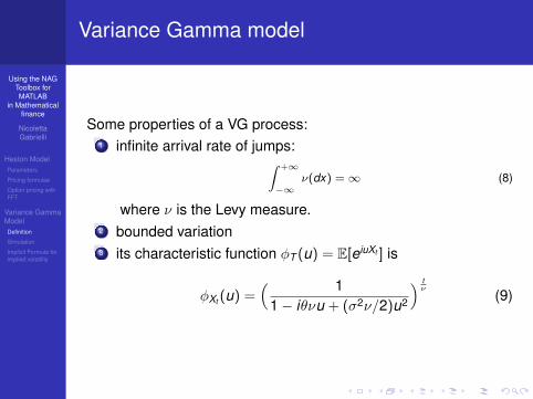
Variance Gamma model

VG process

A Variance Gamma process is a stochastic process {Xt}t≥0

Xt = θΓt + σWΓt (7)

where{Wt}t≥0 is a Wiener process{Γt}t≥0 is a gamma process with unit mean and variance ν



NicolettaGabrielli


Pricing formulae



Simulation


Variance Gamma model

Some properties of a VG process:1 infinite arrival rate of jumps:∫ +∞

−∞ν(dx) = ∞ (8)

where ν is the Levy measure.2 bounded variation3 its characteristic function φT (u) = E[eiuXt ] is

φXt (u) =( 1

1− iθνu + (σ2ν/2)u2

) tν

(9)



NicolettaGabrielli


Pricing formulae



Simulation


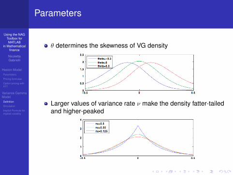
Parameters

θ determines the skewness of VG density

Larger values of variance rate ν make the density fatter-tailedand higher-peaked



NicolettaGabrielli


Pricing formulae



Simulation


Parameters

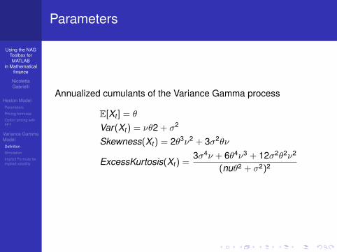
Annualized cumulants of the Variance Gamma process

E[Xt ] = θ

Var(Xt ) = νθ2 + σ2

Skewness(Xt ) = 2θ3ν2 + 3σ2θν

ExcessKurtosis(Xt ) =3σ4ν + 6θ4ν3 + 12σ2θ2ν2

(nuθ2 + σ2)2



NicolettaGabrielli


Pricing formulae



Simulation


Outline





NicolettaGabrielli


Pricing formulae



Simulation


Algorithm1 Fix a time grid t1 . . . tn2 Simulate n independent gamma variables ∆Si with

parameters ti−ti−1ν , ν

3 Simulate n i.i.d. N(0,1) random variables Ni

4 Set ∆Xi = θ∆Si + σNi√

∆Si

The discretized trajectory is X (ti ) =∑i

k=1 ∆Xi

See [CT04]



NicolettaGabrielli


Pricing formulae



Simulation


VG process as difference of two gammaprocesses

φXt (u) = etη(u) with η(u) = ν log(

1− iθνu + (σ2ν/2)u2)

(1− iθνu + (σ2ν/2)u2

)=(

1− iuα(1)

)×(

1 + iuα2

)with

α(1) =(1

2ν

√θ2 +

2σ2

ν+

12θ)−1

and α(2) =(1

2ν

√θ2 +

2σ2

ν− 1

2θ)−1

If Γt is a gamma process with parameters α and β itscharacteristic function is

φΓt (u) =(

1− iuα

)−βXt has the same law as the difference of two independentgamma subordinators with respective parameters α(1) andβ(1) = 1/ν, α(2) and β(1) = 1/νThese two gamma processes can be seen as moves up anddown of stock

See [Kyp07]



NicolettaGabrielli


Pricing formulae



Simulation


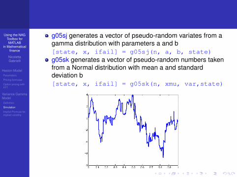
g05sj generates a vector of pseudo-random variates from agamma distribution with parameters a and b[state, x, ifail] = g05sj(n, a, b, state)g05sk generates a vector of pseudo-random numbers takenfrom a Normal distribution with mean a and standarddeviation b[state, x, ifail] = g05sk(n, xmu, var,state)



NicolettaGabrielli


Pricing formulae



Simulation


DefinitionVariance Gamma model is the exponential Levy model obtainedfrom a Variance Gamma process.

The risk-neutral dynamics is given by

St = S0 exp[(r + ω)t + Xt

](10)

where

ω =1ν

log(

1− θν − σ2ν

2

)



NicolettaGabrielli


Pricing formulae



Simulation


Monte Carlo simulation and VG prices

We value European calls with Monte Carlo method using 15000simulations and compare them with the analytic formula inMadan-Carr-Chang article.

Maturity Explicit Monte Carlo0.25 3.4742 3.49260.5 6.2406 6.2607

0.75 8.6909 8.69881 10.9815 11.0008

Call values are for options on an asset with initial value S0 = 100,exercise price K = 101 and risk-free rate r = 0.01. Theparameters of the variance gamma process areθ = −0.1436, σ = 0.12136, ν = 0.3.

See [RW02]



NicolettaGabrielli


Pricing formulae



Simulation


Outline





NicolettaGabrielli


Pricing formulae



Simulation


Gatheral formula for implied volatility

For ATM it is possible to evaluate BS implied volatility withoutprices∫ ∞

0Re[e−iuk

(φT (u − i

2)− e−

12 (u2+ 1

4 )σ2BST)] du

u2 + 14

= 0 (11)



NicolettaGabrielli


Pricing formulae



Simulation


Figure: Implied volatility surfaces evaluated with formula (11) for VGmodel. Parameters and variables used areν = 0.1314, θ = −0.12136, σ = 0.2

See [Gat05]



NicolettaGabrielli


Pricing formulae



Simulation


R Cont and P Tankov.Financial Modelling with Jump Processes.Chapman AND Hall- CRC Press, 2004.

Jim Gatheral.The volatility surface: A practioner’s guide.Wiley Finance, New York, 2005.

Andreas E. Kyprianou.An introduction to the theory of Levy Processes, 2007.

Alan L. Lewis.A Simple Option Formula for General Jump-Diffusion and Other Exponential LevyProcesses, 2001.

Nimalin Moodley.The Heston Model: a Practical Approach, 2005.

C. Ribeiro and N. Webber.Valuing Path Dependent Options in the Variance-Gamma Model by Monte-Carlo with aGamma Bridge, 2002.

Wim Schoutens.Levy Processes in Finance: Pricing Financial Derivatives.Wiley, 2003.

using the nag toolbox for matlab in mathematical finance · 2019-02-22 · using the nag toolbox...

Documents