Using the Analytic Hierarchy Process to Assist Asset Allocation and

Manager Search

Sandy Warrick, Dan diBartolomeoNorthfield Asset Allocation Seminar

September 2004

How to Quantify a Qualitative Process

u Institutional asset managers and consultants face the task of selecting and assigning assets to money managers to satisfy the needs of the beneficiaries.

u Academic theory says that this is accomplished by using mean-variance analysis to maximize utility, usually a quadratic function of active return and risk.

u Investment practice is very different from theory in this case, and the process is much more qualitative than theory assumes.

The Analytic Hierarchy Process:Background

u Thomas Saaty, a professor at the University of Pittsburgh, developed the AHP as a way to improve complex decision making and to identify and weight selection criteria.

u AHP is a methodology that arises from operations research literature. AHP is used as a non-parametric method for making complex, often qualitative decisions in a robust, consistent fashion.

u AHP provides a proven, effective means to deal with analyzing the data collected for the decision criteria and expediting the decision-making process.

u A wide body of literature indicates the AHP is useful when making complex decisions involving multiple criteria.

Analytic Hierarchy Process: Mechanics

u For each evaluation criterion, usually expressed as a multiple choice question, the AHP creates a comparison matrix.

u The upper triangle holds the relative ratings (1-9, with 1 being best) of the alternatives: asset classes or fund managers.

u The diagonal of the matrix is ones – every fund compared with itself is a 1!

u The lower triangle is the reciprocal of the upper triangle: x(i, j) = 1 / x(j, i)– If A is 9 times as good as B, then B is 1/9 as good as A

Analytic Hierarchy Process: Mechanics

u When the comparison matrix has been filled, the matrix’s first eigenvector will contain the weights to assign to each choice.

u For this application we use these weights as the asset class or manager allocation for that criterion.

u The portfolio weights for each criterion are then averaged using the weight for each criterion.

u It’s a form of “importance weighted” average score.

Literature: Using the AHP in Investment Management

u Bolster, Janjigian, and Trahan, “Determining Investor Suitability Using the Analytic Hierarchy Process,” Financial Analyst’s Journal, July/August 1995

u Saraoglu and Miranda Lam Detzler, “A Sensible Mutual Fund Selection Model,” Financial Analysts Journal, May/June 2002

u Khaksari, Shahriar, Ravindra Kamath and Robin Grieves. "A New Approach To Determining Optimum Portfolio Mix," Journal of Portfolio Management, 1989, v15(3), 43-49.

Institutional Asset Allocationu If we used mean-variance optimization, we

would:– Choose the appropriate liability (benchmark):

v The CPI (to preserve spending power)v A bond of known durationv A model portfolio that represents typical peer group policy

– Develop return expectations for each asset class relative to liabilities.

– Estimate the co-variance between each asset class– Use optimization to determine the efficient frontier– Pick the position on the efficient frontier that fits the

beneficiaries’ risk tolerance relative to liabilities.

Example from HBS Case Study of Harvard Management Company

22%

15%

9%

15%

5%

3%

6%

7%

10%

4%

7%

-3%

Policy Wt.

1.00

0.60

0.50

0.50

0.70

0.55

-0.15

0.20

0.35

0.10

0.10

0.10

ρ, US Stock

16.0

17.0

20.0

20.0

12.0

12.0

10.0

12.0

7.0

8.0

3.0

1.0

Risk

0.156.5Non US Stock

0.356.5US Stock

0.058.5Emerging Market Bond & Stock

0.159.5Private Equity

0.255.3Absolute Return Strategies

-0.405.2High Yield Bonds

-0.105.3Commodities

0.205.0Real Estate

1.004.0US Bonds

0.304.0Non US Bonds

0.403.6Inflation Indexed Bonds

0.103.0Cash

ρ, US BondReal ReturnAsset Class

An Asset Allocation Example

u We have returns data on twelve reasonable asset class proxies that can model Harvard’s asset allocation.

u We estimate returns:– Using historic returns and a Bayesian adjustment.– Using the returns from the case study in the previous slide

u We estimate the co-variance matrix using historic returns.

u We estimate the risk and return of the policy portfolio and compare it to the efficient frontier.

Asset Allocation: Optimal Portfolio

Asset Allocation: Optimal Portfolio

Mean Variance Resultsu Using Bayesian adjustment, the optimal

portfolio gets only four of twelve asset classes.

u Two chosen asset classes, emerging market and TIPS bonds, are not typically given much weight in policy portfolios.

u The return estimates from the HBS case study are an improvement, but the portfolio is still “unusual” and poorly diversified.

u Clearly, there must be a better way to develop a reasonable strategic allocation.

The Analytical Hierarchy ProcessFirst Steps

1. Develop question categories to help focus the client on the purpose of this group of questions.

2. Develop a number of questions for each category.

3. Split the responses for each question into levels, five being typical.

4. Assign weights to each question.5. Select the asset classes that will be appropriate

for the investor, in this case we use the ones in the HBS case study.

Step 1: Develop Question Categories

Step 2: Develop the Questions for Each Category

Step 3: Selection of Asset Class Proxies

Now for the Hard Part

u For each combination of asset class and question response level, we assign a suitability ranking.

u The suitability ranking is an integer ranging from 1 (most suitable) to some chosen upper limit. Normally the upper limit is 9, but sometimes we use 99 to ensure minimal exposure.

u For twelve asset classes, five response levels and seven questions, we have:– Ratings = 12 • 5 • 7 = 420 suitability judgments

Suitability Judgments

Questions to Determine Objectives

Questions to Assess Desired Tilts

What Does the AHP Do?

u Let’s assume that we have a plan sponsor that has average liability duration and spending requirements and no desired tilts away from a reasonable policy portfolio.

u What is the asset allocation? Our sample approximates the HBS case study.

u What is the portfolio’s expected return and risk?u How does the AHP portfolio compare to the efficient

frontier?

Policy Portfolio

Low Spending, High Duration and Maximum Inflation Protection

High Spending, Low Duration and Minimum Inflation Protection

Non US, Real Estate, Commodity and Emerging Markets Tilt

Portfolio Construction

u Using “best guess” return assumptions, the suitable portfolios are within 15 to 25 b.p. of the efficient frontier.

u Next step: Choose asset managers accounts to implement the portfolio.

u Use optimization to minimize the funds’ tracking error vs. the asset allocation– This does not require developing expected returns

for the “implementation portfolio”

Portfolio Construction, Continued

u During the optimization process, sensible constraints (such as minimum and maximum holdings) can be used.

u After portfolio construction, return assumptions can be developed using historic averages, Bayesian adjustment, CAPM estimation or implied returns (Black-Litterman)

Portfolio Construction, Completedu After creating

return expectations for the portfolio, we can create portfolio cumulative return expectations and confidence intervals.

Min. Target = 0.00 - 95% Confidence - 68% Confidence - Expected

Cumulative Return Distribution to 15 Years (Portfolio 1)

YearsInit 1 2 3 4 5 6 7 8 9 10 11 12 13 14

Cum

ulat

ive

Ret

urn

%

180

160

140

120

100

80

60

40

20

0

-20

Traditional Manager Selectionu Let’s assume that we have ten managers. u How would we assign them weights in the portfolio?u If we only used mean-variance optimization, we

would:– Determine an appropriate benchmark, which could be either

actuarial liabilities or a model portfolio.– Develop benchmark relative expected returns for each

manager– Estimate the co-variance between each manager pair.– Use optimization to determine the efficient frontier– Pick the position on the efficient frontier that fits the

beneficiary’s risk tolerance.

A Manager Allocation Example

u We have returns data on seven managers that a consultant wants to evaluate and assign assets to manage.

u All managers are using an “absolute return strategy” and have been identified as “good to excellent.”

u We estimate returns using the Bayesian adjustment.u We estimate the co-variance matrix using historic

returns.u We optimize and pick a point on the efficient frontier

whose risk is similar to an equally weighted portfolio.

Mean Variance Results

u Two “good to excellent managers” get no allocation.

u Two other managers get to share 10% of the allocation.

u Two managers share 40% of the allocation.

u One manager gets almost half of the allocation

u If all of these managers are “good to excellent,” this allocation is not reasonable.

An Example: Manager Selection

3%B

22%K48%J

0%I8%F0%E19%C

WeightManager

Portfolio # 6Investment Horizon 5.05 Years Return 12.25 Years Std Dev 1.8Single Year Return 12.2Single Year Std Dev 3.9Annual Yeild 0.0

Return1 Year(+) 16.25 Years(+) 14.0Expected 12.25 Years(-) 10.51 Year(-) 8.3

Fund Init Opt

Manager B 7.0 3.4 %Manager C 16.0 19.3 %Manager F 16.0 7.6 %Manager J 23.0 47.9 %Manager K 16.0 21.8 %

Optimal (Portfolio 006)

Let’s Try the AnalyticHierarchy Process

uFirst we need a set of criteria on which to judge managers.

uSaraoglu and Detzler propose a set of criteria for selecting mutual funds, but we want something more applicable to institutional manager selection.

uAt www.ennisknupp.com (EK) we find a set of criteria for choosing asset managers.

Manager Selection Ratings

Let’s Re-do the Manager Selection using the AHP Weights

uWe estimate the Sharpe ratio for each of the 7 managers and assign performance of each of the managers for the last 3 years (the time history for this database).

uWe do a long-short style analysis and observe the alpha, tracking error, style drifts and CUSUM statistics.

Manager Allocation using AHP

uBased on the Sharpe ratio and other statistics, we rate the managers fair to excellent on the Performance and perceived skill.

uWe leave the other rankings at “average” since we don’t have the information to make these judgments.

Manager Allocation using AHP

uWe then work out a new allocation, and then estimate the expected return and risk of the new allocation.

uWe also estimate the implied returns for each manager using the AHP allocation and an estimation of the appropriate risk tolerance for the AHP portfolio.

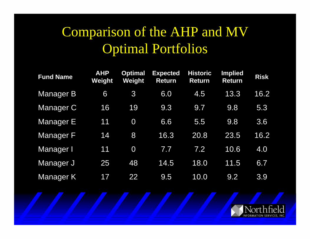
Comparison of the AHP and MV Optimal Portfolios

3.99.210.09.52217Manager K

6.711.518.014.54825Manager J

4.010.67.27.7011Manager I

16.223.520.816.3814Manager F

3.69.85.56.6011Manager E

5.39.89.79.31916Manager C

16.213.34.56.036Manager B

RiskImpliedReturn

HistoricReturn

ExpectedReturn

OptimalWeight

AHPWeightFund Name

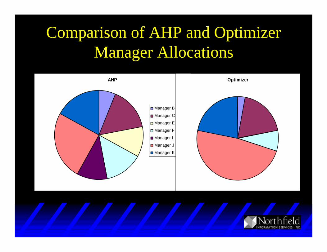
Comparison of AHP and Optimizer Manager Allocations

AHP

Manager B

Manager C

Manager E

Manager F

Manager I

Manager J

Manager K

Optimizer

Conclusions

u AHP is a methodology that arises from operations research literature that is used as a non-parametric method for making complex, often qualitative decisions in a robust, consistent fashion.

u AHP has now been adapted as a tool in the selection of, and the allocation of capital to, investment managers.

u We think AHP is the way to go for many problems in investment decision making where quantitative and qualitative criteria must both play a role.