Using Simulation Early in the Design of a Fuel Injector Production Line 

 u  M  stafa H. Tongarlak Bruce Ankenman     Barry L. Nelson     

North r ity      

western Unive s 

Laurent Borne   McKinsey & Company 

 Kyle Wolfe     

Del on phi Corporati 

July 27, 2009 

 

Abstract 

Delphi Corporation decided to use simulation from concept development to installation of  a  new multimillion  dollar  fuel  injector  production  line.  In  this  paper we  describe  how simulation was employed in the concept development phase to assess whether production targets  required  for  financial  viability were  feasible and  to  identify  the  critical  features of the line on which to focus design‐improvement efforts. 

1. Introduction 

Delphi Corporation  is a major  supplier of  fuel  injectors  to auto manufacturers around the world. The company  is considering a proposal for a new  line that will produce the next  generation  of  fuel  injectors.  There  are  ambitious  requirements  on  the  line’s throughput that are essential for the project to be financially viable, and real constraints on the space available for the line and the cost to build it and staff it.   

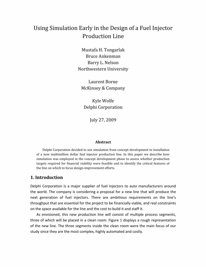
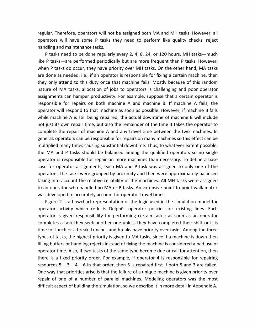
As envisioned,  this new production  line will  consist of multiple process  segments, three of which will be placed in a clean room. Figure 1 displays a rough representation of the new  line. The three segments  inside the clean room were the main focus of our study since they are the most complex, highly automated and costly.   

Cartridge Assembly

Injector Assembly

Calibration & Test

CLEAN ROOM

WHITE ROOM

Subassemblies

Injector

RAIL ASSEMBLY 

Figure 1. Proposed fuel injector production line. 

Each  process  segment  may  contain  as  many  as  thirty  machines  and  robots performing various tasks along accumulating conveyors that convey partially completed fuel injectors from machine to machine in pallets. The conveyors will also act as buffers since they accumulate pallets in front of a machine if it is either down or unable to keep up  with  the  flow  of  pallets  from  upstream  machines.  Transfer  of  assembled  fuel injectors between process segments will be done via trays that are stacked in carts and moved manually  by  operators.  Because  contamination  is  a major  concern  inside  the clean  room,  parts will  be washed  before  entering  the  clean  room  and  operators  are assigned tasks that do not require them to move between rooms.   

A simulation model and study was commissioned at a very early stage of designing the  new  line.  The  goal  for  the  simulation was  to  serve  as  a  test  bed  for  candidate production‐line designs, both from initial concept to fine tuning and even to examining process‐improvement ideas after the line is in place. To simulate a line design it must be fully  specified  including which machines  to use  and  in what order,  conveyor  lengths, machine process rates and variability, operator responsibilities and priorities, and failure and  repair  distributions  for  each machine,  as  well  as  scrap  and  rework  rates  on  a machine‐by‐machine  basis.  Such  complete  and  detailed  information  is  typically  not available at the concept stage of  the  line design, but  this  is precisely when simulation can be most valuable in helping Delphi to assess whether the project is financially viable and where in the evolving line design the most effort should be spent. Using simulation at  such  an  early  stage  requires  making  frequent  and  significant  changes  to  the simulation  base model  which  can  be  both  time‐consuming  and  difficult  to manage. However,  the  recommendations  from  the  study  are  often  inexpensive  or  free  to implement  since  the equipment has not  yet been built. Once  the equipment  is built, using simulation to analyze the process is less time‐consuming because the base model is not a moving  target. The drawback  to waiting, however,  is  that much of  the cost  is 

already  sunk  and  the  recommendations  from  the  study  may  be  more  difficult  to cost‐justify. This was our challenge.   

Notice that it makes no sense early on to try to optimize the design over the literally hundreds of  changeable  features because  too  little  is known and  too much  is  in  flux. Instead,  simulation  was  exploited  to  answer  high‐level  questions  about  the  line configuration,  with  the  understanding  that  the  model  would  later  evolve  into  a representation capable of evaluating very specific questions. That is, the simulation was first  to  guide  the  development  of  new  designs  by  distinguishing  critical  features  and factors from less‐critical ones, and later to be updated as new designs emerged. In this way  the  simulation would provide a perpetual  road map  for next  steps  in  the design process.  This  paper  is  a  product  of  the  first  phase  (about  6 months)  of  this  iterative design process where answering high‐level questions about line configuration, conveyor layout, and operator assignments was of primary concern. In this way we will illustrate how simulation can have a profound impact at the concept stage of a complex project.   

2. System Description and Data Sources 

Clearly machines (including robots) and conveyors need to be included in the simulation model. Most machines will keep  running until a  failure occurs as  long as  they are not starved or blocked. Since conveyors will be handling the subassemblies within process segments, operators are needed only for transferring assembled fuel injectors between process  segments,  filling  raw  material  buffers,  repairing  machines  and  periodically performing  other  tasks  such  as  quality  checks,  rejected  fuel  injector  handling  and preventative maintenance. Even  though  the  system  is  semi‐automated and operators are only  lightly  involved with actual operations,  their  supporting  role  in  the  system  is critical because machine failures will occur, and input buffers will be consumed, leading to lost production if operators are unable to keep up. Therefore, in addition to machines and conveyors, operators, injector trays and material carts were included in the model.   

Delphi  represented  line  designs  as  AutoCAD  drawings  (that  eventually  became backgrounds for the simulation animation). More importantly, Delphi also maintained a single Excel spreadsheet with many worksheets called the Manufacturing System Design (MSD) that always contained the current state of knowledge about the line design. This included process  information of all types,  from raw material buffer sizes and operator task  assignments  to  anticipated  machine  reliabilities,  processing  times  and processing‐time  variabilities.  Since  this  information  ranged  from  firm  values  and commitments  to  educated  guesses,  and  would  evolve  and  expand  throughout  the project, a  link was established between the MSD and the simulation model so that the simulation would always be run with the most up‐to‐date data.   

However, the MSD was more than just a data source; it was also used to balance the 

line to produce k fuel injectors every minute (where k was a value set by Delphi and will not be revealed here).  In this semi‐automated system where a series of processes are connected to each other, “balancing” simply means that if a particular operation is not able to produce the target k parts per minute then enough parallel capacity is added to keep up with the production requirement. Since the line will operate for 24 hours/day, the production capacity of the line would be 1440k parts/day if there were no machine downtimes, no scrap, no process variability and material buffers would never go empty. However,  to  bring  more  realism,  the  MSD  also  incorporated  discount  factors  for percentage of scrap and downtime by machine,  leading to a still optimistic throughput target of 1225k  fuel  injectors per day, or approximately 22%  less  than  the  theoretical maximum.  Achieving  this  target  is  necessary  for  the  new  fuel  injector  project  to  be financially viable.   

The  reason  that  1225k  fuel  injectors  per  day may  be  optimistic  is  that  a  static analysis, such as the MSD provides, cannot account for the impact of process variability, starvation  due  to  lack  of  material  or  blocking,  operator  response  time  to  failures, conveyor congestion, etc. More accurate analysis of the proposed system requires the fidelity of a detailed simulation model which  takes  into consideration  the  interactions among all parts of the system as well as randomness inherent to the system. The critical question to be answered by the simulation at the concept stage was whether 1225k fuel injectors per day was actually feasible and what it might take to get there.   

In the following subsections we list some of the key system elements that figured in our analysis and mention any approximations we made.   

2.1. Resources 

Each machine  is prone  to  failure and  the average  time  it  runs until a  failure occurs  is represented by a Mean Time Before Failure  (MTBF). Once  it  fails, a machine waits  for the appropriate operator to come and fix  it. The time  it takes for an operator to arrive and then repair the machine is downtime when no parts can be produced. The average repair time is denoted by Mean Time To Repair (MTTR). The MTBF and MTTR are values derived  from  information  in  the MSD, and  the distributions of  the  time  to  failure and repair were modeled as exponential. The exponential distribution was chosen because, in the absence of real data, it can be specified by a single parameter, and it reflects the high variability observed by Delphi in existing lines.   

2.2. Operators 

There  are  three  types  of  tasks  that  need  operators: Machine  Attention  (MA)  Tasks, Periodic  (P)  Tasks,  and Material  Handling  (MH)  Tasks.  Each  type  of  task  requires  a different set of skills. MA tasks have the highest variability while MH tasks are the most 

regular. Therefore, operators will not be assigned both MA and MH tasks. However, all operators  will  have  some  P  tasks  they  need  to  perform  like  quality  checks,  reject handling and maintenance tasks.   

P tasks need to be done regularly every 2, 4, 8, 24, or 120 hours. MH tasks—much like P tasks—are performed periodically but are more frequent than P tasks. However, when P tasks do occur, they have priority over MH tasks. On the other hand, MA tasks are done as needed; i.e., if an operator is responsible for fixing a certain machine, then they only attend  to  this duty once  that machine  fails. Mostly because of  this  random nature  of MA  tasks,  allocation  of  jobs  to  operators  is  challenging  and  poor  operator assignments can hamper productivity. For example, suppose that a certain operator  is responsible  for  repairs  on  both  machine  A  and  machine  B.  If  machine  A  fails,  the operator will respond to that machine as soon as possible. However,  if machine B fails while machine A  is still being repaired, the actual downtime of machine B will  include not just its own repair time, but also the remainder of the time it takes the operator to complete  the  repair of machine A and any  travel  time between  the  two machines.  In general, operators can be responsible for repairs on many machines so this effect can be multiplied many times causing substantial downtime. Thus, to whatever extent possible, the MA  and  P  tasks  should  be  balanced  among  the  qualified  operators  so  no  single operator  is responsible  for repair on more machines  than necessary. To define a base case  for operator  assignments, each MA  and P  task was  assigned  to only one of  the operators, the tasks were grouped by proximity and then were approximately balanced taking  into account the relative reliability of the machines. All MH tasks were assigned to an operator who handled no MA or P tasks. An extensive point‐to‐point walk matrix was developed to accurately account for operator travel times.   

Figure 2  is a flowchart representation of the  logic used  in the simulation model for operator  activity  which  reflects  Delphi’s  operator  policies  for  existing  lines.  Each operator  is  given  responsibility  for  performing  certain  tasks;  as  soon  as  an  operator completes a task they seek another one unless they have completed their shift or  it  is time for lunch or a break. Lunches and breaks have priority over tasks. Among the three types of tasks, the highest priority is given to MA tasks, since if a machine is down then filling buffers or handling rejects instead of fixing the machine is considered a bad use of operator time. Also, if two tasks of the same type become due or call for attention, then there  is  a  fixed  priority  order.  For  example,  if operator  4  is  responsible  for  repairing resources 5 – 3 – 4 – 6  in that order, then 5  is repaired first  if both 5 and 3 are failed. One way that priorities arise is that the failure of a unique machine is given priority over repair  of  one  of  a  number  of  parallel machines. Modeling  operators  was  the most difficult aspect of building the simulation, so we describe it in more detail in Appendix A. 

 

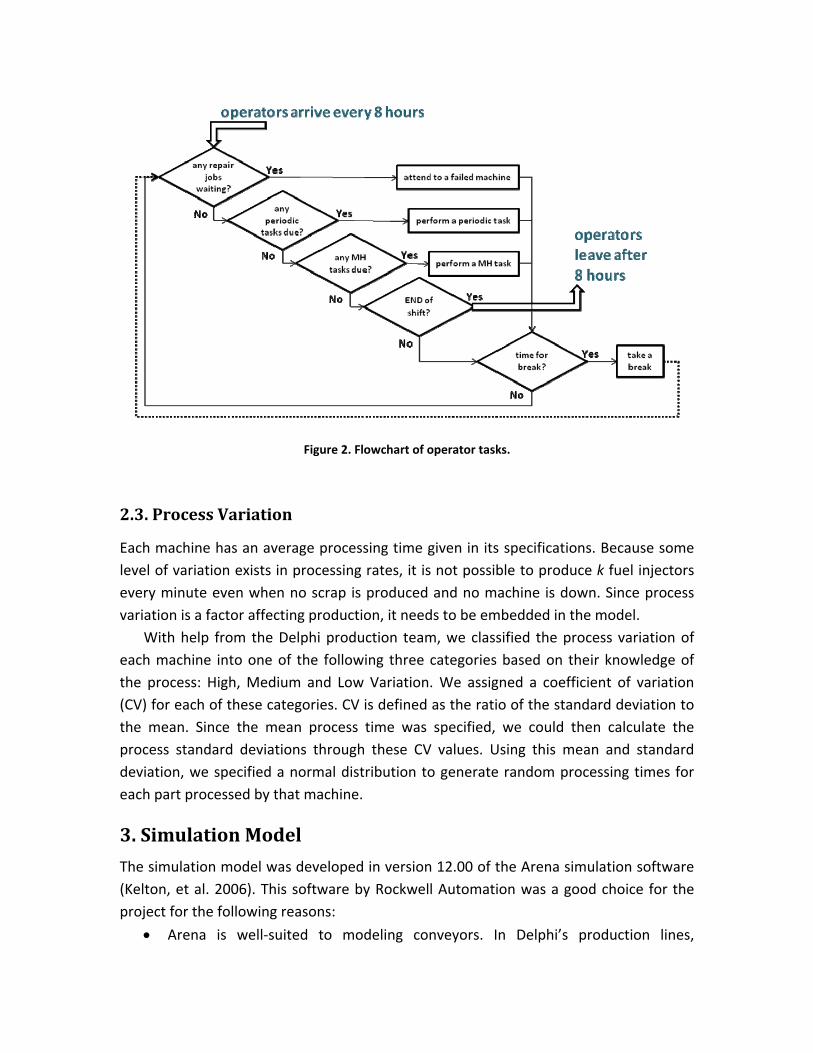
Figure 2. Flowchart of operator tasks. 

 

2.3. Process Variation 

Each machine has an average processing time given  in  its specifications. Because some level of variation exists in processing rates, it is not possible to produce k fuel injectors every minute even when no scrap  is produced and no machine  is down. Since process variation is a factor affecting production, it needs to be embedded in the model. 

With help  from  the Delphi production  team, we classified  the process variation of each machine  into one of  the  following  three categories based on  their knowledge of the process: High, Medium  and  Low Variation. We  assigned  a  coefficient of  variation (CV) for each of these categories. CV is defined as the ratio of the standard deviation to the mean.  Since  the mean  process  time was  specified, we  could  then  calculate  the process  standard  deviations  through  these  CV  values. Using  this mean  and  standard deviation, we specified a normal distribution to generate random processing times  for each part processed by that machine.   

3. Simulation Model 

The simulation model was developed in version 12.00 of the Arena simulation software (Kelton, et al. 2006). This software by Rockwell Automation was a good choice  for the project for the following reasons:   

• Arena  is  well‐suited  to  modeling  conveyors.  In  Delphi’s  production  lines, 

conveyors are the major mode of material transfer.   

• Arena  provides  a  user‐friendly  interface  that  makes  understanding  and modifying  the model easier  for people other  than  the modeler.  In  addition,  it gives the ability to design templates through which similar code can be created for  the  parts  of  the  model  that  are  likely  to  be  repeated  with  different parameters.  For  instance,  we  designed  a  template  that  handles  the  tasks performed when a part arrives to a machine to be processed, such as picking the part from the conveyor, checking for raw material inventory, processing the part and  placing  the  part  back  to  the  conveyor. Once  the  template  is  available,  a modeler only needs to define machine‐specific parameters  like conveyor name, machine  number,  buffer  type,  etc.  and  customized  code  will  be  generated automatically.   

• The model can be  linked to a data source (e.g., the MSD, an Excel spreadsheet) to  allow  for  making  most  minor  updates  (e.g.,  changing  MTBF  for  some machines)  directly  in  Excel  rather  than  in  Arena.  This  also  preserves  data integrity since all Delphi analyses use a common data source.   

• Arena provides animation capability  that can be used  for model validation and demonstration purposes.   

• Arena collects and reports most of the necessary statistics by default and lets the modeler add other statistics.   

4. Simulation Experiments and Results 

The main performance measure in our simulation study was long‐run average daily fuel injector  throughput;  i.e.,  the  long‐run  average  number  of  fuel  injectors  that  can  be produced  in a 24 hour period. Therefore, we  treated  this as a steady‐state simulation (Banks et al. 2005) requiring a so‐called “warm‐up period” to get from the  initial state (conveyors empty, but all  input buffers  full and all machines operational)  to  long‐run operating  conditions.  For  the  base  case  (described  below)  approximately  one  day’s production was adequate  (see Appendix B), so we made each replication 11 days  long with the output data from the first day discarded and 10 days (two weeks) retained. We then made enough replications to estimate  long‐run average throughput to within 5% relative  error,  and  this  required  20  replications.    (The  number  of  replications  was empirically determined  so  that  (Halfwidth of Confidence  Interval)/(Sample Mean) was less  than 0.05  for  the estimated  throughput.) To  give  some  idea of  the experimental effort to run one scenario, it takes approximately 8 hours to obtain 20 replications of 11 days on a  relatively  fast PC. This  is a  function of both  the  size and  complexity of  the system, and the very large number of fuel injector subassemblies in process at any one time.  Since all other  scenarios are modifications of  the base  case, we used  the  same 

experimental  effort  (20  replications  of  11  days)  on  each  of  the  scenarios  tested. Although  throughput  was  the  driving  performance  measure,  measures  of  operator utilization, machine  downtimes,  congestion  on  conveyor  segments,  and  raw material buffer states were also examined.   

Results  from  all  experiments were  compared  to  two  benchmarks:  the  base  case, which  is a simulation of Delphi’s  line design as specified  in the MSD; and the target of 1125k  fuel  injectors per day.  If  there had been no  gap between  these  two,  then  the proof‐of‐concept  phase  of  the  line  design would  be  done.  Instead,  there was  a  very substantial gap, so the objective became finding the key factors that produce the gap so that  they  can become  the  focus of  future design  efforts.  This must be done without specific  design  alternatives  with  which  to  compare,  which  led  to  the  experimental approach  described  below.  The  critical  factors  were  unexpected,  but  completely understandable after the fact.   

4.1. First­Phase Scenarios 

To design our preliminary experiments, called “first‐phase scenarios,” we listed all of the factors  that may  contribute  to  the  loss  of  production.  Obviously,  if  no  such  factors existed,  then we would  be  consistently  producing  1125k  fuel  injectors  per  day.  The following  are  some  of  the  factors we  listed  as  potentially  critical:  Process  variability, scrap rates and downtime related to operator availability. Secondary  factors we  listed included  conveyor  lengths  and number of pallets on  each  conveyor. We  focused our initial  experimentation  on  the  potentially  critical  factors  because  we  felt  that conclusions about  conveyors would be premature at  this  stage of  the  study  since big changes to the line layout were very likely. 

In the simulation, downtime could be controlled by manipulating the machine repair time. Since there are 25 machines, and since each machine has a specified scrap rate, process  variability  and  repair  time,  there  are  75  factors  that  could  be  analyzed with classical design‐of‐experiments methods. However, even  if we prioritized and selected only 30 of these 75 factors, and examined just the main effects, at least 32 runs would be required. At 8 hours per test plus the time spent setting up scenarios and analyzing results,  this  experiment would  take  about  2 weeks. At  the  concept  stage  of  the  line design  investing 2 weeks of  time and  computational effort  to estimate  the effects of each individual factor is not worthwhile since many details are in flux and major changes to  equipment  and  conveyor  layouts  are  almost  certain.  Therefore, we  used  a  group screening approach, grouping the factors into functional categories. By categorizing the impact or  lack of  impact of  these  functional groups we could answer broad questions about which factors have the greatest impact with reasonable computing effort.   

For instance, instead of investigating each machine’s process variability individually, 

we  investigated  the  effect  of  eliminating  all  the  process  variability;  this  allows  us  to quantify the maximum impact that process variability has on throughput and saves the effort required to assess the effect of process variability for each of the 25 machines if it turns  out  that  process  variability  as  a  group  is  not  very  significant. We  constructed analogous scenarios to examine the group effects of scrap rates and repair times. Thus, the first‐phase scenarios included:   

• Scenario 1: Base case, the model representation of the factory as reflected in the MSD file and the AutoCAD drawing of the layout.   

• Scenario 2: All process variation is removed from the base case.   

• Scenario 3: Process variation and all scrap are eliminated from the base case.   

• Scenario 4: Repair times are set to zero; that  is, as soon as an operator attends to a failed machine,  it starts running again and the operator can  leave for their next assignment.   

 Scenario 2, which eliminates  the process  variation, was especially  critical because 

the  variation  input  to  the model was  based  on  expert  opinion  and  estimated  CV’s. Therefore, if eliminating all the variation does not achieve a significant production gain, then putting effort into creating better estimates of CV for the processing time of each machine is not essential at the conceptual design stage. If, on the other hand, it makes a significant  difference,  then  we  should  not  make  radical  design  changes  before  this variation is carefully characterized. 

Scenario 3 eliminates both scrap and process variation. This scenario was  intended to  inform  us  of  the  sensitivity  of  throughput  to  scrap  rates  and  to  determine  if  it  is critical  to  improve  the  estimates  of  the machine  scrap  rates  before  proceeding.  The purpose  of  eliminating  both  process  variation  and  scrap  rate  together  is  to  use  this scenario as a “best case scenario" for this design candidate.   

Scenario 4 takes a different approach than 2 and 3. In this experiment, repair times were set to zero while scrap and process variation were retained. The goal was to see the potential of the production  line when repairs are done infinitely fast and machines are down only for the amount of time it takes for the designated operator to attend the machine (i.e., response time, which consists of time to complete a task in progress and walking  travel  time). When  repair  times  were  set  to  zero,  operators  become more available and as a result response times to failures also decrease. We recognize that this level  of  service  is  impossible  to  achieve  but  this  scenario  showed  us  the  benefits  of improving machine attention activities.   

4.2. First­Phase Results and Analysis 

For the base case scenario, the average daily production value estimate was only 800k 

fuel injectors per day or 71% of the target throughput for the new line. This left a gap of nearly 30% between planned and realized production. The results of scenarios 2–4 shed light  on  what  caused  this  gap  and  what  design  changes  would  give  the  largest improvement. 

In scenario 2 when process variation was taken out from all of the machines, daily production  relative  to  the goal went up  to 75%.  In  scenario 3,  in which both process variability  and  scrap  were  eliminated,  this  percentage  became  76%.  Both  of  these drastic  and  unattainable  changes  to  the  system  produced  only  slight  increases  in productivity. Therefore, we concluded  that more detailed analysis of machine process variation and  scrap  rates  should be  left  to  later  stages of our  study after other more influential changes were made to the system.   

In  scenario  4,  in which  repair  times  are  reduced  to  zero,  the  goal  of  1125k  fuel injectors per minute was achieved. In fact the average daily production for this scenario was 102% of the target. This significant jump from base case was a good indication that machine downtime is one of the primary causes of the low production in the base case. However, before we  jumped to a conclusion too quickly, we returned to the base case scenario and  looked at statistics that were collected to discover other reasons  for  lost production. There were four types of analysis we were  interested  in making: Operator availability, pallet congestion, inventory levels, and failure analysis.   

Operator  utilizations  in  the  base  case  showed  all  operators were  heavily  utilized. Some  operators were  so  very  heavily  utilized  that  they  often  did  not  complete  their periodic tasks, such as quality checks, during their shift and so these tasks were pushed to the following shift. For certain tasks, the operators in subsequent shifts were also too busy to complete these tasks and thus it was clear that these types of jobs would build up and never be  completed. An even more  significant  consequence of having heavily utilized operators  is that many machine  failures did not get  immediate attention  from operators  and  thus  operator  response  time  to machine  failure  began  to  overwhelm repair  time  as  the  primary  cause  of  machine  downtime.  This  raised  the  machine downtimes  for most machines far above the expected downtime and caused dramatic production losses.   

Another system measure is congestion on conveyors. A very straightforward way of knowing which  conveyor  segments  experience  higher  congestion  is  to  look  at which segments are heavily utilized  for a  long  time. Before running any of  the scenarios, we created 4 utilization  states:  Fully, Highly, Moderately and  Lightly Utilized. Throughout the 10 days of each replication, we monitored the amount of time that each conveyor segment  spent  in  each  utilization  state.  Conveyor  segments  that  spent  a  high percentage of time in Fully or Highly Utilized states were marked and compared to the machine downtimes in the vicinity of these conveyors. Our conclusion for the base case 

was that there is a very strong relationship between operators not being able to quickly respond  to  machine  failures  and  heavy  utilization  of  the  conveyor  segments  just upstream of those machines.   

Raw material buffer inventory is also of interest. The question is whether there are machines  that  go  idle  due  to  lack of material.  In  all  of  our  scenarios,  there was  one operator dedicated to raw material handling and that operator had no machine repair responsibilities.  Thus,  this  function  was  not  affected  by  the  excessive  machine downtime.  Our  conclusion  from  analyzing  inventory  buffers  was  that  the  material handling assignments  for  the base case worked out very well and needed only minor adjustments.   

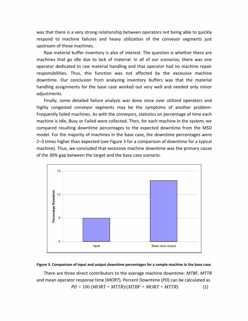
Finally,  some  detailed  failure  analysis was  done  since  over  utilized  operators  and highly  congested  conveyor  segments  may  be  the  symptoms  of  another  problem: Frequently failed machines. As with the conveyors, statistics on percentage of time each machine is Idle, Busy or Failed were collected. Then, for each machine in the system, we compared  resulting downtime percentages  to  the  expected downtime  from  the MSD model. For the majority of machines in the base case, the downtime percentages were 2–3 times higher than expected (see Figure 3 for a comparison of downtime for a typical machine). Thus, we concluded that excessive machine downtime was the primary cause of the 30% gap between the target and the base case scenario.   

Figure 3. Comparison of input and output downtime percentages for a sample machine in the base case. 

There are three direct contributors to the average machine downtime: MTBF, MTTR and mean operator response time (MORT). Percent Downtime (PD) can be calculated as   

PD = 100 (MORT + MTTR)/(MTBF + MORT + MTTR)  (1) 

Percent machine  downtime  for  the MSD model was  estimated  by  observing  current machines that are similar to the ones planned  for the new production  line. Because  it directly affects the production, percent downtime for each machine  is often recorded. MTBF  for  the MSD model  is also easily  collected  since machines often have  runtime monitors on them. However, separating out the operator response time from the repair time  is not  typically done,  and would  in  fact be  very difficult without  a  lengthy  time study on each machine. This means that we can easily estimate the sum of MORT and MTTR, but we cannot estimate either of  them  individually. When setting up  the base case scenario, this problem came into play since each machine must have a distribution specified for both time before failure (TBF) and time to repair (TTR). As a simplification, we  assumed  that  if  operator  assignments were well  designed  then MORT would  be substantially less than MTTR and thus negligible. Therefore, solving (1) for MTTR we get    

  ( )/ 100MTTR PD MTBF PD≈ × −   (2) 

where  PD   and  MTBF   are  the estimates of percent machine downtime  and MTBF from the MSD. Given the results of scenario 4, the assumption that MORT  is negligible was incorrect for the base case and the approximation for MTTR in (2) is poor.   

The first response to this information is that all reasonable effort should be made to determine  a  good  estimate  of MTTR  for  each machine  so  that  the  base  case  can  be correctly  simulated.  However,  this would  require  substantial  time  to  carry  out  data collection at a current production facility with similar machines, if they could be found. Another option, more in the spirit of the use of simulation early in the design process, is to  redesign  the base case  to  reduce  the operator  load and  thus  reduce  the  impact of MORT. Additional scenarios were used to help to understand the problem of operator loading on the base case and potentially suggest new design directions.   

4.3. Second­Phase Scenarios 

In light of the results of first‐phase scenarios, the second‐phase experiments focused on operator availability  for machine  failures. The operator assignments  for  the base case scenario  involved  some  critical  assumptions,  some  of which may  have  a  substantial impact on daily production numbers. For instance, in the base case design, each task (a quality check, a machine  repair or a material handling  job) was assigned  to a  specific operator and no other operator on  that  shift  could  respond  to  that  task. As a  result, when a particular operator was heavily utilized,  failed machines would often wait  for long periods of time before the assigned operator would arrive to start repairs. Similarly, when an operator was gone for their lunch or break, any failed machine assigned to that 

operator would have to wait until the  lunch or break was completed before any repair began. In this highly connected production system, any deviation of a machine from its production target is enough to slow down finished fuel injector throughput. 

Another assumption in the base case was that operators leave for lunch or break on schedule as soon as the task at hand  is completed. In some cases, this could  leave one or more machines failed through an entire lunch or break period. In addition, all of the operators go  to  lunch or break at  the  same  time,  further  complicating  the downtime problem. Clearly  the  throughput  gap might be  reduced by  redesigning  the  lunch  and break times of operators, possibly cross‐training some operators to provide back‐up for others, or by setting  the priorities differently  regarding  lunches and breaks or specific machines.   

To quantify  the potential of operator redesign, Scenario 5 used  the base case, but eliminated lunches and breaks from operator schedules. This experiment was designed to  determine  an  upper  bound  on  the  production  gain  that  could  be  achieved  by optimizing the rules on operator lunches and breaks, while the base case implemented a worst‐case scenario where lunch and breaks not only have priority, but also all occur at the same  time. Of course working operators without any breaks  is not realistic, nor  is having them all take lunch at the same time. However, the point of these experiments is not  to make  a  final  suggestion  for  implementation,  but  instead  to  guide  the  design efforts.  Furthermore,  there  are practical ways  to  implement  coverage of  lunches and breaks,  such  as  adding  support  operators  to  relieve  operators  when  they  leave  for breaks so all the tasks are continually done.   

The selection of scenario 6 was intended to determine how much the approximation of MTTR in (2) affected the daily production rate in the base case. Recall that MTTR for each machine  is  a  direct  input  to  the  simulation model. More  specifically,  each  time machine j failed, a random repair time was drawn from an exponential distribution with 

mean,  jMTTR , which was  calculated  from  (2)  using  estimates  of  the  downtime  and 

MTBF  for  that  machine  or  comparable  machines  from  current  production  lines. Operator  response  time, on  the other hand,  is  a  random output  from  the  simulation model which depends on the random machine failures as well as the operator utilization levels. The approximation in (2) used for the base case assumes that all of the downtime is repair time and we found this to be inaccurate. Scenario 4 went to the other extreme and assumed that all the downtime was operator response time, which we also know is not true since repairs do take time. Scenario 6 attempts to split the difference between these  two  scenarios  and  assumes  that  the  repair will  account  for  about  half  of  the downtime and operator response time will be the other half. Thus, for scenario 6, the MTTR for each machine was cut in half. Therefore, the following two scenarios were run as second‐phase scenarios:   

• Scenario 5: Full relief of  lunch and breaks. This scenario has  lunches and breaks fully staffed with no reduced efficiency.   

• Scenario 6: Mean  time to repair  (MTTR)  is cut  in half. This scenario anticipates that about half of the machine downtime is operator response time.   

In both of these scenarios, the base case assumptions are kept the same except for the  changes mentioned.  Thus,  scrap  and  process  variability  rates  are  included  at  the same levels as in the base case.   

4.4. Second­Phase Results 

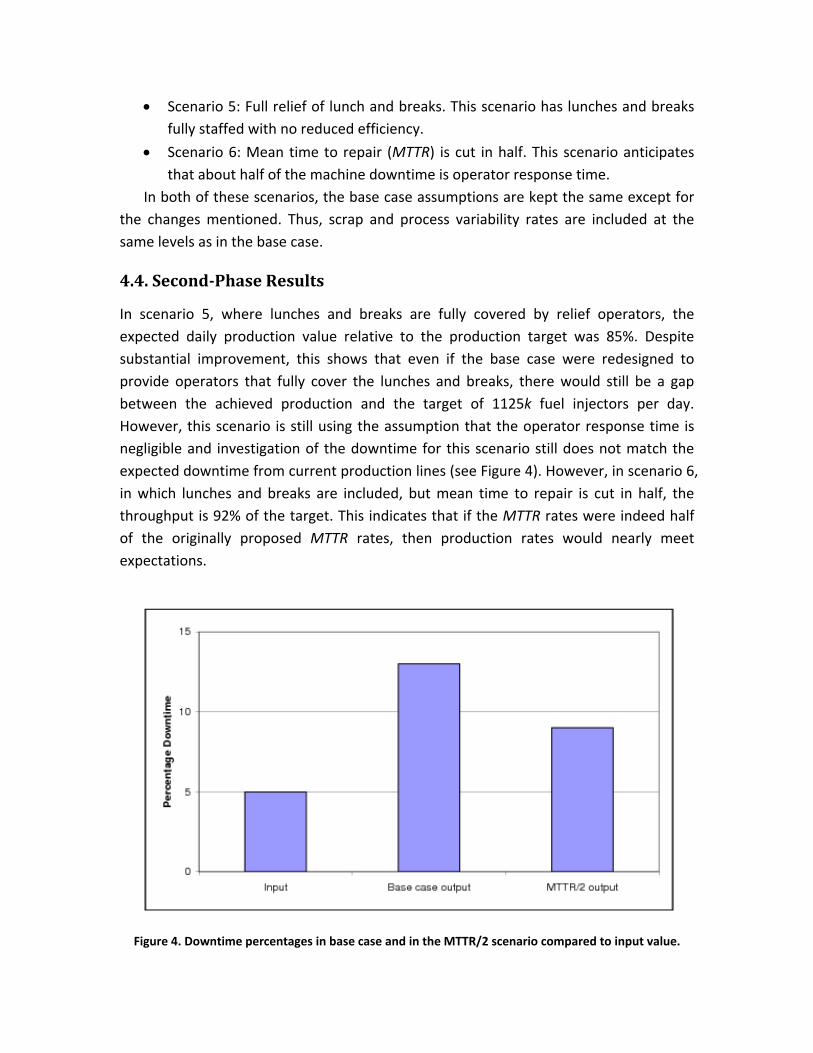
In  scenario  5,  where  lunches  and  breaks  are  fully  covered  by  relief  operators,  the expected  daily  production  value  relative  to  the  production  target was  85%.  Despite substantial  improvement,  this  shows  that  even  if  the  base  case were  redesigned  to provide operators  that  fully  cover  the  lunches and breaks,  there would  still be  a gap between  the  achieved  production  and  the  target  of  1125k  fuel  injectors  per  day. However, this scenario  is still using the assumption that the operator response time  is negligible and  investigation of the downtime  for this scenario still does not match the expected downtime from current production lines (see Figure 4). However, in scenario 6, in which  lunches and breaks are  included, but mean  time  to  repair  is  cut  in half,  the throughput  is 92% of the target. This indicates that  if the MTTR rates were  indeed half of  the  originally  proposed  MTTR  rates,  then  production  rates  would  nearly  meet expectations.    

Figure 4. Downtime percentages in base case and in the MTTR/2 scenario compared to input value. 

Caution must be taken in interpreting scenario 6. The operator response time in the simulation model is based on the level of operator staffing and their assignments. Recall that the downtime estimates from current production machines are also based on some level of operator  staffing and  some  system of  task assignment  that was not  recorded (and are not necessarily  relevant  to  the new production  line). Thus,  the conclusion of this second phase is that it is vitally important to determine an accurate estimate of the MTTR  for each machine that  is  independent of the operator response time. Only with good  estimates  of MTTR  can  accurate  estimates  of  the  daily  throughput  be  trusted. Once  accurate  estimates  of  the MTTR  for  each  machine  are  collected,  new  design candidates can be accurately tested.  In particular, scenario 5  indicated that substantial increases  in daily throughput can be gained by working out an operator schedule that provides task coverage for operators when they take lunch or breaks.   

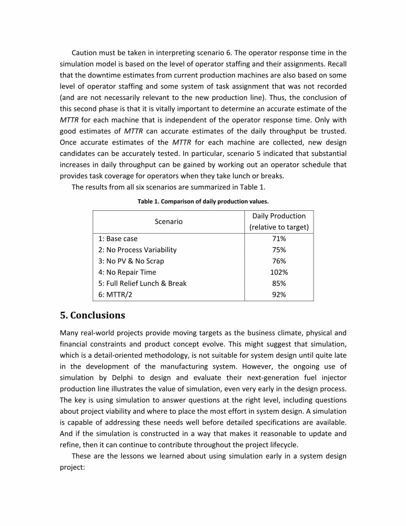
The results from all six scenarios are summarized in Table 1.   

Table 1. Comparison of daily production values. 

Scenario Daily Production (relative to target) 

1: Base case  71% 2: No Process Variability 75% 3: No PV & No Scrap 76% 4: No Repair Time  102% 5: Full Relief Lunch & Break 85% 6: MTTR/2  92% 

5. Conclusions 

Many real‐world projects provide moving targets as the business climate, physical and financial  constraints  and  product  concept  evolve.  This might  suggest  that  simulation, which is a detail‐oriented methodology, is not suitable for system design until quite late in  the  development  of  the  manufacturing  system.  However,  the  ongoing  use  of simulation  by  Delphi  to  design  and  evaluate  their  next‐generation  fuel  injector production line illustrates the value of simulation, even very early in the design process. The key  is using simulation  to answer questions at  the  right  level,  including questions about project viability and where to place the most effort in system design. A simulation is  capable of addressing  these needs well before detailed  specifications are available. And  if  the  simulation  is constructed  in a way  that makes  it  reasonable  to update and refine, then it can continue to contribute throughout the project lifecycle.   

These are  the  lessons we  learned about using  simulation early  in a  system design project:   

• The simulation model should be constructed so that it is easily changed. Ideally it should be  linked  to  the  same data  sources  that are being used  for  the overall project planning.   

• Group screening should be used to assess which design features or data sources, taken  together,  impact  performance  so  that  as  the  project  evolves  scarce engineering effort can be concentrated where it is most useful.   

• The temptation to create or define detailed production control plans should be avoided,  and  instead  easy‐to‐define,  extreme  scenarios  that  bound  potential improvements or effectiveness should be used.   

• Focus  not  only  on  the  output  performance measures  of most  interest  (e.g., throughput  here),  but  also  record measures  that  provide  insight  into  where problems might be occurring.   

6. Epilogue 

Upon  completion  of  the  first  6  months  of  the  concept  development  phase,  we presented the results and our conclusions to Delphi engineers and managers, including a manager  from Europe who was visiting  the plant at  the  time. This was  the  first major manufacturing  simulation  project  for  the Delphi  Powertrain  division  in  10  years. Our presentation generated a  lot of  feedback and sparked  interest  in carrying  forward  the simulation  study  for  another  three  months.  Taking  the  feedback  into  account,  we designed the next phase as a refinement of the concept development phase.   

Our  first  task was  to carefully calibrate downtimes  to set MTTRs, paying particular attention to machines with the  largest downtimes. Then, we experimented with three alternative coverage options  for operators: 1) Full  relief  (operators continuously work without  any  breaks);  2)  no  relief  (operators  take  periodic  breaks  during which  their responsibilities  await  their  arrival);  and  3)  staggered  breaks  with  cover  (operators working  in  the  same area never overlap  their breaks  so  that  they  can  cover  for each other). Among the three, only option 1 adds employees to cover for breaks. Options 2 and 3 require no additional resources and our results favored option 3 as the base case moving forward.   

After setting the base case, we then moved on to improving conveyor layouts. Based on a congestion analysis of conveyors, we  listed segments that were highly congested and could benefit from lengthening. We added to this list those segments that are very long and might add unnecessary travel time and take up space. We defined three levels (long, medium  and  short  length)  for  all  the  segments  in  the  list  and  ran  a  fractional factorial design to find the optimal  level for each segment. This analysis showed which segments  could  significantly  enhance  throughput  by  being  lengthened  or  shortened, and identified segments to which throughput was insensitive to their lengths.   

New  conveyor  layouts  were  constructed  based  on  the  suggested  sizing  of  the conveyor  segments.  One  of  the  conveyor  layouts  resulted  in  a  7%  improvement  in throughput compared to the current layout and a 10% reduction in required floorspace for no additional  investment. This layout was embraced by the Delphi team as a viable alternative to their original proposal. Finally, a pallet study showed that throughput was insensitive to the number of pallets within a very wide range.   

Insights gained by this simulation study convinced Delphi to continue to update the model as the equipment design evolves. In addition, impressed by the positive results of this project, Delphi management plans to use simulation on future programs.   

Acknowledgment 

Portions of this paper were published in the Proceedings of the 2008 Winter Simulation Conference, S.  J. Mason, R. R. Hill, L. Moench, O. Rose, eds. We thank the editors and referees for helpful guidance.   

References 

J. Banks, J. S. Carson, B. L. Nelson and D. Nicol. 2005. Discrete‐Event System Simulation. Fourth Edition. Prentice Hall, Inc., Upper Saddle River, NJ.   

W. D. Kelton, R. P.  Sadowski and D. T.  Sturrock. 2006.  Simulation with Arena.  Fourth Edition. McGraw‐Hill, New York.   

A. Modeling Operator “Bus Routes” 

Within Delphi, operator work assignments, as  illustrated  in Figure 2, are referred to as “bus  routes.”  The  name  was  derived  from  the  observation  that  operators  have sequences of repetitive tasks that they perform on certain cycles. However, unlike the typical  city  bus,  deviations  from  the  fixed  route  occur  due  to,  for  instance, machine failures  that  demand  immediate  attention,  after  which  the  route  can  resume.  This appendix  describes  how we  used  certain  features  of  Arena  to  simulate  the  complex work assignments of operators, and in particular their interaction with failed machines.   

In  a  typical  Arena  simulation,  operators  and machines  are  represented  by  Arena Resources. A Resource in Arena is, effectively, a variable that keeps track of the status of the operator or the machine it represents. When represented as Resources, a machine becomes unavailable when processing a job or when it is failed; similarly, an operator is considered unavailable when performing a task or on a break. This logic for Resources is usually  sufficient  for modeling machines with dedicated  repair  staff  that are  ready  to start fixing problems as soon as they occur, or for modeling a pool of operators whose only responsibility  is to respond to failures of a group of machines. Often the machine and operator Resource are one to one.   

However, this approach  is  inadequate for modeling the more complex scenario we faced where operators have a  variety of duties and machines with  failures must  stay unavailable  while  waiting  for  operator  attention.  The  machines  we  modeled  are semi‐automatic and therefore do not have dedicated operator support. The operators in the  system  have  duties  of  various  types,  ranging  from  machine  attention  tasks  to material handling and quality  checks  that make  representing  them with  the  standard Arena Resources inappropriate. Therefore, we used the flexibility of Arena to implement a custom approach.   

To  represent  the  operators  in  the  model,  an  Arena  Entity  is  created  for  each operator at the beginning of each shift, and is disposed at the end of the shift. As shown in Figure 2, operator Entities follow a routine in which they perform certain tasks in the priority order assigned to them. As opposed to the passive involvement of operators as Resources  that  are used by  Entities, here operators  are  actively  involved  in  choosing their  next  task  as  soon  as  they  become  available.  Repair  jobs,  periodic  tasks  and material handling tasks are created  in other parts of the model and operators respond to them at their earliest opportunity according to the priority of the tasks.   

We did  represent machines  as Resources, but we  chose not  to utilize  the built‐in failure  logic  of  the  Arena  Resources  because  it  does  not  allow  the  time  a machine spends waiting for an operator to depend on the current state of the operators. Instead, we established 3 states for each Resource, namely busy,  idle and failed,  idle being the 

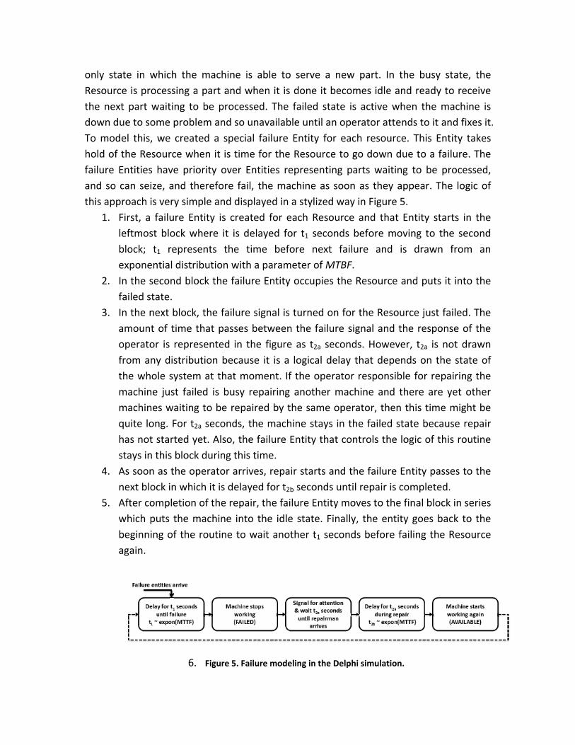
only  state  in which  the machine  is  able  to  serve  a  new  part.  In  the  busy  state,  the Resource is processing a part and when  it  is done  it becomes  idle and ready to receive the next part waiting  to be processed. The  failed  state  is active when  the machine  is down due to some problem and so unavailable until an operator attends to it and fixes it. To model  this, we  created a  special  failure Entity  for each  resource. This Entity  takes hold of the Resource when it is time for the Resource to go down due to a failure. The failure Entities have priority over Entities  representing parts waiting  to be processed, and so can seize, and  therefore  fail,  the machine as soon as  they appear. The  logic of this approach is very simple and displayed in a stylized way in Figure 5.   

1. First, a  failure Entity  is created  for each Resource and  that Entity  starts  in  the leftmost block where  it  is delayed  for  t1  seconds before moving  to  the  second block;  t1  represents  the  time  before  next  failure  and  is  drawn  from  an exponential distribution with a parameter of MTBF.   

2. In the second block the failure Entity occupies the Resource and puts it into the failed state.   

3. In the next block, the failure signal is turned on for the Resource just failed. The amount of time that passes between the failure signal and the response of the operator  is  represented  in  the  figure as  t2a seconds. However,  t2a  is not drawn from any distribution because  it  is a  logical delay  that depends on  the state of the whole system at that moment.  If the operator responsible for repairing the machine  just  failed  is busy  repairing another machine and  there are yet other machines waiting to be repaired by the same operator, then this time might be quite  long. For t2a seconds, the machine stays  in the failed state because repair has not started yet. Also, the failure Entity that controls the logic of this routine stays in this block during this time.   

4. As soon as the operator arrives, repair starts and the failure Entity passes to the next block in which it is delayed for t2b seconds until repair is completed.   

5. After completion of the repair, the failure Entity moves to the final block in series which puts  the machine  into  the  idle state. Finally,  the entity goes back  to  the beginning of the routine to wait another t1 seconds before failing the Resource again.    

6. Figure 5. Failure modeling in the Delphi simulation. 

B. Warmup Analysis 

A  practical  and widely  used method  for  finding  a  good warmup  period  is mean  plot analysis  (Banks,  et  al.  2005).  The  idea  is  simple:  Estimate  the  transient mean  of  the process by averaging across a number of replications then choose as the deletion point a  time after which  the plot  varies  consistently around a  fixed  value. Here we explain how we used this method in our fuel injector simulation.   

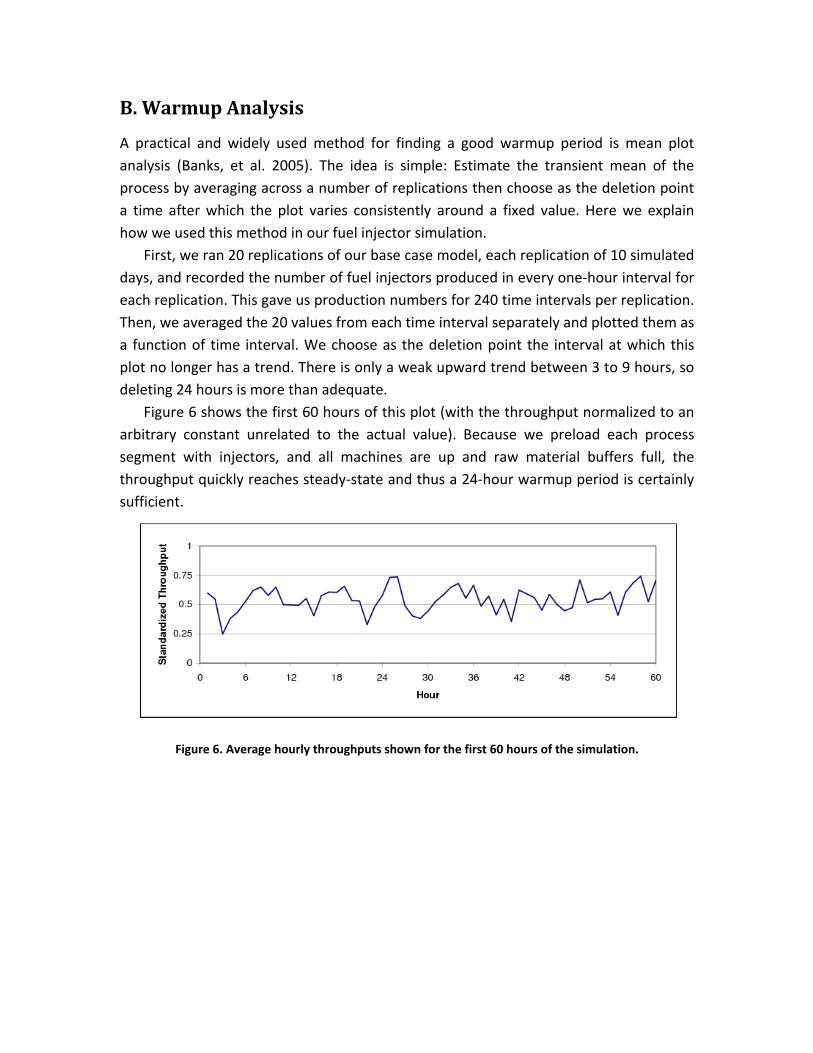
First, we ran 20 replications of our base case model, each replication of 10 simulated days, and recorded the number of fuel injectors produced in every one‐hour interval for each replication. This gave us production numbers for 240 time intervals per replication. Then, we averaged the 20 values from each time interval separately and plotted them as a  function of time  interval. We choose as the deletion point the  interval at which this plot no longer has a trend. There is only a weak upward trend between 3 to 9 hours, so deleting 24 hours is more than adequate.   

Figure 6 shows the first 60 hours of this plot (with the throughput normalized to an arbitrary  constant  unrelated  to  the  actual  value).  Because we  preload  each  process segment  with  injectors,  and  all machines  are  up  and  raw material  buffers  full,  the throughput quickly reaches steady‐state and thus a 24‐hour warmup period is certainly sufficient.   

Figure 6. Average hourly throughputs shown for the first 60 hours of the simulation.