using simbritain to model the geographical impact of ... · using simbritain to model the...
TRANSCRIPT

This is an author produced version of a paper published as Ballas, D., Clarke, G. P., Dorling, D. and Rossiter, D. (2007).
Using SimBritain to Model the Geographical Impact of National Government Policies. Geographical Analysis 39(1), 44-
77. This paper has been peer-reviewed but does not contain final published proof-corrections or journal pagination.
1
Using SimBritain to model the geographical impact of national
government policies
Dimitris Ballas|, Graham Clarke*, Danny Dorling
| and David Rossiter*
| Department of Geography, University of Sheffield, Winter Street, Sheffield S10 2TN, England
e-mail: [email protected]; [email protected]
* School of Geography, University of Leeds, Leeds LS2 9JT, England
e-mail: [email protected]; D.J.Rossiter @geog.leeds.ac.uk;
Abstract: In this paper we use a dynamic spatial microsimulation model of Britain for
the analysis of the geographical impact of policies that have been implemented in Britain
in the last 10 years. In particular, we show how spatial microsimulation can be used to
estimate the geographical and socio-economic impact of the following policy
developments: introduction of the minimum wage, winter fuel payments, working
families tax credits and new child and working credits. This analysis is carried out with
the use of the SimBritain, which is a product of a 3-year research project aimed at
dynamically simulating urban and regional populations in Britain. SimBritain projections
are based on a method that uses small area data from past Censuses of the British
population in order to estimate small area data for 2001, 2011 and 2021.
Keywords: spatial microsimulation, geographical impact analysis of national policies,
spatial forecasting
1. Introduction
This paper reports progress on SimBritain, which is an on-going research project that
aims at simulating a detailed social survey of households in Britain. The SimBritain
project brings together data from various public sector sources to develop and validate a
microsimulation model of the life of households in Britain from 1991 to 2021.
Microsimulation can be defined as a methodology that is concerned with the creation of
large-scale simulated population microdata sets for the analysis of policy impacts at the
micro-level. In particular, microsimulation methods aim to examine changes in the life of
individuals within households and to analyse the impact of government policy changes
for each simulated individual and each household. Microsimulation methodologies have
become accepted tools in the evaluation of economic and social policy and in the analysis
of tax-benefit options and in other areas of public policy (Hancock and Sutherland,
1992). Nevertheless, there are relatively few examples of spatial models that build on
traditional economic microsimulation frameworks by adding a geographical dimension.
Geographical microsimulation techniques involve the merging of census and survey data
to simulate a population of individuals within households (for different geographical
units), whose characteristics are as close to the real population as it is possible to estimate
(Williamson et al., 1998; Ballas, 2001; Clarke, 1996). Dynamic micro-simulation
involves forecasting key socio-economic variables into the future based either on current
trends or the consequences of different policy scenarios.
This is an author produced version of a paper published as Ballas, D., Clarke, G. P., Dorling, D. and Rossiter, D. (2007).
Using SimBritain to Model the Geographical Impact of National Government Policies. Geographical Analysis 39(1), 44-
77. This paper has been peer-reviewed but does not contain final published proof-corrections or journal pagination.
2
One of the main objectives of the research presented in this paper is to suggest a tool that
can be used to hold governments to account in terms of their long-term goals. It should be
noted that the SimBritain model is based on an initial simulation of the city of York, UK
which was used as a base to build a national model. In this paper we give examples of the
microsimulation results by showing some results on the city of York and how it has been
changing during the 1990s and how it can be expected to change over the next twenty
years. Further, we use the model to explore several aspects of life within each of these
household groups throughout the simulation period and attempt to identify the main
future determinants of poverty. We also examine the importance of various sources of
income for different household classes. York was chosen as the initial study city because
it was the base of Seebohm Rowntree‟s (2000) initial studies of poverty in Britain
roughly a century ago and is now a fairly typical English city.
Thus, the overall aim of the paper is to describe the construction of a model which has the
potential to be useful for spatial forecasting. As Ballas et al., (2005a) suggest, in socio-
economic terms, some variables are easier to forecast than others. Simulating future
ageing, births and deaths is perhaps the most straightforward. However. many other
socio-economic variables are more difficult to predict. A starting point is to argue that
current trends are likely to continue (at least in the short term). This allows the setting of
a baseline scenario. Then, alternative scenarios can be explored given policies that are
designed to change the direction of current trends. This is the type of what-if analysis
explored in the latter stages of this paper.
The rest of the paper is set out as follows. In section 2 we explore the ideas behind spatial
microsimulation and this form of socio-economic forecasting. In section 3 we describe
the SimBritain model from a technical perspective. The techniques for undertaking the
baseline scenarios are described in section 4 whilst results of various what-if analyses are
presented in section 5. In section 6 we explicitly examine small-area results using the
city of York. Concluding comments are offered in section 7.
2. Spatial microsimulation: conceptual and scientific issues
One of the main distinctions, which is rarely noted in the microsimulation literature, is
that between spatial and aspatial microsimulation. Microsimulation has a long history in
economics which led to the acceptance of the microsimulation method as a standard tool
for the evaluation of economic and social policy and in the analysis of tax-benefit options
and in other areas of public policy (Falkingham and Lessof, 1992; Hancock and
Sutherland, 1992; Harding, 1996; Milton et al., 2000; Sutherland and Piachaud, 2001).
The standard non-geographical microsimulation models have been built on a very good
basis that was formed during the course of systematic research by economists in the last
forty years. However, during that period geography has been persistently ignored by
microsimulation researchers and there are several reasons for this:

This is an author produced version of a paper published as Ballas, D., Clarke, G. P., Dorling, D. and Rossiter, D. (2007).
Using SimBritain to Model the Geographical Impact of National Government Policies. Geographical Analysis 39(1), 44-
77. This paper has been peer-reviewed but does not contain final published proof-corrections or journal pagination.
3
Lack of good quality geographical data: there were very few sources of
geographical socio-economic data. Even today there are no small area population
microdata, which is the standard datasets used by economic microsimulation
models
Computational intensity: the incorporation of geography into standard
microsimulation models increases significantly the computational demand
Concerns with simulation accuracy
Belief that geography is not important
Unfamiliarity with geographical data and methods
Some of these problems have been recently tackled due to an accelerating growth in the
volume, variety, power and sophistication of the computer-based tools and methods
available to support urban and regional analysis and policy-making. Developments in
hardware and software systems have enabled significant advances to be made in the
storage, retrieval, processing and presentation of spatially referenced data. There has also
been significant progress in the development of Geographical Information Systems (GIS)
for socio-economic applications (see for instance Longley et al., 1999; Martin, 1996;
Scholten and Stillwell, 1990; Stillwell and Scholten, 2001). Further, there has been an
increasing availability of a wide range of new geographical data sources in both the
public and private sectors and an increased power and portability of personal computers
(Bertuglia et al., 1994; Birkin et al., 1996). Recently many spatial models have been
developed that have shed new light on patterns and flows within cities and regions. These
models, when combined with relevant performance indicators, have been very useful in
measuring the quality of life for residents in different localities (Bertuglia et al., 1994;
Clarke and Wilson, 1994). However, the use of such aggregate models can tell us little
about the interdependencies between household types and their lifestyles including the
events they routinely participate in and their ability to raise and spend various types of
income and wealth. This is important as a change in policy that affects a key socio-
economic household variable (i.e a tax change) will have significant knock-on or
multiplier impacts on other forms of household behaviour and activity. If we are to
understand the main issues that will drive household change in a positive manner over the
next decades, we believe it is crucial that such household interdependencies are modelled
explicitly.
In this context, geographical microsimulation offers much potential as they can offer a
very powerful approach to addressing the inter-dependencies discussed above and to
provide policy relevant results. In particular, the purpose of geographical microsimulation
is to inform decisions about the spatial as well as the socio-economic impacts of policy
decisions. All government policies have a geographical impact, irrespective of whether
they are targeted to particular regions or small areas. Area-based policies have a
geographical impact by definition and there is a wide range of evaluation methods that
have been developed and used to analyse the effects of these policies. However, there has
been very limited analysis of the spatial impacts of policies that were not necessarily
designed to have a geographical impact. All policies have a spatial dimension which
becomes very important when compared to their area-based counter-parts. Geographical
microsimulation can be used to estimate the geographical impacts of national policies and

This is an author produced version of a paper published as Ballas, D., Clarke, G. P., Dorling, D. and Rossiter, D. (2007).
Using SimBritain to Model the Geographical Impact of National Government Policies. Geographical Analysis 39(1), 44-
77. This paper has been peer-reviewed but does not contain final published proof-corrections or journal pagination.
4
inform decisions on the revision of these policies on the basis of their likely spatial as
well as socio-economic distributional effects.
Spatial microsimulation involves the analysis of a population microdata set at one point
in time for policy analysis. For instance, economists have been involved in the
development of static microsimulation models that are capable of answering questions
like:
What would be the impact of a particular social policy scheme upon different
types of households and individuals in its initial year of application?
What would be the redistibutional impacts of the government budget changes at
one point in time?
What would be the impacts of alternative policies upon child poverty?
How could new Tax Credits be funded through taxation?
Adding spatial detail to traditional microsimulation involves creating a simulated spatial
microdata set, as well as then using it for modelling what-if scenarios. Such a microdata
set can refer to a particular locality, to a geographically well defined and restricted area.
There are very few sources of geographically detailed microdata sets, so there is a need to
create these datasets using static geographical microsimulation techniques. Geographical
microsimulation techniques involve the merging of census and (usually national) survey
data to simulate a population of individuals within households (for different geographical
units), whose characteristics are as close to the real population as it is possible to
estimate. They can then be used to answer questions such as:
How does the quality of life of individuals and households vary across different
regions, cities and neighbourhoods?
What are the interdependencies of household characteristics with geographical factors
such as the presence of hospitals, community centres, schools etc in an area?
To perform static what-if scenario analysis: i.e. answer questions such as „what would
happen to personal accessibilities if the patterns of service provision change?‟
What would be the geographical impact of national social policies on personal
incomes and how effective would it be compared with an alternative area-based
policy?
Microsimulation models can be distinguished between various types. For instance, there
are static models that are based on simple snapshots of the current circumstances of a
sample of the population at any one time, and dynamic models that vary or age the
attributes of each micro-unit in a sample to build up a synthetic longitudinal database
describing the sample members‟ lifetimes into the future. Further, microsimulation
models can become geographical when spatial information about the simulated entities is
available (or estimated).
Van Immoff and Post (1998) provide a useful review of aggregate versus
mcirosimulation models in relation to population forecasting. They reinforce many of the
This is an author produced version of a paper published as Ballas, D., Clarke, G. P., Dorling, D. and Rossiter, D. (2007).
Using SimBritain to Model the Geographical Impact of National Government Policies. Geographical Analysis 39(1), 44-
77. This paper has been peer-reviewed but does not contain final published proof-corrections or journal pagination.
5
advantages of microsimulation over standard population projection methods (such as
cohort survival models) in terms of modelling household or individual interdependencies.
They discuss the strengths and weaknesses of micro versus macro models in more detail
but usefully conclude that „microsimulation should definitely be taken seriously as a
potentially powerful tool for demographic as well as for non-demographic projection
purposes‟ (p.98).
The remainder of this paper describes a geographical microsimulation model used for
forecasting purposes and it gives examples of how it can be used for social policy
analysis.
3. The SimBritain model
The SimBritain microsimulation model has been produced by combining the Census
small-area population data with the British Household Panel Survey (BHPS). The former
has been used to produce many microsimulation data sets in the UK. The latter is a major
national survey of household types and characteristics which has more detail on socio-
economic lifestyles than is contained in the census data alone (see the full list of variables
in the Appendix to this paper). At the heart of SimBritain lies a relatively simple idea:
that by using information from a relatively small number of people (for example from a
sample or panel survey) and combining it with unrelated information from an extensive
large-scale enumeration (such as the decennial Census of Population) it should be
possible to add value to the survey microdata set and extrapolate its findings over both
space and time (Ballas et al., 2005a). Much of the methodology underlying SimBritain is
well-established. However it is important to recognise that all microsimulation models
incorporate error. Even static spatial microsimulation models – those which model
patterns or behaviours across space at one point in time – will not produce exact matches
when tested against independent data. When these static models are made dynamic,
projecting estimated variables into the future, the scope for error increases. In these
circumstances it is important that the assumptions underlying the projections are both
defensible and readily interpretable.
The basic methodology underlying SimBritain relies upon a technique known as iterative
proportional fitting (for the original reference see Mosteller, 1968). The Iterative
Proportional Fitting (IPF) method is well-established and appears in a multitude of
guises, from balancing factors in spatial interaction modelling through to the RAS
method in economic accounting (Birkin and Clarke, 1988). In particular, as Birkin and
Clarke (1988) point out, IPF can be employed to carry out the basic task of generating a
vector of individual characteristics, x = (x1, x2, …, xm) on the basis of a joint probability
distribution p(x). Once the probability distribution for such a vector is generated it is then
possibly to synthetically create or extract individuals. However, given that information is
typically not available for the full joint distribution, there is a need to construct a product
of conditional and marginal probabilities, by building one attribute at a time, so that the
probability of certain attributes is conditionally dependent on existing attributes (Birkin
and Clarke, 1988):

This is an author produced version of a paper published as Ballas, D., Clarke, G. P., Dorling, D. and Rossiter, D. (2007).
Using SimBritain to Model the Geographical Impact of National Government Policies. Geographical Analysis 39(1), 44-
77. This paper has been peer-reviewed but does not contain final published proof-corrections or journal pagination.
6
),...,(*...*),()()()( 1
1
1
2
3
1
21 x
x
xpx
x
xp
x
xpxpxp
m
m
(1)
IPF could be used to model the joint probability distribution p(x1,x2,x3) subject to known
probabilities p(x1,x2) and p(x1,x3). Following Birkin and Clarke (1988), if pi(x1,x2,x3) is
the ith approximation to the three-attribute joint probability vector then:
321
321
1 1),,(
NNNxxxp (2)
where Nj is the number of possible states associated with the attribute vector x. The
vector can then be adjusted in proportion to the following known constraints:
3
321
1
21321
1
321
2
)(
),(),,(),,(
x
xxxp
xxpxxxpxxxp (3)
2
321
1
31
321
2
321
3
)(
),(),,(),,(
x
xxxp
xxpxxxpxxxp (4)
IPF involves iterating through the above equations (3) and (4) until a fitted distribution is
obtained when the probabilities are convergent within some acceptable limit (Birkin and
Clarke, 1988; Fienberg, 1970). This procedure can be generalised to a larger number of
attributes: following Birkin and Clarke (1988), if we let Zk(x) be a subset of the set of
attribute vectors, E(x), for which marginal joint probabilities are known and let Wk(x) be
the complement of Zk(x), that is, Wk(x) = E(x) – Zk(x) then:
m
i
Ni
xp
1
1 1)( (5)
)(
1
112
1
)(
)]([)()(
xw
xp
xZpxpxp (6)
.
.
.
)(
1
)(
)]([)()(
xw
k
kkk
k
xp
xZpxpxp (7)
This is an author produced version of a paper published as Ballas, D., Clarke, G. P., Dorling, D. and Rossiter, D. (2007).
Using SimBritain to Model the Geographical Impact of National Government Policies. Geographical Analysis 39(1), 44-
77. This paper has been peer-reviewed but does not contain final published proof-corrections or journal pagination.
7
IPF would involve iterating between equations (6) and (7) until convergence (Birkin and
Clarke, 1988). The mathematical and statistical properties of the IPF method are
discussed in some detail by Fienberg (1970).
This method has also been used in various geographical application contexts (for
instance, see Norman, 1999; Jonhston and Pattie, 1993; Wong, 1992). In the context of
SimBritain, the iterative proportional fitting method has been used in a reweighting
fashion to generate an estimated small area microdata on the basis of the British
Household Panel Survey (BHPS) and the Census of the UK population (Ballas et al.,
2005a). In particular, we use samples of households from the BHPS and record their
values on six dimensions of interest – region, demography, household type, economic
position, housing tenure and car ownership. We then decide upon the geographic area we
are interested in modelling and the spatial units for which we wish to produce estimates.
We then use the Census of Population to determine, for each spatial unit, the number of
households falling into each category across our six dimensions of interest. A series of
iterations is next performed, unit by unit, variable by variable, such that the weighted
contribution of each household is adjusted in order that the cell total for households of
that type in that unit matches the corresponding Census total. Once these estimates have
converged – typically after a dozen or fewer iterations – we have a list of household
weights for each spatial unit, the weight being the number of times that household is
represented in the simulated population for that area.
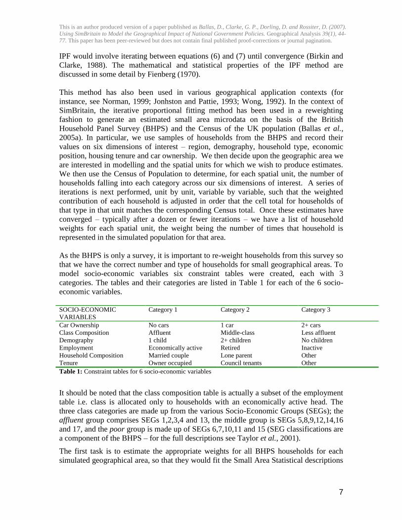
As the BHPS is only a survey, it is important to re-weight households from this survey so
that we have the correct number and type of households for small geographical areas. To
model socio-economic variables six constraint tables were created, each with 3
categories. The tables and their categories are listed in Table 1 for each of the 6 socio-
economic variables.
SOCIO-ECONOMIC
VARIABLES
Category 1 Category 2 Category 3
Car Ownership No cars 1 car 2+ cars
Class Composition Affluent Middle-class Less affluent
Demography 1 child 2+ children No children
Employment Economically active Retired Inactive
Household Composition Married couple Lone parent Other
Tenure Owner occupied Council tenants Other
Table 1: Constraint tables for 6 socio-economic variables
It should be noted that the class composition table is actually a subset of the employment
table i.e. class is allocated only to households with an economically active head. The
three class categories are made up from the various Socio-Economic Groups (SEGs); the
affluent group comprises SEGs 1,2,3,4 and 13, the middle group is SEGs 5,8,9,12,14,16
and 17, and the poor group is made up of SEGs 6,7,10,11 and 15 (SEG classifications are
a component of the BHPS – for the full descriptions see Taylor et al., 2001).
The first task is to estimate the appropriate weights for all BHPS households for each
simulated geographical area, so that they would fit the Small Area Statistical descriptions
This is an author produced version of a paper published as Ballas, D., Clarke, G. P., Dorling, D. and Rossiter, D. (2007).
Using SimBritain to Model the Geographical Impact of National Government Policies. Geographical Analysis 39(1), 44-
77. This paper has been peer-reviewed but does not contain final published proof-corrections or journal pagination.
8
described in Table 1. It should be noted that all BHPS households have already been
given a weight that compensates for error, bias, refusals etc. In particular, in wave one of
the BHPS, household weights were applied to compensate for the unequal selection
probability arising from the two-stage stratified sampling design, to compensate for non-
responding households and to adjust for those individuals in a responding household who
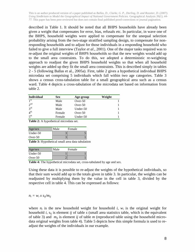
failed to give a full interview (Taylor et al., 2001). One of the major tasks required was to
re-adjust the original weights of BHPS households so that the new weights would add up
to the small area constraints. To do this, we adopted a deterministic re-weighting
approach to readjust the given BHPS household weights so that when all household
weights are added up they fit the small area constraints. This is described simply in tables
2 - 5 (following Ballas et al., 2005a). First, table 2 gives a hypothetical individual BHPS
microdata set comprising 5 individuals which fall within two age categories. Table 3
shows a census cross-tabulation table for a small geographical area such as a census
ward. Table 4 depicts a cross-tabulation of the microdata set based on information from
table 2.
Individual Sex Age-group Weight
1st Male Over-50 1
2nd
Male Over-50 1
3rd
Male Under-50 1
4th
Female Over-50 1
5th
Female Under-50 1
Table 2: A hypothetical microdata set.
Age/sex Male Female
Under-50 3 5
Over-50 3 1
Table 3: Hypothetical small area data tabulation
Age/sex Male Female
Under-50 1 1
Over-50 2 1
Table 4: The hypothetical microdata set, cross-tabulated by age and sex.
Using these data it is possible to re-adjust the weights of the hypothetical individuals, so
that their sum would add up to the totals given in table 3. In particular, the weights can be
readjusted by multiplying them by the value in the cell in table 3, divided by the
respective cell in table 4. This can be expressed as follows:
ni = wi x sij/mij
where ni is the new household weight for household i, wi is the original weight for
household i, sij is element ij of table s (small area statistics table, which is the equivalent
of table 3) and mij is element ij of table m (reproduced table using the household micro-
data original weights from table 4). Table 5 depicts how this simple formula is used to re-
adjust the weights of the individuals in our example.

This is an author produced version of a paper published as Ballas, D., Clarke, G. P., Dorling, D. and Rossiter, D. (2007).
Using SimBritain to Model the Geographical Impact of National Government Policies. Geographical Analysis 39(1), 44-
77. This paper has been peer-reviewed but does not contain final published proof-corrections or journal pagination.
9
Individual Sex age-group Org. Weight New weight
1st Male Over-50 1 1 x 3/2 = 1.5
2nd
Male Over-50 1 1 x 3/2 = 1.5
3rd
Male Under-50 1 1 x 3/1 = 3
4th
Female Over-50 1 1 x 1/1 = 1
5th
Female Under-50 1 1x 5/1 = 5
Table 5: Reweighting the hypothetical microdata set in order to fit table 3.
One of the difficulties encountered with the reweighting methodology described above
was the high presence of BHPS households coming from geographical areas other than
the simulated area (in particular, there was a high presence of households from the South
East of England in the simulation of other regions). Table 6 shows the geographical
distribution of the households in the BHPS wave 1. As can be seen, around 33% of the
households come from the South East, whereas only about 10% of households come from
Yorkshire and the Humber.
Value Label Frequency Frequency (%)
Inner London 1 498 5.8
Outer London 2 597 7
Rest of South East 3 1611 18.9
South West 4 713 8.4
East Anglia 5 303 3.6
East Midlands 6 595 7
West Midlands Conurb 7 391 4.6
Rest of West Midlands 8 369 4.3
Greater Manchester 9 396 4.6
Merseyside 10 195 2.3
Rest of North West 11 363 4.3
South Yorkshire 12 197 2.3
West Yorkshire 13 299 3.5
Rest of Yorks & Humber 14 257 3
Tyne & Wear 15 202 2.4
Rest of North 16 293 3.4
Wales 17 392 4.6
Scotland 18 853 10
Table 6: Origin of wave 1 BHPS households (AREGION)
In the case of the simulation of the population in York the initial geographical
distribution of the BHPS households would result in the selection of large numbers of
non-Northern households from wave 1 that would populate the York wards. In order to
deal with this problem we explored a number of possible solutions and concluded that the
best approach was to define the BHPS sample used in the simulation on the basis of the
geographical area being simulated. For instance, in the simulation of York we used only
the BHPS households that lived in the BHPS region Rest of Yorkshire and Humber
(AREGION = 14).

This is an author produced version of a paper published as Ballas, D., Clarke, G. P., Dorling, D. and Rossiter, D. (2007).
Using SimBritain to Model the Geographical Impact of National Government Policies. Geographical Analysis 39(1), 44-
77. This paper has been peer-reviewed but does not contain final published proof-corrections or journal pagination.
10
After generating the BHPS household weights for each ward in York, the next step was to
select the appropriate households (or, in other words, convert the decimal weights or
probabilities into integer weights). Thus, we developed and tested different “integer
weighting” or integerisation methodologies and we concluded that the following
methodology represented the best solution:
Define two variables named counter and weight and set them to zero and then:
Sort all households into ascending order of probability of living in the small area
(which were calculated using the method described above) being populated
Increase cumulative weight by the weight (probability) of the next sorted household
h(counter). For instance, if counter = 0, the weight is increased by the probability of
the first household: h(0)
If cumulative weight > 1 give to the household h(counter) an integer weight equal to
the rounded weight value and subtract this value from weight (e.g. if weight = 2.05
set household weight = 2 and set weight = 2.05 –2 = 0.05). Increase counter by 1
(move to next household)
If counter < total number of households in the small area, return to step 2, else exit.
The implementation of the above algorithm led to the creation of a ward-level micro-data
set for the city of York. However, we observed that there were, in some wards, relatively
high over-estimates and under-estimates of some variables especially those that were not
used as constraints in the simulation. In order to tackle this problem we developed an
algorithm aimed at swapping suitable simulated households between wards in order to
further reduce the error. The steps taken to reduce the error were as follows:
Identify wards with the highest over-estimate and under-estimates for each
variable
Compare each household in the simulated database with all other household and
search for households that have all attributes in common but one.
For each pair of almost identical households swap the households between the
areas with the highest over-estimate and under-estimate.
Move to the next household and repeat the process.
A more detailed discussion of the SimBritain static modelling process appears in Ballas
et al. (2005a).
4 Projecting small area statistics into the future
4.1 Population updating
This section provides more details on the procedures for estimating key variables within
the dynamic microsimulation model SimBritain. The demographic variables can be
updated by simulating the processes of mortality, fertility and internal migration. Other

This is an author produced version of a paper published as Ballas, D., Clarke, G. P., Dorling, D. and Rossiter, D. (2007).
Using SimBritain to Model the Geographical Impact of National Government Policies. Geographical Analysis 39(1), 44-
77. This paper has been peer-reviewed but does not contain final published proof-corrections or journal pagination.
11
socio-economic variables have to be updated using some form of trend analysis (see
section 4.2). These can then form the base scenarios for future predictions. A number of
what-ifs can be tested to analyse the stability of these forecasts (pertubations from
existing trends caused by policy etc).
In the models mortality and fertility are based on location specific probabilities. Fertility
is also assumed to be a function of age, marital status and location. Births can be
modelled using five-year age groups and marital status data available for each
ward/county from the Census. Every synthetic female in the database is tested for
eligibility to give birth. Monte Carlo sampling against the fertility probabilities is used to
determine which females give birth. If a birth is deemed to occur, the model creates a
new individual. The new individual‟s attributes are set as follows: age is zero, sex is
determined probabilistically (a slightly higher probability of male than female sex),
marital status is single, social class and location are that of the mother and all other
attributes are left blank. In the next simulation period, the new individual is simulated
along with the other individuals in the location.
It can be argued that spatial microsimulation provides the ideal basis for the modelling of
spatial transitions such as migration. In particular, the propensity to migrate is heavily
dependent on household and individual attributes and therefore a micro-level approach
may be the most appropriate to estimate and model migration for different types of
individuals. For instance, Rogerson and Plane (1998) emphasise the role of age and
tenure in household mobility and migration decision making:
It is well known that mobility rates are substantially higher among renters than among
homeowners. Similarly, the age structure of migrants to and from neighborhoods is
likely to be quite different in a neighborhood comprised primarily of homeowners in
comparison with a renter-dominated neighborhood.
(Rogerson and Plane, 1998: 1468)
The current version of SimBritain does not model migration explicitly, although the
population trend analysis discussed in the following section is implicitly affected by
migration trends, which are captured in the overall population change. Nevertheless, we
are currently investigating ways of enhancing the migration modelling capabilities of
SimBritain, by adopting methods such as those discussed by Ballas et al., 2005b).
4.2. Socio-economic variables
Traditionally in the social sciences, it has been far more difficult to update or forecast
other socio-economic variables, which may largely depend on a variety of external
factors (factory closures, new housing development etc). In order to project the socio-
economic characteristics of the population of Britain into 2001, 2011 and 2021 we used
data from previous Censuses to project forward (on an all else being equal extrapolation
basis) the changing patterns or trends for every socio-economic variables under
consideration. In particular, projections of small area statistics tables were calculated
using the 1971, 1981 and 1991 Census Small Area Statistics (SAS). Using these three
This is an author produced version of a paper published as Ballas, D., Clarke, G. P., Dorling, D. and Rossiter, D. (2007).
Using SimBritain to Model the Geographical Impact of National Government Policies. Geographical Analysis 39(1), 44-
77. This paper has been peer-reviewed but does not contain final published proof-corrections or journal pagination.
12
time points, a trend curve was produced allowing tables to be predicted up to 2021. The
projections of future small area statistics tables were undertaken at ward level.
Projections for 2001:
32 ))/(lnln)(lnexp(ln vuwWA (9)
Projections for 2011:
32 ))/(lnln)(lnexp(ln wvxAB (10)
Projections for 2021:
32 ))/(lnln)(lnexp(ln xwyBC (11)
where
u = smoothed proportion in 1971
v = smoothed proportion in 1981
w = smoothed proportion in 1991
x = smoothed proportion in 2001
y = smoothed proportion in 2011
z = smoothed proportion in 2021
W = ward proportion in 1991
A = ward proportion in 2001
B = ward proportion in 2011
C = ward proportion in 2021
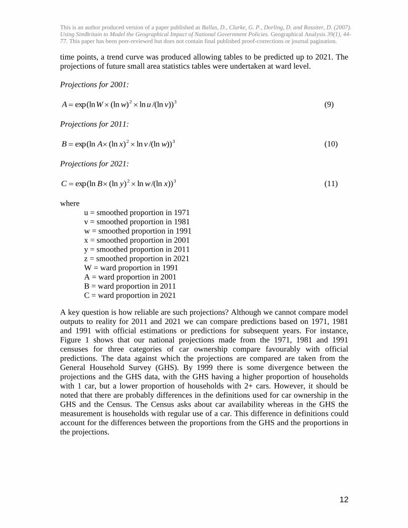
A key question is how reliable are such projections? Although we cannot compare model
outputs to reality for 2011 and 2021 we can compare predictions based on 1971, 1981
and 1991 with official estimations or predictions for subsequent years. For instance,
Figure 1 shows that our national projections made from the 1971, 1981 and 1991
censuses for three categories of car ownership compare favourably with official
predictions. The data against which the projections are compared are taken from the
General Household Survey (GHS). By 1999 there is some divergence between the
projections and the GHS data, with the GHS having a higher proportion of households
with 1 car, but a lower proportion of households with 2+ cars. However, it should be
noted that there are probably differences in the definitions used for car ownership in the
GHS and the Census. The Census asks about car availability whereas in the GHS the
measurement is households with regular use of a car. This difference in definitions could
account for the differences between the proportions from the GHS and the proportions in
the projections.
This is an author produced version of a paper published as Ballas, D., Clarke, G. P., Dorling, D. and Rossiter, D. (2007).
Using SimBritain to Model the Geographical Impact of National Government Policies. Geographical Analysis 39(1), 44-
77. This paper has been peer-reviewed but does not contain final published proof-corrections or journal pagination.
13
0
0.1
0.2
0.3
0.4
0.5
0.6
1971 1976 1981 1986 1991 1996 2001 2006 2011 2016 2021
Year
Pro
po
rtio
n
no car 1 car 2+ cars
GHS - no car GHS - 1 car GHS - 2+ cars
Figure 1: Car ownership in Great Britain, 1971-2021
Similar comparisons of the simulated trends in other variables (e.g. household types,
tenure, etc) were carried out and showed equally good model fits on the short-term future.
For more „calibration‟ of results see Ballas et al. (2005a).
Another way of checking the reliability of our projection methodology is by using past
Census data to project distributions of populations into 1991 and then compare the
projected values with the actual data from the 1991 Census (and 2001 now that the full
UK census results are published). Table 7 shows an example of a comparison of Census
data on social class groupings and projected proportions of these groups in 1991. As can
be seen, by using the data on social class for the years 1961-71-81 our projection method
predicts that 34% of the households in York in 1991 would belong to Class I and II. This
prediction matches the actual proportion (to the nearest percentile), which was calculated
with the use of 1991 Census data. Likewise, our projection method works very well in
estimating the 1991 distributions of Class III, IV & V households (but least well for the
last two groups where more people remained in these classes than projections would
suggest).
Census data
Year 1951 1961 1971 1981 1991 Predicted
proportion for
1991
Difference between
projection and
actual data
Class I & II 19% 21% 24% 28% 34% 34% 0%
Class III 51% 50% 49% 47% 43% 44% 1%
ClassIV & V 30% 29% 27% 25% 24% 22% -2%
Table 7: Comparing Census data to projected data for 1991 (projection based on data from the Censuses of
1961, 1971 and 1981)
It would be reasonable to expect that the performance of the model would vary from
variable to variable, especially at areas as small as wards and for variables, which were
not included as constraints in the simulation exercise; but it is also interesting to see
This is an author produced version of a paper published as Ballas, D., Clarke, G. P., Dorling, D. and Rossiter, D. (2007).
Using SimBritain to Model the Geographical Impact of National Government Policies. Geographical Analysis 39(1), 44-
77. This paper has been peer-reviewed but does not contain final published proof-corrections or journal pagination.
14
which kinds of socio-economic variable are hardest to predict across space. It should be
noted that the model is more reliable when analysing socio-economic patterns at the level
of the city rather than ward. At the ward level the performance of the model varies
considerably and there is a need to introduce further constraints in order to perform
analysis at the ward or sub-ward level for particular variables. This is on-going research,
but – and in hindsight most obviously – where a university is located in a particular city
tends to alter the social trajectories of wards near that university as student numbers rise
rapidly. Many other examples can be easily envisaged connected with the decline of
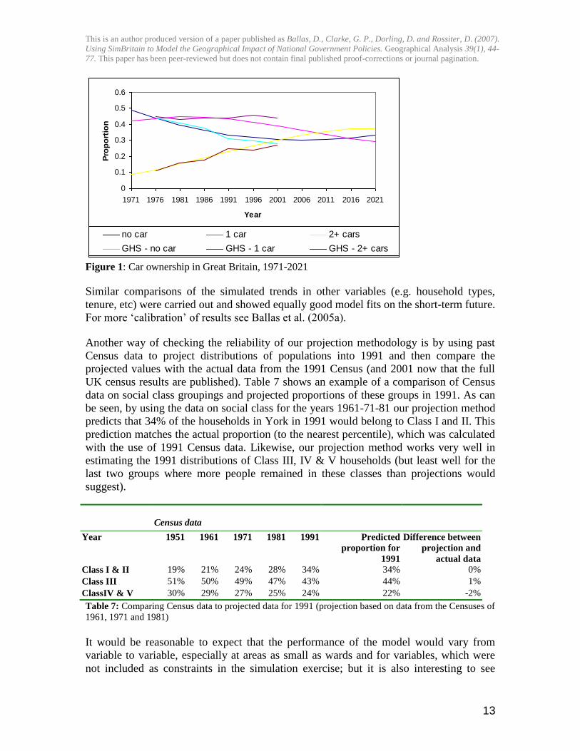
traditional manufacturing, changes in transport infrastructure and so on. Figures 2 and 3
show the scatterplot for two of the projected variables at the ward and parliamentary
constituency level, the Census proportion on the vertical and the simulated proportion on
the horizontal axis. A perfect match would find all points on a straight line of gradient 1.
As can be seen in Figure 2, there is a relatively good match of simulated and actual
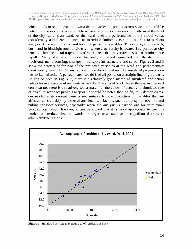
values for average age of residents across the 15 wards of York. Nevertheless, as Figure 3
demonstrates there is a relatively worst match for the values of actual and simulated rate
of travel to work by public transport. It should be noted that, as figure 3 demonstrates,
our model in its current form is not suitable for the prediction of variables that are
affected considerably by external and localised factors, such as transport networks and
public transport services, especially when the analysis is carried out for very small
geographical units. However, it can be argued that it is more appropriate to use this
model to simulate electoral wards or larger areas such as metropolitan districts or
administrative regions.
Average age of residents by ward, York 1991
30.0
32.0
34.0
36.0
38.0
40.0
42.0
44.0
46.0
48.0
50.0
30.0 35.0 40.0 45.0 50.0
Simulated
Ce
ns
us
Ward data
York
Figure 2: Simulated vs. actual average age of residents in York
This is an author produced version of a paper published as Ballas, D., Clarke, G. P., Dorling, D. and Rossiter, D. (2007).
Using SimBritain to Model the Geographical Impact of National Government Policies. Geographical Analysis 39(1), 44-
77. This paper has been peer-reviewed but does not contain final published proof-corrections or journal pagination.
15
Travel to work by public transport, York 1991
0.0%
2.0%
4.0%
6.0%
8.0%
10.0%
12.0%
14.0%
0.0% 2.0% 4.0% 6.0% 8.0% 10.0% 12.0% 14.0%
Simulated (%)
Ce
ns
us (
%)
Ward data
York
Figure 3: Simulated vs. actual rate of working population travelling to work by public transport in York
It should be noted that it is likely that variables highly correlated with any of the
constraints will be relatively well predicted. In addition, as sampling error in the BHPS
results in any of the constraint variables deviating from the national average as given in
the Census, this should be rectified by the need to ensure that the constraints are, as far as
possible, met. Insofar as sampling error in the BHPS results in any of the test variables
deviating from the national average as measured by the Census, this will not only be
rectified indirectly, if at all. Ideally the test variable predictions and the actual Census
values will fall along a straight line with intercept=0 slope=1 – „the line of identity‟. The
This is an author produced version of a paper published as Ballas, D., Clarke, G. P., Dorling, D. and Rossiter, D. (2007).
Using SimBritain to Model the Geographical Impact of National Government Policies. Geographical Analysis 39(1), 44-
77. This paper has been peer-reviewed but does not contain final published proof-corrections or journal pagination.
16
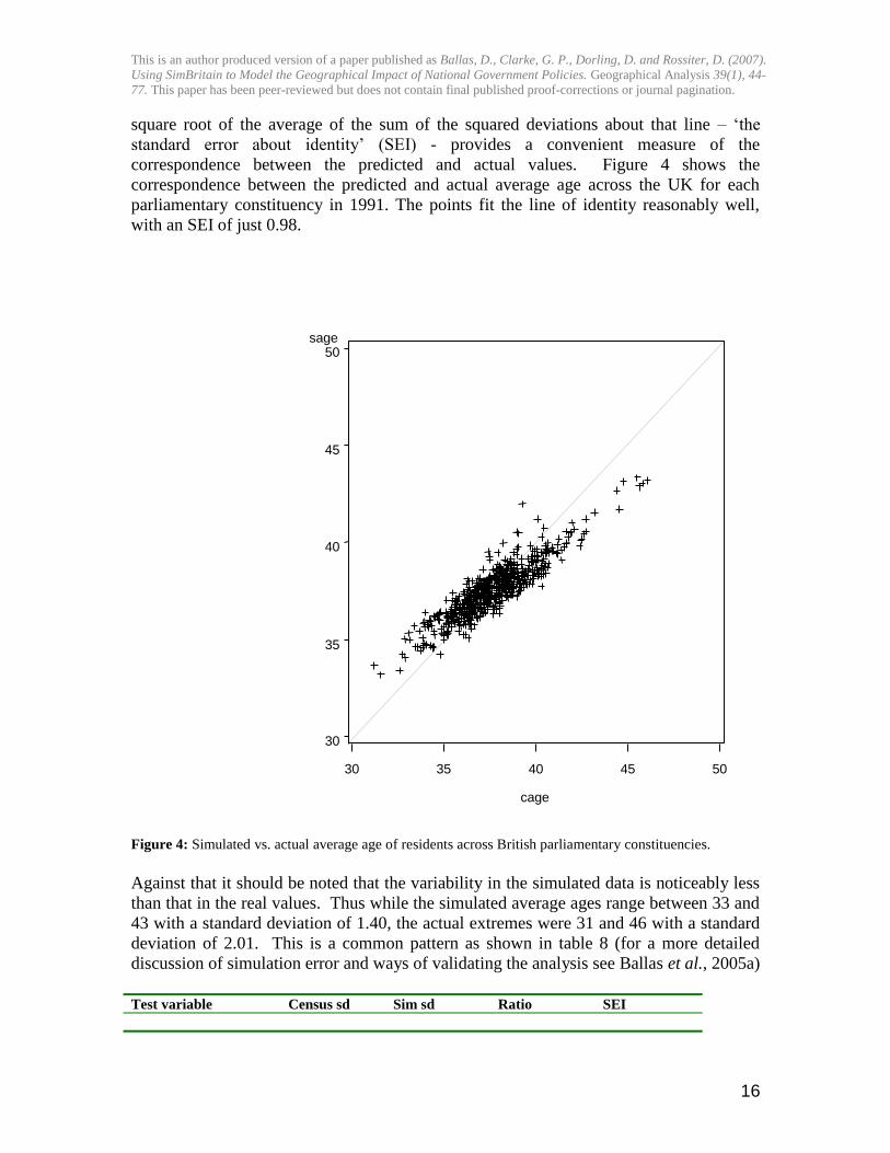
square root of the average of the sum of the squared deviations about that line – „the
standard error about identity‟ (SEI) - provides a convenient measure of the
correspondence between the predicted and actual values. Figure 4 shows the
correspondence between the predicted and actual average age across the UK for each
parliamentary constituency in 1991. The points fit the line of identity reasonably well,
with an SEI of just 0.98.
sage
30
35
40
45
50
cage
30 35 40 45 50
Figure 4: Simulated vs. actual average age of residents across British parliamentary constituencies.
Against that it should be noted that the variability in the simulated data is noticeably less
than that in the real values. Thus while the simulated average ages range between 33 and
43 with a standard deviation of 1.40, the actual extremes were 31 and 46 with a standard
deviation of 2.01. This is a common pattern as shown in table 8 (for a more detailed
discussion of simulation error and ways of validating the analysis see Ballas et al., 2005a)
Test variable Census sd Sim sd Ratio SEI
This is an author produced version of a paper published as Ballas, D., Clarke, G. P., Dorling, D. and Rossiter, D. (2007).
Using SimBritain to Model the Geographical Impact of National Government Policies. Geographical Analysis 39(1), 44-
77. This paper has been peer-reviewed but does not contain final published proof-corrections or journal pagination.
17
Male .008 .013 1.6 .011
Migrant .020 .015 0.7 .014
Age 2.01 1.40 0.7 0.98
Unemployment .041 .029 0.7 .023
Long-term ill .034 .019 0.6 .022
Detached .138 .049 0.4 .104
No heating .095 .027 0.3 .085
Public transport .142 .028 0.2 .124
Ethnicity .065 .006 0.1 .062
Table 8: Actual and simulated data for a selection of variables
5. SimBritain outputs
5.1 Predictions based on trend analysis
In this section we present some preliminary results of the SimBritain project. As noted
above, the SimBritain model was based on a pilot study of the city of York. This section
discusses some of the results of the York simulation. First, we look at how the key
variables may look for York over the next two decades given the assumption that existing
trends continue. Then, in section 4.2, we look at how changes in key social policies are
likely to influence the pattern of change.
In order to explore the likely changing social geography of York for both sets of
scenarios, we classified the simulated households into the following 5 groups:
Very poor, comprising all households with equivalised income below or equal to the
half of the median income of York.
Poor, comprising all households with equivalised income greater than half of the
median and smaller than or equal to three quarters of the median
Below-average class, comprising all households with equivalised income greater than
three quarters of the median and smaller than or equal to the median
Above-average, comprising all households with equivalised income greater than the
median and smaller than or equal to the median plus a quarter of the median
Affluent, comprising all households with equivalised income greater than the median
plus a quarter of the median
Table 9 shows the absolute and relative sizes of each household class throughout the
simulation period for the city of York.
Class size by year Very poor Poor Below average Above average Affluent Total number of
households
1991 7190 7149 6589 5322 15605 41855
2001 8208 9373 6020 6753 16848 47202
2011 9085 9149 7303 8293 17244 51074
2021 11700 6222 9476 11185 16213 54796
Class size (% of all households) by year
1991 17.2% 17.1% 15.7% 12.7% 37.3% 100.0%

This is an author produced version of a paper published as Ballas, D., Clarke, G. P., Dorling, D. and Rossiter, D. (2007).
Using SimBritain to Model the Geographical Impact of National Government Policies. Geographical Analysis 39(1), 44-
77. This paper has been peer-reviewed but does not contain final published proof-corrections or journal pagination.
18
2001 17.3% 19.9% 12.8% 14.3% 35.7% 100.0%
2011 17.8% 17.9% 14.3% 16.2% 33.8% 100.0%
2021 21.3% 11.4% 17.3% 20.4% 29.6% 100.0%
Table 9: The size of the simulated household classes, 1991-2021
It should be noted that the above classification encapsulates an implicit definition of
poverty, by describing the lower income households as poor and very poor. This is a
definition of relative poverty, as it is not directly based on the degree to which
households are able to satisfy their physiological or other basic needs. However, given
that the analysis presented here projects the population of York into the future, it can be
argued that income should be used to define and analyse poverty, as it will be likely to
keep its significance through time, whereas human needs and social roles will evolve.
In the remainder of this section we explore the living standards of the simulated
households throughout the 30-year simulation period. In one of the first detailed studies
of poverty, Rowntree (2000) described the quality of life of his different household
classes in York and then set out to explore the incidence of some variables described as
immediate causes of poverty. One of the aims of our model has been to simulate a survey
similar to Rowntree‟s original study of York.
It is interesting to note that according to the simulation the the poorest segment of the
York society (very poor households, as described above) is predicted as a group to
increase in size, from 17.2% of total households in 1991 to 21.3% in 2021. Further, the
number of children living in very poor households rises significantly from 21.8% in 1991
(as a percentage of all children in York) to 38.5% in 2021. Likewise, the number of
elderly people in this group increases from 30.1% in 1991 to 44.2% in 2021. The
incidence of Limiting Long Term Illness (LLTI) is estimated to be 9% in 1991 and is
predicted to fall to 7.9% by 2021. Further, an estimated 10.6% of the population in 1991
report anxiety and depression problems. Table 10 sheds more light on the prospects for
households in the very poor category.
Very poor households 1991 2001 2011 2021
Households (% of all households in York) 17.2% 17.3% 17.8% 21.3%
Individuals (% of all individuals in York) 14.7% 13.3% 13.7% 20.5%
Children (% of all children in York) 21.8% 17.7% 18.6% 38.5%
LLTI (as a % of all individuals in group) 9.0% 7.3% 5.4% 7.9%
Elderly (over 64 years as a % of all individuals in group) 30.1% 32.0% 33.3% 44.2%
Individuals in group with father's occupation: unskilled (%) 10.5% 6.8% 3.3% 15.1%
Reporting anxiety and depression (% of all individuals in group) 10.6% 10.3% 7.4% 3.1%
Individuals who reported that they have no one to talk to 19.9% 23.8% 31.1% 31.5%
Promotion opportunities in current job (as % of individuals with
a job) 33.7% 36.9% 51.9% 79.7%
Feeling unhappy or depressed 19.9% 19.0% 18.2% 12.1%
Home computer in accommodation 1.4% 1.0% 0.5% 0.4%
House without central heating 26.1% 21.4% 21.4% 31.1%
Single-person households 61.6% 76.0% 77.9% 64.4%
Cars/Households ratio 0.23 0.32 0.38 0.40
Table 10: Living standards of very poor households
This is an author produced version of a paper published as Ballas, D., Clarke, G. P., Dorling, D. and Rossiter, D. (2007).
Using SimBritain to Model the Geographical Impact of National Government Policies. Geographical Analysis 39(1), 44-
77. This paper has been peer-reviewed but does not contain final published proof-corrections or journal pagination.
19
It is interesting to note that in 1991 we estimated that 10.5% of very poor households
have a household head whose father had an unskilled occupation. This percentage is
projected to rise in 2021 to 15.1%. A useful indicator of well-being and prosperity is the
ratio of cars/households, especially given that there is a general increasing trend in car
ownership across all households in the simulation period. Nevertheless, there are only
slight increases in this ratio in the very poor households, in the period 1991-2011. The
ratio increases from 0.23 in 1991 to 0.40 in 2021. In affluent households this variable
increases from 0.94 to 1.72. Further, the percentage of households that have a home
computer is estimated to be 1.4% in 1991 and it is projected to drop to 0.4% in 2021. It
should be noted though that this projection is not very realistic, given that home
computers become increasingly common in households. However, the home computer
here may be seen as the equivalent of a high tech product at any time (e.g. in 2001 it
could be a DVD player or mobile phone with photo-messaging and in 2021 it may be
virtual reality facilities or some other product or service).
Moreover, it is worth noting that only 33.7% of individuals who have a job felt that they
have opportunities for promotion in 1991. This percentage increases to 79.7% by 2021.
Also, 31.1% feel that they struggle financially in 1991. Yet this proportion also has a
falling trend and is projected to be only 16.2% in 2021.
Very poor households 1991 2001 2011 2021
Unemployed (as a % of economically active in group) 45.4% 25.7% 16.7% 9.6%
Economically active (%) 18.3% 17.1% 16.8% 17.7%
Vocational qualifications (% of all adult individuals in group) 20.9% 20.7% 18.9% 12.2%
Full-time job (% of economically active in group) 43.1% 65.9% 80.7% 90.1%
Adults with no qualifications (%of all adult individuals in group) 58.4% 65.2% 72.3% 78.9%
Table 11: Very poor households, possible causes of poverty
As it can be seen, almost half (45.4%) of the economically active individuals living in
very poor households are unemployed in 1991. It therefore seems that although
unemployment remains an important determinant of poverty there are other factors that
contribute significantly to poverty (see table 11), as the simulation predicts near-full
employment conditions in the future. It is also interesting to note that this was one of the
conclusions in Rowntree‟s work:
An analysis of persons in the city who are below the “primary” poverty line shows that more than
one half of these are members of families whose wage-earner is in work but in receipt of insufficient
wages.
Rowntree (2000: 114)
Table 11 shows that there is an increasing trend in the proportion of individuals without
any qualifications living in very poor households. Also, there is a decreasing trend in the
numbers of individuals with vocational qualifications. It can be argued that the lack of
educational qualifications may be one of the major causes of low pay and limited chances
of finding a secure well-paid job. It should be noted though that given the increasing
trend in general education levels, the no qualifications variable in the future may mean
This is an author produced version of a paper published as Ballas, D., Clarke, G. P., Dorling, D. and Rossiter, D. (2007).
Using SimBritain to Model the Geographical Impact of National Government Policies. Geographical Analysis 39(1), 44-
77. This paper has been peer-reviewed but does not contain final published proof-corrections or journal pagination.
20
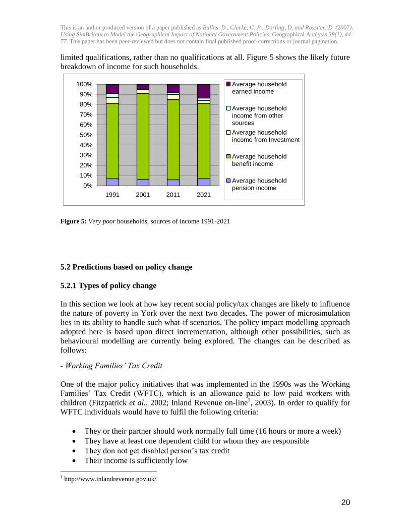
limited qualifications, rather than no qualifications at all. Figure 5 shows the likely future
breakdown of income for such households.
0%
10%
20%
30%
40%
50%
60%
70%
80%
90%
100%
1991 2001 2011 2021
Average householdearned income
Average householdincome from othersources
Average householdincome from Investment
Average householdbenefit income
Average householdpension income
Figure 5: Very poor households, sources of income 1991-2021
5.2 Predictions based on policy change
5.2.1 Types of policy change
In this section we look at how key recent social policy/tax changes are likely to influence
the nature of poverty in York over the next two decades. The power of microsimulation
lies in its ability to handle such what-if scenarios. The policy impact modelling approach
adopted here is based upon direct incrementation, although other possibilities, such as
behavioural modelling are currently being explored. The changes can be described as
follows: - Working Families’ Tax Credit
One of the major policy initiatives that was implemented in the 1990s was the Working
Families‟ Tax Credit (WFTC), which is an allowance paid to low paid workers with
children (Fitzpatrick et al., 2002; Inland Revenue on-line1, 2003). In order to qualify for
WFTC individuals would have to fulfil the following criteria:
They or their partner should work normally full time (16 hours or more a week)
They have at least one dependent child for whom they are responsible
They don not get disabled person‟s tax credit
Their income is sufficiently low
1 http://www.inlandrevenue.gov.uk/
This is an author produced version of a paper published as Ballas, D., Clarke, G. P., Dorling, D. and Rossiter, D. (2007).
Using SimBritain to Model the Geographical Impact of National Government Policies. Geographical Analysis 39(1), 44-
77. This paper has been peer-reviewed but does not contain final published proof-corrections or journal pagination.
21
Their savings and capital are not worth more than £8,000
They are present and ordinarily resident in Great Britain
They are not subject to immigration control
WFTC is calculated by comparing the family income with the applicable amount or
threshold figure, which in 2002 was £94.50. If the family income is less than the
applicable amount, then the family receives the maximum WTFC. If the family income
exceeds the applicable amount, the maximum WFTC is reduced by 55% of the excess
(Fitzpatrick et al., 2002). As noted above, in the context of the research reported here all
the relative amounts were adjusted to allow for inflation. In the case of WFTC the
applicable amount of £94.50 in 2002 was readjusted to its equivalent in 1991 on the basis
of the RPI growth of 29.3%. Thus, the adjusted applicable amount that we used was
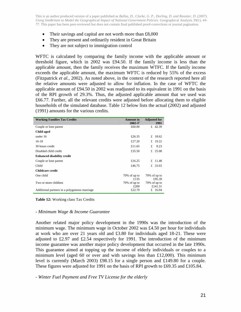
£66.77. Further, all the relevant credits were adjusted before allocating them to eligible
households of the simulated database. Table 12 below lists the actual (2002) and adjusted
(1991) amounts for the various credits.
Working Families Tax Credits Amount in
2002-31
Adjusted for
1991
Couple or lone parent £60.00 £ 42.39
Child aged
under 16 £26.35 £ 18.62
16-18 £27.20 £ 19.22
30 hours credit £11.65 £ 8.23
Disabled child credit £35.50 £ 25.08
Enhanced disability credit
Couple or lone parent £16.25 £ 11.48
Child £46.75 £ 33.03
Childcare credit
One child 70% of up to £135
70% of up to £95.39
Two or more children 70% of up to
£200
70% of up to
£141.31 Additional partners in a polygamous marriage £22.70 £ 16.04
Table 12: Working class Tax Credits
- Minimum Wage & Income Guarantee
Another related major policy development in the 1990s was the introduction of the
minimum wage. The minimum wage in October 2002 was £4.50 per hour for individuals
at work who are over 21 years old and £3.80 for individuals aged 18-21. These were
adjusted to £2.97 and £2.54 respectively for 1991. The introduction of the minimum
income guarantee was another major policy development that occurred in the late 1990s.
This guarantee aimed at topping up the income of elderly individuals or couples to a
minimum level (aged 60 or over and with savings less than £12,000). This minimum
level is currently (March 2003) £98.15 for a single person and £149.80 for a couple.
These figures were adjusted for 1991 on the basis of RPI growth to £69.35 and £105.84.
- Winter Fuel Payment and Free TV License for the elderly

This is an author produced version of a paper published as Ballas, D., Clarke, G. P., Dorling, D. and Rossiter, D. (2007).
Using SimBritain to Model the Geographical Impact of National Government Policies. Geographical Analysis 39(1), 44-
77. This paper has been peer-reviewed but does not contain final published proof-corrections or journal pagination.
22
Another policy initiative which aimed at boosting the incomes of the elderly was the
Winter Fuel Payment, which is given to individuals aged 60 or over. This amount was
£200 in 2003 and was adjusted to £141.31 for 1991. Further, a similar government
initiative was the provision of free or reduced TV licenses to all individuals aged 75 or
over. In the case of TV license there is no need to readjust the 2002-3 figure to 1991 as
data exist on the TV license across time. The TV license was £112 in 2002, whereas in
1991 it was £771.
5.2.2 Impacts of Policy Changes
Once all the figures were adjusted the next step was to estimate the redistributive effects
that these policies would have if they had been implemented in each of the simulation
years. It is interesting to note that the suggested policies would have a great impact on
families with children. For instance, according to the 1991 simulation outputs, there
would be 246 children living in families whose income would increase by 54.1% (these
are the poorest households of the very poor class). Further, there would be 486 children
living in families, which would experience income increases of over 15.4%. It is
interesting to use the BHPS to draw a picture of typical households, which would be
affected by the policy changes. Below there is a description of typical simulated
households that would be most affected by the 1990s welfare reforms:
Age of
household
head(s)
Description
18 and 18 Married couple, 1 newborn baby. Male no qualifications, working in sales
and services female General Certificate of Education (GCE)O LEVELS, in
family care (formerly employed in sales and services). Weekly expenditure
on food: £20. Household income before policy effects: £6,265.34. Income
after policy effects: £9,656.62 (increase of 54.1%). No car
26 and 22 Married couple, 1 child aged 3. £9,230.02; both in full employment, full
time. Male plant and machine operative, female sales and services. Male
has Certificate of Secondary Education (CSE) (Grade 2-5) qualifications.
Female has GCE O Levels. Average food expenditure per week: £30. 1
car. Income after policy change: £11,952.44 (increase 29.5%)
It is also interesting to note that the model suggests that several households would change
class (e.g. from very poor to poor) under the suggested changes. Table 13 lists the class
transitions by year.
Class Transitions in 1991 Households % of all households
From very poor to poor 3720 8.89%
From poor to below average 1137 2.72%
From below average to over average 774 1.85%
From above average to affluent 866 2.07%
Class Transitions in 2001
From very poor to poor 2782 5.89%
From poor to below average 770 1.63%
From below average to over average 790 1.67%
This is an author produced version of a paper published as Ballas, D., Clarke, G. P., Dorling, D. and Rossiter, D. (2007).
Using SimBritain to Model the Geographical Impact of National Government Policies. Geographical Analysis 39(1), 44-
77. This paper has been peer-reviewed but does not contain final published proof-corrections or journal pagination.
23
From above average to affluent 824 1.75%
Class Transitions in 2011
From very poor to poor 1150 2.25%
From poor to below average 617 1.21%
From below average to over average 2565 5.02%
From above average to affluent 1652 3.23%
Class Transitions in 2021
From very poor to poor 2280 4.16%
From poor to below average 3238 5.91%
From below average to over average 54 0.10%
From above average to affluent 259 0.47%
Table 13: Class transitions triggered by policy changes
As can be seen the larger number of class transitions would occur had the policies been
adopted in 1991, when 3720 households would have moved from the very poor to poor.
Another way of examining the impact of the above policy change is by analysing the
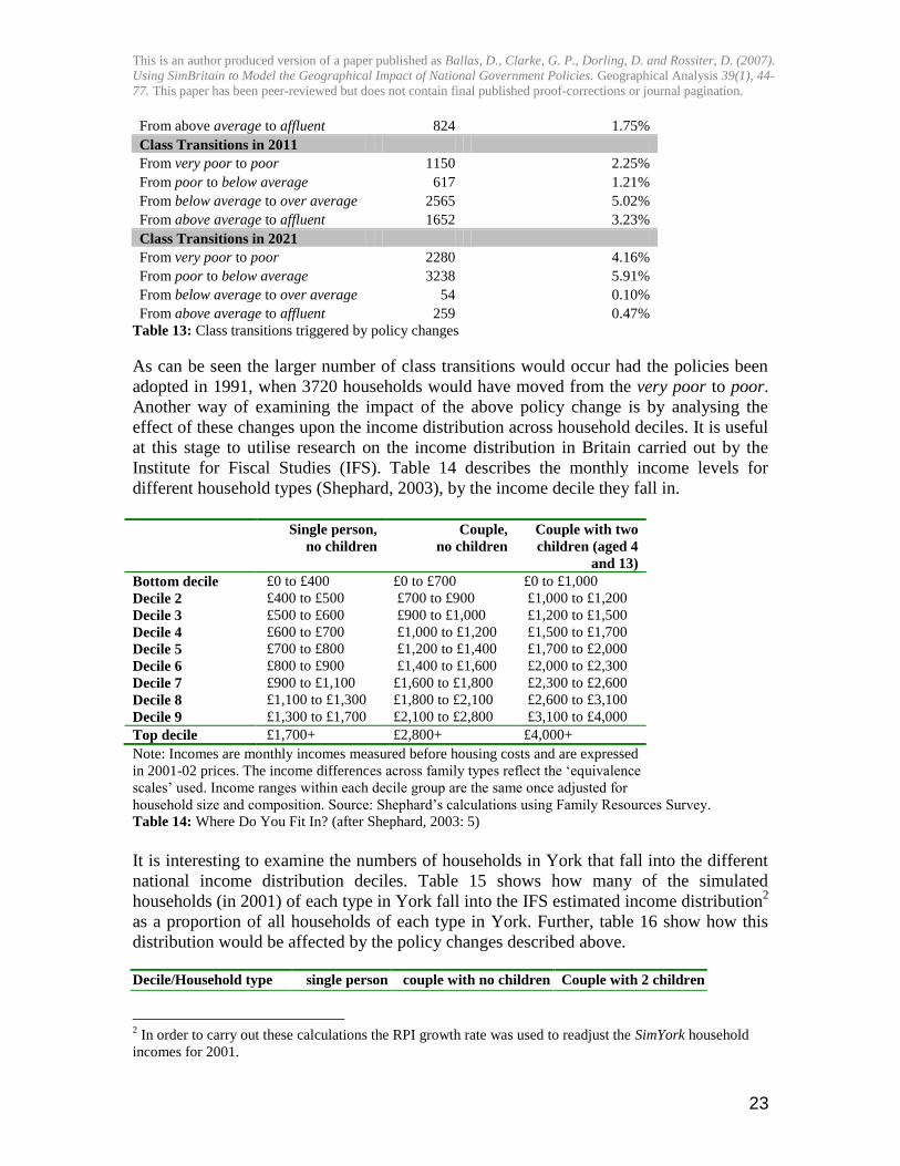
effect of these changes upon the income distribution across household deciles. It is useful
at this stage to utilise research on the income distribution in Britain carried out by the
Institute for Fiscal Studies (IFS). Table 14 describes the monthly income levels for
different household types (Shephard, 2003), by the income decile they fall in.
Single person,
no children
Couple,
no children
Couple with two
children (aged 4
and 13)
Bottom decile £0 to £400 £0 to £700 £0 to £1,000
Decile 2 £400 to £500 £700 to £900 £1,000 to £1,200
Decile 3 £500 to £600 £900 to £1,000 £1,200 to £1,500
Decile 4 £600 to £700 £1,000 to £1,200 £1,500 to £1,700
Decile 5 £700 to £800 £1,200 to £1,400 £1,700 to £2,000
Decile 6 £800 to £900 £1,400 to £1,600 £2,000 to £2,300
Decile 7 £900 to £1,100 £1,600 to £1,800 £2,300 to £2,600
Decile 8 £1,100 to £1,300 £1,800 to £2,100 £2,600 to £3,100
Decile 9 £1,300 to £1,700 £2,100 to £2,800 £3,100 to £4,000
Top decile £1,700+ £2,800+ £4,000+
Note: Incomes are monthly incomes measured before housing costs and are expressed
in 2001-02 prices. The income differences across family types reflect the „equivalence
scales‟ used. Income ranges within each decile group are the same once adjusted for
household size and composition. Source: Shephard‟s calculations using Family Resources Survey. Table 14: Where Do You Fit In? (after Shephard, 2003: 5)
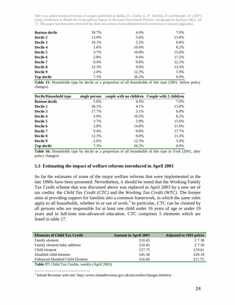
It is interesting to examine the numbers of households in York that fall into the different
national income distribution deciles. Table 15 shows how many of the simulated
households (in 2001) of each type in York fall into the IFS estimated income distribution2
as a proportion of all households of each type in York. Further, table 16 show how this
distribution would be affected by the policy changes described above.
Decile/Household type single person couple with no children Couple with 2 children
2 In order to carry out these calculations the RPI growth rate was used to readjust the SimYork household
incomes for 2001.
This is an author produced version of a paper published as Ballas, D., Clarke, G. P., Dorling, D. and Rossiter, D. (2007).
Using SimBritain to Model the Geographical Impact of National Government Policies. Geographical Analysis 39(1), 44-
77. This paper has been peer-reviewed but does not contain final published proof-corrections or journal pagination.
24
Bottom decile 30.7% 4.4% 7.0%
Decile 2 13.9% 5.6% 13.8%
Decile 3 16.1% 2.2% 6.8%
Decile 4 1.6% 10.4% 8.2%
Decile 5 3.7% 10.8% 15.6%
Decile 6 2.8% 9.4% 17.2%
Decile 7 9.4% 9.8% 12.1%
Decile 8 12.3% 9.0% 13.3%
Decile 9 2.0% 12.3% 5.9%
Top decile 7.3% 26.2% 0.0%
Table 15: Households type by decile as a proportion of all households of this type (2001, before policy
changes)
Decile/Household type single person couple with no children Couple with 2 children
Bottom decile 5.6% 4.4% 7.0%
Decile 2 36.1% 4.1% 13.8%
Decile 3 17.7% 3.1% 6.8%
Decile 4 3.0% 10.5% 8.2%
Decile 5 3.7% 5.9% 15.6%
Decile 6 2.8% 14.8% 11.6%
Decile 7 9.4% 9.8% 17.7%
Decile 8 12.3% 9.0% 13.3%
Decile 9 2.0% 12.3% 5.9%
Top decile 7.3% 26.2% 0.0%
Table 16: Households type by decile as a proportion of all households of this type in York (2001, after
policy changes)
5.3 Estimating the impact of welfare reforms introduced in April 2003
So far the estimates of some of the major welfare reforms that were implemented in the
late 1990s have been presented. Nevertheless, it should be noted that the Working Family
Tax Credit scheme that was discussed above was replaced in April 2003 by a new set of
tax credits: the Child Tax Credit (CTC) and the Working Tax Credit (WTC). The former
aims at providing support for families into a common framework, in which the same rules
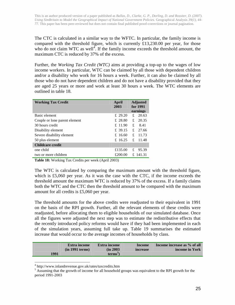
apply to all households, whether in or out of work.3 In particular, CTC can be claimed by
all persons who are responsible for at least one child under 16 years of age or under 19
years and in full-time non-advanced education. CTC comprises 5 elements which are
listed in table 17.
Elements of Child Tax Credit Amount in April 2003 Adjusted to 1991 prices
Family element £10.45 £ 7.38
Family element baby addition £10.45 £ 7.38
Child element £27.75 £19.61
Disabled child element £41.30 £29.18
Enhanced Disabled Child Element £16.60 £11.73
Table 17: Child Tax Credits, weekly (April 2003)
3 Inland Revenue web-site: http://www.inlandrevenue.gov.uk/taxcredits/changes.htm#ctc
This is an author produced version of a paper published as Ballas, D., Clarke, G. P., Dorling, D. and Rossiter, D. (2007).
Using SimBritain to Model the Geographical Impact of National Government Policies. Geographical Analysis 39(1), 44-
77. This paper has been peer-reviewed but does not contain final published proof-corrections or journal pagination.
25
The CTC is calculated in a similar way to the WFTC. In particular, the family income is
compared with the threshold figure, which is currently £13,230.00 per year, for those
who do not claim WTC as well4. If the family income exceeds the threshold amount, the
maximum CTC is reduced by 37% of the excess.
Further, the Working Tax Credit (WTC) aims at providing a top-up to the wages of low
income workers. In particular, WTC can be claimed by all those with dependent children
and/or a disability who work for 16 hours a week. Further, it can also be claimed by all
those who do not have dependent children and do not have a disability provided that they
are aged 25 years or more and work at least 30 hours a week. The WTC elements are
outlined in table 18.
Working Tax Credit April
2003
Adjusted
for 1991
earnings
Basic element £ 29.20 £ 20.63
Couple or lone parent element £ 28.80 £ 20.35
30 hours credit £ 11.90 £ 8.41
Disability element £ 39.15 £ 27.66
Severe disability element £ 16.60 £ 11.73
50 plus element £ 16.25 £ 11.48
Childcare credit
one child £135.00 £ 95.39
two or more children £200.00 £ 141.31
Table 18: Working Tax Credits per week (April 2003)
The WTC is calculated by comparing the maximum amount with the threshold figure,
which is £5,060 per year. As it was the case with the CTC, if the income exceeds the
threshold amount the maximum WTC is reduced by 37% of the excess. If a family claims
both the WTC and the CTC then the threshold amount to be compared with the maximum
amount for all credits is £5,060 per year.
The threshold amounts for the above credits were readjusted to their equivalent in 1991
on the basis of the RPI growth. Further, all the relevant elements of these credits were
readjusted, before allocating them to eligible households of our simulated database. Once
all the figures were adjusted the next step was to estimate the redistributive effects that
the recently introduced policy reforms would have if they had been implemented in each
of the simulation years, assuming full take up. Table 19 summarises the estimated
increase that would occur to the average incomes of households by class.
1991
Extra income
(in 1991 terms)
Extra income
(in 2003
terms5)
Income
increase
Income increase as % of all
income in York
4 http://www.inlandrevenue.gov.uk/rates/taxcredits.htm
5 Assuming that the growth of income for all household groups was equivalent to the RPI growth for the
period 1991-2003

This is an author produced version of a paper published as Ballas, D., Clarke, G. P., Dorling, D. and Rossiter, D. (2007).
Using SimBritain to Model the Geographical Impact of National Government Policies. Geographical Analysis 39(1), 44-
77. This paper has been peer-reviewed but does not contain final published proof-corrections or journal pagination.
26
Very poor £10,365,947 £13,403,169 34.1% 1.90%
Poor £ 5,199,802 £ 6,723,344 10.02% 0.95%
Below-average £ 4,911,779 £ 6,350,931 7.82% 0.90%
Above-average £ 2,454,956 £ 3,174,258 3.59% 0.45%
Affluent £ 5,627,831 £ 7,276,785 0.71% 1.03%
2001
Very poor £10,689,087 £13,820,989 29.3% 1.64%
Poor £ 6,511,030 £ 8,418,761 9.07% 1.00%
Below-average £ 4,169,833 £ 5,391,595 6.62% 0.00%
Above-average £ 4,570,505 £ 5,909,663 5.00% 0.00%
Affluent £ 1,626,691 £ 2,103,311 0.44% 0.00%
2011
Very poor £11,173,514 £14,447,353 26.0% 1.46%
Poor £ 8,108,874 £10,484,774 11.05% 1.06%
Below-average £7,747,491 £10,017,506 10.52% 1.01%
Above-average £ 3,945,88 £ 5,102,034 3.27% 0.52%
Affluent £ 1,326,213 £ 1,714,794 0.29% 0.17%
2021
Very poor £16,409,094 £21,216,959 27.15% 1.99%
Poor £ 5,904,514 £ 7,634,537 11.35% 0.72%
Below-average £11,121,892 £14,380,607 4.90% 1.35%
Above-average £ 4,661,651 £ 6,027,515 2.65% 0.57%
Affluent £ 787,554 £ 1,018,308 0.19% 0.10%
Table 19: Simulated impact of April 2003 policy changes by household class and simulation year.
The new tax credits would result in a more significant increase of the average income of
the poor and very poor households. For instance, in 1991 the increase of the income of
the very poor households is estimated to more than double with the implementation of the
new tax credits, compared to the trend-based increase presented in section 4.1. Similar
differences can be observed in all of the simulation years. These large differences may be
explained by the fact that the child tax credits can be claimed by unemployed individuals
with children. Further, it should be noted that the working tax credit can be claimed by
individuals in poor households without children, whereas the previous credits under
WFTC were only aimed at households with dependent children.
6 Estimating small-area impacts
The analysis presented so far is geographical in the sense that it describes the quality of
life of households at the metropolitan district level (York). In particular, we have
presented the results of the application of SimBritain for the city of York. Clearly, this
analysis can be extended to include all districts in Britain and map socio-economic
patterns across British regions and districts.
Nevertheless, it is also possible to use spatial microsimulation models to examine the
impact of policy changes at the intra-district level. This section presents the geographical
distribution of the simulated policy impacts within York. Figure 6 depicts the spatial
distribution of the average additional household income which would result from the
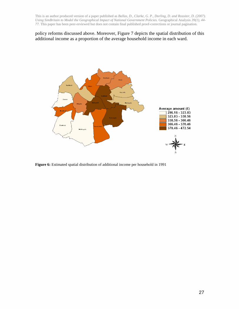
This is an author produced version of a paper published as Ballas, D., Clarke, G. P., Dorling, D. and Rossiter, D. (2007).
Using SimBritain to Model the Geographical Impact of National Government Policies. Geographical Analysis 39(1), 44-
77. This paper has been peer-reviewed but does not contain final published proof-corrections or journal pagination.
27
policy reforms discussed above. Moreover, Figure 7 depicts the spatial distribution of this
additional income as a proportion of the average household income in each ward.
Figure 6: Estimated spatial distribution of additional income per household in 1991
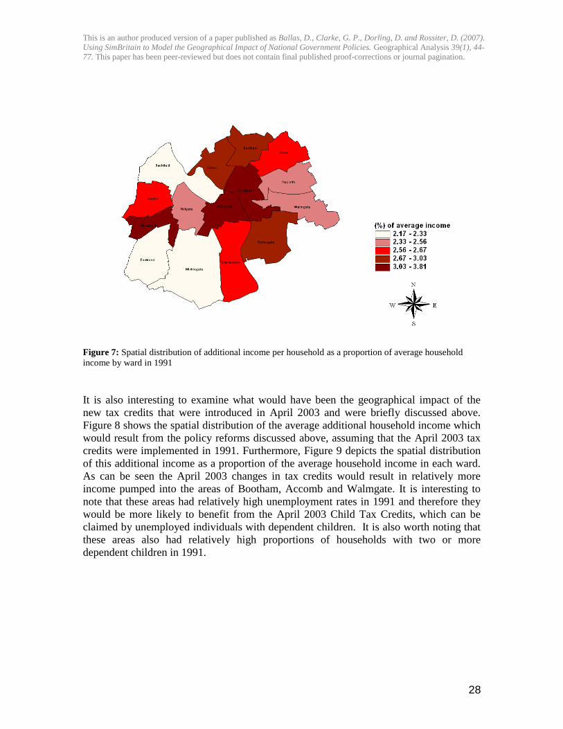
This is an author produced version of a paper published as Ballas, D., Clarke, G. P., Dorling, D. and Rossiter, D. (2007).
Using SimBritain to Model the Geographical Impact of National Government Policies. Geographical Analysis 39(1), 44-
77. This paper has been peer-reviewed but does not contain final published proof-corrections or journal pagination.
28
Figure 7: Spatial distribution of additional income per household as a proportion of average household
income by ward in 1991
It is also interesting to examine what would have been the geographical impact of the
new tax credits that were introduced in April 2003 and were briefly discussed above.
Figure 8 shows the spatial distribution of the average additional household income which
would result from the policy reforms discussed above, assuming that the April 2003 tax
credits were implemented in 1991. Furthermore, Figure 9 depicts the spatial distribution
of this additional income as a proportion of the average household income in each ward.
As can be seen the April 2003 changes in tax credits would result in relatively more
income pumped into the areas of Bootham, Accomb and Walmgate. It is interesting to
note that these areas had relatively high unemployment rates in 1991 and therefore they
would be more likely to benefit from the April 2003 Child Tax Credits, which can be
claimed by unemployed individuals with dependent children. It is also worth noting that
these areas also had relatively high proportions of households with two or more
dependent children in 1991.
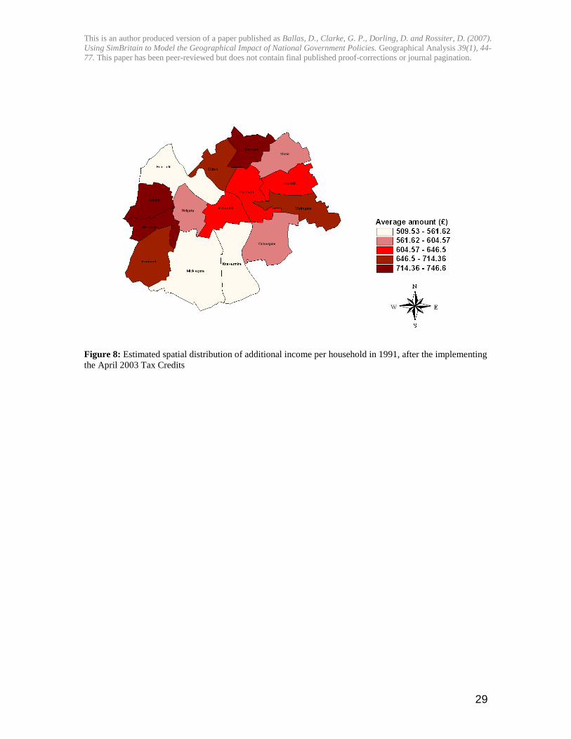
This is an author produced version of a paper published as Ballas, D., Clarke, G. P., Dorling, D. and Rossiter, D. (2007).
Using SimBritain to Model the Geographical Impact of National Government Policies. Geographical Analysis 39(1), 44-
77. This paper has been peer-reviewed but does not contain final published proof-corrections or journal pagination.
29
Figure 8: Estimated spatial distribution of additional income per household in 1991, after the implementing
the April 2003 Tax Credits

This is an author produced version of a paper published as Ballas, D., Clarke, G. P., Dorling, D. and Rossiter, D. (2007).
Using SimBritain to Model the Geographical Impact of National Government Policies. Geographical Analysis 39(1), 44-
77. This paper has been peer-reviewed but does not contain final published proof-corrections or journal pagination.
30
Figure 9: Spatial distribution of additional income per household as a proportion of average household
income by ward, after the implementation of the April 2003 Tax Credits
7. Concluding comments
The research presented here aims at building a national dynamic spatial microsimulation
model of Britain (SimBritain), that would be capable of simulating the changing
population of the whole of Britain into the future, first under the assumption that it
continues to change as it has and then under different scenarios. It should be noted that
the SimBritain model is the first of its kind and there is a lot of potential for further
improvement. It is useful at this stage to outline the ways in which the model, in its
current form, can or cannot be used.
SimBritain can be used to paint a picture of one possible future of a city or region, based
on past trends. This is demonstrated in this paper that showed how the model has been
used to paint a picture of York, in which there is near full employment and polarization is
determined largely by educational qualifications with fewer poor people but more poor
children (this is the picture the default simulation produces.) SimBritain is also suitable
for the estimation of variables such as household income at the small area level. Such
estimations can provide helpful insights into the analysis of spatial and socio-economic
polarisation within cities. SimBritain can also be used to paint a picture of the life of
households of different income categories. In this respect, the SimBritain outputs are very
similar to large-scale survey outputs and qualitative research findings. SimBritain is
useful in modelling the socio-economic and spatial effects of policy change.

This is an author produced version of a paper published as Ballas, D., Clarke, G. P., Dorling, D. and Rossiter, D. (2007).
Using SimBritain to Model the Geographical Impact of National Government Policies. Geographical Analysis 39(1), 44-
77. This paper has been peer-reviewed but does not contain final published proof-corrections or journal pagination.
31
Overall, tools such as the SimBritain model can be used to provide useful information on
socio-economic trends, as well as on the possible outcome of policy reforms, at different
geographical scales. It can be argued that the analyses presented in this paper can
stimulate debate about the future and, possibly, the future educational divide.
Nevertheless, as can be seen by the sensitivity analysis, SimBritain performs better at the
metropolitan district and parliamentary constituency level, rather than the ward level. It is
therefore more suitable for the prediction of a wide range of socio-economic variables at
the coarser geographical level of cities and regions, but it is less suitable to analyse most
variables at small area levels such as wards and enumeration districts. SimBritain is thus
also not suitable for the prediction of rare or badly reported events, such as drug use.
Also, it is unsuitable for the prediction of variables that are affected considerably by
external and localised factors, such as transport networks and public transport services.
As noted above, SimBritain has been used in this paper to provide estimates of the
redistributive impacts of some of the policy changes that occurred within the last 10
years. The findings show a situation where the natural dynamics show a more polarised
population in terms of income and wealth. In that sense these results back up more
qualitative studies such as those by Bradshaw (2000), Dorling and Tomaney (1995),
Dorling and Woodward (1996) and Walker (1999). Thus, the estimation of the impacts of
changing social policy is crucially important if we are to offer our future children a
decent standard of living.
References Ballas, D. (2001), A spatial microsimulation approach to local labour market policy
analysis, unpublished PhD thesis, School of Geography, University of Leeds
Ballas, D., Clarke, G.P., Dorling, D., Eyre, H. and Rossiter, D., Thomas, B (2005a)
SimBritain: a spatial microsimulation approach to population dynamics, Population,
Place and Space, vol. 11, pp. 13-34
Ballas, D., Clarke, G.P., Wiemers, E. (2005b), Building a dynamic spatial
microsimulation model for the Irish Rural Economy, Population, Space and Place, 11,
157–172
Bertuglia, C.S., Clarke, G.P. and Wilson, A.G. (1994) „Models and performance
indicators in urban planning: the changing policy context‟, in C.S. Bertuglia, G.P.
Clarke and A.G. Wilson (eds) Modelling the City. London: Routledge, pp. 20–36
Birkin, M., Clarke, M. (1988), SYNTHESIS – a synthetic spatial information system for
urban and regional analysis: methods and examples, Environment and Planning A, 20,
1645-1671
Birkin, M., Clarke, M. (1989), The generation of individual and household incomes at the
small area level using Synthesis, Regional Studies, 23, 535-548
Birkin, M., Clarke G.P., Clarke, M. (1996), Urban and regional modelling at the
microscale, in G.P. Clarke (ed.) Microsimulation for Urban and Regional Policy
Analysis, Pion, London, 10-27
Bradshaw, J. (2000), Prospects for poverty in the first 25 years of the next millennium,
Sociology, vol.34, pp. 1-18
This is an author produced version of a paper published as Ballas, D., Clarke, G. P., Dorling, D. and Rossiter, D. (2007).
Using SimBritain to Model the Geographical Impact of National Government Policies. Geographical Analysis 39(1), 44-
77. This paper has been peer-reviewed but does not contain final published proof-corrections or journal pagination.
32
Clarke, G.P. (1996), Microsimulation: an introduction, in G.P. Clarke (ed.),
Microsimulation for Urban and Regional Policy Analysis, Pion, London, 1-9
Clarke, G.P. & Wilson, A.G. (1994), A new geography of performance indicators for
urban planning. In C.S. Bertunglia, G.P. Clarke & A.G. Wilson (eds.), Modelling the
City, London, 55-81.
Dorling, D. and Tomaney, J. (1995) „Poverty in the old industrial regions: a comparative
view‟, in C. Philo (ed.) Off the Map: The Social Geography
of Poverty in the UK. London: Child Poverty Action Group, pp. 103–32
Dorling, D. and Woodward, R. (1996) „Social polarisation 1971–1991: a micro-
geographical analysis of Britain‟, Progress in Planning, Vol. 45, No. 2, pp. 1–67
Falkingham J, Lessof C. 1992. Playing God or LIFEMOD – The construction of a
dynamic microsimulation model. In Microsimulation Models for Public Policy
Analysis: New Frontiers, Hancock R, Sutherland H (eds). Suntory-Toyota
International Centre for Economics and Related Disciplines – LSE: London; 5-32.
Fienberg, S.E. (1970), An iterative procedure for estimation in contingency tables, Annals
of Mathematical Statistics, 41, 907-917
Fitzpatrick, P. et al. (2002) Welfare Benefits Handbook 2002/03. London: Child Poverty
Action Group
Johnston, R J, Pattie, C J (1993), Entropy-maximizing and iterative proportional fitting
procedure, Professional Geographer, 45, 317-322
Hancock, R., Sutherland, H. (eds) (1992), Microsimulation models for public policy
analysis: new frontiers, Suntory-Toyota International Centre for Economics and
Related Disciplines – LSE, London
Harding, A. (ed.) (1996) Microsimulation and Public Policy. Contributions to Economic
Analysis No. 232. Amsterdam: North Holland
Longley, P.A., Goodchild, M.F., Maguire, D.J. and Rhind, D.W. (eds) (1999)
Geographical Information Systems: Management Issues and Applications. New York:
Wiley
Martin, D. (1996), Geographic Information Systems: socioeconomic applications,
Routledge, London.
Mitton, L, Sutherland, H. and Weeks, M. (eds) (2000) Microsimulation Modelling for
Policy Analysis: Challenges and Innovations. Cambridge: Cambridge University Press
Mosteller F (1968), „Association and estimation in contingency tables‟, Journal of the
American Statistical Association, 63, 128
Norman, P. (1999), Putting Iterative Proportional Fitting on the Researcher’s Desk,
working paper 99/03, School of Geography, University of Leeds, Leeds LS2 9JT
Rogerson, P A, Plane, D A (1998), The dynamics of neighborhood age composition,
Environment and Planning A, 30, 1461-1472
Rowntree, B.S.(2000) Poverty: a study of Town Life, centenary edition, Policy Press,
Bristol
Shephard, A. (2003) Inequality under Government. Briefing Note 33. London: Institute
for Fiscal Studies
Stillwell, J. and Scholten, H. (eds) (2001) Land Use Simulation for Europe. Dordrecht:
Kluwer
Survey User Manual Volume A: Introduction,Technical Report and Appendices.
Colchester: University of Essex

This is an author produced version of a paper published as Ballas, D., Clarke, G. P., Dorling, D. and Rossiter, D. (2007).
Using SimBritain to Model the Geographical Impact of National Government Policies. Geographical Analysis 39(1), 44-
77. This paper has been peer-reviewed but does not contain final published proof-corrections or journal pagination.
33
Sutherland, H. and Piachaud, D. (2001) „Reducing child poverty in Britain: an assessment
of government policy 1997–2001‟, The Economic Journal, Vol. 111, pp. 85–101
Taylor, M.F. (ed). with Brice, J., Buck, N. and Prentice-Lane, E. (2001) British
Household Panel
Van Immoff E., Post W. (1998) Microsimulation methods for population projection,
Population: an English Selection, 10(1), 97-138
Walker, R. (1999), Ending child poverty: popular welfare for the 21st century?, Policy
Press, Bristol.
Williamson, P., Birkin, M., Rees, P. (1998), The estimation of population microdata by
using data from small area statistics and samples of anonymised records, Environment
and Planning A, 30, 785-816
Wong, D.W.S. (1992), The Reliability of Using the Iterative Proportional Fitting
Procedure, Professional Geographer, 44, 340-348

This is an author produced version of a paper published as Ballas, D., Clarke, G. P., Dorling, D. and Rossiter, D. (2007).
Using SimBritain to Model the Geographical Impact of National Government Policies. Geographical Analysis 39(1), 44-
77. This paper has been peer-reviewed but does not contain final published proof-corrections or journal pagination.
34
Appendix
BHPS Individual Questionnaire
Core Neighbourhood and individual:
Demographics
Birthplace, Residence Satisfaction with
Home/Neighbourhood
Reasons for Moving Ethnicity
Educational background
and attainments
Recent Education/Training
Partisan support
Changes in marital status Citizenship
Current Employment: Employment status
Not working/Seeking work
Self Employed Sector Private/Public
SIC/SOC/ISCO
Nature of Business/Duties Workplace/Size of Firm
Travelling Time
Means of Travel
Length of Tenure
Hours worked/Overtime
Union Membership Prospects/Training/Ambitions
Superannuation/Pensions
Attitudes to work/Incentives Wages/Salary/Deductions
Childcare provisions
Job search activity Career Opportunities
Bonuses
Performance related pay
Finances: Incomes from:
Benefits/Allowances/Pensions/Rents/Savings/ Interest/Dividends
Pension Plans Savings and Investments
Material well-being
Consumer Confidence
Internal Transfers
External Transfers
Personal Spending Roles of partners/Spouses
Domestic work/Childcare/Bills/Everyday
Spending Car Ownership/Use/Value of Car
Interview Characteristics
Windfalls
Rotating
Core
Health and Caring:
Personal health condition
Employment constraints Visits to doctor
Hospital/Clinic use
Use of Health/Welfare Services
Social Services
Specialists Check-ups/Tests/Screening
Smoking
Caring for relatives/others Time spent caring for
others
Private medical insurance Activities in daily living
Employment History:
Past year
Labour Force Status Spells Size/Sector/Nature of
Business/Duties
Wages/Salary/Deductions Reasons for leaving/taking
jobs
Values and Opinions:
Partisanship/Interest in Politics
Religious Involvement Parental Questionnaire
Variable
Components
Lifetime Marital Status
History (Wave 2): Number of marriages
Marriage dates
Divorce/widowhood/ Separation dates
Cohabitation before
marriage
Lifetime Marital Status
History (Wave 3): Start and finish dates
Labour force status
Sector/nature of business duties
Lifetime Fertility and Adoption
History (Wave 2 and Wave 8 catch-up):
Birth dates
Adoption dates Sex of children
Leaving or mortality dates
Lifetime Cohabitation History
(Wave 2 and Wave 8 catch-up):
Start and finish dates Number of partners
Lifetime Employment Status History(Wave 2):
Start and finish dates Employment status
Values and Opinions: Aspirations for children
Important Events
Quality of Life
Credit and Debt:
Investment and Savings Commitments
Appendix: Details of the core, rotating core and variable component question subject areas from the BHPS
Individual Questionnaire (from: Taylor et al., 2001).