Using Remote Sensing Data to Study Wetland

Dynamics in Iowa

Principal Investigator: Dr. Ramanathan Sugumaran

Graduate Students: James Harken & James Gerjevic Department of Geography

University of Northern Iowa Cedar Falls, IA - 50614

Iowa Space Grant (Seed) Final Technical Report January 2004

2

Using Remote Sensing Data to Study Wetland Dynamics in Iowa ABSTRACT

Wetlands are transitional lands between terrestrial and aquatic systems that provide many

goods and services, including flood water retention, water quality maintenance, wildlife habitat, and soil erosion control. Wetlands in Iowa have decreased over 95% in the last 200 years. The loss of these resources and benefits shows a need to map and monitor wetlands in Iowa, especially where current wetland maps are outdated, as is the case in Black Hawk County. Traditional wetland ground surveys are too time consuming and expensive though, and remote sensing imagery can provide time and cost-effective solutions. This study tests the feasibility of using high resolution airborne Color Infrared (CIR) imagery, multi-spectral hybrid data, and high resolution hyper-spectral imagery to map and monitor wetlands in Iowa. In addition, this project compares traditional classifiers with an object-oriented (OO) classification technique to improve wetland mapping accuracy. Wetlands in Black Hawk County showed a slight decrease of roughly 1500 acres (+/- an error margin of 375 acres) from 1983-2003. In general, the OO classifier performed better than traditional pixel-based techniques (Maximum Likelihood and ISODATA) for the CIR and Landsat imagery and better than the Spectral Angle Mapper (SAM) technique for the hyperspectral image. Finally, a Web-based tool was developed using ArcIMS to disseminate the data developed from this study to stakeholders. INTRODUCTION

Cowardin et al. (1979) provides the official federal definition of wetlands: “Wetlands are lands transitional between terrestrial and aquatic systems where the water table is usually at or near the surface or the land is covered by shallow water”. Other definitions include “a mix of characteristics from terrestrial or upland areas and the characteristics of aquatic or water environments” (Lyon, 1993), and “places where plants and animals live amid standing water or saturated soils, also called swamps, sloughs, marshes, bogs, fens, seeps, oxbows, shallow ponds, or wet meadows” (IDALS, 1998). The US Army Corp of Engineers Wetlands Delineation manual (1987) defines wetlands as “Those areas that are inundated or saturated by surface or ground water at a frequency and duration sufficient to support and that under normal circumstances do support, a prevalence of vegetation typically adapted for life in saturated soil conditions”.

Wetlands compromise only three to six percent of the earth's land surface area, but they provide human populations with a host of goods and services, including water quality maintenance, agricultural production, fisheries, and recreation (Acreman & Hollis, 1996). Despite these proven advantages, wetland conversion to other land uses has been a problem historically and continues to the present day. Nationally, at the time of European settlement, the continental United States contained an estimated 221 million acres (89.5 million hectares) of wetlands. Over time, wetlands have been drained, dredged, filled, leveled, and flooded to the extent that less than half of the original acreage remains (Dahl, 1990, Whittecar & Daniels, 1999). Within the state of Iowa, wetlands were viewed as a hindrance to land development and agriculture. In less than 150 years, these rich resources were drained, filled, or otherwise altered, drastically changing the face of Iowa's land. Conflicting percentages are given concerning the amount of wetland losses in Iowa. One study states 95% (Arbuckle & Pease, 1999) and another 90%-95% (Cohen, 2001). Both however, are high, and represent the majority of pre-European settlement Iowa wetlands. In a mandated report to Congress by the US Fish and Wildlife Service, only two other states showed higher wetlands losses than Iowa, California and Ohio (Dahl, 1990). And according to the USGS (IDALS, 1998) the amount of wetlands six years ago covered only 1.2% of Iowa’s surface area, compared to 11% 200 years ago. The reduction of wetlands in Iowa also contributes to the fact that Black Hawk, Hamilton, Johnson, Linn, Story, and Tama counties were designated federal (flood) disasters five times from 1989-

3

1998 (Sierra Club, 2000) and all of Iowa's 99 counties were designated federal (flood) disaster areas at least once in that time.

The loss of these critical resources (wetlands) in Iowa with some 92% of the land being used for agriculture, and their documented value of storing floodwaters, maintaining water quality, lessening soil erosion, and providing wildlife habitat, shows an urgent need for mapping and monitoring theses resources, as well as determining potential restoration areas. Traditionally, wetlands are delineated using ground surveys. However, the surveys are difficult and time-consuming (Yasouka et al., 1995; Lyon, 1993). Remote sensing is one of the technologies that can provide cost and time-effective solutions to mitigate these problems (Goldberg, 1998). In addition, remote sensing technologies can supply the following information: (1) extent of wetlands, (2) identify the wetland resource as to type, (3) characterize the general wetland land cover type, (4) identify submergent and emergent wetlands, and (5) supply details about the resource using multiple spectral analysis of remote sensor data (Lyon & McCarthy, 1995). The following sections briefly describe the literature review for multispectral, hyperspectral image classifications and also object oriented method for wetland mapping and monitoring. Literature Review: Multi-Spectral Classification of Wetlands

Traditionally, Landsat MSS, Landsat TM, and SPOT satellite systems have been used to study

wetlands (Lunetta & Balogh, 1999; Shaikh et al., 2001; Shepherd et al., 2000; Töyrä et al., 2000). Other studies have included AVHRR, IRS, JERS-1, ERS-1, SIR-C and RADARSAT (Alsdorf et al., 2001; Bourgeau-Chavez et al., 2001; Chopra et al., 2001). There are limitations in delineating wetlands using traditional, optical, multi-spectral techniques. One limitation on the use of optical data for wetland mapping is their inability to penetrate vegetation canopies, and thus their inability to remotely sense flooding beneath a closed canopy (Bourgeau-Chavez et al., 2001). There has been some research done on wetlands using radar data (Bourgeau-Chavez et al., 2001; Alsdorf et al., 2001; Rio & Lozano-García, 2000) as well as LIDAR (MacKinnon, 2001) but the majority has been concentrated on Landsat TM, MSS, SPOT, and airborne CIR photos.

As far as classification of these images is concerned, most of the earliest work included visual interpretation of aerial photographs. Unsupervised classification or clustering is the most commonly used digital classification to map wetlands and the Maximum Likelihood algorithm with a supervised method (Özemi, 2000). Low wetland accuracy percentages usually accompany these classification methods (30 – 60% accuracies). Several researchers increased the accuracy with other methods, for example, using multi-temporal and ancillary data along with various GIS models and non-parametric classifiers such rule-based classifiers (using multi-spectral imagery) (Özemi, 2000). Hodgson et al., (1987) also indicated wetlands could be better defined on imagery acquired in spring when the water table was high. Other work has been done using multi-sensor assessment (Töyrä et al., 2001), neural networks (Han et al., 2003; Özemi, 2000), hyperspectral data (Schmidt & Skidmore, 2003) and ancillary data (Houhoulis & Michener, 2000). Ancillary data provides a practical solution to help the problem of distinguishing between spectral similarities in wetlands, agricultural fields, and forests (Houhoulis & Michener, 2000). Object Oriented Classification of Wetlands

In contrast to traditional image processing methods, the basic processing units of object oriented analysis are image objects or segments, and not single pixels (Baatz & Schape, 2001). The reasoning behind this is the expected result of many image analysis tasks is the extraction of real world objects. Representation of image information is based on the networking of these image objects, which must be explicitly worked out in contrast to implicit neighbor objects on the pixel scale. Scale is an important consideration in object oriented analysis because it determines the occurrence or nonoccurrence of a certain object class, i.e. a house or a subdivision, or a field or an ecosystem. This is achieved by a strict hierarchical structure that allows relations between objects and their sub-objects and super-objects. Single pixel objects

4

represent the smallest possible processing scale. Other information used in OOA includes tone, shape, texture, context, and information from other object layers.

Object-oriented classification is relatively new to the field of remote sensing and most of the studies done have taken advantage of high-resolution imagery (IKONOS, etc.) for land cover classification. Of particular interest to many researchers is urban classification due to the form, size and neighborhood functions associated with eCognition software. However, this does not exclude land cover (and wetland) classification, as shown by the studies Gomes & Marcal (2003); Antunes et al., (2003); Kaya et al., (2002); Civco et al., (2002); and Ivits & Koch (2000). Gomes & Marcal (2003) used 9 band 15 m ASTER imagery to revise a 1995 land cover data set for the Vale do Sousa region in northwest Portugal. Their overall accuracy was 71.5% and forested areas (which were emphasized in the study) had an average accuracy of 46.3%. Antunes et al. (2003) segmented a 4 band IKONOS image to identify riparian (wetland) areas that could not be spectrally differentiated in the northern part of the state of Parana in Brazil. They needed to map declining wetland areas for resource management because of increased agricultural activities. Their accuracies were 75.4% for riparian vegetation and 78.6% for swamp vegetation. They also ran a Bayesian Maximum Likelihood classifier for the same areas and came up with 56.0% for riparian areas and 45.3% for swamp vegetation. Although they showed promising results, there was a disappointing lack of detail in their exact pre-processing and methodology steps. Civco et al., (2002) compared knowledge-based and object-oriented techniques (among others) for land cover change detection in the Stony Brook Millstone River watershed in New Jersey using Landsat ETM+ data. They concluded that no single method was superior (from knowledge-based, object-oriented, neural networks, and traditional techniques) for their study data and area. However, they reported that “image segmentation and object-oriented classification holds much promise” and “appeared to have produced better overall results, especially in terms not only detecting and characterizing the nature of change, but also in minimizing the salt-and-pepper effect caused by isolated and non-contiguous pixels”. Ivits & Koch (2000) used six European test sites and IRS panchromatic and Landsat ETM imagery along with object-oriented classification to develop a preliminary landscape habitat ecological analysis.

Hyperspectral Classification of Wetlands

Hyperspectral classification of wetlands is relatively new and the literature is not yet fully developed. Relevant studies include Anderson et al., 2003; Juan et al., 2000; Bakker & Schmidt, 2002; Schmidt & Skidmore, 2002; and the Wetlands Reserve Program, 1994. Schmidt and Skidmore (2003) studied 27 salt marsh vegetation types in a coastal Dutch wetland and concluded that statistical variation of wetland vegetation reflectance spectra is possible in the visible to short-wave range. They used a three step analysis to test difference between type classes, used continuum removal as a normalization technique in the visible range (although it failed in the infrared range), and measured the distance of the vegetation types in spectral space using the Bhattacharyya and Jeffries-Matusita distance measures. S-Plus software was used to process the 579 bands between 400 and 2500 nm with a gap between 1820 to 1940 nm for atmospheric water absorption. A GER spectrometer was used to measure the in situ reflectance on 132 vegetation plots. The bands found to be the most useful for discriminating wetland vegetation types were between 740-1820 nm in the shortwave infrared and between 400 to 700 nm in the visible spectrum. Six wavelength bands were then selected out of the above mentioned bands based on their higher frequency of statistically different median reflectance and there more-or-less spacing across the whole spectrum. Those bands are: 404, 628, 771, 1398, 1803, and 2183 nm. This study provides a foundation for other researchers wishing to test those specific bands for their own wetland study areas. The Wetlands Reserve Program Technical Note used NASA’s AVRIS sensor to test hyperspectral feasibility for wetlands mapping in Green Bay, Wisconsin. Unfortunately, only the spectral signatures were collected and no further analysis was done. Bakker and Schmidt (2003) concentrate on edge filtering for hyperspectral images in agriculture and salt marsh test areas. They conclude that hyperspectral edge filters can assist in image interpretations. Lastly, Juan et al., (2000) flew a

5

hyperspectral mission over Fort Drum Marsh in Florida using an unspecified hyperspectral sensor that collected 64 wavebands in the 399.2 to 920.5 nm range. They were successful in delineating the wetland species from the airborne hyperspectral imagery but did not release what wavebands were most sensitive for different plant species.

GOALS AND OBJECTIVES

The main research goal was to study wetland mapping and monitoring using remote sensing data in Iowa. To achieve this goal, the following four objectives were presented:

1) Investigate the potential use of 1 meter Color Infrared (CIR) 2002 photographs and

hybrid data (pan-sharpened and multi-seasonal multispectral Landsat ETM+) data in wetland delineation;

2) Evaluate different image classifiers, specifically Object-oriented, Maximum-Likelihood and Spectral Angle Mapper;

3) Monitor wetland dynamics for Black Hawk County using 1983 National Wetlands Inventory data and a current 2003 wetlands map created from objectives 1 and 2;

4) Creation of a web-based tool to allow dissemination of data developed from the above objectives.

MATERIALS AND METHODS Study Area and Data Used Mulitspectral Images:

Black Hawk County, Iowa is the fourth most populous county in the state and is located at

42.491N Latitude and -92.367W Longitude. The multispectral imagery used for classification is as follows: An April 2002 1 meter resolution Color Infrared Photo mosaic (Figure 1), obtained from the Iowa Geographic Image Server, a September 2000 30 m Landsat ETM+, and a July 1999 30 m Landsat ETM+ obtained from the University of Northern Iowa’s STORM Project (Figure 1). Two hybrid data sets were created by pan-sharpening the Landsat images with their 15 m panchromatic band and Principal Components Analysis and a Matrix of the two seasonal Landsat images. The choice of the data sets comes from their no cost availability and their temporal applicability (all three within the last four years). This is pertinent because of one of the project goals was to create an updated wetlands map for the county, using the most up-to-date imagery available. As stated previously, the current wetlands map, created by the Iowa DNR and National Wetlands Inventory is based on aerial photograph interpretation and field surveys done almost twenty years ago. The vector ancillary data (NWI, hydrology, soils, and conservation areas) was obtained from various sources, including the USGS, NRCS, IDNR, NWI, and Iowa Geographic Map Server. Additionally, data was acquired from the Black Hawk County GIS office. The software used was ERDAS Imagine 8.6 and eCognition 4.0.

6

Figure 1: 1 m CIR Image (left) and 15 m Landsat ETM+ image (right) of Black Hawk County, Iowa

Hyperspectral Image

Eddyville, Iowa is a small town located in the southeast part of the state along the Des Moines River at 41.160N Latitude and -92.631W Longitude. The hyperspectral imagery used for classification was flown with the CASI sensor in July of 2001 for a NCRST project (NCRST, 2002). The 2001 image is a mosaic of seven flight lines and has a spatial resolution of 60 cm with 48 contiguous spectral bands, each of which is approximately 0.018 micrometers with a range of 350 to approximately 2500 nanometers (Figure 2). In addition, a 1 meter Color Infrared Image from the Iowa DNR, digital SSURGO soil maps and National Wetlands Inventory data were used for training and accuracy assessment. The software used to process and classify the hyperspectral image was ENVI 3.6 and eCognition 4.0.

The 60 centimeter 2001 Eddyville image encompasses approximately 969 acres and contains unique ecological habitats, as discovered by the Iowa Department of Transportation when a highway bypass was begun northeast of the city until town citizens informed the IDOT of the protected species and habitats (NCRST, 2002). Upland and wetland vascular plant species in the area include: Festuca rubra L. (red fescue), Pycnanthemum tenuifolium (Slender mountain mint), Helianthus annus (sunflower), Polygonum persicaria (Spotted ladysthumb), Conyza sp., Phalaris arundinacea (Reed canarygrass), Galium aparine (Goose-grass), Utica dioica (nettles), and Morus alba (White mulberry). All of the before mentioned species occur on the 1996 National List of Vascular Plant Species that Occur in Wetlands, published by the US Fish and Wildlife Service (USFWS, 1996).

Figure 2: Hyperspectral image (A portion of study area) (Source: NCRST, 2002)

7

Image Analysis & Classification Figure 3 shows the overall multispectral processing for both the CIR and Landsat ETM+ data. Multispectral CIR Image Classification:

The unsupervised classification of the CIR 1 meter (4.6 GB file size) was completed using ERDAS Imagine’s ISODATA algorithm with the following parameters: 120 classes with a convergence threshold of .95 and 30 maximum iterations. 120 classes were selected to identify separable clusters in the histogram. Classes were then identified by visual interpretation based on the original False-Color Image and grouped and recoded into 6 general classes based on the Anderson et al. (1976) USGS classification system, Wetland, Mixed Forest, Impervious Surface, Fallow/Bare Soil, and Urban Grasses (includes Mixed and Herbaceous Grasses), and Open Water. The supervised classification of the CIR was completed with ERDAS Imagine’s Maximum Likelihood Classifier, using a created signature file of polygon AOI’s by visual interpretation and grouped into the same six general classes used in the unsupervised classification: Wetland, Mixed Forest, Impervious Surface, Fallow/Bare Soil and Mixed Grasses (includes urban and herbaceous grasses) and Open Water. The Accuracy Assessment for the CIR was performed by generating 300 random stratified points, or 50 points per class. The points were then visually interpreted on an unclassified 2002 CIR image. Multispectral ETM Image Classification:

The unsupervised classification of the Landsat ETM+ 15 m image of Black Hawk County was done using the same parameters as the other unsupervised classification (CIR) to insure statistically comparable results. The ISODATA algorithm was used to separate the image into 120 classes with a convergence of 0.95 and 20 maximum iterations. Classes were identified by visual interpretation, histogram separability, and ancillary data and then grouped into seven classes. An extra class of row crop was added to this classification because the image was captured in September and much more planted vegetation was inherent than in the April CIR. The other six classes remained the same. The supervised classification of the Landsat image was completed using the ERDAS’ Maximum Likelihood Classifier, using a created signature file of polygon AOI’s based on ground-truth points, visual interpretation, and NWI ancillary data and grouped into the same seven classes as the Supervised ASTER and Unsupervised Landsat classifications. The accuracy assessment was performed by generating 350 random stratified points (50 per class) and visually interpreted using both an aerial photo and an unclassified TM image. 5 points had to be discarded since they fell out of range.

For the Object-Oriented Classifier in eCognition, Layers 3, 4 and 5 on the Landsat Image as well as layer 3 (SWIR) on the CIR were given slightly higher weightings (1.0 compared to 0.8) during the initial segmentation based on their proven vegetation sensitivity characteristics. Each data set in eCognition was classified according to an average of 185 objects per class and 50 samples per class were tested (7 classes) for a total of 350 random sample points for the accuracy assessment (except for the Landsat ETM 30 m where lack of objects kept the points down to 20 per class). Objects generally ranged from 5-15 pixels in size for the CIR and 94-95 pixels for the Landsat image. Please refer to Figure 3 for an overall flow of the multispectral processing and classification.

The seasonal matrix (summer/fall images) was created in ERDAS Imagine’s interpreter function under GIS analysis and followed the same classification and accuracy assessment procedures as mentioned above.

8

Figure 3: Multispectral Processing Flowchart Hyperspectral Image Classification:

Figure 4 is a representation of the overall image processing flow. A MNF (Minimum Noise Fraction) algorithm was run in ENVI 3.6 to determine which bands to select. The MNF transform as modified from Green et al. (1988) and implemented in ENVI, and is essentially two cascaded Principal Component’s transformations. The first transformation, based on an estimated noise covariance matrix, decorrelates and rescales the noise in the data. This first step results in transformed data in which the noise has unit variance and no band-to-band correlations. The second step is a standard Principal Components transformation of the noise-whitened data. For the purposes of further spectral processing, the inherent dimensionality of the data is determined by examination of the final eigenvalues and the associated images. The data space can be divided into two parts: one part associated with large eigenvalues and coherent eigenimages, and a complementary part with near-unity eigenvalues and noise-dominated images. By using only the coherent portions, the noise is separated from the data, thus improving spectral processing results (ENVI User’s Manual, 2002). The Spectral Angle Mapper (SAM) algorithm is a physically-based spectral classifier that uses an n-dimensional angle to match pixels to a reference spectra (in this case the ROI training classes). The mathematical formula for SAM is as follows:

α = cos -1 ___ΣXY___ √Σ(X)2Σ(Y)2

Where; α = angle formed between reference spectrum and image spectrum X = image spectrum Y = reference spectrum It is relatively insensitive to illumination and albedo effects (ERDAS Spectral Analyst Guide, 2002). Initially, the angle tolerance between the pixels and the reference spectra was set to 0.10 radians, however this resulted in too many pixels being left unclassified so the tolerance was set higher to 0.15, which resulted in 100% pixel classification. 82 ground truth points were available for the image, 41 of which were used to develop training Regions of Interest (ROI’s)

Training Areas Identified Seasonal Matrix

Object-Oriented Classifier

1 m CIR 30 m Landsat ETM+ Pan

Pan-sharpened

Data Fusion

Maximum Likelihood Classifier

Final Output

Accuracy Assessment

9

and 41 of which were used to develop ROI’s for accuracy assessment purposes. Training and accuracy areas were also grown from seed pixels and manually delineated into polygons based on visual interpretation of a 1 meter Color Infrared Image along with corresponding digital SSURGO soil maps and National Wetlands Inventory data. 25 bands were selected and classified in ENVI using the Spectral Angle Mapper (SAM), and the object-oriented (OO) classifier in eCognition. Processing time for the SAM was 3.5 hours and 1.0 hours for the OO.

Figure 4: Hyperspectral Processing Flowchart

60 cm CASI Image

Training Areas Identified (ROIs)

Spectral Angle Mapper (SAM) Classifier

Accuracy Assessment

Final Output

Training Areas

Retrained

Object-Oriented Classification

Pre-Processing (Minimum Noise Fraction Algorithm)

Bands Selection

Final Output

10

RESULTS AND DISCUSSION Multispectral CIR image classification Figure 5 depicts the CIR image classification with three classifiers: ISODATA, supervised Maximum Likelihood, and Object-Oriented.

CIR – ISODATA classified

image CIR - ML

classified image CIR - OO image classified image

Figure 5: Results from Multispectral 1 m CIR image classification

In Figure 5, the pink areas represent wetlands, blue, open water, brown, bare soil, green

non-wetland forest and herbaceous cover, and black urban/artificial surface. The ISODATA unsupervised method gave the highest overall accuracy when classifying the CIR (79.2%) and determining wetland user’s accuracy (75.0%) while the Maximum likelihood classifier gave the highest wetland producer’s accuracy (75.0%) (Table1). The object-oriented classifier performed poorly, in contrast to previous studies that had used high-resolution imagery (4 m IKONOS) to identify wetlands (Antunes et al., 2003). Two possible reasons include incorrect scale parameters used in the segmentation step and poor spectral resolution. The eCognition (object-oriented) software consistently performed better the more layers present there were to segment (see Table 1). However, the 1 meter CIR was very useful as an ancillary data source and could be manually delineated, representing a cost-effective solution to agencies seeking to define wetlands from remotely sensed imagery. Multispectral Landsat ETM image classification

The object-oriented classifier outperformed the pixel-based methods (ISODATA & ML) when classifying the Landsat imagery. Overall accuracy was higher in both the 30 m (73.9%) and 15 m (90.7%) images (Table 1). However, wetland identification accuracy was only better than the pixel-based methods when spatial resolution was increased (73.7% producer’s accuracy, 66.7% user’s accuracy). Segmentation parameters were taken from previous studies (Antunes et al., 2003; Gomes & Marcal, 2003; Fisher et al., 2002; Meinel et al., 2001; Schiewe, 2001) which also used multispectral satellite imagery and reported generally similar accuracies for different land cover types using the object-oriented classifier. In Figure 6, the pink areas represent wetlands, blue, open water, brown, bare soil and row crop, green non-wetland forest and herbaceous cover, and grey urban/artificial surface.

11

ETM – ISODATA classified

image ETM - ML

classified image ETM - OO image classified image

Figure 6: Results from Multispectral 15 m Landsat ETM+ image classification

The seasonal matrix of the pan-sharpened Landsat images produced lower accuracies than

anticipated, especially for identifying wetland areas. It did however, increase accuracies for row crop cover and herbaceous grass cover. This may be due to the large amount of flooding present in the July 1999 Landsat image. Landsat imagery remains a valid choice for large scale wetlands mapping projects, especially with the added capability of the panchromatic band. Hyperspectral image classification

In Figure 7, for the SAM image, purple represents forest, blue, algae, green, open water, pink, bare soil, yellow, artificial surface, maroon, shadow, and orange, floodplain crop. In the OO image, blue is open water, light green, algae, grey, artificial surface, yellow, floodplain crop, black, shadow, green, forest, and brown, is bare soil.

CASI SAM classified image CASI OO classified image

Figure 7: Results from CASI hyperspectral image classification

12

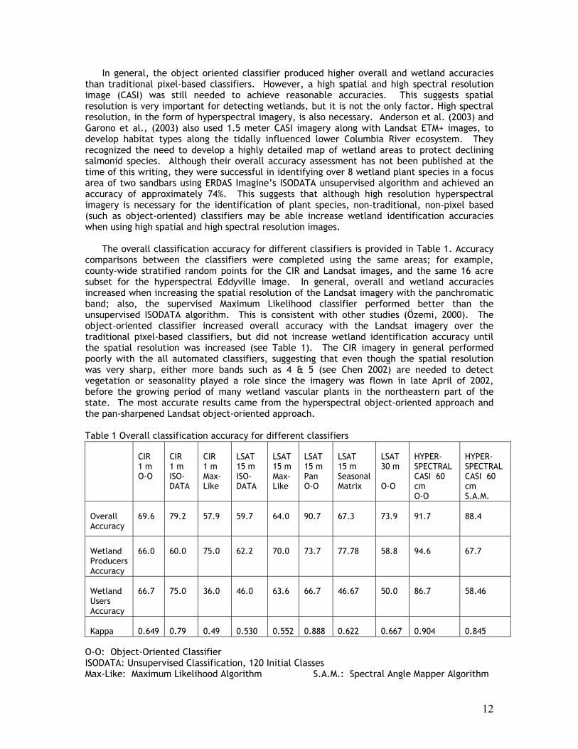
In general, the object oriented classifier produced higher overall and wetland accuracies than traditional pixel-based classifiers. However, a high spatial and high spectral resolution image (CASI) was still needed to achieve reasonable accuracies. This suggests spatial resolution is very important for detecting wetlands, but it is not the only factor. High spectral resolution, in the form of hyperspectral imagery, is also necessary. Anderson et al. (2003) and Garono et al., (2003) also used 1.5 meter CASI imagery along with Landsat ETM+ images, to develop habitat types along the tidally influenced lower Columbia River ecosystem. They recognized the need to develop a highly detailed map of wetland areas to protect declining salmonid species. Although their overall accuracy assessment has not been published at the time of this writing, they were successful in identifying over 8 wetland plant species in a focus area of two sandbars using ERDAS Imagine’s ISODATA unsupervised algorithm and achieved an accuracy of approximately 74%. This suggests that although high resolution hyperspectral imagery is necessary for the identification of plant species, non-traditional, non-pixel based (such as object-oriented) classifiers may be able increase wetland identification accuracies when using high spatial and high spectral resolution images.

The overall classification accuracy for different classifiers is provided in Table 1. Accuracy comparisons between the classifiers were completed using the same areas; for example, county-wide stratified random points for the CIR and Landsat images, and the same 16 acre subset for the hyperspectral Eddyville image. In general, overall and wetland accuracies increased when increasing the spatial resolution of the Landsat imagery with the panchromatic band; also, the supervised Maximum Likelihood classifier performed better than the unsupervised ISODATA algorithm. This is consistent with other studies (Özemi, 2000). The object-oriented classifier increased overall accuracy with the Landsat imagery over the traditional pixel-based classifiers, but did not increase wetland identification accuracy until the spatial resolution was increased (see Table 1). The CIR imagery in general performed poorly with the all automated classifiers, suggesting that even though the spatial resolution was very sharp, either more bands such as 4 & 5 (see Chen 2002) are needed to detect vegetation or seasonality played a role since the imagery was flown in late April of 2002, before the growing period of many wetland vascular plants in the northeastern part of the state. The most accurate results came from the hyperspectral object-oriented approach and the pan-sharpened Landsat object-oriented approach. Table 1 Overall classification accuracy for different classifiers

CIR 1 m O-O

CIR 1 m ISO- DATA

CIR 1 m Max- Like

LSAT 15 m ISO- DATA

LSAT 15 m Max- Like

LSAT 15 m Pan O-O

LSAT 15 m Seasonal Matrix

LSAT 30 m O-O

HYPER- SPECTRAL CASI 60 cm O-O

HYPER- SPECTRAL CASI 60 cm S.A.M.

Overall Accuracy

69.6

79.2

57.9

59.7

64.0

90.7

67.3

73.9

91.7

88.4

Wetland Producers Accuracy

66.0

60.0

75.0

62.2

70.0

73.7

77.78

58.8

94.6

67.7

Wetland Users Accuracy

66.7

75.0

36.0

46.0

63.6

66.7

46.67

50.0

86.7

58.46

Kappa

0.649

0.79

0.49

0.530

0.552

0.888

0.622

0.667

0.904

0.845

O-O: Object-Oriented Classifier ISODATA: Unsupervised Classification, 120 Initial Classes Max-Like: Maximum Likelihood Algorithm S.A.M.: Spectral Angle Mapper Algorithm

13

Monitoring Wetlands in Black Hawk County

42230

18766 17318 17257

05000

1000015000200002500030000350004000045000

1832 Source:IDNR

1983 Source:NWI

1992 Source:USGS

Landcover

2003 Source:ISGC Study

Wetland Acreage

Figure 8: Black Hawk County Wetlands Timeline

As shown by the above timeline, Figure 8, wetlands have decreased in the past twenty

years in Black Hawk County, according to the results of this study. This is possibly due to natural variations in the hydrological cycle, agricultural practices, or image bias. While the acreage amount is not great, it still shows a need for restoration planning and implementation. As Hey & Philippi (1999) note, wetlands can be restored to provide functions that have been lost. They also noted that wetland restorations are most effective when they currently occupy less than 10% of the area to be restored, as is the case in Black Hawk County where wetlands currently account for 5% of the county’s surface area. Currently we are developing a comprehensive GIS-based model that will identify which areas will provide the greatest amount of benefit for the least amount of money and area restored. Web-based data dissemination

The Black Hawk county wetland project homepage is available to the general public at http://gisrl-9.geog.uni.edu/wetland/. The homepage explains the goals and objectives and also methodologies and protocols developed in this project. Please refer to Figures 8 and 9 for a screenshot of the websites, which publishes the results of this study and also for ArcIMS based data dissemination.

Figure 8: Black Hawk County Wetland Project Home Page

14

Figure 9: A Web-based tool developed using ArcIMS http://gisrl-9.geog.uni.edu/wetland/ CONCLUSION AND FUTURE DIRECTION

In this study multispectral (CIR and ETM) and hyperspectral (CASI) images were tested for wetland classification using different classifiers (Maximum Likelihood, ISODATA, Object-Oriented and Spectral Angle Mapper). The result clearly showed that hyperspectral images produced more accurate wetland mapping than multispectral datasets when using the object-oriented classifier. Known sources of error include the fact that any wetland identified through remotely sensed imagery must be field-checked by a qualified ecologist or biologist in order to qualify for legal status or protection. Wetlands in Black Hawk County showed a slight decrease of roughly 1500 acres (+/- an error margin of 375 acres) from 1983-2003. A web site with an ArcIMS viewer was created in order to disseminate information to the stakeholders involved in the study. The future direction of this study lies in testing more non-parametric classifying methods, studying the seasonal effects particularly with hyperspectral images, and implementing a wetland restoration model for Black Hawk County using GIS.

15

REFERENCES Acreman, M.C. & Hollis, G.E. (1996) Water Management and Wetlands in Sub-Saharan Africa. IUCN,

Gland, Switzerland. Alsdorf, D.E., Smith, L.C, & Melack, J.M. (2001) Amazon Floodplain Water Level Changes Measured with

Interferometric SIR-C Radar. IEEE Transactions on Geoscience and Remote Sensing, Vol. 39, No. 2, pp. 423-431.

Anderson, B.D., Garono, R., and Robinson, R. (2003) CASI and Landsat: Developing a Spatially Linked,

Hierarchical Habitat Cover Dataset along the Lower Columbia River, USA. Retrieved December 9, 2003 from http://www.waterobserver.org/event-2003-06/pdf/paper-04-June-05-BAnderson.pdf

Anderson, J.R., Hardy, E., Roach, J.T., Witmer, R.E. (1976) A Land Use and Land Cover Classification

System For Use With Remote Sensor Data, United States Government Printing Office, Washington D.C., United States Department of the Interior

Antunes, A.Z.B., Lingnau, C., & Da Silva, J.C. (2003) Object-Oriented Analysis and Semantic Network for

High Resolution Image Classification. Anais XI SBSR, Belo Horizonte, Brasil, 05-10, abril, INPE, p. 273-279.

Arbuckle, K., & Pease, J.L. (1999) Managing Iowa Habitats: Restoring Iowa Wetlands. Iowa State

University Extension, Pm-1351h. Arbuckle, K., & Pease, J.L. (1999) Managing Iowa Habitats: Restoring Iowa Streams. Iowa State

University Extension, Pm-1351j. Baatz & Schape (2001) eCognition User’s Manual. Bakker, W.H., & Schmidt, K.S. (2002) Hyperspectral edge filtering for measuring homogeneity of surface

cover types, Photogrammetry & Remote Sensing, Vol. 56, pp. 246-256. Bourgeau-Chavez, L.L., Kasischke, E.S., Brunzell, S.M., Mudd, J.P., Smith, K.B., Frick, A.L. (2001)

Analysis of space-borne SAR data for wetland mapping in Virginia riparian ecosystems, International Journal of Remote Sensing, Vol. 22, No. 18, pp. 3665-3687.

Chen, J-H., Chun-E, K., Tan, C-H., & Shih, S-F. (2002) Use of spectral information for wetland

evapotranspiration assessment. Agricultural Water Management 55, 239-248. Chopra, R., Verma, V.K., & Sharma, P.K. (2001) Mapping, monitoring and conservation of Harike wetland

ecosystem, Punjab, India, through remote sensing, International Journal of Remote Sensing, Vol. 22, No. 1, pp. 89-98.

Civco, D.L., Hurd, J.D., Wilson, E.H., Song, M., & Zhang, Z. (2002) A Comparison of Land Use and Land

Cover Change Detection Methods, ASPRS-ACSM Annual Conference and FIG XXII Congress, April 22-26, 2002.

Cohen, D. (2001) Iowa Wetlands, Iowa Association of Naturalists, 24 p. Cowardin, L.M., Carter, V., Golet, F.C., & LaRoe, E.T. (1979) Classification of Wetlands and Deepwater

Habitats of the United States. U.S. Fish and Wildlife Service, 103 p. Dahl, T.E. (2000) Status and trends of wetlands in the conterminous United States 1986 to 1997, U.S.

Dept of the Interior, Fish and Wildlife Service, Washington D.C., 82 p. Dahl, T.E. (1990) Wetlands losses in the United States 1780’s to 1980’s. Department of the Interior, U.S.

Fish and Wildlife Service, Washington, D.C., 21 p. ENVI 3.6 User’s Manual (2002) Kodak Research Systems, 1042 p.

16

Environmental Laboratory. (1987). "Corps of Engineers Wetlands Delineation Manual," Technical Report Y-87-1, U.S. Army Engineer Waterways Experiment Station, Vicksburg, Miss.

ERDAS Inc. (2002) ERDAS Imagine v. 8.6 Spectral Analysis User’s Guide Fisher, C., Gustafson, W., & Redmond, R. (2002) Mapping Sagebrush/Grasslands from Landsat TM-7

Imagery: A Comparison of Methods, USDI, Bureau of Land Management, Montana/Dakota State Office, 19 p.

Garono, R., Schooler, S., Robinson, R. (2003) Using CASI Imagery to Map the Extent of Purple Loosestrife

(Lythrum salicaria) in Tidally Influenced Wetlands of the Columbia River Estuary. Retrieved December 9, 2003 from http://www.waterobserver.org/

Goldberg, J. (1998) Remote Sensing of Wetlands: Procedures and Considerations. Retrieved January 24,

2003 from http://www.vims.edu/rmap/cers/tutorial/rsceol.htm, Gomes, A. & Marcal, A. (2003) Land Cover Revision through Object Based Supervised Classification of

ASTER Data. ASPRS 2003 Annual Conference Proceedings, Anchorage, Alaska Green, A.A., Berman, M., Switzer, P., and Craig, M.D. (1988) A transformation for ordering multispectral

data in terms of image quality with implications for noise removal: IEEE Transactions on Geoscience and Remote Sensing, v. 26, no. 1, p. 65-74.

Han, M., Cheng, L., & Meng, H. (2003) Application of four-layer neural network on information extraction. Neural Networks 2003 Special Issue.

Hey, D.L. & Philippi, N.S. (1999) A Case for Wetland Restoration. New York: Wiley & Sons, 215 p. Hodgson, M.E., Jensen, J.R., Mackey, H.E., & Coulter, M.C. (1987) Remote sensing of wetland habitat: A

wood stork example, Photogrammetric Engineering & Remote Sensing, V.53, pp. 1075-1080. Houhoulis, P.F., & Michener, W.K. (2000) Detecting Wetland Change: A Rule-Based Approach Using NWI

and SPOT-XS Data, Photogrammetric Engineering & Remote Sensing, Vol. 66, No. 2, pp. 205-211. Iowa Department of Agriculture and Land Stewardship (IDALS). (1998) Iowa Wetlands and Riparian Areas

Conservation Plan. Division of Soil Conservation, Des Moines. Retrieved April 30, 2003 from http://www.ag.iastate.edu/centers/iawetlands/NWIhome.html

Iowa Department of Natural Resources Geographic Information System Library http://www.igsb.uiowa.edu/nrgis/gishome.htm Iowa Department of Transportation & National Consortium on Remote Sensing in Transportation –

Environmental Group (NCRST-E) (2001) NCRST-E Remote Sensing Mission to Eddyville, Iowa In Conjunction With the Iowa Department of Transportation. Retrieved December 2, 2003 from http://www.ncrste.msstate.edu/publications/posters/ncrste_eddyville_mission_2001.pdf

Iowa Geographic Image Server http://ortho.gis.iastate.edu Ivits, E. & Koch, B. (2001) Object-Oriented Remote Sensing Tools for Biodiversity Assessment: a

European Approach. 8 p. Juan, C., Jordan, J.D., & Tan, C-H. (2000) Application of airborne hyperspectral imaging in wetland

delineation. Proceedings of the ACRS, Retrieved October 13, 2003 from http://www.gisdevelopment.net/aars/acrs/2000/ts16/hype0006pf.htm

Kaya, S., Pultz, T.J., Mbogo, C.M., Beier, J.C., Mushinzimana, E. (2002) The Use of Radar Remote Sensing

for Identifying Environmental Factors Associated with Malaria Risk in Coastal Kenya, IGARSS, 3 p. Lunetta, R., & Balogh, M. (1999). Application of Multi-Temporal Landsat 5 TM Imagery for Wetland

Identification, Photogrammetric Engineering and Remote Sensing, 65 (11), pp. 1303 -1310. Lyon, J.G. (1993) Practical Handbook for Wetland Identification and Delineation. Ann Arbor: Lewis

Publishers, 157 p.

17

Lyon, J.G., & McCarthy, J. (1995) Wetland and Environmental Applications of GIS, Lewis Publishers, 373

p. MacKinnon, F. (2001) Wetland Application of LIDAR Data: Analysis of Vegetation Types and Heights in

Wetlands, 44 p., Applied Geomatics Research Group, Centre of Geographical Sciences, Nova Scotia.

Meinel, G., Neubert, M., & Reder, J. (2001) The Potential Use of Very High Resolution Satellite Data for

Urban Areas- First Experiences with IKONOS Data, Their Classification and Application in Urban Planning and Environmental Monitoring, Remote Sensing of Urban Areas, Volume 35.

National Wetlands Inventory, United States Fish and Wildlife Service http://wetlands.fws.gov/ Özemi, S. L. (2000) Satellite Remote Sensing of Wetlands and a Comparison of Classification Techniques,

220 p. Pantaleo, M.V. (2001) Advanced Identification Wetland Infringement Study. St. Mary's University of

Minnesota, #16 700 Terrace Heights, Winona, MN 55987. Rio, J.N.R. & Lozano-García, D.F. (2000) Spatial Filtering of Radar Data (RADARSAT) for Wetlands

(Brackish Marshes) Classification, Remote Sensing of the Environment, 73: 143-151) Schiewe, J., Tufte, L., & Ehlers, M. (2001) Potential and Problems of Multi-Scale Segmentation Methods

in Remote Sensing, GIS 6/01. Schmidt, K.S., & Skidmore, A.K. (2003) Spectral Discrimination of vegetation types in a coastal wetland.

Remote Sensing of the Environment 85, 92-108. Shaikh, M., Green, D., & Cross, H. (2001) A remote sensing approach to determine environmental flows

for wetlands of the Lower Darling River, New South Wales, Australia, International Journal of Remote Sensing, Vol. 22, No. 9, pp. 1737-1751.

Shepherd, I., Wilkinson, G., & Thompson, J. (1999) Monitoring surface water storage in the north Kent

Marshes using Landsat TM Images, International Journal of Remote Sensing, Vol. 21, No. 9, pp 1843-1865

Sierra Club (2000) Report: Wetlands Restoration in Waiting. Retrieved October 13, 2003 from

http://www.sierraclub.org/wetlands/reports/wetland_restoraation/iowa.asp Töyrä, J., Pietroniro, A., & Martz, L.W. (2001) Multisensor Hydrologic Assessment of a Freshwater

Wetland, Remote Sensing of the Environment, 75, pp. 162-173. United States Fish and Wildlife Service (1996) National List of Plant Species that Occur in Wetlands, 209

pages. University of Northern Iowa STORM project http://www.uni.edu/storm/rs/links.shtml Wetlands Reserve Program Technical Note WG-SW-2.3 (1994). Hyperspectral Imagery: A New Tool for

Wetlands Monitoring/Analyses. Retrieved September 10, 2003 from http://www.wes.army.mil/el/wrtc/wrp/tnotes/

Whittecar, G.R., & Daniels, W.L. (1999) Use of hydrogeomorphic concepts to design created wetlands in

southeastern Virginia. Geomorphology 31, 355-371. Yasouka, Y., Yamagata, Y., Tamura, M., Sugita, M., Pornprasertchai, J., Polngam, S., Sripumin, R.,

Oguma, H., & Li, X. (1995) Monitoring of Wetland Vegetation Distribution and Change by using Microwave Sensor Data, Proceedings of ACRS, Retrieved November 29, 2003 from http://www.gisdevelopment.net/aars/acrs/1995/ts1/ts1001pf.htm