using recursive algorithms for the efficient identification...
TRANSCRIPT

AStA Adv Stat Anal (2010) 94: 367–388DOI 10.1007/s10182-010-0148-8
O R I G I NA L PA P E R
Using recursive algorithms for the efficientidentification of smoothing spline ANOVA models
Marco Ratto · Andrea Pagano
Received: 4 September 2009 / Accepted: 26 July 2010© Springer-Verlag 2010
Abstract In this paper we present a unified discussion of different approaches tothe identification of smoothing spline analysis of variance (ANOVA) models: (i) the“classical” approach (in the line of Wahba in Spline Models for Observational Data,1990; Gu in Smoothing Spline ANOVA Models, 2002; Storlie et al. in Stat. Sin.,2011) and (ii) the State-Dependent Regression (SDR) approach of Young in Nonlin-ear Dynamics and Statistics (2001). The latter is a nonparametric approach which isvery similar to smoothing splines and kernel regression methods, but based on re-cursive filtering and smoothing estimation (the Kalman filter combined with fixedinterval smoothing). We will show that SDR can be effectively combined with the“classical” approach to obtain a more accurate and efficient estimation of smoothingspline ANOVA models to be applied for emulation purposes. We will also show thatsuch an approach can compare favorably with kriging.
Keywords Smoothing spline ANOVA models · Recursive algorithms · Backfitting ·Sensitivity analysis
1 Introduction
In the analysis of data from computer experiments, approximation models are builtto emulate the behavior of large computational models. Smoothing spline models are
M. Ratto (�) · A. PaganoJoint Research Centre, European Commission, TP361 IPSC, Via Fermi 2749, 21027 Ispra (VA), Italye-mail: [email protected]
A. Paganoe-mail: [email protected]
Present address:A. PaganoEuro-Mediterranean Centre for Climate Change, Milano, Italy

368 M. Ratto, A. Pagano
a useful tool for this kind of analysis (Levy and Steinberg 2010). In this paper wepresent a unified discussion of different approaches to the identification of smoothingspline analysis of variance (ANOVA) models. The “classical” approach to smoothingspline ANOVA models is along the same lines as the work of Wahba (1990) and Gu(2002). Recently, Storlie et al. (2011) presented the Adaptive COmponent Selectionand Selection Operator (ACOSSO), “a new regularization method for simultaneousmodel fitting and variable selection in nonparametric regression models in the frame-work of smoothing spline ANOVA.” This method is an improvement to COSSO (Linand Zhang 2006), penalizing the sum of component norms, instead of the squarednorm employed in the traditional smoothing spline method. In ACOSSO, an adaptiveweight is used in the COSSO penalty which allows for more flexibility in estimat-ing important functional components while giving a heavier penalty to unimportantfunctional components.
In a “parallel” stream of research, using the State-Dependent (Parameter) Regres-sion (SDR) approach of Young (2001), Ratto et al. (2007) have developed a nonpara-metric approach, very similar to smoothing splines and kernel regression methods,based on recursive filtering and smoothing estimation (the Kalman filter combinedwith fixed interval smoothing). Such a recursive least-squares implementation hassome key characteristics: (a) it is plugged with optimal maximum likelihood estima-tion, thus allowing for an objective estimation of the smoothing hyper-parameters,and (b) it provides greater flexibility in adapting to local discontinuities, heavy non-linearity, and heteroscedastic error terms. The use of recursive algorithms in smooth-ing splines is not new in statistical literature: the works of Weinert et al. (1980)and Wecker and Ansley (1983) demonstrated the applicability of a stochastic frame-work for recursive computation of smoothing splines. However, such works werelimited to the univariate case, while the subsequent history of tensor product smooth-ing splines developed in the “standard” nonrecursive form. The recursive approachof Young (2001) can be seen as an extension and generalization of such earlier pa-pers, which is applicable to the multivariate case, and Ratto et al. (2007) discussed itspossible extension for the estimation of interaction terms of the ANOVA.
The purposes of this paper are:
1. to develop a formal comparison and demonstrate equivalences between the “clas-sical” tensor product smoothing spline with reproducing kernel Hilbert space(RKHS) algebra and the SDR, extending the results derived in Weinert et al.(1980) and Wecker and Ansley (1983) to the multivariate case;
2. to discuss the advantages and disadvantages of these approaches;3. to propose a unified approach to smoothing spline ANOVA models that combines
the best of the discussed methods: the use of the recursive algorithms in particularcan be very effective in detecting the important functional components, addingvaluable information in the ACOSSO framework; at the same time, such a com-bined approach improves the first extension of the SDR approach to interactionterms proposed by Ratto et al. (2007);
4. to compare results of analysis of computer experiments carried out using kriging-based techniques, e.g., Design and Analysis of Computer Experiments (DACE)and the proposed unified method.
Recursive algorithms for smoothing spline ANOVA models 369
Concerning item 1 above, for the sake of parsimony we concentrate here on thespecial case of cubic smoothing splines. This case is, in fact, the most widely appliedspline method as well as the basic core in the ACOSSO framework. However, simi-larly to the discussion in Wecker and Ansley (1983), a full class of equivalences canbe derived between the SDR recursive approach and polynomial splines of any order.In this context, we also note that Young and Pedregal (1999) already discussed theequivalence between the recursive and en bloc formulation of the smoothing prob-lem, when the en bloc case is cast in the “discrete” form, as in the Hodrick–Prescottfilter (Hodrick and Prescott 1981; Leser 1961). Here we extend such equivalence tothe “continuous” integral form typical of the RKHS algebra.
2 State-dependent regressions and smoothing splines
2.1 Additive models
We denote the generic mapping as z(X) and assume without loss of generality thatX ∈ [0,1]p , where p is the number of input variables. The simplest example ofsmoothing spline mapping estimation of z is the additive model:
f (X) = f0 +p∑
j=1
fj (Xj ). (1)
To estimate f we can use a multivariate (cubic) smoothing spline minimization prob-lem, that is, given λ = (λ1, . . . , λp), find the minimizer f (Xk) of:
1
N
N∑
k=1
(zk − f (Xk)
)2 +p∑
j=1
λj
∫ 1
0
[f ′′
j (Xj )]2
dXj , (2)
where a Monte Carlo (MC) sample of dimension N is assumed.This statistical estimation problem requires the estimation of the p hyper-
parameters λj (also denoted as smoothing parameters). Various ways of doing thatare available in the literature, by applying generalized cross-validation (GCV), gen-eralized maximum likelihood (GML) procedures and so on (see, e.g., Wahba 1990;Gu 2002). Here we discuss the recursive estimation approach, where the additivemodel is put into the State-Dependent Parameter Regression (SDR) form of Young(2001) as applied to the estimation of ANOVA models by Ratto et al. (2007).
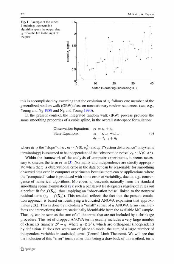
We highlight here the key features of Young’s recursive algorithms of SDR byconsidering the case of p = 1 and z(X) = g(X) + e, with e ∼ N(0, σ 2); i.e., werewrite the smoothing problem as zk = sk + ek , where k = 1, . . . ,N and sk is theestimate of g(Xk). To make the recursive approach meaningful, the MC sample needsto be sorted in ascending order with respect to X: i.e., k and k − 1 subscripts areadjacent elements under such ordering (see Fig. 1), implying 0 ≤ X1 < X2 < · · · <
Xk < · · · < XN ≤ 1.To recursively estimate the sk in SDR, it is necessary to characterize it in some
stochastic manner, borrowing from nonstationary time series processes. In general
370 M. Ratto, A. Pagano
Fig. 1 Example of the sortedk-ordering: the recursivealgorithm spans the output datazk from the left to the right ofthe plot
this is accomplished by assuming that the evolution of sk follows one member of thegeneralized random walk (GRW) class on nonstationary random sequences (see, e.g.,Young and Ng 1989 and Ng and Young 1990).
In the present context, the integrated random walk (IRW) process provides thesame smoothing properties of a cubic spline, in the overall state-space formulation:
Observation Equation: zk = sk + ek
State Equations: sk = sk−1 + dk−1dk = dk−1 + ηk
(3)
where dk is the “slope” of sk , ηk ∼ N(0, σ 2η ) and ηk (“system disturbance” in systems
terminology) is assumed to be independent of the “observation noise” ek ∼ N(0, σ 2).Within the framework of the analysis of computer experiments, it seems neces-
sary to discuss the term ek in (3). Normality and independence are strictly appropri-ate when there is observational error in the data but can be reasonable for smoothingobserved data even in computer experiments because there can be applications wherethe “computed” value is produced with some error or variability, due to, e.g., conver-gence of numerical algorithms. Moreover, ek descends naturally from the standardsmoothing spline formulation (2): such a penalized least-squares regression rules outa perfect fit for f (Xk), thus implying an “observation noise” linked to the nonzeroresidual term (zk − f (Xk)). This residual reflects the fact that the present emula-tion approach is based on identifying a truncated ANOVA expansion that approxi-mates z(X). This is done by including a “small” subset of q ANOVA terms (main ef-fects and interactions) that are statistically identifiable from the available MC sample.Thus, ek can be seen as the sum of all the terms that are not included by a shrinkageprocedure. This set of dropped ANOVA terms usually includes a very large numberof elements (namely 2p − q , where q � 2p), which are orthogonal (independent)by definition. It does not seem out of place to model the sum of a large number ofindependent variables in statistical terms (Central Limit Theorem). We will see thatthe inclusion of this “error” term, rather than being a drawback of this method, turns
Recursive algorithms for smoothing spline ANOVA models 371
out to be an advantage (see the examples in Sect. 3), since it implies that emulation(and therefore “prediction” at untried X values) is performed only using statisticallysignificant ANOVA terms, enhancing the robustness of out-of-sample performances.
Given the ascending ordering of the MC sample, sk can be estimated by using therecursive Kalman filter (KF) and the associated recursive fixed interval smoothing(FIS) algorithm (see, e.g., Kalman 1960; Young 1999 for details).
First, it is necessary to optimize the hyper-parameters associated with the state-space model (3), namely the white noise variances σ 2 and σ 2
η . In fact, by a simplereformulation of the KF and FIS algorithms, the IRW model can be entirely charac-terized by one noise variance ratio (NVR) hyper-parameter, where NVR = σ 2
η /σ 2.This NVR value is, of course, unknown a priori and needs to be optimized: for ex-ample, in the above references, this is accomplished by maximum likelihood (ML)optimization using prediction error decomposition (Schweppe 1965). The NVR playsthe inverse role of a smoothing parameter: the smaller the NVR, the smoother the es-timate of sk (and at the limit NVR = 0, sk will be a straight line). Given the NVR,the FIS algorithm then yields an estimate sk|N of sk at each data sample, and it canbe seen that the sk|N from the IRW process is the equivalent of f (Xk) in the cubicsmoothing spline model. At the same time, the recursive procedures provide, in anatural way, standard errors of the estimated sk|N that allow for the testing of theirrelative significance.
We need to clarify here the meaning of the ML optimization in this recursivecontext. We first observe that, to avoid a perfect fit solution, a penalty term is usedin the “classical” smoothing spline estimates. The “penalty” appears in the objectivefunction (GCV, GML, etc.) which is used to optimize the λ’s. In this way one maylimit the “degrees of freedom” of the spline model.
For example, in GCV, we have to find a λ that minimizes
GCVλ = 1/N ·∑
k(zk − fλ(Xk))2
(1 − df (λ)/N)2, (4)
where df ∈ [0,N ] denotes the “degrees of freedom” as a function of λ. Similarly, inthe SDR notation, we look for an NVR minimizing
GCVNVR = 1/N ·∑
k(zk − sk|N)2
(1 − df (NVR)/N)2, (5)
where the “degrees of freedom” df depend on the NVR (by the above-mentionedequivalence).
Remark 1 Without the penalty term, the optimum would always be attained at λ = 0(or NVR → ∞), i.e., perfect fit.
A perfect fit “optimal” solution would never happen within the SDR recursivecontext. In this case penalty is directly associated with the estimate procedure, bythe fact that the prediction error decomposition (ML) estimate is based on the filteredestimate sk|k−1 = sk−1 +dk−1 and not on the smoothed estimate sk|N . Namely, in ML
372 M. Ratto, A. Pagano
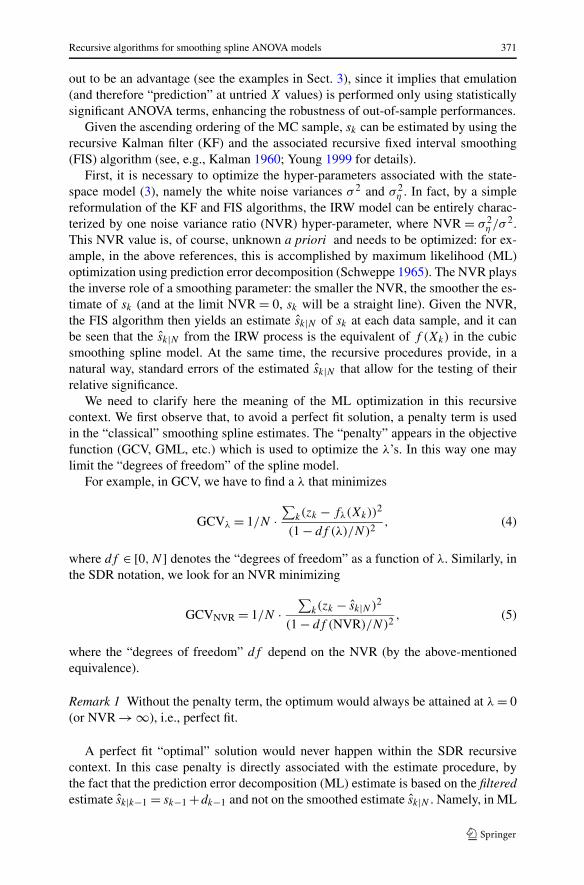
Fig. 2 Picture of the one stepahead predictions of the IRWprocess in the case ofNVR → ∞. The stars/dottedline denote the zk data series,while the squares denote the onestep ahead prediction sk|k−1
estimation, we find the NVR that maximizes the log-likelihood function L, where:
−2 · log(L) = const +N∑
k=3
log(1 + Pk|k−1) + (N − 2) · log(σ 2
),
σ 2 = 1
N − 2
N∑
k=3
(zk − sk|k−1)2
(1 + Pk|k−1), (6)
where σ 2 is the “weighted average” of the squared innovations (i.e., the predictionerror of the IRW model), and Pk|k−1 is the one step ahead forecast error of the statesk|k−1 provided by the KF (both Pk|k−1 and sk|k−1 are functions of NVR). Sincesk|k−1 is based only on the information contained in the sample values [1, . . . , k − 1](while smoothed estimates use the entire information set [1, . . . ,N ]), it can be easilyseen that the limit NVR → ∞ (λ → 0) is no longer a “perfect fit” situation, since azero variance for ek implies sk|k−1 = sk−1 + dk−1 = zk−1 + dk−1; i.e., the one stepahead prediction of zk is given by the linear extrapolation of the adjacent value zk−1,thus implying a nonzero prediction error in this limit case.
This is further exemplified in Fig. 2: the squares in the plots denote the one stepahead prediction sk|k−1 and the arrows show the linear extrapolation mechanism ofthe IRW process when NVR → ∞. Such a prediction departs considerably not onlyfrom a “perfect fit” situation but also from a “decent fit,” implying that the ML esti-mate will automatically penalize this kind of situation and provide the “right” valuefor the NVR (see also Wecker and Ansley 1983 for a discussion of this ML estimatorin the smoothing spline context).
To complete the equivalence between the SDR and cubic spline formulations, weneed to link the NVR estimated by the ML procedure to the smoothing parameters λ.It can be easily verified that by setting λ = 1/(NVR · N4), and with evenly spacedXk values, the f (Xk) estimate in the cubic smoothing spline model equals the sk|Nestimate from the IRW process. The present results are also in line with the cited

Recursive algorithms for smoothing spline ANOVA models 373
work of Wecker and Ansley (1983), who assume, however, a different stochastic formfor sk , namely an ARIMA(0,2,2) process.
As mentioned in the Introduction, this is not the only possible equivalence be-tween recursive algorithms and polynomial splines. For example, one can verifythat assuming a random walk stochastic process for sk with some ML optimizedNVR(RW) is equivalent to estimating a linear spline with smoothing parameterλ = 1/(NVR(RW) · N2) (see also Wecker and Ansley 1983).
The most interesting aspect of the SDR approach is that it is not limited to theunivariate case, but can be effectively extended to the most relevant multivariate one.In the general additive case (1), for example, the recursive procedure needs to beapplied, in turn, for each term fj (Xj,k) = sj,k|N , requiring a different sorting strategyfor each sj,k|N . Hence, the “backfitting” procedure, as described in Young (2000) andYoung (2001), is exploited (see Appendix A.1). This procedure provides both MLestimates of all NVRj ’s and the smoothed estimates of the additive terms sj,k|N . Itcan be easily verified that the equivalence between the λ’s and NVRs presented forp = 1 also holds for the additive model with p > 1. So, the estimated NVRj ’s can beconverted into λj values using λj = 1/(NVRj · N4), allowing us to put the additivemodel into the standard cubic spline form.
2.2 ANOVA models with interaction functions
The additive model concept (1) can be generalized to include two-way (and higher)interaction functions via the functional ANOVA decomposition (Wahba 1990; Gu2002). For example, we can let
f (X) = f0 +p∑
j=1
fj (Xj ) +p∑
j<i
fj,i(Xj ,Xi). (7)
In the ANOVA smoothing spline context, corresponding optimization problemswith interaction functions and their solutions can be obtained conveniently with thereproducing kernel Hilbert space (RKHS) approach (see Wahba 1990). In the SDRcontext, we propose here to formalize an interaction function as the product of twostates s1 · s2, each of them characterized by an IRW stochastic process. Hence, theestimation of a single interaction term z∗(Xk) = f (X1,k,X2,k) + ek is expressed as
Observation Equation: z∗k = sI
1,k · sI2,k + ek
State Equations: (j = 1,2) sIj,k = sI
j,k−1 + dIj,k−1
dIj,k = dI
j,k−1 + ηIj,k
(8)
where z∗ is the model output after the main effects are taken out, I = 1,2 is the multi-index denoting the interaction term under estimation, and ηI
j,k ∼ N(0, σ 2ηIj
). The two
terms sIj,k are estimated iteratively by running the recursive procedure in turn; i.e.,
– take an initial estimate of sI1,k and sI
2,k by regressing z with the product of simple
linear or quadratic polynomials p1(X1) · p2(X2) and set sI,0j,k = pj (Xj,k);

374 M. Ratto, A. Pagano
– iterate i = 1,2:– fix s
I,i−12,k and estimate NV RI
1 and sI,i1,k using the recursive procedure;
– fix sI,i1,k and estimate NV RI
2 and sI,i2,k using the recursive procedure;
– the product sI,21,k ·sI,2
2,k obtained after the second iteration provides the recursive SDRestimate of the interaction function.
The latter stopping criterion is a convenient choice to limit the computation time,and is due to the observation that the estimate of the interaction term never changedtoo much in any subsequent iteration.
Unfortunately, in the case of interaction functions we cannot derive an explicitand full equivalence between SDR and cubic splines of the type mentioned for first-order ANOVA terms. Therefore, in order to be able to exploit the estimation resultsin the context of a smoothing spline ANOVA model, we propose to take a differentapproach, similar to the ACOSSO case.
2.3 Very short summary of ACOSSO
We make the usual assumption that f ∈ F , where F is an RKHS. The space F canbe written as an orthogonal decomposition F = {1} ⊕ {⊕q
j=1 Fj }, where each Fj isitself an RKHS and j = 1, . . . , q spans ANOVA terms of various orders. Typically, q
includes the main effects plus relevant interaction terms.We reformulate (2) for the general case with interactions using the function f that
minimizes
1
N
N∑
k=1
(zk − f (Xk)
)2 + λ0
q∑
j=1
1
θj
∥∥P jf∥∥2
F , (9)
where P jf is the orthogonal projection of f onto Fj and the q-dimensional vec-tor θj of smoothing parameters needs to be optimized somehow. This is typicallya formidable problem, and in the simplest case θj is set to one, with the single λ0
estimated by GCV or GML.Problem (9) also poses the issue of selection of Fj terms: this is tackled rather
effectively within the COSSO/ACOSSO framework.The COSSO (Lin and Zhang 2006) penalizes the sum of norms, using a Least
Absolute Shrinkage and Selection Operator (LASSO)-type penalty (Tibshirani 1996)for the ANOVA model, which allows us to identify the informative predictor termsFj with an estimate of f that minimizes
1
N
N∑
k=1
(zk − f (Xk)
)2 + λ
Q∑
j=1
∥∥P jf∥∥
F (10)
using a single smoothing parameter λ, and where Q includes all ANOVA terms to bepotentially included in f , e.g., with a truncation up to second- or third-order interac-tions.

Recursive algorithms for smoothing spline ANOVA models 375
It can be shown that the COSSO estimate is also the minimizer of
1
N
N∑
k=1
(zk − f (Xk)
)2 +Q∑
j=1
1
θj
∥∥P jf∥∥2
F (11)
subject to∑Q
j=1 1/θj < M (where there is a 1-1 mapping between M and λ). So wecan think of the COSSO penalty as the traditional smoothing spline penalty plus apenalty on the Q smoothing parameters used for each component. The LASSO-typepenalty has the effect of setting some of the functional components (Fj ’s) equal tozero (e.g., the variable Xj or the interaction (Xj ,Xi) is not in the model); thus, it“automatically” selects the appropriate subset q of terms out of the Q “candidates.”The key property of COSSO is that with one single smoothing parameter (λ or M)it provides proper estimates of all θj parameters: therefore, it considerably improvesproblem (9) with θj = 1 (still with one single smoothing parameter λ0) and is muchmore computationally efficient than the full problem (9) with optimized θj ’s.
In the adaptive COSSO (ACOSSO) of Storlie et al. (2011), f ∈ F minimizes
1
N
N∑
k=1
(zk − f (Xk)
)2 + λ
q∑
j=1
wj
∥∥P jf∥∥
F , (12)
where 0 < wj ≤ ∞ are weights that depend on an initial estimate of f , either us-ing (9) with θj = 1 or the COSSO estimate (10). The adaptive weights are ob-tained as wj = ‖P j f ‖−γ
L2, typically with γ = 2 and the L2 norm ‖P j f ‖L2 =
(∫
(P j f (X))2dX)1/2. The use of adaptive weights improves the predictive capabilityof ANOVA models with respect to the COSSO case.
2.4 Combining SDR and ACOSSO for interaction functions
There is an obvious way of exploiting the SDR identification and estimation steps inthe ACOSSO framework: namely, the SDR estimates of additive and interaction func-tion terms can be taken as the initial f used to compute the weights in the ACOSSO.However, this would be a minimal approach, whereas the SDR identification andestimation provides more detailed information about fj terms that is worth exploit-ing. We define K〈j〉 to be the reproducing kernel (r.k.) of an additive term Fj of theANOVA decomposition of the space F . In the cubic spline case, this is constructed asthe sum of two terms K〈j〉 = K01〈j〉 ⊕ K1〈j〉, where K01〈j〉 is the r.k. of the parametric(linear) part and K1〈j〉 is the r.k. of the purely nonparametric part. The second-orderinteraction terms are constructed as the tensor product of the first-order terms, for atotal of four elements, i.e.,
K〈i,j〉 = (K01〈i〉 ⊕ K1〈i〉) ⊗ (K01〈j〉 ⊕ K1〈j〉)
= (K01〈i〉 ⊗ K01〈j〉) ⊕ (K01〈i〉 ⊗ K1〈j〉) ⊕ (K1〈i〉 ⊗ K01〈j〉) ⊕ (K1〈i〉 ⊗ K1〈j〉).(13)
376 M. Ratto, A. Pagano
In general, considering problem (9), one should attribute a specific coefficient θ〈·〉to each single element of the r.k. of Fj (see, e.g., Gu 2002, Chap. 3), i.e. two θ ’sfor each main effect, four θ ’s for each two-way interaction, and so on. In fact, eachFj would be optimally fitted by opportunely choosing weights in the sum of K〈·,·〉elements. This, however, makes the estimation problem rather complex, so, usually,the tensor product (13) is directly used, without tuning the weights of each elementof the sum. This strategy is also applied in ACOSSO.
Instead, we propose to use SDR estimates of interaction to set the weights.In particular, we can see that the SDR estimate of the interaction (8) is given by the
product of two univariate cubic splines. So, one can easily decompose each estimatedsIj into the sum of a linear (sI
01〈j〉) and nonparametric term (sI1〈j〉). This provides a
decomposition of the SDR interaction of the form
sIi · sI
j = sI01〈i〉sI
01〈j〉 + sI01〈i〉sI
1〈j〉 + sI1〈i〉sI
01〈j〉 + sI1〈i〉sI
1〈j〉, (14)
which can be thought of as a proxy of the four elements of the r.k. of the second-ordertensor product cubic spline.
This suggests that a natural use of the SDR identification and estimation in theACOSSO framework is to apply specific weights to each element of the r.k. K〈·,·〉 in(13). In particular, the weights are the L2 norms of each of the four elements esti-mated in (14). We will show in the examples that this choice leads to significant im-provement in the accuracy of ANOVA models with respect to the original ACOSSOapproach.
2.5 Kriging method: the DACE Matlab toolbox
DACE (Lophaven et al. 2002) is a Matlab toolbox used to construct kriging approx-imation models on the basis of data from computer experiments. Once we have thisapproximate model, we can use it as a surrogate model (emulator, meta-model).
We briefly highlight the main features of DACE.Keeping wherever possible the same notation that we used previously, the kriging
model can be expressed as a regression
z(X) = β1f1(X) + · · · + βqfq(X) + ζ(X), (15)
where fi, i = 1, . . . , q are deterministic regression terms, βi are the related regressioncoefficients, and ζ is a zero-mean random process whose variance depends on theprocess variance ω2 and on the correlation R(v,w) between ζ(v) and ζ(w). Thetoolbox provides a set of correlation functions defined as
R(θ, v,w) =∏
j=1:pRj (θj ,wj − vj ).
In particular, for the generalized exponential correlation function, used in the nextsection, one has
Rj (θj ,wj − vj ) = exp(−θj |wj − vj |θp+1
).
Recursive algorithms for smoothing spline ANOVA models 377
Then, we can define R as the correlation matrix at the design points (i.e., Ri,j =R(θ,Xi , Xj )) and the matrix r(X) = [R(X1,X), . . . , R(XN,X)], X being an untriedpoint. Similarly, we define f = [f1(X) · · ·fq(X)]′ and F = [f (X1) · · ·f (XN)]′; i.e.,F stacks in matrix form all values of f at the design points. Then, the regressionproblem Fβ ≈ Z has a GLS solution given by
β∗ = (F ′R−1F
)−1F ′R−1Z,
which gives the predictor at untried X
z(X) = f (X)′β∗ + r(X)′γ ∗,
where γ ∗ is computed as γ ∗ = R−1(Z − Fβ∗).Of course, the proper estimation of the kriging emulator requires one to optimize
the hyper-parameters θ in the correlation function: this is typically performed bymaximum likelihood.
It is easy to check that the kriging predictor interpolates Xj , if the latter is a designpoint. As far as regression models are concerned, the choice for f can be chosen fromthe following options:
Constant q = 1, f1 = 1Linear q = p + 1, f1 = 1, f2 = X1, . . . , fp+1 = Xp
Quadratic q = 12 (p + 1)(p + 2), f1 = 1, f2 = X1, . . . , fp+1 = Xp, fp+2 = X2
1,
fp+3 = X1X2 . . .
It seems useful to underline that one major difference between DACE and ANOVAsmoothing is the absence of any “observation error” in (15). This is a natural choicewhen analyzing computer experiments, and it aims to exploit the “zero-uncertainty”feature of this kind of data. This, in principle, makes the estimation of kriging emula-tors very efficient, as confirmed by the many successful applications described in theliterature, and justifies the great success of this kind of emulator among practitioners.It also seems interesting to mention the “nugget” effect, which is also used in thekriging literature (see Wagner 2010 for an application of this in the present issue).This is nothing other than a “small” error term in (15), and it often reduces some nu-merical problems encountered in the estimation of the kriging emulator to the formof (15). The addition of a nugget term leads to kriging emulators that smooth, ratherthan interpolate, making them more similar to ANOVA models.
3 Examples
Storlie et al. (2008) performed an extensive analysis and comparison of meta-modeling approaches for the estimation of total sensitivity indices. Their main con-clusions were:
– simple models like quadratic regressions and additive smoothing splines can workvery well, especially for small sample sizes;
– for larger sample sizes, more flexible approaches (MARS, ACOSSO, MLE GP inparticular) can provide better estimations;

378 M. Ratto, A. Pagano
– GP does not outperform smoothing methods in estimating sensitivity indices.
The present paper does not substantially modify these results on sensitivity indicesestimation, so we concentrate here on the forecast performance (out-of-sample R2 )of the different methods in predicting the function values at untried X’s.
We compared the combined SDR-ACOSSO approach with ACOSSO and DACEon several examples (full details including Matlab routines are freely available onrequest):
• we checked the behavior of the SDR procedure proposed in Sect. 2.2 in identifyingsingle two-way interaction functions;
• we performed full emulation exercises, considering multivariate analytic functions.
Concerning DACE, we always use the generalized exponential correlation func-tion to estimate the emulator. Moreover, we include the nugget term in the singlesurface identification of Sect. 3.1, while the standard interpolating form of DACE isconsidered in the full emulation exercises of Sect. 3.2.
3.1 Single surface identification
First we checked the behavior of SDR in identifying single two-way interaction func-tions; i.e., we considered a number of surfaces z(X1,X2) = g(X1,X2) + e, withe ∼ N(0, σ 2), using different levels of signal-to-noise ratios SNR = V (z)/V (e): verylarge (SNR > 10), medium (SNR ∼ 3), very small (SNR ∼ 0.1).
This kind of exercise is useful since it mimics the typical situation of the “back-fitting” procedure adopted in the SDR method: in such a procedure each term ofthe ANOVA decomposition is identified and analyzed in turn, with the rest of theANOVA terms acting as a sort of “noise.” So g(X1,X2) can be seen here as rep-resenting one single interaction term, to be identified among a number of ANOVAterms, represented by e. So, very large SNR represents the case of a predominantinteraction term in the ANOVA model, and vice versa for very small SNR. We com-pared SDR results with standard GCV estimation and with DACE (extended to in-clude observation noise/nugget) using a training MC sample X of 256 elements andtested the out-of sample performance of each method in predicting the “noise-free”signal g(X1,X2) using a new validation sample X∗ of dimension 256. We repeatedthis exercise on 100 random replicas for each function and each SNR.
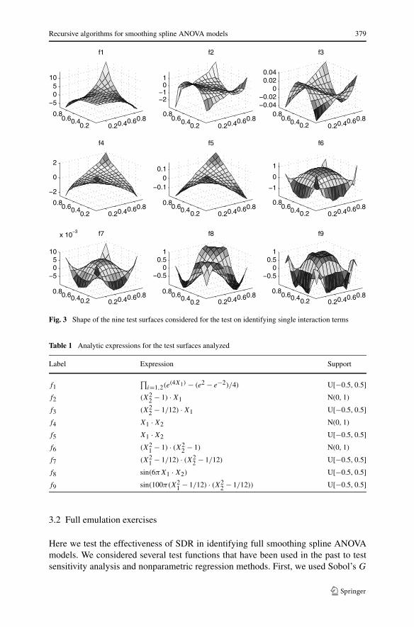
We considered nine types of surfaces of increasing order of complexity (i.e., 27different surface identifications, each replicated 100 times). The shapes of the sur-faces are shown in Fig. 3, while their analytic expressions are shown in Table 1.
In Fig. 4 we can see that for only one out of the nine surfaces (f9), DACE out-performed SDR or GCV estimation. This is probably to be expected since this isa pure smoothing problem, obviously more tailored for smoothing methods. In theother cases, SDR and GCV gave similar results, when the four terms in (14) havesimilar weights, while SDR was more efficient in identifying surfaces, where linearand nonparametric parts need to be better differentiated (f6, f7, f9). These resultsdemonstrate that the SDR identification step described in Sect. 2.2 is effective foridentifying interaction functions.
Recursive algorithms for smoothing spline ANOVA models 379
Fig. 3 Shape of the nine test surfaces considered for the test on identifying single interaction terms
Table 1 Analytic expressions for the test surfaces analyzed
Label Expression Support
f1∏
i=1,2(e(4X1) − (e2 − e−2)/4) U[−0.5, 0.5]
f2 (X22 − 1) · X1 N(0, 1)
f3 (X22 − 1/12) · X1 U[−0.5, 0.5]
f4 X1 · X2 N(0, 1)
f5 X1 · X2 U[−0.5, 0.5]
f6 (X21 − 1) · (X2
2 − 1) N(0, 1)
f7 (X21 − 1/12) · (X2
2 − 1/12) U[−0.5, 0.5]
f8 sin(6πX1 · X2) U[−0.5, 0.5]
f9 sin(100π(X21 − 1/12) · (X2
2 − 1/12)) U[−0.5, 0.5]
3.2 Full emulation exercises
Here we test the effectiveness of SDR in identifying full smoothing spline ANOVAmodels. We considered several test functions that have been used in the past to testsensitivity analysis and nonparametric regression methods. First, we used Sobol’s G

380 M. Ratto, A. Pagano
Fig. 4 Out-of-sample R2 for the nine test surfaces of the three methods applied: SDR, ACOSSO, DACE
function (Archer et al. 1997), which can be used to generate test cases over a widespectrum of difficulty and dimensionality p. It is defined as
G = G(X1,X2, . . . ,Xp, a1, a2, . . . , ap)
=p∏
i=1
|4Xi − 2| + ai
1 + ai
. (16)
The characteristics of the G-functions are driven both by the dimension (p) andby the spectrum of the coefficients ai . Low values of ai , such as ai = 0, imply animportant first-order effect. If more than one factor has low ai ’s, then high interac-tion effects will also be present. The worst case for this function is where all ai ’sare zero; i.e., all factors are equally important and all factors interact. If only a cou-ple of ai ’s are zero and all the others are large (e.g., ai ≥ 9), then we have a rela-tively easy test case, with just two important factors and a single two-way interactionterm.
We considered the following four cases for the G-function, characterized by anincreasing difficulty, due to the dimensionality of the problem (increasing p) or thedegree of interactions (spectrum of ai coefficients):
– p = 4, a = [0,1,5,99], labeled as “simple” in Table 2;– p = 4, a = [0,0.01,0.2,0.5], labeled as “nasty” in Table 2;– p = 8, a = [0,1,4.5,9,99,99,99,99], labeled as “simple” in Table 2;– p = 10, a = [0,0.1,0.2,0.3,0.4,0.5,0.6,0.7,0.8,0.9], labeled as “nasty” in Ta-
ble 2.

Recursive algorithms for smoothing spline ANOVA models 381
We also use here a modified G-function, defined as
G∗ = G∗ (X1,X2, . . . ,Xp, a1, a2, . . . , ap, δ1, δ2, . . . , δp,α1, α2, . . . , αp
)
=p∏
i=1
(1 + αi) · |2(Xi + δi − [Xi + δi]) − 1|αi + ai
1 + ai
, (17)
where δi ∈ [0,1], αi > 0 are shift and curvature parameters, respectively, and [Xi +δi] is the integer part of Xi + δi . If αi = 1 and δi = 0, G∗ degenerates to the G-function.
For this modified G∗-function, we analyzed the same cases listed previously forthe standard G-function, but using αi = 0.25 and δi = 0. These are essentially modi-fied versions of the G-function examples, where we add more curvature in the model.
We also analyzed two test functions used in Storlie et al. (2011). In the first testfunction from Storlie et al. (2011), we have X uniform in [0,1]10 and the underlyingfunction is nonadditive:
f4(X) = g1(X1) + g2(X2) + g3(X3) + g4(X4) + g3(X1X2)
+ g2((X1 + X3)/2
) + g1(X3X4) (18)
and, therefore X5, . . . ,X10 are uninformative (dummy) variables.In the second test function from Storlie et al. (2011), we have X uniform in [0,1]12
and the underlying regression function is additive:
f12(X) = g1(X1) + g2(X2) + g3(X3) + g4(X4)
+ 1.5 · g1(X5) + 1.5 · g2(X6) + 1.5 · g3(X7) + g4(X8)
+ 2 · g1(X9) + 2 · g2(X10) + 2 · g3(X11) + 2 · g4(X12). (19)
The following four functions on [0, 1] are used as building blocks in (18) and (19):
g1(t) = t; g2(t) = (2t − 1)2; g3(t) = sin(2πt)
2 − sin(2πt);
g4(t) = 0.1 sin(2πt) + 0.2 cos(2πt) + 0.3 sin2(2πt) + 0.4 cos3(2πt)
+ 0.5 sin3(2πt).
(20)
We considered training samples of growing dimension 64, 128, and 256 to es-timate the emulators and used a new validation sample of the same dimension tocheck the out-of-sample performance. We repeated the analysis 100 times for eachfunction and each method. We show detailed box-plots of the out-of-sample R2 inFigs. 5 through 7, while Table 2 synthesizes the out-of-sample performance of thethree methods, with stars highlighting the best performing method.
Considering small sample sizes (N = 64, Fig. 5), there is one test function(namely G∗, p = 10, “nasty”) which is very difficult to predict. For that function,the only method which is able to give an out-of-sample fit is SDR-ACOSSO, whileACOSSO and especially DACE are not capable of providing any reasonable fit. For

382 M. Ratto, A. Pagano
Fig. 5 Box-plots of the out-of-sample R2 for the test models in Table 2, applying SDR, ACOSSO, DACE.Sample size is N = 64
all other test functions, both SDR-ACOSSO and DACE behave well, if the median ofthe R2 distribution is only considered. However, for six of these test functions, the R2
distribution of DACE presents “outliers” with very bad fit. This implies that, althoughthe median of the R2’s is generally somewhat better for DACE, SDR-ACOSSO es-timations are more robust and stable since bad outliers never occur. ACOSSO some-times competes with SDR, in some other cases it performs a bit worse, but in onecase (G∗, p = 8, “simple”) it is clearly worse. Overall, we can say that, due to theoccurrence of bad “outliers” for DACE, the SDR-ACOSSO seems overall the bestmethod for small sample sizes.
Considering N = 128 in Fig. 6, we can see that DACE R2 is affected by bad out-liers for two test functions, making SDR preferable in terms of robustness, althoughin terms of median DACE is often better. ACOSSO almost always lags behind theother two methods. Two results are worth noting: (i) when DACE has the best per-formance, we can see that the SDR identification step is able to fill a large part ofthe gap between ACOSSO and DACE; (ii) for the additive f12 test function, SDRoutperforms the other two methods (we recall that for additive models, SDR is notcombined with ACOSSO, but directly provides the smoothing spline ANOVA modelfrom the ML estimated NVRs).
Recursive algorithms for smoothing spline ANOVA models 383
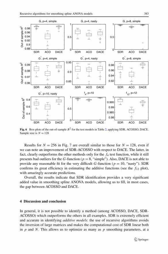
Fig. 6 Box-plots of the out-of-sample R2 for the test models in Table 2, applying SDR, ACOSSO, DACE.Sample size is N = 128
Results for N = 256 in Fig. 7 are overall similar to those for N = 128, even ifwe can note an improvement of SDR-ACOSSO with respect to DACE. The latter, infact, clearly outperforms the other methods only for the f4 test function, while it stillpresents bad outliers for the G-function (p = 8, “simple”). Also, DACE is not able toprovide any reasonable fit for the very difficult G-function (p = 10, “nasty”). SDRconfirms its great efficiency in estimating the additive functions (see the f12 plot),with amazingly accurate predictions.
Overall, the results indicate that SDR identification provides a very significantadded value in smoothing spline ANOVA models, allowing us to fill, in most cases,the gap between ACOSSO and DACE.
4 Discussion and conclusion
In general, it is not possible to identify a method (among ACOSSO, DACE, SDR-ACOSSO) which outperforms the others in all examples. SDR is extremely efficientand accurate in identifying additive models: the use of recursive algorithms avoidsthe inversion of large matrices and makes the computational cost of SDR linear bothin p and N . This allows us to optimize as many as p smoothing parameters, at a

384 M. Ratto, A. Pagano
Fig. 7 Box-plots of the out-of-sample R2 for the test models in Table 2, applying SDR, ACOSSO, DACE.Sample size is N = 256
similar cost of, e.g., ACOSSO in which one single smoothing parameter M is opti-mized. The computational cost of ACOSSO and DACE increases nonlinearly with p
and N .In the case of ANOVA models with interaction components, ACOSSO confirms
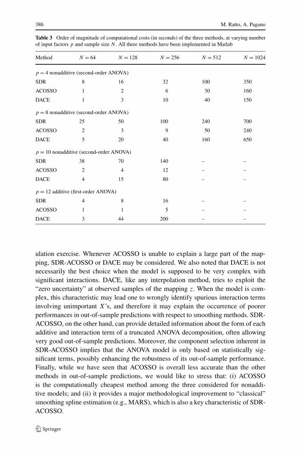
entirely its good performances in terms of efficiency and low computational cost.When the model includes interactions, SDR combined with ACOSSO improvesACOSSO in many cases, although at the price of a higher computational cost. Thisis due to the SDR estimation of each single ANOVA term in the backfitting loop,prior to the final ACOSSO optimization of M . So, while for additive models the ad-vantage of SDR is both low computational cost and accuracy, when interactions areincluded, the greater accuracy of SDR-ACOSSO has a cost, which does not exceeda few minutes in any cases (see Table 3). SDR-ACOSSO also compares very favor-ably with respect to DACE in many cases, even if there are cases where DACE out-performs SDR-ACOSSO in out-of-sample prediction. The main drawback of DACEseems to be the occurrence of very bad outliers in the distributions of R2, imply-ing some lack of robustness. The computational cost of DACE can be very sensi-tive to the underlying model. For each fixed dimension p and sample size N itsvariability can be of one order of magnitude (see Table 3). In terms of computa-tional burden, we suggest that SDR (for additive models) and ACOSSO (for modelswith interactions) should be taken as the first choice for a rapid and reliable em-

Recursive algorithms for smoothing spline ANOVA models 385
Table 2 SDR-ACOSSO, ACOSSO, and DACE: average R2 (out of sample) computed on 100 replicasfor different types of test functions. Stars indicate the method with best out-of-sample performance
Model Sample size SDR-ACOSSO ACOSSO DACE
G, p = 4 simple 64 0.9187 0.8960 0.5468
(0.9543a)
G, p = 4 simple 128 0.9881∗ 0.9392 0.9884∗G, p = 4 simple 256 0.9973∗ 0.9926 0.9973∗
G, p = 4 nasty 64 0.5104 0.5159∗ −0.5721
(0.3942a)
G, p = 4 nasty 128 0.6960∗ 0.5833 0.6008
G, p = 4 nasty 256 0.9105∗ 0.8507 0.8609
G, p = 8 simple 64 0.8603∗ 0.6906 −0.7945
(0.8367a) (0.9297a)
G, p = 8 simple 128 0.9679∗ 0.9008 0.9298
(0.9736a)
G, p = 8 simple 256 0.9924∗ 0.9164 0.9832
G, p = 10 nasty 256 0.1922∗ 0.1963∗ −0.0247
G∗, p = 4 simple 64 0.9613 0.9476 0.9701∗G∗, p = 4 simple 128 0.9831∗ 0.9759 0.9864∗G∗, p = 4 simple 256 0.9928∗ 0.9892 0.9940∗
G∗, p = 4 nasty 64 0.8556∗ 0.8460 0.7354
(0.8804a)
G∗, p = 4 nasty 128 0.9142∗ 0.9103 0.9162∗G∗, p = 4 nasty 256 0.9574∗ 0.9299 0.9534∗
G∗, p = 8 simple 64 0.9213 0.4393 0.9586∗G∗, p = 8 simple 128 0.9689 0.9435 0.9813∗G∗, p = 8 simple 256 0.9876 0.9736 0.9910∗
G∗, p = 10 nasty 64 0.2601∗ 0.0637 −21.4
(−0.0516a)
G∗, p = 10 nasty 128 0.6823 0.5845 0.7601∗G∗, p = 10 nasty 256 0.8166∗ 0.8061 0.8205∗
f4, p = 10 64 0.7621∗ 0.4815 −6.763
(0.5859a) (0.8303a)
f4, p = 10 128 0.9241 0.8819 0.971∗f4, p = 10 256 0.9806 0.9764 0.9927∗
f12, p = 12 64 0.8506 0.8276 0.8799∗(0.8809a) (0.8406a) (0.9205a)
f12, p = 12 128 0.9966∗ 0.9859 0.9947∗f12, p = 12 256 0.9999∗ 0.9996∗ 0.9996∗
aWe include the median of the R2 sample here, due to the presence of “outliers” with very bad fit (seeFigs. 5–7)
386 M. Ratto, A. Pagano
Table 3 Order of magnitude of computational costs (in seconds) of the three methods, at varying numberof input factors p and sample size N . All three methods have been implemented in Matlab
Method N = 64 N = 128 N = 256 N = 512 N = 1024
p = 4 nonadditive (second-order ANOVA)
SDR 8 16 32 100 350
ACOSSO 1 2 6 30 160
DACE 1 3 10 40 150
p = 8 nonadditive (second-order ANOVA)
SDR 25 50 100 240 700
ACOSSO 2 3 9 50 240
DACE 5 20 40 160 650
p = 10 nonadditive (second-order ANOVA)
SDR 38 70 140 – –
ACOSSO 2 4 12 – –
DACE 4 15 80 – –
p = 12 additive (first-order ANOVA)
SDR 4 8 16 – –
ACOSSO 1 1 5 – –
DACE 3 44 200 – –
ulation exercise. Whenever ACOSSO is unable to explain a large part of the map-ping, SDR-ACOSSO or DACE may be considered. We also noted that DACE is notnecessarily the best choice when the model is supposed to be very complex withsignificant interactions. DACE, like any interpolation method, tries to exploit the“zero uncertainty” at observed samples of the mapping z. When the model is com-plex, this characteristic may lead one to wrongly identify spurious interaction termsinvolving unimportant X’s, and therefore it may explain the occurrence of poorerperformances in out-of-sample predictions with respect to smoothing methods. SDR-ACOSSO, on the other hand, can provide detailed information about the form of eachadditive and interaction term of a truncated ANOVA decomposition, often allowingvery good out-of-sample predictions. Moreover, the component selection inherent inSDR-ACOSSO implies that the ANOVA model is only based on statistically sig-nificant terms, possibly enhancing the robustness of its out-of-sample performance.Finally, while we have seen that ACOSSO is overall less accurate than the othermethods in out-of-sample predictions, we would like to stress that: (i) ACOSSOis the computationally cheapest method among the three considered for nonaddi-tive models; and (ii) it provides a major methodological improvement to “classical”smoothing spline estimation (e.g., MARS), which is also a key characteristic of SDR-ACOSSO.

Recursive algorithms for smoothing spline ANOVA models 387
Appendix
A.1 The backfitting algorithm
We provide here a short summary of the backfitting algorithm, as described in Young(2000) and Young (2001). The basic reason why we need a backfitting procedure isto deal with the problems arising from the sorting strategy employed in the recursivealgorithms. Once we have a preliminary estimate of the state variables, we define a“modified dependent variable” series obtained by subtracting from zk all the otherterms on the right-hand side of (1).
The backfitting algorithm takes the following form:
1. start from an initial estimate of states s0i,k|N, i = 1, . . . , p, k = 1, . . . ,N ;
2. for backfitting iterations b = 1, . . . ,B
(a) for i = 1, . . . , p define the modified dependent variable zik = zk −∑
j �=i sb−1j,k|N ;
(b) estimate NVRi by the ML optimization;(c) get an updated estimate sb
i,k|N ;
(d) move to next b until no significant changes are detected in sbi,k|N .
3. the final NVRi ’s estimates are converted into the smoothing parameters λi ’s andthe estimated model is finally cast in the standard smoothing spline ANOVA form.
Remark 2 It is not necessary to update the NVRi estimates for all backfitting iter-ations b = 1, . . . ,B , but usually two backfitting iterations are sufficient for their ef-fective estimates. This significantly speeds up the computational cost of subsequentbackfitting iterations, that simply update, until convergence, sb
i,k|N . Usually B < 10.
Remark 3 Given the optimized NVRs, the backfitting algorithm provides estimatessBi,k|N that are equivalent to the smoothing spline estimate fi(Xi,k) obtained with
λi = 1/(NVRiN4).
References
Archer, G., Saltelli, A., Sobol’, I.: Sensitivity measures, ANOVA-like techniques and the use of bootstrap.J. Stat. Comput. Simul. 58, 99–120 (1997)
Gu, C.: Smoothing Spline ANOVA Models. Springer, Berlin (2002)Hodrick, T., Prescott, E.: Post-war US business cycles: an empirical investigation. Discussion paper n. 451,
Northwestern University, Evanston, IL (1981)Kalman, R.: A new approach to linear filtering and prediction problems. ASME Trans. J. Basic Eng. D 82,
35–45 (1960)Leser, C.: A simple method of trend construction. J. R. Stat. Soc. B 23, 91–107 (1961)Levy, S., Steinberg, D.: Computer experiments: A review. Adv. Stat. Anal. 94(4), 311–324 (2010)Lin, Y., Zhang, H.: Component selection and smoothing in smoothing spline analysis of variance models.
Ann. Stat. 34, 2272–2297 (2006)Lophaven, S., Nielsen, H., Sondergaard, J.: DACE A MATLAB kriging toolbox, Version 2.0. Technical Re-
port IMM-TR-2002-12, Informatics and Mathematical Modelling, Technical University of Denmark(2002). http://www.immm.dtu.dk/hbn/dace
Ng, C., Young, P.C.: Recursive estimation and forecasting of non-stationary time series. J. Forecast. 9,173–204 (1990)

388 M. Ratto, A. Pagano
Ratto, M., Pagano, A., Young, P.C.: State dependent parameter meta-modelling and sensitivity analysis.Comput. Phys. Commun. 177, 863–876 (2007)
Schweppe, F.: Evaluation of likelihood functions for Gaussian signals. IEEE Trans. Inf. Theory 11, 61–70(1965)
Storlie, C., Bondell, H., Reich, B., Zhang, H.: Surface estimation, variable selection, and the nonparametricoracle property. Stat. Sin. (2011, in press). http://www3.stat.sinica.edu.tw/statistica/, preprint articleSS-08-241
Storlie, C.B., Swiler, L., Helton, J.C., Sallaberry, C.: Implementation and evaluation of nonparametric re-gression procedures for sensitivity analysis of computationally demanding models. SANDIA ReportSAND2008-6570, Sandia Laboratories, Albuquerque, NM (2008)
Tibshirani, R.: Regression shrinkage and selection via the lasso. J. R. Stat. Soc. B 58(1), 267–288 (1996)Wagner, T., Bröcker, C., Saba, N., Biermann, D., Matzenmiller, A., Steinhoff, K., Model of a thermome-
chanically coupled forming process based on functional outputs from a finite element analysis andfrom experimental measurements. Adv. Stat. Anal. 94(4), 389–404 (2010)
Wahba, G.: Spline Models for Observational Data. CBMS-NSF Regional Conference Series in AppliedMathematics (1990)
Wecker, W.E., Ansley, C.F.: The signal extraction approach to non linear regression and spline smoothing.J. Am. Stat. Assoc. 78, 81–89 (1983)
Weinert, H., Byrd, R., Sidhu, G.: A stochastic framework for recursive computation of spline functions:Part II, smoothing splines. J. Optim. Theory Appl. 30, 255–268 (1980)
Young, P.C.: Nonstationary time series analysis and forecasting. Prog. Environ. Sci. 1, 3–48 (1999)Young, P.C.: Stochastic, dynamic modelling and signal processing: Time variable and state dependent
parameter estimation. In: Fitzgerald, W.J., Walden, A., Smith, R., Young, P.C. (eds.) Nonlinear andNonstationary Signal Processing, pp. 74–114. Cambridge University Press, Cambridge (2000)
Young, P.C.: The identification and estimation of nonlinear stochastic systems. In: Mees, AIea (ed.) Non-linear Dynamics and Statistics. Birkhäuser, Boston (2001)
Young, P.C., Ng, C.N.: Variance intervention. J. Forecast. 8, 399–416 (1989)Young, P.C., Pedregal, D.J.: Recursive and en-bloc approaches to signal extraction. J. Appl. Stat. 26, 103–
128 (1999)