using or hiding private information? an experimental study

HAL Id: halshs-00565157https://halshs.archives-ouvertes.fr/halshs-00565157

Submitted on 11 Feb 2011

HAL is a multi-disciplinary open accessarchive for the deposit and dissemination of sci-entific research documents, whether they are pub-lished or not. The documents may come fromteaching and research institutions in France orabroad, or from public or private research centers.

L’archive ouverte pluridisciplinaire HAL, estdestinée au dépôt et à la diffusion de documentsscientifiques de niveau recherche, publiés ou non,émanant des établissements d’enseignement et derecherche français ou étrangers, des laboratoirespublics ou privés.

Using or Hiding Private Information? An ExperimentalStudy of Zero-Sum Repeated Games with Incomplete

InformationNicolas Jacquemet, Frédéric Koessler

To cite this version:Nicolas Jacquemet, Frédéric Koessler. Using or Hiding Private Information? An Experimental Studyof Zero-Sum Repeated Games with Incomplete Information. 2011. �halshs-00565157�

https://halshs.archives-ouvertes.fr/halshs-00565157

https://hal.archives-ouvertes.fr

Documents de Travail du Centre d’Economie de la Sorbonne

Using or Hiding Private Information ?

An Experimental Study of Zero-Sum Repeated Games with

Incomplete Information

Nicolas JACQUEMET, Frédéric KOESSLER

2011.02

Maison des Sciences Économiques, 106-112 boulevard de L'Hôpital, 75647 Paris Cedex 13 http://centredeconomiesorbonne.univ-paris1.fr/bandeau-haut/documents-de-travail/

ISSN : 1955-611X

Using or Hiding Private Information?

An Experimental Study of Zero-Sum Repeated Games with

Incomplete Information ∗

Nicolas Jacquemet† Frederic Koessler‡

January 2011

∗We are very grateful to Kene Boun My for his assistance in designing the experiments and for his comments, aswell as to Marie Coleman, Marie-Laure Nauleau, Thibault Baron and Vincent Montamat for their research assistance.We thank Nick Feltovich for his comments and for sharing his data with us. We also thank Vincent Crawford, DavidEttinger, Francoise Forges, Guillaume Frechette, Jeanne Hagenbach, Philippe Jehiel, Rida Laraki, Paul Pezanis-Christou, Dinah Rosenberg, Larry Samuelson, Tristan Tomala, and Shmuel Zamir for comments and discussions onthe theory and/or on the experimental protocol. Financial support from an ACI grant by the French Ministry ofResearch is gratefully acknowledged.

†Paris School of Economics and University Paris I Pantheon–Sorbonne. Centre d’economie de la Sorbonne, 106Bd. de l’Hopital, 75013 Paris, France. [email protected].

‡Paris School of Economics – CNRS. 48, Boulevard Jourdan, 75014 Paris, France. [email protected].

1

Documents de Travail du Centre d'Economie de la Sorbonne - 2011.02

Abstract

This paper studies experimentally the value of private information in strictly competitive in-

teractions with asymmetric information. We implement in the laboratory three examples from

the class of zero-sum repeated games with incomplete information on one side and perfect

monitoring. The stage games share the same simple structure, but differ markedly on how

information should be optimally used once they are repeated. Despite the complexity of the

optimal strategies, the empirical value of information coincides with the theoretical prediction

in most instances. In particular, it is never negative, it decreases with the number of repetitions,

and it is nicely bounded below by the value of the infinitely repeated game and above by the

value of the one-shot game. Subjects are unable to completely ignore their information when it

is optimal to do so, but the use of information in the lab reacts qualitatively well to the type

and length of the game being played.

Keywords: Concavification; Laboratory experiments; Incomplete information; Value of infor-

mation; Zero-sum repeated games.

JEL Classification: C72; D82.

Resume

Cet article propose une analyse experimentale de la valeur de l’information privee dans des

interactions avec asymetrie d’information. Nous etudions dans le laboratoire trois exemples

tires de la classe des jeux a somme nulle repetes a information incomplete pour l’un des joueurs

et observation parfaite des actions. Les jeux partagent la meme structure simple, mais different

sur la facon dont l’information doit etre utilisee a l’optimum dans les version repetees. Malgre

la complexite des strategies optimales, la valeur empirique de l’information coincide avec la

prediction theorique dans la plupart des cas. En particulier, la valeur de l’information n’est

jamais negative, diminue avec le nombre de repetitions, et est minoree par la valeur du jeu

repete a l’infini et majoree par la valeur du jeu one-shot. Les sujets se revelent incapables

d’ignorer completement l’information quand il est optimal de le faire. Cependant, l’utilisation

de l’information reagit qualitativement dans la direction attendue au type et a la duree du jeu.

Mots-cles: Concavification; Experiences en laboratoire; Information incomplete; Valeur de

l’information; Jeux reptes a somme nulle.

2


Figure 1: Payoff matrices in the NR-games

Player 1

Player 2

Left Right

Top 10, 0 0, 10

Bottom 0, 10 0, 10

A1

Player 1

Player 2

Left Right

Top 0, 10 0, 10

Bottom 0, 10 10, 0

A2

1 Introduction

This paper studies experimentally the value of private information in strictly competitive interac-

tions with asymmetric information. We study three examples from the class of zero-sum repeated

games with incomplete information on one side and perfect monitoring, originating from Aumann

and Maschler (1966, 1967) and Stearns (1967). In this class of games, repetition is the channel

through which information is transmitted from one stage to another. Because of perfect monitoring,

information is (at least partially) revealed by the informed player’s action whenever he wants to

use it. Players’ preferences being diametrically opposed, the basic problem for the informed player

is to find out the optimal balance between using information as much as possible and revealing it

to his opponent as little as possible. On the other side, the uninformed player tries to find out the

actual information of his opponent and to make it the least valuable as possible.

As an illustration, Figure 1 presents the payoff matrices of one of the repeated game we imple-

ment in the laboratory. At the beginning of the repeated game, one of the two payoff matrices, A1

or A2, is drawn at random with the same probability. Player 1 (the row player) is privately informed

about the state of nature (matrix A1 or A2), and has a dominant action in each state: Top in A1,

Bottom in A2. This is clearly the best strategy for him in the one-shot game. Player 2 (the column

player) would like to play Right in A1 and Left in A2, but being uninformed he has to choose the

same action in both states, yielding an expected payoff equal to 5 for both players. Once the game

is repeated, the (perfectly observed) past decisions of the informed player become a signal about

the information of the row player: if his private information is fully used, then the column player

becomes aware of the actual state after the first stage, and plays his perfectly informed decision

forever: Right following Top (i.e., in A1) and Left following Bottom (i.e., in A2). In this case, the

payoff of the informed player is 0 in each further stage. Alternatively, the informed player can keep

his information private by using a strategy which is independent of the actual payoff matrix. The

cost of this non revealing strategy is to loose the rent derived from information in earlier stages.

How this trade-off is solved drives the extent to which information should be used or ignored by

the informed player.

3


The theory of zero-sum repeated games with incomplete information provides precise predictions

on players’ optimal strategies and the value (expected payoff) that each player can guarantee as

a function of the payoff matrices, the prior beliefs of the uninformed player and the number of

repetitions. One can tell when and at what rate the informed player should use (and thus reveal)

his information. From a behavioral point of view, zero-sum repeated games are one the most basic

context to study the revelation and value of information in strategic conflicts. Since equilibrium

strategies are equivalent to maxmin strategies, there is no equilibrium selection and coordination

problems between players. In addition, since payoffs are zero-sum, cooperation is not an issue and

social preferences should have limited effects on behavior even in repeated interactions between the

same players.

We investigate how the qualitative and quantitative features of the theory are satisfied in the

laboratory. We consider three types of repeated games, implemented as separate experimental

treatments. The games differ in that information should be either fully revealed (the FR-games),

partially revealed (the PR-games) or not revealed at all (the NR-games based on our introductory

example). To study the impact of the length of the game (i.e., the number of repetitions), each

of the three types of games is repeated from 1 to 5 stages. In order to allow subjects to get

some experience, each type of repeated game is repeated itself 20 times. To evaluate the value of

information we also consider two types of information structures in the NR-games: no information

(in which no player knows the actual payoff matrix) and incomplete information on one side (only

one player knows the payoff matrix).

Feltovich (1999, 2000) is to the best of our knowledge the only experimental analysis relying on

games from this class. Although the focus of his work is different from ours,1 his lab implementation

of a 2-stage zero-sum game (which corresponds to our introductory example based on the payoff

matrices of Figure 1) concludes that informed players use their information too much. This results in

an unexpectedly low average payoff for the informed subjects. This might yield the conjecture that

a curse of knowledge (Camerer, Loewenstein, and Weber, 1989; Loewenstein, Moore, and Weber,

2006) may occur in this class of games, in the sense that the actual value of information may become

negative when information is worth ignoring in longer repeated games. Indeed, the “naive” and

fully revealing strategy of the informed player – consisting in playing the stage-dominant action in

each stage of the repeated game – yields a zero payoff, while by playing non informatively – Top

and Bottom with the same probability whatever the state – the informed player’s expected payoff is

equal to 1/4. Hence, in longer repeated games subjects that are unable to ignore their information

may suffer severe losses compared to the situation where they would be uninformed.

This conjecture turns out to be false: we show that the empirical value of information is always

positive even in longer versions of the repeated games, and strictly positive when predicted so.

More generally, the empirical value of information coincides with the theoretical prediction in most

instances despite the complexity of the optimal strategies. We find strong support in favor of the

theoretical properties of the value of the games: in each type of repeated game the average empirical

payoff of the informed player is bounded above by the value of the one-shot game, is decreasing in

1It is aimed at comparing different models of learning (belief based learning vs. reinforcement learning).

4


the length of the game, and is bounded below by the value of the infinitely repeated game (also

known as “cav u”, the smallest concave function above the value of the game without information).

Nevertheless, in the most complex situations, the strategies supporting these results deviate from

the equilibrium strategies. Experimental subjects use private information with very high accuracy

when it’s worth using, but they are unable to correctly hide it when it is in their own interest to

do so. Observed behavior nonetheless reacts in the expected way to variations in the environment:

the flow of information from the informed to the uninformed player is higher the more valuable it

is for the informed player.

In Section 2 we present the basic model of zero-sum repeated games and some general and

important theoretical predictions. The three examples on which our experiment is based on and

more specific theoretical predictions for those games are provided in Section 3. Then, in Section 4

we present the experimental design implemented in the laboratory. In Section 5, we analyze players’

performances and behavior in the different experimental treatments, and we compare them with

theoretical benchmarks.

2 The theory of zero-sum repeated games

The theory of zero-sum repeated games with incomplete information started in the period 1966–

1968 and appeared in technical reports of the United States Arms Control and Disarmament Agency

(see Aumann and Maschler, 1966, 1967 and Stearns, 1967). This work is one of the fascinating

contribution for which Aumann was awarded the 2005 Nobel prize in economics. It was published

much later than the original reports in a book by Aumann and Maschler (1995). The most fun-

damental results and properties are surveyed in this book as well as in Mertens, Sorin, and Zamir

(1994), Sorin (2002) and Zamir (1992). The theory is at the origin of more recent analyses in non

zero-sum repeated games with incomplete information (Hart, 1985, Cripps and Thomas, 2003, Lovo

and Horner, 2009), repeated games with imperfect monitoring (Renault and Tomala, 2004, Obara,

2009), long cheap talk (Aumann and Hart, 2003, Krishna and Morgan, 2004, Goltsman, Horner,

Pavlov, and Squintani, 2009) and persuasion (Forges and Koessler, 2008, Kamenica and Gentzkow,

2009).

2.1 Model

In the simplest model of zero-sum repeated game, one of two finite zero-sum two-person payoff

matrices A1 or A2 is played repeatedly (the theory extends without further difficulty to any finite

number of possible states). The payoff matrix A1 (A2, respectively) is chosen once and for all ac-

cording to the common prior probability p1 = p ∈ [0, 1] (p2 = 1−p, respectively). When the matrix

is Ak, k ∈ {1, 2} is also called the type of player 1, or state. The real Ak(i, j) denotes player 1’s pay-

off when the state is k ∈ {1, 2}, player 1’s action is i ∈ I, and player 2’s action is j ∈ J . Player 2’s

payoff is a constant minus Ak(i, j), so player 2 is the minimizer and player 1 is the maximizer.

The value of the complete information game Ak is denoted by wk = maxx∈∆(I)miny∈∆(J) Ak(x, y)

(payoffs are extended to mixed actions in the usual way).

5


The n-stage repeated game with incomplete information is denoted Gn(p). Only player 1 knows

the state. That is, he knows from the beginning the payoff matrix, but player 2 does not. Both

players publicly observe past actions (perfect monitoring) but they do not observe their past payoffs

before the end of stage n (however, player 1 can obviously deduce his past payoffs from his knowledge

of the actual payoff matrix and past actions). Player 1’s average payoff is

1

n

n∑

m=1

Ak(im, jm),

when the state is k and the final history of play is ((i1, j1), (i2, j2), . . . , , (in, jn)). The value of

Gn(p) is denoted by vn(p).

2.2 Some general theoretical properties

We now present some of the general theoretical predictions in zero-sum repeated games. We

focus on those properties that help to find optimal strategies and expected payoffs, and/or that

are interesting to be tested experimentally. More precise statements can be found in the specific

surveys of the literature (e.g., Zamir, 1992).

One of the important property of the value function vn(p), which is useful for most mathematical

results in the literature, is its concavity in p, for all n. Since our experiment will held the probability

p constant across games (equal to 1/2), we are not able to check whether this property is satisfied in

the laboratory. We rather concentrate on how the repetition of the game affects the value, and use,

of information. Another very useful property is the following recursive formula, which considerably

helps to find the value of any (finitely) repeated game and the associated optimal strategies.

Proposition 1 (The recursive formula)

vn+1(p) =1

n+ 1max

x∈[∆(I)]2min

y∈∆(J)

(∑

k

pkAk(xk, y) + n∑

i∈I

(∑

k

pkxk(i))vn(p(x, i))

),

where p(x, i) =(

pkxk(i)∑kpkxk(i)

)k∈{1,2}

is the posterior probability over {1, 2} given action i and strategy

x of player 1.

Let u(p) be the value of the average game∑

k pkAk. The following proposition states the

positive value of information for player 1 whatever the length of the repeated game.2

Proposition 2 (Positive value of information) For all n and p, vn(p) ≥ u(p).

Albeit positive, the value of the repeated game is decreasing in the number of repetitions, as

stated in the following proposition. In particular, the value of the one-shot game, v1(p), is an

upper bound of the value of the repeated game whatever its length. The intuition is that when n

2This is obviously a general property of zero-sum games.

6


increases, the amount of information revealed by player 1 to player 2 is weakly increasing, so the

value for player 1 should decrease.

Proposition 3 (Decreasing value of information) For all p, vn(p) is weakly decreasing in n.

Interestingly, the value of the repeated game does not necessarily decrease up to the value of

the average game, even in the long run. The bound below vn(p) is in fact very easy to characterize

directly from the value of the average game, and is given by the concavification of u, denoted by

cav u, which is the smallest concave function which is higher than u. This extremely elegant result

is stated below.

Proposition 4 (Value in the long repeated games) limn→∞ vn(p) = cav u(p).

The theory of zero-sum repeated games with incomplete information provides lower bounds,

upper bounds, and comparative statics for the value of information as a function of the length and

payoff matrices of the repeated game. We now turn to the application of those results to instances

which lead to very different uses of information at equilibrium.

3 Analysis of the experimental games

Our experiment implements three modified examples from the literature in which information

should be fully revealed (the FR-games), should not be revealed (the NR-games), or should be

partially revealed (the PR-games) by the informed player. The examples have been designed in

order to ensure that each subject gets a positive payoff in all experiments, equilibrium payoffs are

similar across treatments, and there is a stage-dominant action for the informed player in every

state. All games are implemented as between-subjects treatments, with a common prior of p = 1/2

for each payoff matrix. We moreover consider 5 different lengths (n = 1, ..., 5), implemented as

within-subjects treatment variables.

3.1 Full revelation of information: the FR-games

Consider the payoff matrices presented in Figure 2. This is a modified (but not strategically

equivalent) version of the second example studied by Aumann and Maschler (1995). It has a

stage-dominant action, but contrary to the original example the informed player (player 1) cannot

guarantee the maximum payoff of the game, so the uninformed player (player 2) has an incentive

to use the information revealed by the informed player.

The values under complete information are w1 = w2 = 4. The stage-dominant (and fully

revealing) strategy Bottom (B) in A1 and Top (T ) in A2 is optimal in Gn(p) for all n and p. Hence,

player 2 plays any strategy in the first stage, and plays Right (R) after T and Left (L) after B.

This yields vn(p) =1n(5 + 4 + 4 + · · · ) = 1+4n

nfor all n and p, which tends to 4 when n tends to

infinity. On the contrary, by playing a non-revealing strategy, i.e., not using his private information

7


Figure 2: Payoff matrices in the FR-games

Player 1

Player 2

Left Right

Top 6, 4 4, 6

Bottom 0, 10 0, 10

A1

Player 1

Player 2

Left Right

Top 0, 10 0, 10

Bottom 4, 6 6, 4

A2

Figure 3: Concavification in the FR-game

p11/20

2.5

4

u

cav u

2/5 3/5

2.4

0

Note. Plot of the functions u(p) (dotted lines) and cav u(p) (plain lines) against p ∈ [0, 1]for the FR-games in Figure 2.

at all, player 1 would have get the value of the average game

pA1 + (1− p)A2 =

(6p 4p

4(1 − p) 6(1− p)

),

i.e.,

u(p) =

4(1− p) if p ≤ 2/5

10p(1− p) if p ∈ [2/5, 3/5]

4p if p ≥ 3/5,

which is always strictly smaller than 1+4nn

. Given the value of the average game, u(p), Figure 3 shows

the concavification in this game leads to a minimum value equal to v∞(p) = cav u(p) = 4 > u(p)

for all p ∈ (0, 1).

8


3.2 No revelation of information: the NR-games

Figure 1 in the Introduction presents payoff matrices which are strategically equivalent to those of

the first example in Aumann and Maschler (1995) and those studied experimentally by Feltovich

(1999, 2000). We consider two treatments. In the NR-NoInfo treatment, no player is informed

about the actual payoff matrix. This provides a control of the actual behavior of informed players.

In this version of the game, which is strategically equivalent to matching pennies, the value is

trivial: whatever the length n of the game, every player plays each action with probability one half,

leading to the average payoff u(1/2) = 2.5 for player 1. In the NR treatment, we implement the

same payoff matrices but with information asymmetries: player 1 is informed of the actual payoff

matrix, player 2 is not.

The values under complete information are w1 = w2 = 0, and in the one-shot incomplete

information game G1(1/2) the optimal strategy of player 1 is T in A1 and B in A2. Hence, v1(1/2) =

5 (any strategy of player 2 is optimal).3 Next, consider the n-stage incomplete information game. If

player 1 uses the previous stage-dominant strategy then player 2 learns the state in the second stage

and so would play R in A1 and L in A2. Hence, player 1’s average payoff would be 1n(5+0+0+· · · ) =

5n, which decreases to 0 when n increases. An alternative strategy for player 1 is to play a non

revealing strategy, which amounts to play the repeated average game

pA1 + (1− p)A2 =

(10p 0

0 10(1 − p)

),

whose value is u(p) = 10p(1 − p), so u(1/2) = 2.5 (player 1 plays each action with probability 1/2

independently of his information). This is clearly better than the previous fully revealing strategy

whenever n ≥ 2 since 2.5 ≥ 5/n for n ≥ 2. As shown in Figure 4, 2.5 is in fact the maximum payoff

that player 1 can guarantee in the long run because limn→∞ vn(1/2) = cav u(1/2) = u(1/2) = 2.5, so

the optimal strategy of player 1 in the infinitely repeated game consists in not using his information.

The value and optimal strategies of the finitely repeated games are much more difficult to

calculate. However, one can first notice that we necessarily have the simple property vn(1/2) ≥5(n+1)

2n for all n because player 1 is able to guarantee the average payoff 1n[(n− 1)52 + 5] by playing

a non revealing strategy during the first n− 1 stages, and the stage-dominant strategy in stage n.

But 5(n+1)2n is not exactly the value of Gn(1/2) for all n, it is only for n = 1, 2, 3 and n → ∞. For

4 ≤ n < ∞, player 1 should (very) partially reveal his information before the last stage of the

game, but his payoff is only very slightly above the lower bound of the value function.

One can compute the value vn(p) for all p ∈ [0, 1] and n ∈ {1, . . . , 5} using the recursive formula

of Proposition 1.4 Table 1 on page 12 represents these values for p = 1/2 and for n = 1, . . . , 5 . The

optimal strategy of player 1 depending on player 2’s posterior is deduced from the maxminimization

program of the recursive formula. Next, from the equilibrium conditions of player 1 (indifference

3More generally, v1(p) = 10(1− p) if p ≥ 1/2 and v1(p) = 10p if p ≤ 1/2.4The detailed calculations and explicit values of the function vn(·) are available from the authors upon request.

It is a stepwise continuous and linear function, and when n increases the number of intervals on which vn is definedrapidly increases.

9


Figure 4: Concavification in the NR-game

p11/20

2.5

0

cav u = u

Note. Plot of the functions u(p) (dotted lines) and cav u(p) (plain lines) against p ∈ [0, 1]for the NR-game in Figure 1.

when he uses a strictly positive mixed strategy) we deduce the equilibrium strategies of player 2.

This always yields a unique prediction for player 1. The optimal strategy of player 2 is not unique

in games G1(1/2), G2(1/2) and G5(1/2) in which a single free parameter remains (which can take

any value in a continuous interval). In all those situations we choose to select the strategy of

player 2 yielding a symmetric payoff for player 1 (the same expected payoff in A1 and A2). Of

course, since the games are zero-sum this selection has no impact on players’ ex-ante expected

payoffs and on player 1’s optimal strategy. Appendix A describes those optimal strategies and the

posterior beliefs of player 2 after every possible history of actions from player 1. Contrary to the

FR-games, Player 2’s strategies are very complex and are not markovian since they depend on the

history even for the same posterior beliefs.

With some abuse of language in the rest of the paper, and to make clear the distinction between

all treatments, we will sometime consider that the optimal strategy for the informed player in the

NR-games consists in not using his information, even if the exact optimal strategy is slightly

different for n ≥ 4.

3.3 Partial revelation of information: the PR-games

The game presented in Figure 5 is an intermediary case, which is strategically equivalent to the

third example in Zamir (1992), and somewhat simpler than the original example illustrating par-

tial revelation of information in Aumann and Maschler (1966, 1995). The values under complete

information are w1 = w2 = 3. In Gn(1/2), the fully revealing, stage-dominant strategy (T in A1,

B in A2) guarantees player 1 the average payoff 1n(6 + 3 + 3 + · · · ) = 3(1+n)

n, which decreases to 3

when n increases. On the other hand, by using a non revealing strategy player 1 can get the value

of the average game

pA1 + (1− p)A2 =

(3 + 6p 9− 6p 6p

3 + 6p 9− 6p 6− 6p

).

10


Figure 5: Payoff matrices in the PR-games

Player 1

Player 2

Left Center Right

Top 9, 0 3, 6 6, 3

Bottom 9, 0 3, 6 0, 9

A1

Player 1

Player 2

Left Center Right

Top 3, 6 9, 0 0, 9

Bottom 3, 6 9, 0 6, 3

A2

The optimal strategy of player 1 in the average game is T if p ≥ 1/2 and B if p ≤ 1/2. Hence,

player 2’s optimal strategy is

L if p ≤ 1/4,

R if 1/4 ≤ p ≤ 3/4,

C if p ≥ 3/4,

and the value is

u(p) =

3 + 6p if p ≤ 1/4,

6(1 − p) if 1/4 ≤ p ≤ 1/2,

6p if 1/2 ≤ p ≤ 3/4,

9− 6p if p ≥ 3/4.

Thus, when p = 1/2, player 1 can only guarantee 3 by using a non revealing strategy. Now, we

show that when p = 1/2 player 1 can guarantee at least 4.5 whatever n by using a partially revealing

(PR) strategy. If player 1 plays T forever with probability 3/4 and B forever with probability 1/4

in A1, and T forever with probability 1/4 and B forever with probability 3/4 in A2, then the

posteriors are

Pr(k = 1 | i = T ) = 3/4

Pr(k = 1 | i = B) = 1/4.

So, when he plays T , player 1’s conditional expected payoff is

3

4A1(T , ·) +

1

4A2(T , ·) =

3

4(9, 3, 6) +

1

4(3, 9, 0) = (7.5, 4.5, 4.5),

and when he plays B his conditional expected payoff is

1

4A1(B, ·) +

3

4A2(B, ·) =

1

4(9, 3, 0) +

3

4(3, 9, 6) = (4.5, 7.5, 4.5).

In both situations, whatever the strategy of player 2, the expected payoff of player 1 is at least

11


Figure 6: Concavification in the PR-game

p11/20

4.5

1/4 3/4

cav u

u

3

Note. Plot of the functions u(p) (dotted lines) and cav u(p) (plain lines) against p ∈ [0, 1]for the PR-game in Figure 5.

4.5, so vn(1/2) ≥ 4.5 for all n. As shown in Figure 6, this is in fact the maximum payoff player 1

can guarantee in the repeated game since

cav u(p) =

3 + 6p if p ≤ 1/4

4.5 if p ∈ [1/4, 3/4]

9− 6p if p ≥ 3/4

,

so cav u(p) > u(p) for all p ∈ (1/4, 3/4) and vn(1/2) = 4.5 for all n ≥ 2. Contrary to the previous

games, the value of the n-stage PR-game is the same as in the infinitely repeated game whenever

n ≥ 2. This is a priori not obvious. It can be proved by showing that v2(1/2) = 4.5 using the

recursive formula. Alternatively, we can directly characterize the Nash equilibria of the 2-stage

game. It is easy to check that the following strategy profile constitutes a Nash equilibrium, with an

expected payoff of 4.5 for player 1: in stage 1 player 1 plays T in A1 and B in A2 with probability

x ≥ 3/4, and player 2 plays R with probability 1; in stage 2 player 1 plays T in A1 and B in

A2 with probability 1, and player 2 plays C after T and L after B. Hence, since v∞(1/2) = 4.5,

Propositions 3 and 4 imply that vn(1/2) = 4.5 for every n ≥ 2.

Table 1: Theoretical properties of the experimental games

Value of the game, vn(1/2) Value of Optimal usen the average of

1 2 3 4 5 ∞ game, u information

FR-game 5.00 4.50 4.33 4.25 4.20 4 2.5 Fully RevealingNR-game 5.00 3.75 3.33 3.21 3.07 2.50 2.5 Non RevealingPR-game 6.00 4.50 4.50 4.50 4.50 4.50 3 Partially Revealing

12


Table 2: Experimental Design

Treatment NR NR-NoInfo FR PR

Payoff matrices Figure 1 Figure 1 Figure 2 Figure 5

Player 1 informed Yes No Yes Yes

Player 2 informed No No No No

Ex-ante belief (p) 1/2 1/2 1/2 1/2

Fixed pairs Yes Yes Yes Yes

Nb. of games 20 20 20 20

Nb. of stages/game n ∈ {1, . . . , 5} n ∈ {1, . . . , 5} n ∈ {1, . . . , 5} n ∈ {1, . . . , 5}

Nb. of decisions/subject∑5

n=1 4× n = 60∑5

n=1 4× n = 60∑5

n=1 4× n = 60∑5

n=1 4× n = 60

Nb. of sessions 3 2 1 1

Nb. of subjects/session 22 22–24 24 22

Nb. of pairs/session 11 11–12 12 11

4 Experimental design

Our experiment aims at testing the above described theoretical properties, summarized in Table 1.

We implement the three games with a uniform prior distribution over the set of states (p = 1/2).

These games have the advantage to be relatively simple, well known in the literature (albeit some

marginal modifications), they all have a stage-dominant action for the informed player, and they

allow to get the three kinds of phenomena under consideration (full, no, and partial revelation of

private information).

To simplify subjects’ comprehension, in all treatments a single type of repeated games, either

the FR-, the NR- or the PR-games, was played during a whole experimental session. The repeated

games Gn(p) were repeated themselves four times for each n = 1 up to n = 5 between each pair of

subjects, so 20 repeated games were played by each pair. The number of stages of each repeated

game changed after each play of a repeated game and the sequence was the same for all pairs in all

sessions. More precisely, we divided a session into four “phases” consisting in five repeated games,

and for every n ∈ {1, . . . , 5} the repeated game Gn(1/2) was played once in each phase. The pairs of

subjects were fixed and subjects kept the same role during the whole experiment (partner design).

Both players are provided with full feedback (realized payoff and state) at the end of each game.

We have also considered a treatment NR-NoInfo which is exactly the same as the NR treatment

except that neither player 2 nor player 1 was informed of the actual payoff matrix (this fact was

common knowledge among the subjects). Table 2 summarizes the experimental design.

Three sessions have been implemented for the NR treatment, two for the NR-NoInfo treatment,

and one session for the FR and PR treatments; all in the laboratory of experimental economics at

the University of Strasbourg (France) in June 2007. The recruitment of subjects is managed using

Orsee (Greiner, 2004).

Subjects received the average points they earned in 3 repeated games among the 20 that were

13


Figure 7: Mean Empirical Values and some Theoretical Benchmarks

2.5

4

6

2.5

4

6

1 2 3 4 5 1 2 3 4 5

NR−NoInfo NR

PR FR

Legend. −�− Mean empirical value; −+− Theoretical value vn; — v1 ; – – – cav u ; ..... uNote. For each game, the figures plot the mean empirical value, the theoretical value and the lower and upper bounds of thevalue functions for each length n ∈ {1, . . . , 5} in abscissa.

randomly chosen at the end of the experiment, with a conversion rate of one euro for one point.

A participation fee of five euros was also added to the NR and NR-NoInfo treatments because the

probability that a subject gets zero payoff is relatively high compared to the two other treatments.

Subjects were instructed on the rules of the game and the use of the computer program with written

instructions which are read aloud before the experiment starts. A short questionnaire assessing

the understanding of the instructions and one dry run followed. Afterwards, the twenty repeated

games that constituted the experimental treatment took place. Communication between subjects

was not allowed. Each session lasted between 45 and 60 minutes.

5 Results

5.1 Subjects’ performance: empirical value of the games

The experiment provides an empirical measure of the value of the games, vn, as the average payoff

earned by the informed player, vn. Figure 7 describes the empirical values we observe in each

treatment and for each length of the game, n = 1, . . . , 5. We also draw the main theoretical

benchmarks. We plot the theoretical value, vn, based on the computations summarized in Table 1.

In all experimental games, the empirical value should be bounded above by the theoretical value

14


Table 3: Empirical values by games against theoretical levels

n 1 2 3 4 5

FR

Average value, vFRn 4.71 4.65 4.40 4.36 4.21

Std. Error 0.48 0.35 0.22 0.20 0.16

Theoretical value, vFRn 5.00 4.50 4.33 4.25 4.20

p-value of H0 : vFRn − vFR

n = 0 0.067 0.189 0.313 0.085 0.862

NR

Average value, vNRn 4.62 3.14 3.53 3.09 2.65

Std. Error 2.56 1.61 1.61 1.61 1.24

Theoretical value, vNRn 5.00 3.75 3.33 3.21 3.07

p-value of H0 : vNRn − vNR

n = 0 0.406 0.040 0.483 0.668 0.065

Average value without information, vNR−NoInfon 2.19 2.50 2.85 2.47 2.10

Std. Error 1.96 1.78 1.32 1.17 1.09

p-value of H0 : vNRn − vNR−NoInfo

n = 0 0.000 0.086 0.043 0.053 0.044

PR

Average value, vPRn 5.52 5.22 4.45 4.60 4.75

Std. Error 0.59 0.68 0.53 0.53 0.59

Theoretical value, vPRn 6.00 4.50 4.50 4.50 4.50

p-value of H0 : vPRn − vPR

n = 0 0.026 0.007 0.788 0.548 0.213

Note. For each game, the first row reports the average payoff of the informed players across all stages of the four repetitionsof the game length in column. The second row provides the between subjects standard error, i.e., deviations computed on thisaverages. The third row recalls the theoretical levels described in Table 1. The last column gives p-values of the test of equalitybetween the two. The number of independent observations in each cell is the number of pairs in each treatment: N = 33 inNR, N = 12 in FR, N = 11 in PR.

of the one shot-game, v1, and bounded below by the theoretical value of the infinite game, cav (u).

The empirical value of information is derived from differences with the value of the average game,

u.

Table 3 provides a first overview of the comparison between empirical values and theoretical

predictions. For each treatment and each length, we report the average payoff earned by informed

subjects and its standard error between subjects along with a recall of theoretical values and the

p-values of t-tests on the distance between the two.5

As compared to the NR-games, the dispersion of the empirical values in the FR and PR-games

are very low. Although all values are quantitatively quite in line with the predictions, this results

5In our data, each game-length combination is played 4 times by the same subjects. Observations from a given pairare thus correlated. In what follows, we perform statistical analyses on pooled data at the pairs level, by consideringaverages over the four repetitions of the same game (of a given length, n). In working at the pair-length level, wedisregard the variability across repetitions of the same game. The tests are thus conservative when rejecting the nullamounts to reject the theory – i.e., we reject too often that observed behavior coincides with what theory predicts.The tests are liberal when theory predicts rejection of the null. An alternative empirical approach would be to workat the pair-round level (considering each play of a game as an observation) and estimate clustered errors at the pairlevel to account for correlation across games of a given length. This approach is valid only if the number of clustersis high enough. Otherwise, the standard errors must be corrected through boostrap procedures. We’ve implementedboth solutions, and found very few variations in the results. Between the two available solutions, we chose the onethat relies on less statistical assumptions and gives the less chances to conclude that observed behavior matches thepredicted one.

15


in a few rejections of the equality test. In the FR-games, equality is rejected at the 10% level for

n = 1 and n = 4. In all treatments, the empirical value is non-increasing in the length of the

game, with the exception of n = 3 in the NR-games. This is due to an empirical value of the

NR-games with n = 2 that is significantly lower than the theoretical prediction (at the 5% level),

as in Feltovich (2000) experiment. In the NR treatment the empirical value thereafter smoothly

decreases, though quicker than predicted. This results in a value significantly lower (at the 10%

level) than the prediction for games repeated over n = 5 stages. In the PR-games, the value of the

short games (n = 1, 2) differ from the theory. The value of the one-shot game is significantly lower

than it should be. The value then decreases, but in a way that is smoother than expected: the

value of the 2-stage repeated game remains significantly higher than its theoretical level; the value

then stabilizes at its theoretical level.

We now study whether the empirical value satisfies the main qualitative features of the theoret-

ical predictions. First, in zero-sum games, it should always be worth being informed of the actual

payoff matrix. In addition, the theory predicts that the value of information should be strictly pos-

itive in the FR and PR-games whatever the number of repetitions, but should become negligible

in the NR-games when the number of repetitions increases. In all treatments, those properties are

strongly supported by the empirical data.

Result 1 The empirical value of information is positive in all games, for all lengths.

• In the FR and PR-games it is strictly positive for all n;

• In the NR-game it is strictly positive for n ≤ 4, and always strictly higher than the empirical

value without information vNR−NoInfon .

Support. The value of information is measured as the difference between the average payoff of

informed players in each treatment Tr ∈ {NR,FR,PR}, vTrn , and the value of the average game,

uTr. As shown in Table 1, the values of the average games are: uNR = uFR = 2.5;uPR = 3. As

explained above (see footnote 5) we pool observations for all four repetitions of each game and

consider the average value vTri,n =

∑4t=1 v

Tri,t,n/4. We statistically test whether these differences are

significant for each length, in each treatment, using unilateral t-tests of H0 : vTri,n − utr ≤ 0 against

H1 : vTri,n − utr > 0. The null is rejected at the 5% level in all games, except for vNR

i,5 (p-value =

.25). For the NR-games, we also observe the empirical value of the average game, i.e., the average

payoff of uninformed players 1: vNR−NoInfon . For this difference, we apply a t-test to unpaired

observations (averaged over the four repetitions of the same game) from both treatments. The

difference with the empirical value in the NR-games is significantly positive at the 10% level for

n = 2 and n = 4; at the 5% level for all other lengths.

The theory imposes other simple bounds on payoff the informed player can get from the game

thanks to information: this cannot be higher than the expected value of the one-shot game; but

must stay above the value of the infinite game. Those two bounds are drawn on Figure 7. The

plots for all games show that the empirical values always range between the two thresholds. As

16


predicted, for the PR treatment we observe a quicker decrease of the empirical value towards the

lower bound v∞.

Result 2 In all games, the empirical value is bounded above by the value of the one-shot game, v1,

and bounded below by the value of the infinite game, v∞.

1. In all games with n ≥ 2 stages the empirical value is significantly lower than the theoretical

value of the one-shot game;

2. The empirical value is significantly higher than the theoretical value of the infinite game

• in the FR-games for all n;

• in the NR-games for n ≤ 4;

• in the PR-games for n = 1, 2.

Support. We apply the same testing procedure as above to the distance between the empirical

value and each of the two bounds provided in Table 1. The difference vTri,n − vTr

1 is significant at

the 1% level in all treatments, for n = 2, . . . , 5. The difference vTri,n − cav uTr is significant at the

1% level for all lengths of the FR-games, for n = 1, . . . , 3 in the NR-game and for n = 1, 2 in the

PR-game. It is significant with p-value=.02 for n = 4 in the NR-game. The empirical value cannot

be distinguished from the lower bound for n = 5 in the NR-game (p-value=.25) and for all n > 2

in the PR-games (p-value=.61 for n = 3 ; p-value=.27 for n = 4; =.11 for n = 5.)

The experiment provides strong support in favor of the theoretical properties of the value

function. Qualitative predictions are fulfilled in the laboratory, and quantitative predictions are

fulfilled in most instances; the main differences arise in the NR-games, where the value is sometimes

lower than predicted.

5.2 Subjects’ behavior: empirical flow of information

In all games under study, variations in the value of the game are entirely due to the way infor-

mation is used by the informed player, and updated by the uninformed player. To get a flavor of

the flows of information in the experiments, we look at the correlation between the uninformed

player’s actions and the informed player’s private information. Such statistics aggregate the use of

information on both sides, since the correlation results from how the uninformed player accounts

for the informational content of the informed player’s decisions. The results for each treatment are

presented in Figure 8.

Consider first the FR- and NR-games in which the theoretical correlation is very simple. In both

games, the uninformed player should play both actions with the same probability in the first stage.

In the FR-games, his action should be perfectly correlated with the payoff matrix in all subsequent

stages, playing R in A1 and L in A2. On the contrary, he should play both actions with the same

probability whatever the payoff matrix in all stages of the NR-game.6 Figure 8(a) provides the

6This can be shown from the optimal strategies in the NR-games represented in Appendix A.

17


Figure 8: Empirical correlation between the uninformed player’s actions and the state

50

75

100

50

75

100

1 2 1 2 3

1 2 3 4 1 2 3 4 5

n=2 n=3

n=4 n=5

NR FR

1/2

7/81

1/2

7/81

Initial Final Initial Intermediate Final

Initial Intermediate Final Initial Intermediate Final

n=2 n=3

n=4 n=5

R

C | A1L | A2

L | A1C | A2

(a) NR and FR-games (b) PR-games

Note. The left-hand side figure reports results from the FR and NR-games. In each graph, the bars plot the proportion ofdecisions from the uninformed player that corresponds to the perfectly informed decisions (i.e., (R | A1, L | A2)) for each stageof the game (in abscissa). Games are split by length in each sub-graph. The right-side figure reports results from the PR-games.In each graph, the bars plot the proportion of decisions from the uninformed player that corresponds to the ones described inthe legend, for the first stage (t = 1), the intermediate stages (t < n), and the final stage (t = n). Games are split by length ineach sub-graph.

proportion of the perfectly informed decisions from the uninformed player in both games, and for

each length of the repeated games. In the first stage of any of those games, the uninformed player

knows only the ex-ante probabilities of drawing one of the two payoff matrices. He is therefore

indifferent between both actions. Observed actions are indeed equally likely in all starting stages of

the NR and FR-games. In further repetitions, the uninformed player observes past decisions from

the informed player. This signal should be fully revealing in the FR-games – action T (B) perfectly

signals that the payoff matrix A1 (A2) has been drawn – and empty in the NR-games, so that the

uninformed player should be able to play the stage-dominant action in the first case only. In both

treatments, we observe a clear deviation from these theoretical levels: the correlation is too low in

all instances of the FR-games and, to a larger extent, too high in the NR-games. Still, observed

behavior qualitatively reacts in the expected way to changes in the game. First, the correlation in

the FR-games always dominates the one observed in the NR-games, suggesting that subjects do

use information more in the contexts they should do so. The correlation is moreover increasing in

the number of stages, and slightly increasing in the length for a given stage inside the game.

Result 3 The flow of information is lower than predicted in the FR-games; and higher than pre-

dicted in the NR-games. The use of information reacts in the expected way to the treatment pa-

rameters: the information flow is strictly higher in the FR-games than in the NR-games.

Support. The above described correlation pattern provides predictions for the average value of

the dummy variable BR = 1[R|A1, L|A2], which measures to what extent the decision from the

uninformed player is in fact informed. This should equal 0.5 in the NR-games as well as at the

18


first stage of the FR-games; and equal 1 in any repetition of the FR-games: BRTr(t,n) = 1 if {Tr =

FR, t > 1}; 0.5 otherwise.

Again, we disregard intra-pairs variability and apply a t-test of H0 : BRTr

(t,n) = BRTr(t,n) on

averages over the four occurrences of each game played by a given pair of subjects. The differences

are significant at the 10% level for almost all game-length-stage combinations. The exceptions are:

the first stage of all games (the BR variable is not significantly different from 1/2), the second

stage of the NR-game with n = 3 and the fourth stage of the FR-game with n = 5. The FR and

NR-games are implemented as separate treatments. Observations are thus independent between

treatments. Applying the t-test procedure for unpaired observations of H0 : BRFR

(t,n) = BRNR

(t,n) to

averaged data, the difference is highly significant (p < 0.01) for any repetition of the games.

In the PR-games we know that if the informed player randomizes between the sequence of

stage-dominant actions (T . . . T in A1 and B . . . B in A2) with probability 3/4, and the sequence of

stage-dominated actions (B . . . B in A1 and T . . . T in A2) with probability 1/4, then the uninformed

player plays R in stage 1, he plays R and C (L, respectively) with the same probability in stages

t = 2 to t = n − 1 after a history of T (B, respectively), and in the last stage he plays C (L,

respectively) after a history of T (B, respectively).7 Hence, along the equilibrium path of the

PR-games, the uninformed player plays on average

– R in the Initial stage – i.e., stage 1 for all n > 1 ;

– (12R + 38C + 1

8L) in A1 and (12R + 18C + 3

8L) in A2 in Intermediate stages – i.e., stages

2, . . . , n− 1;

– (34C + 14L) in A1 and (14C + 3

4L) in A2 in the Final stage – stage n.

Figure 8(b) displays the share of decisions of the uninformed player in each of those three sub-

parts of the PR-games. While we do observe some decisions others than R at the beginning of

PR-games, the predicted decision is by far the most frequent in stage 1. This share decreases in

intermediate stages, and stabilizes around the one half share predicted by theory. This decrease is

compensated by very asymmetric raises in the two other kinds of decisions: the share of actions

C in A1 and L in A2 dramatically raise, while the share of L in A1 and C in A2 only slightly

increases. In all games, the observed shares of each couple of contingent decisions are very close to

the 3/8 − 1/8 levels predicted by theory. By contrast, experimental subjects do not adjust their

strategies at the final stages of the PR-games: decisions essentially remain the same as during the

intermediate stages.

Result 4 In all but the last stage of the PR-games, the empirical correlations are both qualitatively

and quantitatively very close to their theoretical counterparts.

Support. In the PR-games, the uninformed player chooses between three actions. We statistically

test the changes in probability inside each game through linear probability models. Denoting I[R]

7Recall that optimal strategies are not necessarily unique in the finite games, so those corresponding to the infiniteversion are selected.

19


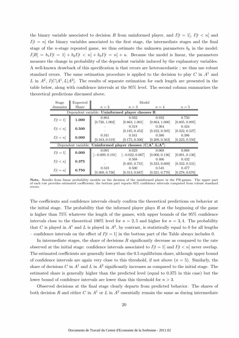
the binary variable associated to decision R from uninformed player, and I[t = 1], I[t < n] and

I[t = n] the binary variables associated to the first stage, the intermediate stages and the final

stage of the n-stage repeated game, we thus estimate the unknown parameters bk in the model:

I[R] = b1I[t = 1] + b2I[t < n] + b3I[t = n] + u. Because the model is linear, the parameters

measure the change in probability of the dependent variable induced by the explanatory variables.

A well-known drawback of this specification is that errors are heteroscedastic ; we thus use robust

standard errors. The same estimation procedure is applied to the decision to play C in A1 and

L in A2, I[C|A1, L|A2]. The results of separate estimation for each length are presented in the

table below, along with confidence intervals at the 95% level. The second column summarizes the

theoretical predictions discussed above.

Stage Expected Modeldummies Share n = 2 n = 3 n = 4 n = 5

Dependent variable: Uninformed player chooses R

I [t = 1] 1.0000.864 0.932 0.932 0.750

[0.726, 1.002] [0.863, 1.001] [0.864, 1.000] [0.605, 0.895]

I [t < n] 0.500– 0.318 0.364 0.424– [0.185, 0.452] [0.222, 0.505] [0.322, 0.527]

I [t = n] 0.0000.341 0.341 0.386 0.386

[0.163, 0.519] [0.175, 0.506] [0.209, 0.563] [0.223, 0.550]

Dependent variable: Uninformed player chooses (C|A1,L|A2)

I [t = 1] 0.0000.091 0.023 0.068 0.068

[−0.009, 0.191] [−0.022, 0.067] [0.000, 0.136] [0.001, 0.136]

I [t < n] 0.375– 0.568 0.466 0.432– [0.405, 0.731] [0.323, 0.609] [0.332, 0.531]

I [t = n] 0.7500.523 0.500 0.545 0.477

[0.309, 0.736] [0.313, 0.687] [0.321, 0.770] [0.278, 0.676]

Note. Results from linear probability models on the decision of the uninformed player in the PR-games. The upper partof each row provides estimated coefficients; the bottom part reports 95% confidence intervals computed from robust standarderrors.

The coefficients and confidence intervals clearly confirm the theoretical predictions on behavior at

the initial stage. The probability that the informed player plays R at the beginning of the game

is higher than 75% whatever the length of the games, with upper bounds of the 95% confidence

intervals close to the theoretical 100% level for n = 2, 5 and higher for n = 3, 4. The probability

that C is played in A1 and L is played in A2, by contrast, is statistically equal to 0 for all lengths

– confidence intervals on the effect of I[t = 1] in the bottom part of the Table always includes 0.

In intermediate stages, the share of decisions R significantly decrease as compared to the rate

observed at the initial stage: confidence intervals associated to I[t = 1] and I[t < n] never overlap.

The estimated coefficients are generally lower than the 0.5 equilibrium share, although upper bound

of confidence intervals are again very close to this threshold, if not above (n = 5). Similarly, the

share of decisions C in A1 and L in A2 significantly increases as compared to the initial stage. The

estimated share is generally higher than the predicted level (equal to 0.375 in this case) but the

lower bound of confidence intervals are lower than this threshold for n > 3.

Observed decisions at the final stage clearly departs from predicted behavior. The shares of

both decision R and either C in A1 or L in A2 essentially remain the same as during intermediate

20


Figure 9: Relative frequency of the stage-dominant action from informed subjects

50

75

100

NR−NoInfo NR PR FR

1 2 3 4 5 1 2 3 4 5 1 2 3 4 5 1 2 3 4 5

50

75

100

NR−NoInfo NR PR FR

2 3 4 5 2 3 4 5 2 3 4 5 2 3 4 5

(a) Last stage (b) Intermediate stages

Note. For each treatment and each length, the figures display the mean share of the informed player’s stage-dominant actions,in the final stage (left-hand side) and in intermediate stages (right-hand side).

stages – confidence intervals on I[t < n] and I[t = n] largely overlap.

We now turn to a less aggregated analysis of behavior underlying such correlation patterns:

when and to what extent the informed player reveals information; and the uninformed player

reacts to observed decisions.

5.2.1 Informed player’s behavior: Use of information

The three experimental treatments are labelled according to the expected amount of information the

informed player should use. However, as shown in Appendix A, the resulting local strategies at each

stage may still finely depend on the history of the game. Given the range of lengths we study, this

leads to an intractably large set of theoretical predictions. We circumvent this issue by focusing on

the properties of informed players’ decisions at the current stage only, independently of the history.

We define Bj,i,t as the dummy variable indicating whether the decision of the informed player j, in

stage t = 1, ..., n of game i = 1, ..., 20, is the stage-dominant decision: Bj,i,t = 1[T |A1, B|A2]. Thus,

B.,.,t = 1 for a fully revealing (stage-dominant) strategy; B.,.,t = 1/2 for a non-revealing strategy

(pure randomization between the two actions) and B.,.,t = 0 for a fully “counter-revealing” (stage-

dominated) strategy.

Figure 9 provides a coarse summary of how information is used in each treatment. Recall that

all treatments have one prediction in common: the informed player has nothing to loose in using

his private information (i.e., playing the stage-dominant action) at the last stage of the game. We

thus separate the figures according to the stage inside each game: the last stage of all games is

reported on the left-hand side, intermediate stages of all repeated games (in stages t = 1 to t = n−1

for all n > 1) are reported on the right-hand side. From both the left-hand side figure and the

frequency of the stage-dominant action observed in the FR- and PR-games, experimental subjects

21


unambiguously manage to use information whenever it’s worth using. The relative frequency of the

stage-dominant action in the FR-games ranges from 94% (first stage of the 5-stage repeated game)

to 100% (in a vast majority of the FR-games, with the exception of t = 1|n = 1 and t = 1, 2|n = 3).

In the PR-games, information is used to its expected extent: in long games (n > 2) the relative

frequency of the stage-dominant action always remains very close to the 75% theoretical level in

intermediate stages (from 65% in t = 4|n = 5 to 88% in t = 1|n = 4). In the two-stage PR-game

this relative frequency is much higher at every stage of the game, which is compatible with the

(multiple) equilibrium predictions (according to which the stage-dominant action is played with

probability between 75% and 100% in the first stage). In the last stage of the NR-games, the

stage-dominant action is played more than 95% of the time. Thus, experimental subjects optimally

adjust their use of information not only as a reaction to experimental treatments, but also along

the path of decisions over stages of a given game.

Support. The results described above are supported statistically. To get confidence intervals on

the share of decisions from the informed player which are the stage-dominant action in each stage,

we specify linear in probability models on the average of B = 1[T |A1, B|A2] over repetitions of the

same game by the same pair of subjects. We estimate separate OLS regressions for each treatment

and each length: Bi,t = b11[t = 1] + .... + bn1[t = n] + ui,t, n = 1, ..., 5, on data averaged at the

pair-length level. We estimate robust standard errors to account for the induced heteroskedasticity.

n = 1 n = 2 n = 3 n = 4 n = 5Stage (t) 1 1 2 1 2 3 1 2 3 4 1 2 3 4 5

NR-NoInfo 0.51 0.57 0.55 0.56 0.53 0.53 0.57 0.53 0.51 0.49 0.49 0.52 0.45 0.43 0.57Lower B. 0.41 0.46 0.44 0.46 0.44 0.44 0.48 0.44 0.42 0.39 0.38 0.41 0.33 0.31 0.49Upper B. 0.61 0.68 0.67 0.66 0.62 0.63 0.67 0.62 0.60 0.59 0.60 0.63 0.57 0.55 0.65

NR 0.97 0.89 0.98 0.79 0.87 0.95 0.73 0.73 0.89 0.98 0.58 0.71 0.74 0.85 0.98Lower B. 0.94 0.82 0.94 0.71 0.81 0.92 0.63 0.65 0.84 0.95 0.48 0.61 0.66 0.78 0.95Upper B. 1.00 0.95 1.01 0.87 0.93 0.99 0.84 0.82 0.95 1.00 0.67 0.81 0.82 0.92 1.00

PR 0.95 0.93 0.89 0.77 0.75 0.93 0.89 0.80 0.73 0.82 0.80 0.75 0.73 0.66 0.91Lower B. 0.89 0.86 0.75 0.65 0.60 0.86 0.81 0.67 0.56 0.63 0.68 0.62 0.62 0.51 0.83Upper B. 1.01 1.00 1.02 0.90 0.90 1.00 0.96 0.92 0.90 1.01 0.91 0.88 0.83 0.81 0.98

FR 0.98 1.00 1.00 0.98 0.96 1.00 1.00 1.00 1.00 1.00 0.94 1.00 1.00 1.00 1.00Lower B. 0.94 1.00 1.00 0.94 0.90 1.00 1.00 1.00 1.00 1.00 0.85 1.00 1.00 1.00 1.00Upper B. 1.02 1.00 1.00 1.02 1.01 1.00 1.00 1.00 1.00 1.00 1.03 1.00 1.00 1.00 1.00

Note. Results from OLS regressions on the decision of the informed player to play the stage-dominant action. An observationis the average for each pair over the four repetitions of the same game. For each treatment, the upper part of the row providesestimated coefficients; the two subsequent rows gives the lower and upper bounds of 95% confidence intervals computed formrobust standard errors.

In instances in which the informed player should fully use private information (FR-games and

last stage in all treatment) the 95% confidence intervals are close to the expected 100% share of

stage-dominant actions. There is much less dispersion, though, in the FR-games – in which the

optimal share always remains the same – than in the last stages of other games. In intermediate

stages of long PR-games (i.e., n > 2 and t < n), the confidence intervals gather proportions that are

always higher than 50% and lower than 100% ; in most cases, the prediction that 75% of decisions

are the stage-dominant actions is inside the confidence interval.

22


Figure 10: Relative frequency of the stage-dominant action from informed subjects, by stage

.5

.75

1

1 2 3 4 5

n=1 n=2 n=3

n=4 n=5 .5

.75

1

1 2 3 4 5

n=1 n=2 n=3n=4 n=5

(a) NR treatment (b) PR treatment

Note. For each stage in abscissa, the dots give the mean share of informed player’s decisions that are the stage-dominantaction of the game actually played. All stages from a given length (see the legend) are connected.

The ability of experimental subjects to optimally ignore information is much weaker. As an

empirical benchmark, Figure 9 reports observations from the NR-NoInfo treatment, in which neither

the row player nor the column player is informed of the actual payoff matrix. We do observe some

noise in this treatment: the relative frequency of the stage-dominant action ranges from 43% to

57%. In the NR-games, informed subjects should theoretically behave (almost) as in the NR-NoInfo

treatment, i.e., they should ignore their private information and play each action with probability

close to 50%. Contrasting these frequencies between the two treatments unambiguously suggests

decisions are too much correlated with information: the relative frequencies of the stage-dominant

actions we elicit in intermediate stages of the NR-games dominate those observed in NR-NoInfo,

and are very often similar to those observed in the PR-games. Still, these frequencies remain lower

than in both the FR-games and final stages of the NR-games.

While experimental subjects over-use their information in the NR-games, their strategy qual-

itatively reacts in the expected way to changes in the environment. Figure 10 disaggregates the

relative frequency of the stage-dominant action according to each stage inside the n-stage repeated

games. The cost of an excessive use of the stage-dominant strategy is that the uninformed player

becomes more and more able to play his perfectly informed decision and thus to get a higher share

of the total payoff in subsequent repetitions of the game. Clearly, the cost of revealing information

is increasing in the number of stages towards the end of the current game; that is, it is higher

if information is revealed earlier in the game for a given length, and it is higher if information is

revealed in longer games for a given stage. Figure 10 confirms that informed subjects adjust their

use of information according to those parameters. The relative frequency of the stage-dominant

action in stage t is decreasing in the total number of stages, n, for every stage t, and increasing

in t for every length n of the game. As a result, the amount of information transmitted through

decisions is fairly constant across games as regards the number of remaining stages. This consti-

23


tutes an important difference with behavior in the PR-games, in which the relative frequency of

the stage-dominant action is slightly decreasing in t in intermediate stages of all games.

Support. We provide statistical support to the qualitative variations in the use of information

through probit regressions on the probability that the informed player uses the stage-dominant

action. This led us to work at the game level, considering each play of a given length as one

observation. To account for multiple observations from the same pair of subjects, the regressions

include pairs dummies and round dummies – which identifies the order of the game among the 20

played by each pair. For both the NR-games and the PR-games, we estimate two specifications:

the first model includes only the effect of the length (n) and the stage (t), the second one isolates

the last stage of the game.

NR treatment PR treatment(1) (2) (1) (2)

Coef. p-value Coef. p-value Coef. p-value Coef. p-value

Constant 1.36 0.007 1.15 0.026 1.92 0.017 1.12 0.175n -0.47 0.000 -0.38 0.001 -0.27 0.351 0.05 0.870t 0.42 0.000 0.31 0.000 0.03 0.629 -0.15 0.055Final – – 0.57 0.000 – – 0.67 0.001

Nb Obs. 1798 638

Note. Probit regressions of the probability that the informed player uses the stage-dominant action on the stage(t) and the length (n) of the game (Models 1) as well as the dummy variable I[t = n] isolating the last stage ofthe game (Models 2). All models include pairs dummies and round dummies. P-values are comuted according torobust standard errors.

For the NR-games, the use of information is significantly decreasing in n and increasing in t even

when the last stage of each game is separated from intermediate stages (model 2). For the PR-

games, the use of information is constant across different lengths. Once the final stage is identified

separately, the use of information appears to decrease with the stage.

To sum up, information is accurately used when it should by informed players ; and the use of

information qualitatively reacts in the expected ways to changes in the environment. But subjects

experience difficulties in behaving as if they were uninformed. We now turn to the ability of

uninformed subjects to account for such revelation pattern.

5.2.2 Uninformed player’s behavior: rent extraction

We now assess whether uninformed subjects accurately react to informed subjects’ decisions. To

that end, we look at the average payoff of the uninformed player – which is a measure of the rent he

extracts from the informed player – as a function of the informed player’s past decisions. Table 4

summarizes this measure for each treatment, organized according to the informational content of

the informed player’s decisions.

Payoffs cannot be compared across treatments but variations in the payoffs have the same inter-

pretation in all treatments. The right-hand side (left-hand side) of the table aggregates the payoff

of the uninformed player that follow the play of the stage-dominant (stage-dominated) action from

24


Table 4: Uninformed players’ extraction of the information rent

Dominated action at previous stage Dominant action at previous stage OverallHistory index 0 1/3 .5 1 Total 0 1/3 .5 1 Total

FR-games: uninformed player’s payoff (Nb. obs.)

Dominated – – – 4.500 4.500 – – – – – 4.500most often (0) (0) (0) (4) (4) (0) (0) (0) (0) (0) (4)

Dominant 4.000 – – – 4.000 5.000 6.000 6.000 5.845 5.840 5.832most often (2) (0) (0) (0) (2) (4) (3) (3) (464) (474) (476)

NR-games: uninformed player’s payoff (Nb. obs.)

Dominated – 4.000 6.667 3.836 3.904 – 5.263 5.000 – 5.238 4.038most often (0) (25) (3) (159) (187) (0) (19) (2) (0) (21) (208)

Dominant 4.684 7.619 10.000 – 5.524 6.220 6.907 7.381 8.529 8.034 7.797most often (79) (21) (5) (0) (105) (127) (97) (42) (741) (1007) (1112)

PR-games: uninformed player’s payoff (Nb. obs.)

Dominated – 5.571 1.800 1.909 2.357 – 3.000 – – 3.000 2.379most often (0) (7) (5) (44) (56) (0) (2) (0) (0) (2) (58)

Dominant 3.130 4.750 4.000 – 3.732 4.125 5.077 5.700 4.967 4.953 4.822most often (23) (12) (6) (0) (41) (16) (13) (10) (302) (341) (382)

Note. Each cell provides the average payoff of the uninformed player, which measures the accuracy of the uninformed player’sdecision with respect to the actual stage game. Right-hand side (left-hand side): payoffs of the uninformed player that follow theplay of the stage-dominant (stage-dominated) action from the informed player, i.e., 1[R|A1, L|A2] = 1(= 0). For each treatment,the upper (bottom) row of the contains payoffs of the uninformed player that follow a majority of stage-dominant (stage-dominated) actions – i.e., the share of stage-dominant actions among all previous stages decisions is ≥ (<) 50%. In each row,the first figure refers to the uninformed player’s payoff and the second refers to the number of observations. Each column refersto the homogeneity of decisions observed in past stages, through the absolute value of the mean of 1[R|A1, L|A2]−1[L|A1, R|A2].N = 480(= 40 ∗ 12) in the FR-games, N = 1320(= 40 ∗ 33) in the NR-games, N = 440(= 40 ∗ 11) in the PR-games.

the informed player. For each treatment, the upper (bottom) row contains average payoffs of the

uninformed player that follow a weak (strong) majority of stage-dominant (stage-dominated) ac-

tions from the informed player. In each column, we further separate observed decisions according

to the homogeneity of decisions observed in past stages, through the absolute value of the mean

of 1[R|A1, L|A2] − 1[L|A1, R|A2]. This measure is closer to 1 (0) the more homogeneous (hetero-

geneous) is the observed history. The comparison between top and bottom rows thus provides

evidence on the effect of the history of decisions from the informed player; while comparisons be-

tween the left-hand side and right-hand side figures isolate the effect of the decision observed at

the previous stage. Last, comparisons across columns show the variation of the accuracy of the

uninformed player’s decision according to the correlation across stages of the informed player’s deci-

sions. In each game, this information is available starting at stage 2. We thus have 10 observations

per sequence of 5 games in each treatment – i.e.,∑5

n=2(n − 1) – resulting in 40 observations for

each uninformed player.

The individual behavior of the informed players in the FR-games is very concentrated on the

equilibrium path. There are extremely few observations for which the history of decisions is not

a perfectly homogeneous play of the stage-dominant action (only 16 observations out of the 480

available). In the NR-games, as expected from the theoretical predictions, empirical decisions from

informed players give rise to much more heterogeneity in the history. On average, the payoff of

the uninformed player falls from 7.8 to 4.0 when the dominated action rather than the dominant

25


one is observed most often in the past. The guesses appear more accurate when the dominant

action is observed most often, though. In this case (bottom row of the middle of the table),

the payoff is higher when the dominant action is the decision observed at last stage (from 5.5 to

8.0), and monotonically increases in the homogeneity of the history: the higher the history index

following either the stage-dominant or the stage-dominated action, the higher the payoff. When

the dominated action was observed most often in the past (top row of the middle part of the table),

by contrast, the last stage decision and the homogeneity of the history make very little difference

– the payoff varies from 3.8 to 6.7 according to the last stage decision, and no clear pattern appear

according to the history index.

The picture is very similar, although less clear-cut, in the PR-games. Whatever the last stage

decision and the content of the history, the uninformed player tends to take more into account

homogeneous histories. This results in a decrease of the rent extracted according to the history

index when the dominated action is both the most often observed and the last stage decision (from

5.6 to 1.9). When the dominant action prevails in the observed history, the rent increases with the

homogeneity index, from 3.1 to 4 when the last stage decision is the dominated action ; from 4.1

to 5.7 when the last stage decision is the dominant action. As a result, the average rent earned by

the uninformed player is higher following both a better history for a given last stage decision and

a better last stage decision for a given history (the majority decision induces an increase from 2.4

to 3.7 following a dominated action; from 2.4 to 4.8 following a stage-dominant action).

From these observations it appears that uninformed players do use several dimensions of the

history to make their decisions: the information content of the last decision and the nature and

homogeneity of the whole history. This allows them to account for the over-use of information in

the NR-games.

6 Conclusion

Zero-sum repeated games with incomplete information are a very clean environment to study the

use of information, and the value of being informed in strategic interactions. In such games, one

player is informed of the actual state of nature in which the whole game is played, the other is

not. Actions, but not payoffs, are observed from one stage to the other in the repeated game.

When a different action is dominant in each state of nature of the stage game, the stage-dominant

strategy of the informed player is a fully revealing signal of the state. Because players’ interest

are diametrically opposed, the uninformed player becomes able to capture the whole information

rent once he becomes informed of the actual stage. Depending on the stakes and the length of

the game, the informed player must solve the trade-off between the short term benefit of using

private information, and the long term opportunity cost of sharing it with the uninformed player.

The optimal balance between the two provides precise predictions on the shape and level of the

value of information – i.e., the expected payoff from being informed of the actual state against an

uninformed opponent.

This paper investigates the empirical content of the theoretical predictions associated with this

26


class of games. We study three payoff structures that differ according to the amount of information

the informed player should exploit: information should be fully used in the FR-games, partially

used in the PR-games and disregarded in the NR-games. For each payoff structure, we vary the

length of the repeated game from 1 stage to 5. From an experimental point of view, the NR- and

FR-games only differ according to the payoff associated to each action. In the PR-games, the set

of actions for the uninformed player is larger (three actions instead of two in the two other games).

We find strong support in favor of the theory in all three types of games. The empirical value of

information is in line with both quantitative and qualitative predictions. We reject, in particular,

that the value of information becomes negative in long games in which information should be

disregarded. What is more, in every treatment and whatever the lengths of the repeated games,

the average value of information in the lab is always bounded below by the theoretical value of

the infinitely repeated game. As regards individual behavior, the available information is used too

often when it should be ignored, but experimental subjects do not suffer from a curse of knowledge

because the use of information reacts in the expected way to the length and payoff structure of

the game. It would be interesting to investigate the robustness of these results by implementing

alternative competitive games with incomplete information in the laboratory.

References

Aumann, R. J. and S. Hart (2003): “Long Cheap Talk,” Econometrica, 71, 1619–1660.

Aumann, R. J. and M. Maschler (1966): “Game Theoretic Aspects of Gradual Disarmament,” Report

of the U.S. Arms Control and Disarmament Agency, ST-80, Chapter V, pp. 1–55.

——— (1967): “Repeated Games with Incomplete Information: A Survey of Recent Results,” Report of the

U.S. Arms Control and Disarmament Agency, ST-116, Chapter III, pp. 287–403.

Aumann, R. J. and M. B. Maschler (1995): Repeated Games of Incomplete Information, Cambridge,

Massachusetts: MIT Press.

Camerer, C., G. Loewenstein, and M. Weber (1989): “The Curse of Knowledge in Economic Settings:

An Experimental Analysis,” Journal of Political Economy, 97, 1232–54.

Cripps, M. and J. Thomas (2003): “Some asymptotic results in discounted repeated games of one-sided

incomplete information,” Mathematics of Operations Research, 433–462.

Feltovich, N. (1999): “Equilibrium and Reinforcement Learning in Private-Information Games: An Ex-

perimental Study,” Journal of Economic Dynamics and Control, 23, 1605–1632.

——— (2000): “Reinforcement-Based vs. Belief-Based Learning Models in Experimental Asymmetric-

Information Games,” Econometrica, 68, 605–641.

Forges, F. and F. Koessler (2008): “Long Persuasion Games,” Journal of Economic Theory, 143, 1–35.

Goltsman, M., J. Horner, G. Pavlov, and F. Squintani (2009): “Mediation, Arbitration and Nego-

tiation,” Journal of Economic Theory, 144, 1397–1420.

27


Greiner, B. (2004): “An Online Recruitment System for Economic Experiments.” in Forschung und wis-

senschaftliches Rechnen 2003. GWDG Bericht 63, ed. by K. Kremer and V. Macho, Gottingen: Ges. fur

Wiss. Datenverarbeitung, 79–93.

Hart, S. (1985): “Nonzero-Sum Two-Person Repeated Games with Incomplete Information,” Mathematics

of Operations Research, 10, 117–153.

Kamenica, E. and M. Gentzkow (2009): “Bayesian persuasion,” American Economic Review, forthcom-

ing.

Krishna, V. and J. Morgan (2004): “The Art of Conversation: Eliciting Information from Experts

through Multi-Stage Communication,” Journal of Economic Theory, 117, 147–179.

Loewenstein, G., D. Moore, and R. Weber (2006): “Misperceiving the value of information in pre-

dicting the performance of others,” Experimental Economics, 9, 281–295.

Lovo, S. and J. Horner (2009): “Belief Free Equilibria in Games of Incomplete Information,” Economet-

rica, 77, 453–487.

Mertens, J., S. Sorin, and S. Zamir (1994): Repeated Games, CORE DP # 9420, 9421, 9422.

Obara, I. (2009): “Folk Theorem with Communication,” Journal of Economic Theory, 144, 120–134.

Renault, J. and T. Tomala (2004): “Communication Equilibrium Payoffs in Repeated Games with

Imperfect Monitoring,” Games and Economic Behavior, 49, 313–344.

Sorin, S. (2002): A First Course on Zero-Sum Repeated Games, Springer.

Stearns, R. (1967): “A Formal Information Concept for Games with Incomplete Information,” Report of

the U.S. Arms Control and Disarmament Agency, ST-116, Chapter IV, pp. 405–433.

Zamir, S. (1992): “Repeated Games of Incomplete Information: Zero-Sum,” in Handbook of Game Theory,

ed. by R. J. Aumann and S. Hart, Elsevier Science B. V., vol. 1, chap. 5, 109–154.

28


Appendix

A Detailed equilibrium strategies for the NR-games

Denote pt player 2’s posterior belief about the state in stage t, t = 1, . . . , n, yt(ht−1) the strategy (probability

of playing L) of player 2 in stage t given the history of actions ht−1 ∈ {T,B}t−1 of player 1, and x1t (pt) and

x2t (pt) the strategy (probabilities of playing T in A1 and A2) of player 1 in stage t given the posterior pt of

player 2 in stage t. In the following tables, we describe the optimal strategies ((x1t , x

2t ), yt) and player 2’s

theoretical posteriors pt for the NR-games. In the NR-games, the recursive formula of Proposition 1 simplifies

to

vn+1(p) =10

n+ 1max

(x1,x2)∈[0,1]2min

y∈[0,1](px1y + (1− p)(1 − x2)(1 − y) + n

(αvn

(px1

α

)+ (1− α)vn

(p(1− x1)

1− α

))),

=10

n+ 1max

(x1,x2)∈[0,1]2px1 if px1 ≤ (1− p)(1− x2)

(1− p)(1− x2) if px1 ≥ (1− p)(1− x2)+ n

(αvn

(px1

α

)+ (1− α)vn

(p(1 − x1)

1− α

)) ,

where α = px1 + (1− p)x2 is the probability that player 1 plays T .

In G1(1/2), we thus have:

t ht−1 x1t x2

t pt yt

1 ∅ 1 0 1/2 1/2

In G2(1/2):

t ht−1 x1t x2

t pt yt

1 ∅ 1/2 1/2 1/2 1/2

2 T 1 0 1/2 1/4

B 3/4

In G3(1/2):

t ht−1 x1t x2

t pt yt

1 ∅ 1/2 1/2 1/2 1/2

2 T 1/2 1/2 1/2 1/2

B

3 TT 1 0 1/2 0

TB 1/2

BT

BB 1

29


In G4(1/2):

t ht−1 x1t x2

t pt yt

1 ∅ 4/7 3/7 1/2 1/2

2 T 1/2 1/3 4/7 3/7

B 2/3 1/2 3/7 4/7

3 TT 1/2 0 2/3 5/14

TB 1/2 1/2 1/2 1/2

BT

BB 1 1/2 1/3 9/14

4 TTT 1 0 1 0

BTT 1/2 3/14

TBT 2/7

TTB 5/14

BBT 9/14

BTB 5/7

TBB 11/14

BBB 0 1

30


In G5(1/2):

t ht−1 x1t x2

t pt yt

1 ∅ 1/2 1/2 1/2 1/2

2 T 4/7 3/7 1/2 7/16

B 9/16

3 TT 1/2 1/3 4/7 41/112

BT 55/112

TB 2/3 1/2 3/7 57/112

BB 71/112

4 TTT 1/2 0 2/3 13/56

BTT 27/56

TTB 1/2 1/2 1/2 1/2

TBT

BTB

BBT

TBB 1 1/2 1/3 29/56

BBB 43/56

5 TTTT 1 0 1 0

BTTT

TTTB 1/2 13/56

TTBT 11/112

TTBB 67/112

TBTT 3/112

TBTB 59/112

TBBT 29/56

BTTB 27/56

BTBT 53/112

BTBB 109/112

BBTT 45/112

BBTB 101/112

BBBT 43/56

TBBB 0 1

BBBB

31
