USING NUMERICAL TECHNIQUES TO

ACCELERATE DELAYED ETTRINGNITE

FORMATION TEST METHODS

By

JOHN BRET ROBERTSON

Bachelor of Science in Civil Engineering

Oklahoma State University

Stillwater, Oklahoma

2008

Submitted to the Faculty of the Graduate College of the

Oklahoma State University in partial fulfillment of

the requirements for the Degree of

MASTER OF SCIENCE May, 2010

ii

USING NUMERICAL TECHNIQUES TO

ACCELERATE DELAYED ETTRINGNITE

FORMATION TEST METHODS

Thesis Approved:

Tyler Ley, Ph.D., PE

Thesis Adviser

John N. Veenstra, Ph.D., PE, BCEE

Robert N. Emerson, Ph.D., PE

A. Gordon Emslie, Ph.D.

Dean of the Graduate College

.

iv

ACKNOWLEDGMENTS

I would like to thank my wife, Tara, for being patient while I have been in school and for

the continual encouragement. I would like to thank my grandparents, Clay and Betty, for

this opportunity to pursue my Masters degree. I would like to thank my parents, Rob,

Brenda, Roberta, and Dale, for the continued support. I would also like to thank Dr.

Tyler Ley for the opportunity to work with him for my undergraduate and graduate

degrees. I am grateful to have met you and been able to work with you over the last few

years. I would like to thank Dr. John Veenstra for his guidance in both undergraduate

and graduate school. I would also like to thank Dr. Robert Emerson for his guidance

during undergraduate and graduate study.

v

TABLE OF CONTENTS

LISTOFTABLES ........................................................................................................... vi

LISTOFFIGURES ........................................................................................................ vii

I.THESISINTRODUCTION............................................................................................. 11.1Introduction ................................................................................................................... 1

II.USEOFSORENSENANDDERIVATIVEMETHODSTODETERMINETHEULTIMATEEXPANSIONOFSPECIMENSFROMDEF ........................................................................ 32.1 Introduction ............................................................................................................... 32.2 Methodology.............................................................................................................. 52.3 FittinganS‐CurvetoData ........................................................................................... 82.4 SorensenMethod..................................................................................................... 102.5 DerivativeMethod ................................................................................................... 132.6 Results ..................................................................................................................... 152.7 Discussion ................................................................................................................ 192.8 Conclusion................................................................................................................ 19

III.DEFTESTING......................................................................................................... 213.1 Introduction ............................................................................................................. 213.2 Methods................................................................................................................... 253.3 ExpansionandWeightChangeresults ...................................................................... 303.4 Discussion ................................................................................................................ 313.5 Conclusion................................................................................................................ 32

IV.CONCLUSIONS ...................................................................................................... 334.1 UseofSorensenandDerivativeMethodstoDeterminetheUltimateExpansionofSpecimensfromDEF .......................................................................................................... 334.2 DEFTesting............................................................................................................... 34

REFERENCES .............................................................................................................. 35

APPPENDICES ............................................................................................................ 36A.1 Example1.FastAcceleratingCurve. ........................................................................ 36A.2 Example2.MediumAcceleratingCurve................................................................... 39A.3 Example3.SlowAcceleratingCurve. ....................................................................... 42

vi

LIST OF TABLES

Table2.1.UsedtodeterminethepercenterrorforthefinalexpansionusingthetctotlratiothatcontrolsthefittedcurveswhileutilizingthevariableA. .......................... 13

Table2.2.Sorensenmethodtestingresults. ............................................................. 17

Table2.3.Derivativemethodresults. ....................................................................... 18

Table3.1.Benicia‐MartinezBridgemixdesign........................................................... 22

Table3.2.Coreinformation(Maggenti2008)............................................................ 23

Table3.3.MixdesignfortheTexascores(McMillan,2009). ..................................... 25

vii

LIST OF FIGURES

Fig.1.1MultipleS‐curvesfromcommonASTMtests................................................... 2

Fig.2.1MultipleS‐curvesfromcommonASTMtests................................................... 3

Fig.2.2.Sorensenmethodshowngraphically. ............................................................ 6

Fig.2.3.Sorensengraphplottedfromthefittedcurve. ............................................... 6

Fig.2.4.Thederivativemethodshowngraphically. ..................................................... 7

Fig.2.5.ThederivativeoftheS‐curve. ........................................................................ 8

Fig.2.6.ThisfigureshowhowvariableAchangesthes‐curvemagnitudes.................. 9

Fig.2.7.Thisgraphshowshowvariabletlchangesthelatencyperiod. ....................... 9

Fig.2.8.VariabletcchangesthesteepnessoftheslopeoftheS‐curve...................... 10

Fig.2.9.Collecteddatathathasstartedtoaccelerate. .............................................. 12

Fig.2.10.ExtrapolatingfromtheSorensencurve. ..................................................... 12

Fig.2.11.Datacollectedforderivativemethod......................................................... 14

Fig.2.12.Thisfigureshowstheamountofdataneededtodeterminethemaximum.15

Fig.3.1.PictureoftheNewBeniciaBridge(Murugesh,2008). .................................. 23

Fig.3.2.ColumncoredfortheTexascores(McMillan,2009)..................................... 24

Fig.3.3.Layoutofthehowthecoreswerelabeledshippedandfordatarecording... 26

Fig.3.4.CoresA,B,C,andEweremeasuredinthreesegments. ................................ 27

Fig.3.5.Informationonlycast‐in‐placeblocksforcoringandtemperaturerecording................................................................................................................................... 28

Fig.3.6.Generaldemeclayoutforoneline. .............................................................. 29

Fig.3.7.ShowsthedifferencebetweencoreDandtheothercores. ......................... 29

Fig.3.8.Mayesgauge,7.9”inlength......................................................................... 30

Fig.3.9.Theexpansionmeasurementsforeachcore ................................................ 31

1

CHAPTER I

THESIS INTRODUCTION

1.1 Introduction

Construction materials deteriorate over time, often this process needs to be

monitored in order to evaluate the health of the structure. Unfortunately, it is often

impractical to measure this deterioration on actual structures due to the extended periods

that the deterioration takes place over. For this reason accelerated test methods have

been developed. These laboratory tests may not simulate the actual performance of these

materials but should provide a useful comparison between materials. Some of these tests

include: ASTM C 1260, 1293, 1012, 878, 227, and Delayed Ettringite Formation (DEF)

expansion tests. This thesis will present a numerical technique that can be used to

estimate the final results of tests with symmetric S-curves. S-curves consist of a constant

period with no reaction, followed by an acceleration period with a lot of reaction, and

ending with a constant period with no more reaction. As shown in Fig. 1.1, the results

from these tests resemble an S-curve. Despite attempts to accelerate some of these tests,

sometimes results can take up to 2 years for the reaction to be completed.

2

Fig. 1.1 Multiple S-curves from common ASTM tests

Also some test methods have a minimum and maximum value established to confirm if

the specimen has the proposed deterioration problem. The proposed technique has the

ability to decrease these test times by 50% or better, if the test has a symmetric S-curve.

This thesis will also cover lab testing of cores with potential DEF from bridge projects in

California and Texas. After the cores were received from the respected projects,

measuring points were attached and the samples were stored in water in a controlled

environment. The cores were measured for expansion and volume change over time.

00.20.40.60.81

1.21.41.61.82

0 25 50 75 100 125 150

Percen

tLen

gthCh

ange

Days

C1260

C1293

C227

DEF

3

CHAPTER II

USE OF SORENSEN AND DERIVATIVE METHODS TO DETERMINE THE

ULTIMATE EXPANSION OF SPECIMENS FROM DEF

2.1 Introduction

Several American Society Test Methods (ASTM) concrete durability tests have

results that have an S shape. Some examples of these tests include ASTM C 1260, 1293,

1012, 878, 227. Some results for these tests are shown in Fig. 2.1. In these tests concrete

is placed in different environments and the length change of the specimens are measured

over time.

Fig. 2.1 Multiple S-curves from common ASTM tests.

00.20.40.60.81

1.21.41.61.82

0 25 50 75 100 125 150

Percen

tLen

gthCh

ange

Days

C1260

C1293

C227

DEF

4

Despite attempts to accelerate these tests results can take up to 2 years for the reaction to

be completed and for the specimen to stop changing. Because of this it is common for

the tests to specify a limiting value at a certain point within the test. This allows one to

evaluate the results of the test before the completion of the reaction. These limiting

values are challenging to choose, but are based of engineering judgment or from limits

from the field performance of concretes. However, there are tests which no limiting

value is chosen such as the Fu DEF test (Fu, 1996) or when one is modifying a test to

evaluate field specimens such as the testing of cores from an actual structure in

“Investigation of the Internal Stresses Caused by Delayed Ettringite Formation in

Concrete,” by Burgher et al., 2008. In these cases the tests are run to completion, as they

measure the potential expansion for the specimen as there are no established

recommended values. This means potentially years later, a result will be determined.

This is not adequate for maintenance decisions for the field or the acceptance criteria of a

mixture.

Two different methods are presented that use numerical techniques to estimate the final

length change in the test. These methods have the ability to decrease these test times by

50% or better. The Sorensen method (Sorensen, 1951) was derived to be used with

titrations to help the investigator find the end point more exactly. In the other technique

derivatives of the data are used to find the inflection point and the final expansion. Both

methods are possible because of the y-symmetric aspects of the DEF expansion curves.

5

2.2 Methodology

The methodology used can be summarized with the following steps:

• Fit collected data to an S-curve

• Use Sorensen or derivative methods to find the inflection point

• Find y-value of inflection point and double it for final value

Symmetric S-curves have a constant period before accelerating then followed by

another constant period. Curve fitting should take place when the s-curve begins to

accelerate from the first constant period. After this acceleration begins the Sorensen

method can be used to predict the inflection point. The Sorensen method is shown

graphically in Fig. 2.2 and 2.3, below. Fig. 2.2 shows where the inflection point is in

respect to the entire set of data. The solid line shows the amount of data needed in order

to use the Sorensen method. Fig. 2.3 shows the Sorensen graph from the fitted curve.

This is then extrapolated down to the x-axis intercept. The intercept is the assumed

inflection point. These results are shown for test results for the Fu DEF test method;

however, the results can be used for test results from any y symmetric s-shapped curve.

6

Fig. 2.2. Sorensen method shown graphically.

Fig. 2.3. Sorensen graph plotted from the fitted curve.

The Sorensen method is able to estimate the inflection point almost immediately after the

slope of the curve starts to increase. By using the assumed x-value of the inflection point,

0

0.5

1

0 200 400 600

%Exp

Days

InflecAonPoint

CompletedTestData

DataneededfortheSorensenesAmaAon

0

0.5

1

0 200 400 600

10(‐%Exp)

Days

Sorensen

ExtrapolatedLine

AssumedInflecAonPoint

7

and interpolating with the x and y value of the last data point measured on the original S-

curve to obtain the inflection point y-value. This new y-value can then be doubled to

obtain the final expansion of the S-curve.

Alternatively, the derivative method can be used. Once the s-curve starts to accelerate

from the first constant period a curve can be fit to the data. A derivative of the fitted

curve is then plotted. One challenge with the derivative technique is that it requires that

half the test data be collected to get the inflection point of the curve whereas the Sorensen

method does not. The maximum of the derivative is equal to the inflection point. The y-

value from the actual data for the inflection day can then be doubled to obtain the final y-

value. The derivative method can be seen graphically below in Fig. 2.4 and 2.5.

Fig. 2.4. The derivative method shown graphically.

0

0.5

1

0 200 400 600

%Exp

Days

InflecAonPoint

CompletedTestData

DataneededfortheDerivaAveMethod

8

Fig. 2.5. The derivative of the S-curve.

2.3 Fitting an S-Curve to Data

The first step for the process is to take the test data and fit a curve to the data. A

smooth curve allows the accuracy of the methods to be improved. To fit the curve to the

data, the following equation will be used:

Y=A(1-e-t/tc)/(1+e-(t-(tl/tc)) (Equation 2.1)(Larive, 1998)

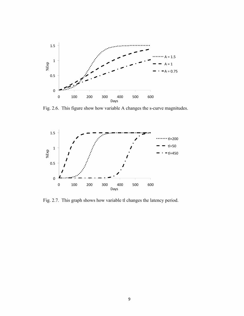
Where: Y= y-axis, representing %Exp t = time, represents the x-axis A= represents the maximum amplitude of the S-curve (final Expansion) tc = changes the slope of the S-curve, a larger number produces a slower accelerating curve, a smaller number produces a faster accelerating curve tl = determines the constant portion of the curve previous to the inflection point (larger number increases the length of the constant phase) The following graphs will show how each variable contributes to Larive’s equation.

0

0.001

0.002

0.003

0.004

0.005

0.006

0.007

0.008

0 200 400 600

∆(%

Exp)/∆(Days)

Days

DerivaAveofS‐curve

AssumedInflecAonPoint

ExtraData

9

Fig. 2.6. This figure show how variable A changes the s-curve magnitudes.

Fig. 2.7. This graph shows how variable tl changes the latency period.

0

0.5

1

1.5

0 100 200 300 400 500 600

%Exp

Days

A=1.5

A=1

A=0.75

0

0.5

1

1.5

0 100 200 300 400 500 600

%Exp

Days

tl=200

tl=50

tl=450

10

Fig. 2.8. Variable tc changes the steepness of the slope of the S-curve.

To fit the curve to the data, an iterative, graphical method is used. Plotting the data from

the S-curve then plotting data using eqn. 2.1. Comparison of the graphs should be at least

an R2 value of 0.95. This is the first step in both methods. Fitting a curve with a lower

time step increases the fitted s-curve accuracy and increases accuracy of the inflection

point for both proposed methods. As the Sorensen graph turns down towards the x-axis a

smaller time step on the fitted curve will decrease the error in the assumed inflection

point. A suggested time step for accurate results would be any value less than 5 days.

Also for the derivative method, the smaller time step will give a definitive maximum with

the least possible error.

2.4 Sorensen Method

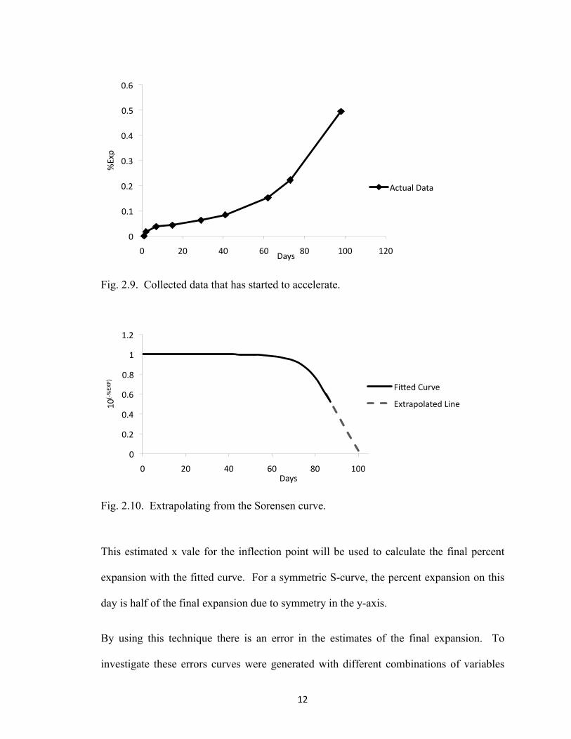
The Sorensen method can be used when the percent length change starts to

increase as shown in Fig. 2.9, the fitted S-curve should be made from the data. For any

0

0.5

1

1.5

0 100 200 300 400 500 600

%Exp

Days

tc=45

tc=150

tc=300

11

type of S-curve, one could check the slope of the curve. While the S-curve is in the first

constant period, the slope will be zero. Once the S-curve starts to accelerate, the slope

will begin to increase. The ratio of tc to tl should be calculated after fitting the curve to

the data. The tc to tl ratio has been found to correlate to the accuracy of the calculated

inflection point and the final percent expansion. Next the Sorensen plot is made using the

fitted data. The X-values will be time. The Y-values are calculated by the following

equation:

Y=10-%Exp (Equation 2.2)

When the data is plotted with the Sorensen method, the inflection point in the original

data is located by the point when the data crosses the X-axis. One benefit of this

technique is that one does not have to wait until the Sorensen plot reaches the X-axis as

the data is linear during the acceleration period. This allows the inflection point to be

estimated at a point much earlier in the test. This process is shown in Fig. 2.9 and 2.10.

Once this inflection point is found one can use interpolation the actual inflection point to

estimate the final expansion of the test. Since, the actual data S-curve will likely not be

to the real inflection point due to the Sorensen method finding the inflection point early,

interpolation can be used to find the expansion on the inflection day. This allows the

final expansion of the test to be estimated at a point that is much earlier than the

completion of the test.

12

Fig. 2.9. Collected data that has started to accelerate.

Fig. 2.10. Extrapolating from the Sorensen curve.

This estimated x vale for the inflection point will be used to calculate the final percent

expansion with the fitted curve. For a symmetric S-curve, the percent expansion on this

day is half of the final expansion due to symmetry in the y-axis.

By using this technique there is an error in the estimates of the final expansion. To

investigate these errors curves were generated with different combinations of variables

0

0.1

0.2

0.3

0.4

0.5

0.6

0 20 40 60 80 100 120

%Exp

Days

ActualData

0

0.2

0.4

0.6

0.8

1

1.2

0 20 40 60 80 100

10(‐%EXP)

Days

FiTedCurve

ExtrapolatedLine

13

and the error of the method quantified. These errors were found to be consistent between

the investigations with similar curve fit values. Because this error is similar between

investigations than a correction factor can be used on the predicted value based on the

fitted variables A, tl, and tc. Table 2.1 shows this relationship between s-curves with

common A values and multiple tc and tl values. Variable A controls the magnitude of the

s-curves and is also correlated with the percent error a curve will have using the Sorensen

method. Three A values were chosen with the values of 1, 1.5, and 2. The tc to tl ratios

chosen for the table were 0.1, 0.2, 0.3, 0.4, and 0.5. Interpolation to more specific values

of A and tc to tl can be made.

Table 2.1. Used to determine the percent error for the final expansion using the tc to tl ratio that controls the fitted curves while utilizing the variable A.

2.5 Derivative Method

This method provides a way to determine the final percent expansion by utilizing

the derivative of the fitted curve data near the inflection point of the graph. The

derivative is then taken of the fitted symmetric S shaped curve to make a parabolic graph.

This method is shown graphically in Fig. 2.11 and Fig. 2.12. The derivative of the fitted

curve can then be plotted by the change in the y variable with respect to the x variable.

This must be continued along with collecting data points until the derivative plot turns

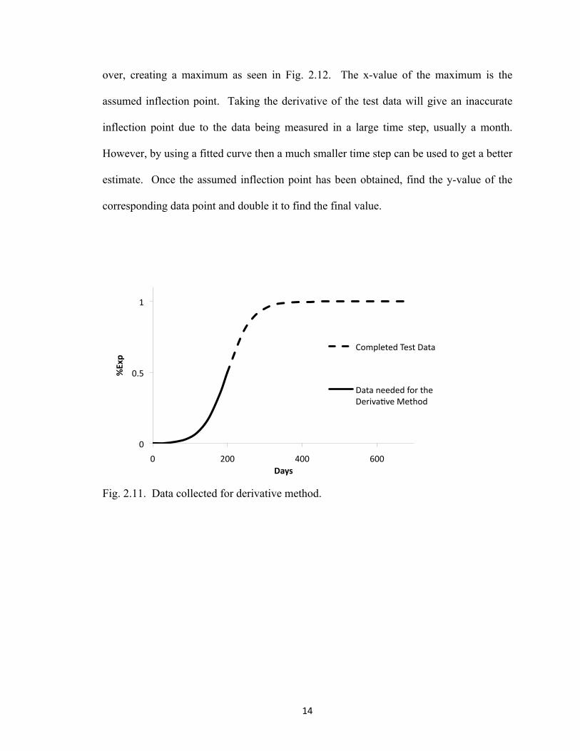
14

over, creating a maximum as seen in Fig. 2.12. The x-value of the maximum is the

assumed inflection point. Taking the derivative of the test data will give an inaccurate

inflection point due to the data being measured in a large time step, usually a month.

However, by using a fitted curve then a much smaller time step can be used to get a better

estimate. Once the assumed inflection point has been obtained, find the y-value of the

corresponding data point and double it to find the final value.

Fig. 2.11. Data collected for derivative method.

0

0.5

1

0 200 400 600

%Exp

Days

CompletedTestData

DataneededfortheDerivaAveMethod

15

Fig. 2.12. This figure shows the amount of data needed to determine the maximum.

2.6 Results

The Sorensen and Derivative methods were used with DEF test data. Each test

was plotted with percent expansion versus time. For the purposes of this method the test

data was only taken to where the curves start to accelerate (a slope change from the

constant period to the accelerating period), the rest of the data was not plotted or used

until after the final results were found. For the Sorensen method a curve was fit

graphically, using eq. 2.1, in an iterative process to get an R-squared of at least .95 with

the original data. After fitting the curve the Sorensen plot was made. The inflection

point was found from extrapolating from the steepest slope of the Sorensen curve to the

X axis. The steepest slope of the Sorensen curve, or the minimum of the derivative of the

Sorensen curve, will find the best extrapolation point to estimate the inflection point for

the fitted curve.

0

0.001

0.002

0.003

0.004

0.005

0.006

0.007

0.008

0 200 400 600

∆(%

Exp)/∆(Days)

Days

DerivaAveofS‐curve

ExtraData

16

Once the inflection point is found from the Sorensen extrapolation one can use

interpolation to find the actual inflection point to estimate the final expansion of the test.

Since, the actual data will likely not be to the real inflection point, interpolation can be

used to find the expansion on the inflection day. Once the inflection day expansion is

found this value is doubled to obtain the final expansion. The final expansions from the

Sorensen method were compared to the actual data for accuracy and time saved, as seen

in table. 2.2. The final data point of the test data is assumed to be the final expansion of

the sample.

For the Derivative method results, the same process was used to fit the curve. Instead of

graphing the Sorensen, the derivative of the fitted curve was graphed and the x-value of

the maximum found. This maximum is the assumed inflection point. The same steps

were used as the Sorensen method results to obtain the final expansion after the assumed

inflection point was found. The final expansions were compared with the real data

expansions, for accuracy and time saved, as seen in table 2.3.

17

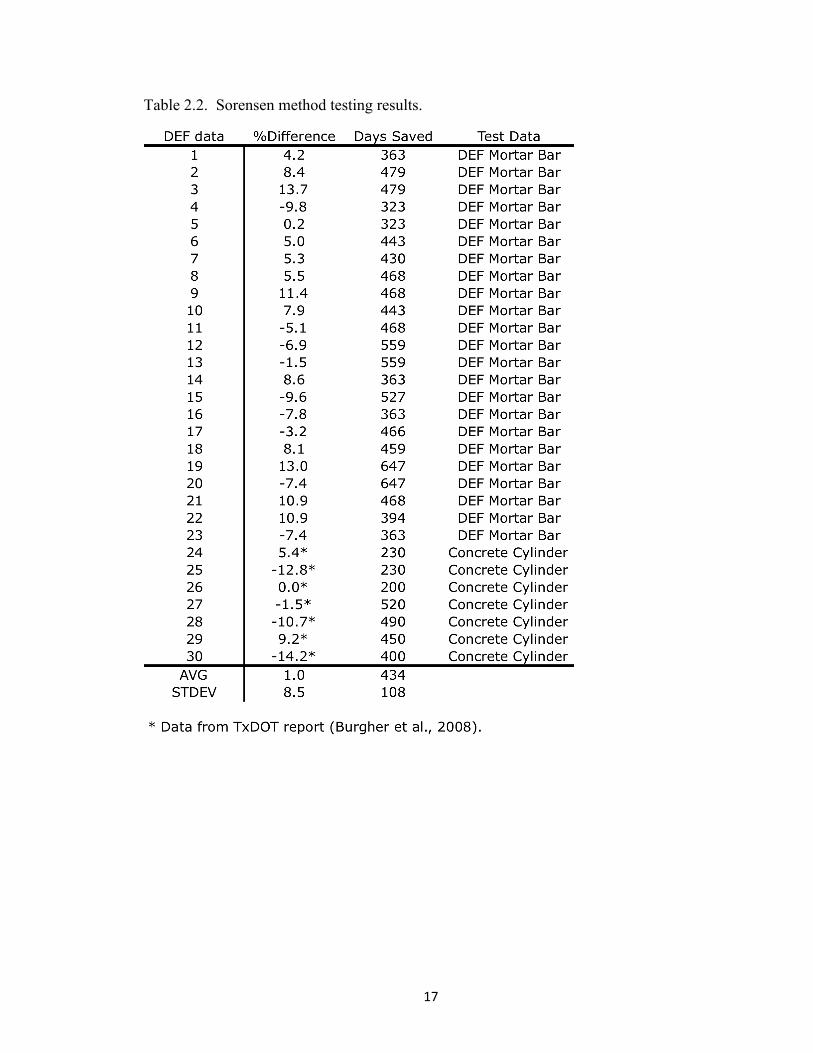
Table 2.2. Sorensen method testing results.

18

Table 2.3. Derivative method results.

19

2.7 Discussion

Using the Sorensen method allows early and accurate results for DEF expansion

testing. The Sorensen method shortened testing by an average of 434 days and with an

average of 1.0% difference and a standard deviation of 8.5% difference from actual final

expansions. This is a substantial improvement. Less than ten of the tests had a percent

difference above 10%. This could be improved by fitting the curve with a higher R-

squared value or by obtaining an additional data point. The Derivative method had the

same days saved as the Sorensen method due to using the same fitted curves but accuracy

was reduced. The average was -11.3% difference with a standard deviation of 23.9%

difference from the actual data. The fitted curves could made later with the Derivative

method to improve the accuracy. With the Sorensen and Derivative methods the DEF

expansion tests can be completed accurately and should not take more than 60% of the

normal test time.

2.8 Conclusion

DEF expansion tests should no longer take years to complete. This work has

shown that by using the Sorensen method close estimates of the final expansions can be

obtained while significantly shortening the testing period. This method was used on 30

different DEF tests and found to significantly shorten the testing period. This work will

help determine the expansion of laboratory tests or field data with a significant

improvement in speed. This would allow an owner to make a much quicker decision

about either maintenance of their structure or the ingredients in their mixture design.

20

Future work includes using these techniques with Y unsymmetrical s-curves similar to

ASTM C 1290 and 1260 results. Shrinkage may be included as well. The Sorensen

method was attempted with these types of S curves but was not consistent; however,

some modifications may be made.

21

CHAPTER III

DEF TESTING

3.1 Introduction

DEF is defined as the formation of ettringite after the concrete has hardened

(Taylor et al., 2001). Normally, ettringite forms during the curing process where the

concrete is still plastic and can accommodate the growth of ettringite without cracking.

The potential for DEF-induced distress occurs when the heat of the concrete during

hydration is above 160 oF. During hydration the ettringite becomes unstable and enters

the solution. The aluminate and sulfate ions rapidly become trapped in the rapidly

forming calcium silicate hydrates (C-S-H). Subsequent long-term exposure to moist

environments and a drop in pore solution pH leads to the release of these aluminate and

sulfate ions from the C-S-H. These ions then then react with monosulfate compound to

form ettringite. However, formation of ettringite in small pores in hardened concrete

cannot be accommodated by the rigid microstructure, and expansion and subsequent

cracking results (Burgher et al., 2008).

22

Cores were received with suspected DEF from the Benicia-Martinez Bridge located on I-

680, a 1.4-mile long bridge crossing the Carquinez Strait in Martinez, California as seen

in Fig 3.1. It was completed in 2007, in excess of $1 billion, with 335 cast-in-place,

lightweight concrete,single cell box girder segments with spans up to 660 feet and over

100 piles with diameters from 8 to 9 feet. The bridge is 82 feet wide with five lanes of

traffic. The bridge is built to withstand a maximum credible earthquake and provide a

future light rail. Lightweight concrete was used to construct the cast-in-place segments.

The concrete mixture proportions can be seen in table 3.1. Lightweight aggregate was

used to decrease the cost by increasing the span lengths according to feasibility study

performed in the 1980’s based on a 525 ft. span length (Murugesh, 2008).

Table 3.1. Benicia-Martinez Bridge mix design.

Lightweight concrete with normal weight sand was specified to achieve higher

compressive strength, higher modulus of elasticity, and less creep and shrinkage

(Murugesh, 2008). This high cementitious materials content lead to a high heat of

hydration. The construction specifications limited the maximum concrete temperature to

160°F (71°C) during curing. Multiple segments cast had thermocouple measurements

exceeding 160°F (71°C) with four of these exceeding 176°F (80°C). The highest

temperature recorded was 196°F (91°C) in a lightweight concrete segment soffit

(Maggenti and Brignano, 2008). The bridge was treated with a silane coating to try and

23

reduce the internal humidity of the concrete in hopes to prevent DEF as well as other

concerns. These cores will be referred to as the California cores.

Information about each core is shown in Table 3.2.

Table 3.2. Core information (Maggenti 2008).

Cores A,B Core C Core D Core E

Length (in) 26 28 23 14

Diameter (in) 2 3 3 3

Parts 2 2 2 1

Taken from 59 inch block 59 inch block 59 inch block 22 inch wall mockup

Temperature Reached 217˚F 217˚F 217˚F 163˚F

Fig. 3.1. Picture of the New Benicia Bridge (Murugesh, 2008).

Cores were also received from a bridge project in Lolaville, Texas. These will be

referred to as the Texas cores. Columns for the bridge were placed August 29, 2008.

The cores came from column B, in the northbound lane, bent #3, at Coit Road on SH 121

24

as seen in Fig 3.2, it was suspected of an internal temperature exceeding 160˚F. The

concrete mix proportions can be seen in Table 3.2

Fig. 3.2. Column cored for the Texas cores (McMillan, 2009).

25

Table 3.3. Mix design for the Texas cores (McMillan, 2009).

Two 2 inch diameter cores were 10 inches long, the other 10, 2 inch diameter cores were

broken into pieces and were not able to be evaluated. Two 4x8 inch cylinders were also

received with the Texas cores and used to measure expansion.

3.2 Methods

To measure the vertical expansion of the cores, demec points were mounted in three

lines arranged every 120 degrees around the circumference as seen in Fig. 3.2. This

method is similar to the method used in “Investigation of the Internal Stresses Caused by

Delayed Ettringite Formation in Concrete,” by Burgher et al., 2008. To mount the demec

points a two-part epoxy was applied to the concrete core at specified points. To measure

cores A, B, C, and E three lengths were measured as seen in Fig. 3.3. For the California

cores several test blocks that were cast to investigate the heat developed from different

mixture designs as seen in Fig. 3.4.

26

Fig. 3.3. Layout of the how the cores were labeled shipped and for data recording.

27

Fig. 3.4. Cores A,B, C, and E were measured in three segments.

28

Fig. 3.5. Information only cast-in-place blocks for coring and temperature recording.

The Texas cores were measured the same as core D from the California cores, because of

the 8 and 10 inch lengths. Core D and the Texas cores were only long enough to place 2

demec points per line around the core

To mount the demec points a two-part epoxy was applied to the concrete core at specified

points. Three lines of six points were arranged on all the cores except the two cores that

were shorter (core D and Texas cores), which has three lines of two demec points. The

demec layout for each kind of core can be seen in Fig. 3.6 and 3.7. A 7.9-inch Mayes

gauge, Fig. 3.8, was used to measure vertical distances for each core with a tolerance of

29

±0.00005 inches. The cores were also checked for volume change, which was recorded

each time the expansion was checked.

Fig. 3.6. General demec layout for one line.

Fig. 3.7. Shows the difference between core D and the other cores.

30

Fig. 3.8. Mayes gauge, 7.9” in length.

3.3 Expansion and Weight Change results

Expansion was measured multiple times in the first month and then periodically

after that. Fig. 3.9 shows the results of California and Texas core expansions with nearly

zero percent expansion after 560 days.

31

Fig. 3.9. The expansion measurements for each core

3.4 Discussion

The expansion results showed very little if any expansion in all of the California

cores. Correlation between the baseline core E and the other cores were consistent. A

delayed acceleration could still be a possibility but currently the cores show no signs of

DEF. This may be due to the fact that the cement used was a type II/V. Type V cement

by design has a low amount of C3A which contributes to the DEF expansion. Also the

DEF expansion could have taken place in the field since the cores were received in the

summer of 2008. The bridge was completed in the summer of 2007. The volume change

also stayed consistent, and was not measured after day 140. If a significant length change

occurs in future testing then these volume measurements will continue to be made.

0.00 0.05 0.10 0.15 0.20 0.25 0.30 0.35 0.40

0 100 200 300 400 500 600

%Ex

p

Days

Core Summary Core A-Top

Core A-Bottom

Core B-Top

Core B-Bottom

Core C-Top

Core C-Bottom

Core D-Top

Core D-Bottom

Core E

Texas Core 1

Texas Core 2

32

3.5 Conclusion

Cores were received with potential DEF. At this point in the testing no expansion

has occurred and so it does not appear that there is any potential for DEF in the concrete

that was sent for testing. Future work may include more expansion testing utilizing the

proposed method in this thesis.

33

CHAPTER IV

CONCLUSIONS

4.1 Use of Sorensen and Derivative Methods to Determine the Ultimate

Expansion of Specimens from DEF

This work took a couple of numerical methods and used them to shorten DEF

expansion tests. Each method has been presented in a way that is easy to use. After

proposing each method, thirty DEF expansion tests were randomly selected to utilize

both methods. Results from Sorensen method showed accurate findings decreasing test

times significantly. The Derivative method decreased test times the same as the Sorensen

method but was not as accurate due to the saved time. This work will help determine the

final expansion of DEF laboratory tests or field data with a significant improvement in

speed. This would allow an owner to make a much quicker decision about either

maintenance of their structure or the ingredients in their mixture design.

34

4.2 DEF Testing

Cores were received with potential DEF from a project in California and also a

project in Texas. Demec points were applied to the cores to use the Mayes gauge to

measure the expansion over time. The cores were then placed under water in a

temperature-controlled room, at 73˚F, to be measured periodically to record the percent

length change over time. To date none of the cores have shown enough expansion to

have DEF. Expansion checks will continue to take place to check for a delayed reaction

of DEF expansion.

35

REFERENCES

Burgher, B., Thibonnier, A., Folliard, K., Ley, T., and Thomas, M., “Investigation of the Internal Stresses Caused by Delayed Ettringite Formation in concrete,” FHWA/TX-09/0-5218-1, 2008.

Fu, Y., “Delayed Ettringite Formation in Portland Cement Products,” M.S. Thesis, University of Ottawa, 1996.

Larive, C., Apports combinés de l'expérimentation et de la modélisation à lacompréhensionde l'alcali-réaction et de ses effets mécaniques, Etudes et recherches des LPC. OA vol. 28 (1998).

Maggenti, R., and Brignano, B., Mass Concrete and the Benicia-Martinez Bridge, HPC Bridge Views, Issue 47, Jan/Feb 2008.

Maggenti, R., Personal Communication, 2008.

McMillan, B., Personal Communication, 2009.

Murugesh, M., Lightweight Concrete and the New Benicia-Martinez Bridge, HPC Bridge Views, Issue 49, May/June 2008.

Sorensen, P., Kem. Maanedsbl., 1951, 32

Taylor, H.F.W., Famy, C., Scrivener, K.L., ‘Delayed Ettringite Formation,’ Cement andConcrete Research, 31, 2001, pp. 683-693.

36

APPPENDICES

A.1 Example 1. Fast Accelerating Curve.

Data is collected and the Sorensen graph is made (Fig. A.1 and A.2). This

continues until day 101, when the Sorensen turns significantly towards the X-axis. The

inflection point can now be calculated. First by creating a curve to fit the data (Fig. A.3),

second by plotting a Sorensen graph for the fitted curve (Fig. A.4). The inflection point

is then determined by extrapolating from the new Sorensen graph to the X-axis. The

extrapolated point from the Sorensen is 100 days. The inflection point occurs before the

last data point; therefore the final expansion can be easily determined. This can be found

by using the %expansion on the day of the assumed inflection point in the fitted data. At

day 100 the %expansion is linearly interpolated as 1.11. Finally, doubling the initial

value for the final %expansion gives 2.22 %exp. Adjustments could be made to the final

expansion using table 2.1, with an A value in the fitted curve as 1.86. Interpolation of 2.1

gives a value of 8.71% for adjustment. After adjusting a value of 2.03 %Exp is obtained.

Actual data has this final expansion at 1.85, a difference of 9.6%.

37

Fig. A.1. Actual data points being measured for test.

Fig. A.2. Sorensen plot from the data points.

0

0.2

0.4

0.6

0.8

1

1.2

0 20 40 60 80 100

%Exp

Days

0

0.2

0.4

0.6

0.8

1

1.2

0 20 40 60 80 100

10^(‐%

Exp)

Days

38

Fig. A.3. Fitted s-curve to actual data.

Fig. A.4. Extrapolating to find the assumed inflection point.

0

0.05

0.1

0.15

0.2

0.25

0.3

0 20 40 60 80 100

%Exp

Days

0

0.2

0.4

0.6

0.8

1

1.2

0 20 40 60 80 100

10^(‐%

Exp)

Days

FiTedCurve

ExtrapolatedLine

39

A.2 Example 2. Medium Accelerating Curve.

Data is collected and the Sorensen graph is made (Fig. A.5 and A.6). This

continues until day 73 when the Sorensen turns slightly towards the X-axis. The

inflection point can now be calculated. First by creating a curve to fit the data (Fig. A.7),

second by plotting a Sorensen graph for the fitted curve (Fig. A.8). The inflection point

is then determined by extrapolating from the new Sorensen graph to the X-axis. The

extrapolated point from the Sorensen is 139 days. The inflection point occurs after the

last data point, the expansion must be interpolated from the actual data or extending the

fitted curve and using the expansion on day 139. Finding the %expansion from the fitted

curve on the day of the assumed inflection point gives a value of 0.97. When using table

2.1 with a tc/tl ratio of 0.24 and an value A of 1.71, an expected error percentage of

10.4% is found. Finally, doubling the initial value for the final expansion gives 1.94.

Adjustments could be made to the final expansion which would lower the final expansion

to 1.74 %Exp. Actual is 1.59 about a 9% difference.

40

Fig. A.5. Actual data points being measured for test.

Fig. A.6. Sorensen plot from the data points.

0

0.05

0.1

0.15

0.2

0.25

0.3

0 20 40 60 80 100 120 140

%Exp

Days

0

0.2

0.4

0.6

0.8

1

1.2

0 20 40 60 80 100 120 140

10^(‐%

Exp)

Days

41

Fig. A.7. Fitted curve to actual data.

Fig. A.8. Extrapolating to find the assumed inflection point.

0

0.05

0.1

0.15

0.2

0.25

0.3

0 20 40 60 80 100 120 140

%Exp

Days

0

0.2

0.4

0.6

0.8

1

1.2

0 20 40 60 80 100 120 140

10^(‐%

Exp)

Days

FiTedCurve

ExtrapolatedLine

42

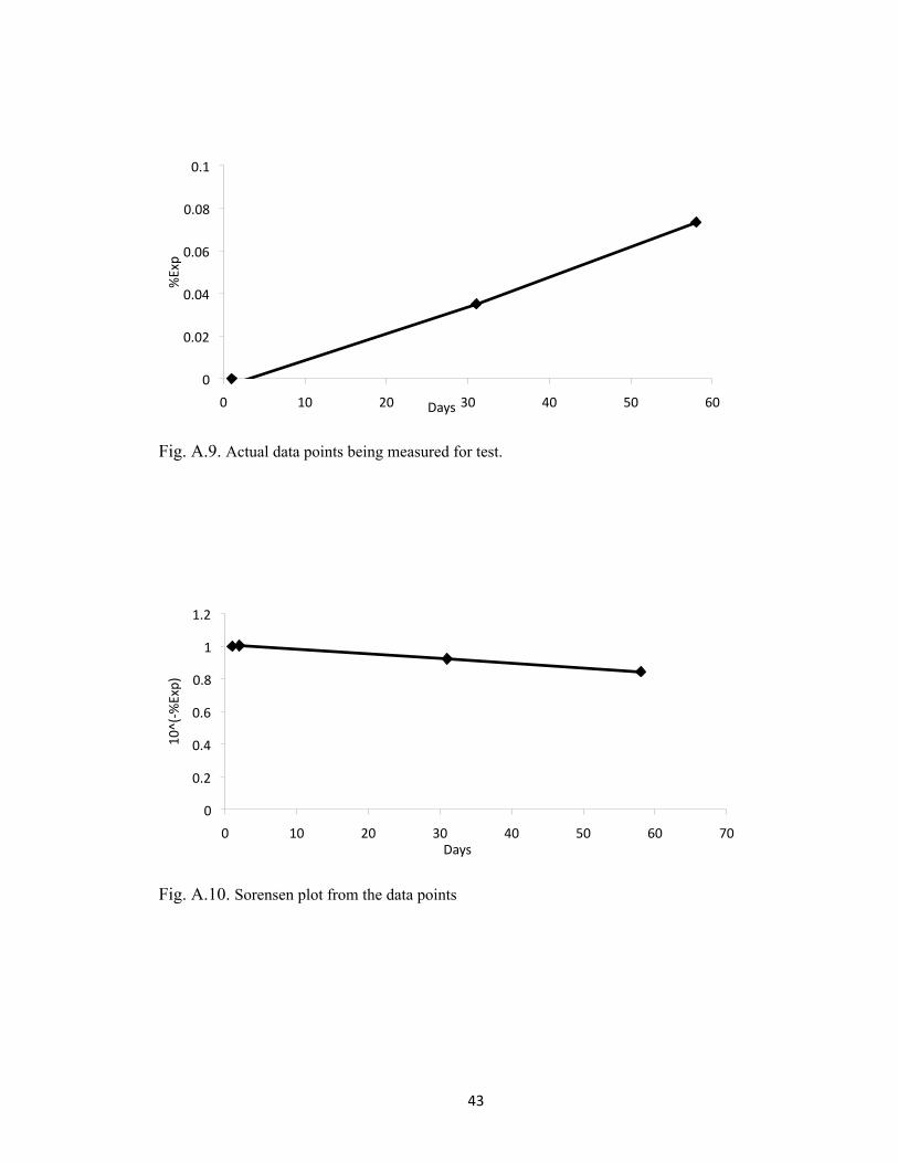
A.3 Example 3. Slow Accelerating Curve.

Data is collected and the Sorensen graph is made (fig. A.9 and A.10). This

continues until day 58 when the Sorensen turns slightly towards the X-axis. The

inflection point can now be calculated. First by creating a curve to fit the data (Fig.

A.11), second by plotting a Sorensen graph for the fitted curve (Fig. A.12). The

inflection point is then determined by extrapolating from the new Sorensen graph to the

X-axis. The extrapolated point from the Sorensen is 300 days. The inflection point

occurs after the last data point; therefore expansion must be interpolated from the actual

data or extending the fitted curve and using the expansion on day 300. Finding the

%expansion from the fitted curve on the day of the assumed inflection point gives a value

of 0.75. By using table 2.1 with a tc/tl ratio of 0.45 and an A value of 1.2 gives an

expected error of 15%. Finally, doubling the initial value for the final expansion gives

1.50. Table 2.1 says that this value is 15% over the typical value for a tc/tl ratio of 0.45.

Adjustments could be made to the final expansion which would lower the final expansion

to 1.28 %Exp. Actual is 1.16%Exp, 10.3% different. While this error may seem high it

allows one to complete the test at day 58 for a 619 day test.

43

Fig. A.9. Actual data points being measured for test.

Fig. A.10. Sorensen plot from the data points

0

0.02

0.04

0.06

0.08

0.1

0 10 20 30 40 50 60

%Exp

Days

0

0.2

0.4

0.6

0.8

1

1.2

0 10 20 30 40 50 60 70

10^(‐%

Exp)

Days

44

Fig. A.11. Fitted curve to actual data.

Fig. A.12. Extrapolating to find the assumed inflection point

0

0.02

0.04

0.06

0.08

0.1

0 10 20 30 40 50 60

%Exp

Days

0

0.2

0.4

0.6

0.8

1

1.2

0 50 100 150 200 250 300

10^(‐%

Exp)

Days

FiTedCurve

ExtrapolatedLine

VITA

Bret Robertson

Candidate for the Degree of

Master of Science Thesis: USING NUMERICAL TECHNIQUES TO ACCELERATE DELAYED

ETTRINGNITE FORMATION TEST METHODSTYPE FULL TITLE HERE IN ALL CAPS

Major Field: Civil Engineering Biographical: Bret Robertson was born in Ardmore, Oklahoma, on January 2, 1986. His

parents are Rob Robertson and Roberta Palmer. He has been married to Tara Robertson since July 28, 2007.

Education:

Completed the requirements for the Master of Science in Civil Engineering at Oklahoma State University, Stillwater, Oklahoma in May 2010.

Completed the requirements for the Bachelor of Science in Civil Engineering at Oklahoma State University, Stillwater, Oklahoma in December 2008. Graduated from Plainview High School in Ardmore, Oklahoma, in May 2004.

Professional Memberships: Member of Chi Epsilon, civil engineering honor society since 2009. Member of American Society of Civil Engineers since 2006. Member of American Concrete Institute since 2008. Member of American Institute of Steel Construction since 2007.

ADVISER’S APPROVAL: Tyler Ley

Name: John Bret Robertson Date of Degree: May, 2010* Institution: Oklahoma State University Location: Stillwater, Oklahoma Title of Study: USING NUMERICAL TECHNIQUES TO ACCELERATE DELAYED

ETTRINGNITE FORMATION TEST METHODS Pages in Study: 44 Candidate for the Degree of Master of Science

Major Field: Civil Engineering Scope and Method of Study: A numerical technique to be used to estimate the final results of tests with symmetric S-curves, specifically delayed ettringite formation expansion tests. Also Lab testing of cores with suspected DEF. Findings and Conclusions: Delayed ettringite formation (DEF) in concrete can cause significant damage to structures. Finding the severity of the DEF is beneficial. Currently to measure the potential DEF expansion, lab testing is required that could take up to 2 years to complete. This thesis presents two methods to shorten DEF expansion tests. Each method focuses on the following: fitting a curve to the data, assuming an inflection point, interpolating to the expansion of the found inflection point, and doubling the expansion found to obtain the final expansion. After considering each method, partial data from completed DEF expansion tests were used to compare final expansion results. Both methods accurately and consistently found final expansions while saving on average over a year of testing time. Making use of these methods would increase the time it takes to get information to the field about DEF expansions. Improving decision-making time concerning maintenance. DEF testing of cores from two projects was also performed. The Fu expansion test was used to measure the expansion of the cores over time.