using natural language processing to predict returns and

Using Natural Language Processing to Predict

Returns and Risk in the Oil Market

Nida Cakir Melek, Charles W. Calomiris, and Harry Mamaysky

September 2019

PRELIMIARY DRAFT:

NOT FOR QUOTATION WITHOUT AUTHORS’ PERMISSION

Authors appear here in alphabetical order by last name. Daliah Al-Shakhshir and Roya Arab

Loodaricheh provided excellent research assistance for this study. The views expressed herein

are solely those of the authors and do not necessarily reflect the views of the Federal Reserve

Bank of Kansas City or the Federal Reserve System.

1

1. Introduction

In this study, we ask several questions about the usefulness of natural language processing (NLP)

measures for forecasting outcomes in the oil market. Specifically, we investigate how the oil

market reacts to measures of news from energy-related articles that appear in Thomson Reuters

(TR) over the period 1998-2019. How can NLP be used alongside more traditional quantitative

measures to improve economic forecasts of returns and volatility in the oil market? How are the

forecasts of returns and volatility related? How do NLP measures facilitate the understanding of

time-varying risk premia in the oil market? Are NLP measures capturing risks that are priced in

the market, or non-priced aspects of news that forecast returns in ways that were not known to

market participants? Do these NLP measures also forecast oil production and inventories?

To address these questions, we first construct a baseline model of traditional forecasting

variables – which includes measures that have proven successful in prior empirical studies –

which we use to forecast, over 4-week and 8-week horizons, oil price returns, oil price volatility,

three large multinational oil and gas companies’ stock returns, oil production and oil

inventories.1 We then augment that baseline forecasting model with NLP measures that capture

news flow about events that are relevant for the oil market. These text-based time-series include

topic-specific frequency and sentiment of energy news, as well as its unusualness or “entropy”

(i.e., the frequency of occurrence of unusual strings of words). Topical context is defined by the

corpus of TR articles, based on an algorithm that identifies co-occurring lists of words. We

1 We also constructed, but do not report here, one-week and one-year ahead forecasting models. The explanatory

power of NLP variables is much weaker for the one-week horizon. There is evidence of forecasting power one-year

ahead, but a limited number of independent annual observations reduces the power of this analysis.

2

employ a network modularity approach for identifying topics, as in Calomiris and Mamaysky

(2019a).

In recent years, the modeling of commodity risk and returns has received increasing

attention, and several successful forecasting variables have been identified in the literature.

Contributions include Hong and Yogo (2012), Acharya et al. (2013), Gorton et al. (2013), and

Yang (2013). Given our goal – determining the incremental forecasting power of NLP measures

– we include in our baseline model a “kitchen sink” of forecasting variables, including some

variables not previously included in the above studies.2

Loughran et al. (2019) includes NLP measures in a forecasting model of oil price returns.

They construct a measure of sentiment – an oil tone index – and find it is useful for predicting oil

price returns at high frequency.3 Building on the empirical findings of Sinha (2016), Heston and

Sinha (2017), and Calomiris and Mamaysky (2019a, 2019b), which found that NLP measures are

useful for forecasting returns and risk over longer horizons, we consider forecasting horizons of

four weeks and eight weeks. Given that ours is a time-series rather than a panel analysis, our

sample size limits our ability to lengthen our forecasting horizon much beyond eight weeks.

We find that many of our NLP measures contain important explanatory power for oil

price returns, volatility, and oil company stock returns. This is true for both forecasting horizons,

but the NLP measures typically have more forecasting power at the 8-week horizon than at the 4-

week horizon. The NLP measures are not as useful for forecasting production or inventories over

2 In future drafts, we will also construct a parsimonious version of the baseline model based on a lasso model. 3 In related papers, while Kilian and Vega (2011) find no statistically significant impact of macroeconomic news on

oil prices, Elder et al. (2013) find a surprisingly strong correspondence between high frequency

jumps in oil prices and the arrival of new economic information.

3

those same horizons. Our future research will apply these measures to a decomposition of returns

that addresses the questions of whether the incremental forecasting power of NLP measures

captures priced or non-priced risk in oil returns, and whether NLP measures provides

incremental information about time variation in the oil market risk premium.

The remainder of our paper proceeds as follows. Section 2 presents our forecasting model

and describes our data sources and our methods for constructing the NLP measures included in

the model. Section 3 presents our results. Section 4 concludes.

2. Time-Series Forecasting Model

Our forecasting model includes a variety of variables that capture returns and risks in the

macroeconomy and the oil market, as well as text from TR news articles about the energy sector.

The raw data used to construct the variables used in our regressions come from Bloomberg, the

Energy Information Administration, the Wall Street Journal, and the Federal Reserve Board.

Table 1 presents definitions for all the variables used in the empirical analysis.

Our “kitchen sink” baseline model includes the following variables: oil price returns,

company stock returns, oil price volatility, the change in oil price volatility, the change in oil

production, the change in oil inventories, the VIX, the change in the VIX, the yield on the ten-

year Treasury note, the change in the trade-weighted value of the dollar, the market return on the

S&P 500, the futures basis (the ratio of the 3-month to 1-month price for crude oil futures), the

year-on-year growth rate of Baumeister and Hamilton (2019) world industrial production index,

and a linear time trend. We use lagged measures of these variables (defined precisely in Table 1)

as forecasters over 4-week and 8-week future horizons. Our model is estimated using

4

overlapping observations 4- and 8-week returns, which substantially increases degrees of

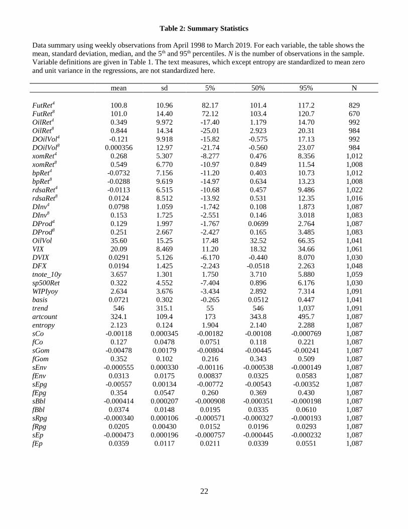
freedom for estimation.4 Table 2 reports summary statistics for all the variables used as either

dependent variables or forecasting variables in our model.

A note is in order on the timing of our weekly observations. Data on oil inventories and

production is released weekly on Wednesdays at 10:30am Eastern time. For some weeks

including holidays, releases are delayed by one or two days. For this reason, we use a weekly

return (spot or future) series that uses the closing price on Friday and goes to the Friday close of

the following week. We calculate j-week returns as the product of Friday to Friday single-week

returns. All right-hand side variables are released into the market prior to the Friday 2:30pm oil

futures market close.

Our augmented model includes all the variables in the baseline model, plus NLP

measures that capture the number of energy articles published in TR (artcount), each topic’s

relative frequency (f[Topic]), topic-specific sentiment (s[Topic]), and unusualness (entropy). We

will explain these series momentarily. All of these NLP measures are constructed as averages of

daily observations for the four-week period prior to the date of the forecast. All daily series are

word-weighted averages of the article-level measures within a given day, which for day t

includes articles from 2:30pm on day t-1 to 2:30pm on day t. For Mondays, we count articles

from 2:30pm to midnight on Friday, in addition to articles from 2:30pm on Sunday to 2:30pm on

Monday. The timing of the weekly series is to use data in a given week prior to the Friday

2:30pm oil futures market close.

4 It is well-known that the use of overlapping observations will downwardly bias standard errors and upwardly bias

R-squared. In results not reported here, we also ran our forecasting models using non-overlapping results and

obtained qualitatively similar results. In future drafts, we will make use of Monte Carlo methods to correct the

upward bias in our reported R-squareds.

5

2.1 Text Analytics

Our corpus for NLP analysis includes all the articles in Thomson Reuters (TR) that TR

regards as energy-related from 1998 to 2019.5 To perform topical analysis we compiled a list of

energy-related words, bigrams and trigrams (two- and three-word phrases respectively) from

several energy industry glossaries and other lists of energy words and phrases. This resulted in a

list of 387 tokens. We then construct a 387 × 387 co-occurrence matrix which measures the

cosine similarity between this initial list of tokens; the cosine similarity between tokens i and j is

given by 𝑤𝑖

⊤𝑤𝑗

‖𝑤𝑖‖‖𝑤𝑗‖ where 𝑤𝑖 is the vector measuring the number of times token i appears in all the

documents in our TR corpus. We then employ the Louvain algorithm (see Blondel et al. 2008)

to identify disjoint (i.e., non-overlapping) word groups that maximize the modularity (see

Newman and Girvan 2004) of the network represented by the word co-occurrence matrix. In this

step, we set the diagonal of the co-occurrence matrix to zero, which then yields eight topics from

the Louvain algorithm. The eighth topic contained only several tokens, so we reallocated these

tokens from the eighth topic to the other seven topics so as to maximize the resultant seven-topic

network’s modularity.

Once we had identified the initial set of seven topics, we calculated the average co-

occurrence of a large set of additional candidate energy related words, bigrams and trigrams with

the 387 initial energy words, bigrams and trigrams from the energy industry glossaries. We then

identified from the list of additional potential energy words those whose maximum topical co-

occurrence was very high relative to its average topical co-occurrence. For example, the

candidate token shell, which was not part of our original 387-token list, had an average cosine

5 The list of TR subject codes that we include in our analysis is shown in the appendix.

6

similarity with the existing tokens in topic 1 of 0.2076, whereas its average co-occurrence across

all seven topics was 0.0374. The resultant difference of 0.1702 was the second highest of all our

candidate tokens. We therefore included shell in our augmented token list. The intuition behind

this metric is that we wanted to exclude words that had high co-occurrence with all our topical

clusters because these tended to be generic words (such as said or though). However, words that

had a high co-occurrence with a single topic tended to be energy-related words or bi- or tri-

grams. Applying this process to a large set of candidate tokens yielded an additional 54 tokens,

which we then placed into one of the existing seven topical groups so as to maximize the

network modularity of the new, 441-token network.

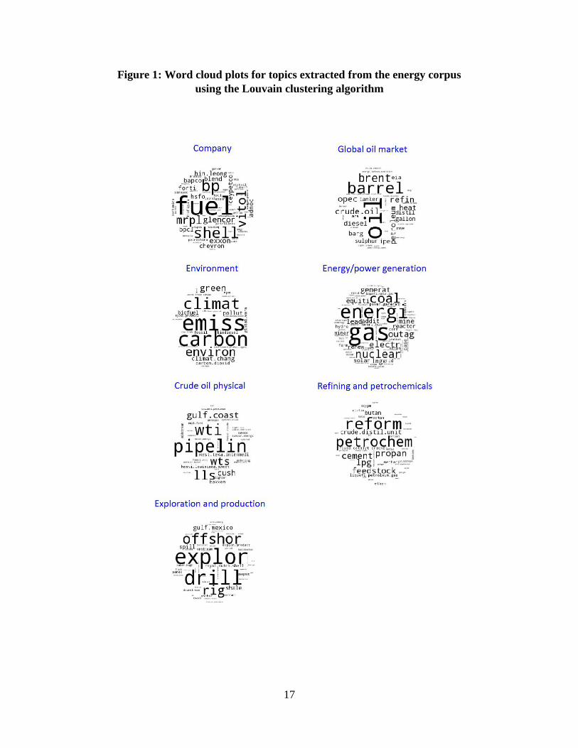
These seven non-overlapping word groups form the topic categories shown in Table 3.6

Figure 1 displays the word clouds for each of our seven topics. We label the topical categories

based on our interpretation of the common topical link defined by the words that appear in each

of these word clouds. Interestingly, the topics defined by the word clouds have readily

interpretable meaning and occur with sufficient frequency and variation over time to be useful in

our analysis. We label the topics as follows: company (Co), global oil market (Gom),

environment (Env), energy/power generation (Epg), crude oil physical (Bbl), refining and

petrochemicals (Rpc), and exploration and production (Ep). Allowing each topic’s frequency and

topic-specific sentiment to enter our model separately permits frequency and sentiment for the

various energy-related topics to differ in their directional effects and importance as forecasters.7

6 As a robustness check, we will verify that Latent Dirichlet Allocation yields a similar set of topics. Also, to

conserve space, we only show the most frequently occurring tokens in each topic. The full list of words and topic

allocations is available from the authors. 7 We also considered employing a more parsimonious specification of the augmented model that employs the first

and second principal components of our NLP measures. We found, however, that most of the NLP measures have

explanatory power in our forecasting models. This reflects the fact that the first principal component does not

capture a large percentage of the common variation contained in the individual NLP measures (in contrast, for

example, to the first principal component of the NLP measures in Calomiris and Mamaysky 2019a).

7

The seven topical category labels reflect our understanding of the meaning of the energy

words, which are corroborated by the sample headlines provided in Table 4. The table provides

examples of headlines for news articles with high topical scores in each of the seven categories,

for which we select two articles that have very high and very low sentiments respectively. The

table shows that headlines (for the most part) appear to be accurately classified using our topic

models, and further that the general tone of the headlines is well captured by our sentiment

scores.

The sentiment of words that appear in each TR article is defined using the Loughran-

McDonald sentiment dictionary. Sentiment is defined for each article as the different between the

number of positive sentiment and negative sentiment words, divided by the total number of

words (after stop words are removed and several other cleaning steps described in the appendix

are implemented) in the articles. Each article receives a topical weight based on the fraction of

all energy-related words appearing in that article that fall into a particular topic (recall that our

topics are disjoint, and so each word, bigram and trigram belongs to a single topic). For each

article, the article-topic weights sum to one. Articles are aggregated at the daily level using equal

weighting, and then averaged to obtain weekly measures of topical frequency and topic-specific

sentiment.

Unusualness is defined using the entropy concept introduced in Glasserman and

Mamaysky (2019) and Calomiris and Mamaysky (2019a). Specifically, we define an article’s

unusualness as the negative average log probability of all 4-grams appearing in that article, or

𝑎𝑟𝑡𝑖𝑐𝑙𝑒 𝑒𝑛𝑡𝑟𝑜𝑝𝑦 ≡ − ∑ 𝑝𝑖

𝑖∈4−𝑔𝑟𝑎𝑚𝑠𝑖𝑛 𝑡ℎ𝑒 𝑎𝑟𝑡𝑖𝑐𝑙𝑒

× log �̂�𝑖,

8

where 𝑝𝑖 is the fraction of all 4-grams represented by the 𝑖𝑡ℎ 4-gram, and �̂�𝑖 is the empirical

probability of the fourth word in the 4-gram conditional on the first three, estimated over a

training corpus using all articles from months 𝑡 − 27 to 𝑡 − 4. Further details are provided in the

appendix. We then average article entropy at the daily level, and then again at the weekly level.

A high unusualness score (or entropy) indicates that a week’s TR corpus articles contain a high-

proportion of four-grams that rarely appeared in prior weeks.

We plot the time series of each of our NLP measures in Figure 2. The time-series plots of

our NLP measures show that there is substantial variation over time in topical frequency, topic-

specific sentiment, and unusualness measures.

3. Empirical Findings

We consider eight dependent variables. For each variable, we construct baseline and augmented

forecasting models, where the latter include all the NLP measures. We consider two measures of

oil price returns as dependent variables. The first, (𝑃𝑡+𝑗

𝑃𝑡− 1), measures percent spot price

changes over a j week period, where j = 4, 8, using the front-month futures contract as the

measure of spot price, as in Kilian and Vega (2011) and Loughran et al. (2019). While a useful

test of model’s ability to capture the dynamics of oil prices, spot price changes do not represent

an investable return because they ignore storage and transportation costs. To capture an

investable oil price series, we construct the realized returns from investing each week in the

front-month oil future. On weeks that the front month future expires, we measure returns using

an investment in the second month oil future (which will become the front month at the end of

the week). We construct j-week returns as the product of the past j weeks’ one-week returns, as

9

in Acharya et al. (2013), Gorton et al. (2013), Hong and Yogo (2012), and Yang (2013). This

second measure captures the returns to a specific speculative investment strategy, and thus

reflects changes in spot prices, the realization of risk premia and changes in risk premia over

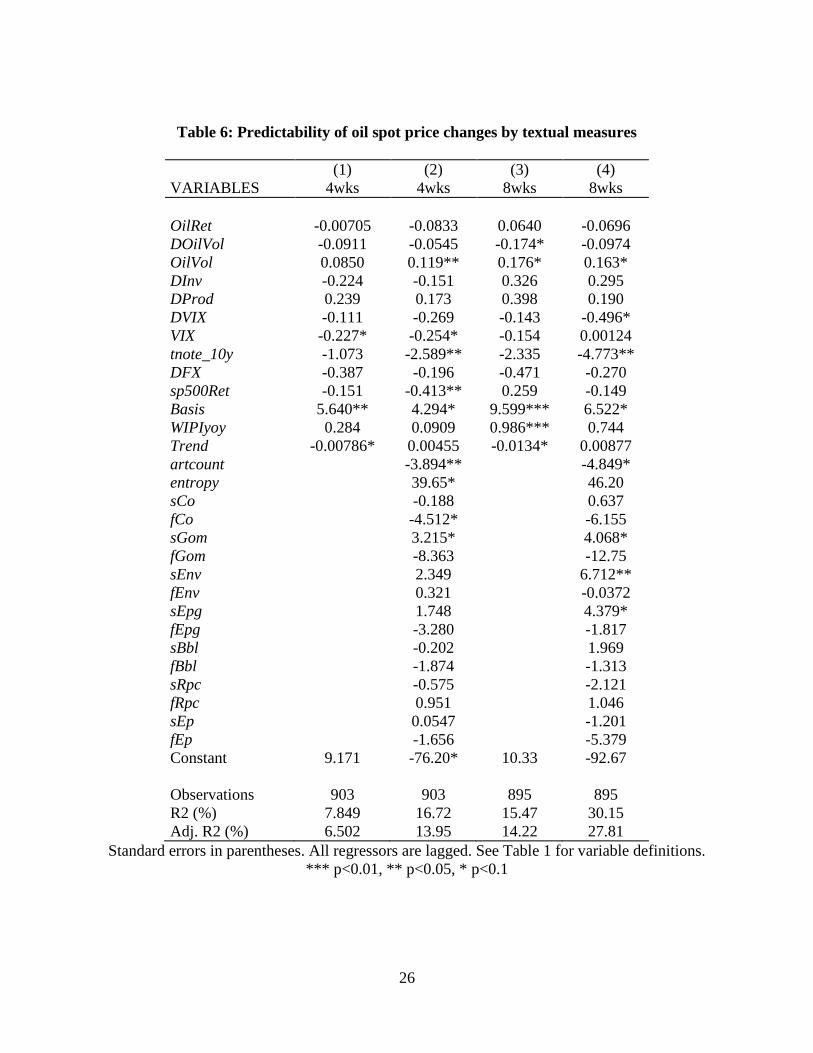
time. We report our findings for our forecasting models of these two variables in Tables 5 and 6.

We forecast oil price volatility, which is measured using the realized oil price volatility

index from Bloomberg. These results are reported in Table 7. We model the stock returns of

three major oil and gas companies (BP, Shell, and Exxon) in Tables 8, 9, and 10, respectively.

Tables 11 and 12 report results for forecasting oil inventories and production.

Table 13 summarizes our findings with respect to statistically significant forecasting by

our NLP measures for each of the eight dependent variables.8 Several overarching patterns are

visible in Tables 5-13, and we focus our discussion on those observations.

First, NLP measures clearly add to the explanatory power of futures returns, spot returns,

volatility, the three oil and gas companies’ stock returns, and oil inventories, and there is weak

evidence that they are useful for forecasting oil production. For all the variables except

production, the forecasting improvement from including NLP measures is visible both in the

substantial increases in adjusted R-squared that result from the inclusion of the NLP variables,

and the statistical significance of many of the NLP coefficients.

In the case of oil futures returns, eight of the NLP measures are statistically significant

either in the 4-week or 8-week regressions, and adjusted R-squared is much higher in the

augmented models than in the baseline models (at the 8-week horizon, it rises from 24.5 percent

8 We refrain from discussing the performance of the baseline models in detail, although we will comment on some

specific baseline variables in the course of our discussion of the NLP measures.

10

to 42.8 percent when the NLP measures are included). Six of the NLP measures are significant in

one or both of the augmented spot return models, and adjusted R-squared improves dramatically

in the augmented models (at the 8-week horizon, it rises from 14.2 percent to 27.8 percent).

In the volatility regressions, four NLP measures prove significant, and adjusted R-

squared increases are more modest, reflecting the fact that volatility is highly forecastable on the

basis of its own level, change, oil returns, and the VIX.

For oil companies’ returns, many NLP measures prove significant in one or both of the

augmented regressions (five for Exxon, eight for BP, and six for Shell), and adjusted R-squareds

rise dramatically (at the 8-week horizon, adjusted R-squareds in the augmented model rise in

comparison with the baseline model from 8.7 to 15.6, from 6.2 to 22.9 and from 6.2 to 22.0

percent, respectively, for the three companies’ stock returns).

For oil inventories, four NLP measures are individually significant in one or both of the

augmented models, and adjusted R-squareds improve dramatically as the result of the inclusion

of NLP variables (at the 8-week horizon, rising from 10.6 percent in the baseline model to 25.5

percent in the augmented model).

In the case of oil production, none of the NLP coefficients is statistically significant, but

there is some improvement in adjusted R-squared from their inclusion, especially at the 8-week

horizon, where adjusted R-squared rises from 10.6 percent in the baseline model to 13.6 percent

in the augmented model.

Second, when NLP results are significant for both the 4-week and 8-week horizons, their

coefficients always have the same sign, and it is noteworthy that the NLP coefficients’

magnitudes (in absolute value), their statistical significance, and their effect on adjusted R-

11

squared all tend to be larger at the 8-week horizon than at the 4-week horizon. Whatever the

augmented models are capturing is a persistent influence that remains as important, or grows in

importance, from the fourth to the eighth week horizon in the future (coefficient values

sometimes more than double, indicating greater effects for the second month than the first).

Third, there is remarkable consistency in the NLP variables effects on the five returns

measures (oil future returns, oil spot returns, and the three companies’ stock returns). For those

five dependent variables, when an NLP measure enters significantly for more than one of those

dependent variables, it always enters with the same sign. As Table 13 shows, there is substantial

overlap of each NLP measure for forecasting significantly across the five returns measures. Five

of the six NLP measures that are significant in one or both of the augmented models of spot

returns are also significant in the augmented model of futures returns. There is also substantial

overlap in which NLP variables enter the oil returns and the companies’ stock returns. The

following NLP measures appear as significant predictors in at least three of the five returns

regressions: artcount, entropy, sCo, fGom, sEnv, sEpg, sEp, and fEP. Additionally, fCo appears

in two of the five.

Fourth, there is also remarkable consistency in the opposite sign of significant NLP

measures that both affect returns measures (one or more of the five returns variables) and

volatility. When artcount or fGom enter into any returns measures, they have a negative sign

(more energy news is bad news for returns), but they enter positively for volatility. When

entropy or sGom enter in returns measures, they have a positive sign, but their signs are negative

for volatility.

This opposite effect on returns measures and volatility is also visible for some of the

significant forecasting variables that are included in the baseline models. VIX is positive for

12

volatility but negative for oil futures and oil spot returns. WIPIyoy is positive for oil futures and

spot returns and for the stock returns of Exxon and Shell, but it is negative for volatility. OilVol

is negative for itself but positive for several returns variables. However, not all the baseline

forecasters have opposite effects on returns measures and volatility. VIX is positive for Shell

returns and volatility, and basis is positive for both volatility and oil spot returns (but negative

for BP returns).9

The tendency for our NLP and baseline variables to have opposite signs in predicting

returns and volatility variables suggests that the news contained in these variables is not priced

risk. Generally, when there is a positive risk premium, information about changes in risk that are

priced in the market should have the same sign for (expected) returns as for volatility. Calomiris

and Mamaysky’s (2019a) study of stock returns and risk, for example, interpreted the opposite

signs of NLP measures for forecasting returns and risk as indicating that the news contained in

the NLP measures was not priced risk. That is, it appears that the information was news that was

not immediately known by the market, and only later affected returns as it became known (i.e., it

mattered for returns but not for expected returns at the dates the articles appeared). This same

interpretation could be applied to some of the baseline forecasters, too. For example, WIPIyoy

enters positively as a predictor of returns, but we expect that it captures good news about the

expansion of global oil demand, not risk.

However, an alternative interpretation is also possible. It may be that oil markets contain

a negative volatility risk premium. Indeed, Baumeister and Kilian (2017) suggest that the oil risk

premium has changed from slightly negative on average prior to 2004 to negative post-2004. If

9 In theory, and consistent with prior empirical findings, we expect the univariate relationship between basis and oil

futures returns to be negative. In univariate regression results, we did find a negative coefficient on basis, but in the

multivariate models reported in Table 5, basis is consistently insignificantly different from zero.

13

the risk premium is negative, then information about risk that is priced in the market at the time

the articles appear may have opposite forecasting implications for volatility and returns. In a

future draft, we will investigate this question formally.

Fifth, when topic-specific sentiment measures enter significantly they tend to have

positive effects on returns. That is consistently true for the effects of sCo, sGom, sEnv, sEpg on

the five returns variables. However, two of the topic-specific sentiment measures have negative

effects on returns. sEp is negative significant for all three companies’ stock returns, and sRpc is

negative significant for oil futures returns. Calomiris and Mamaysky (2019a) also found that

topic-specific sentiment can vary in sign for forecasting stock returns depending on the topic.

Indeed, that is one of the reasons to distinguish sentiment according to its topical context, as we

do in our augmented model. One interpretation of the negative signs for sEp and sRpc is that

these two variables measure sentiment that is more related to the supply of oil and refined

products than to their demand. Positive sentiment about expansion of oil and refined products

supply may be negative news for oil prices, and therefore, negative news for oil and gas

companies’ returns. The fact that the two sentiment measures do not have significant and

consistent signs across companies’ returns models and oil returns models, however, does not

provide strong empirical support for this conjecture.

Finally, turning to the augmented model of oil inventories in Table 11, some results are

interesting. OilVol has a positive effect in the baseline models, as inventory theory would suggest

(higher inventories reduces the exposure to price change), but it is not robustly significant in the

augmented models. We note, however, that entropy, which enters negatively in the volatility

regressions, also enters negatively in the inventory regressions, so it may be that some aspects of

forecasted increases in volatility are associated with increased inventories. sEp negatively

14

predicts inventories, which is consistent with its possible role as a predictor of expanded supply

(if prices are expected to fall, then there is less need to protect against potential price increases).

4. Conclusions

NLP measures of energy markets provide substantial incremental explanatory power for

forecasting oil price returns and volatility, and oil company stock returns. They are also useful

for forecasting oil inventories, but not very useful for forecasting oil production. The explanatory

power of NLP measures is visible for most of the 16 NLP measures we include in our model,

which capture topical frequencies, topic-specific sentiment, and unusualness of text flow in the

TR energy corpus. Results are similar for the 4-week and 8-week horizons, although explanatory

power is greater for the 8-week horizon.

In future drafts, we will focus on two additional questions. First, we will investigate the

extent to which the NLP measures’ ability to forecast returns reflect priced risks vs. unpriced

news that is contained in the NLP measures but that was not known at the time the articles from

which those measures were constructed were written. Second, we will ask whether NLP

measures are useful for improving the predictions of time-varying risk premia in oil markets.

Appendix

[TO BE COMPLETED.]

15

References

Acharya, Viral, Lars A. Lochstoer, and Tarun Ramadorai. 2013. “Limits to Arbitrage and

Hedging: Evidence from Commodity Markets,” Journal of Financial Economics 109, 441-

465.

Baumeister, Christiane, and James Hamilton. 2019. “Structural Interpretation of Vector

Autoregressions with Incomplete Identification: Revisiting the Role of Oil Supply and

Demand Shocks,” American Economic Review 109, 1873-1910.

Baumeister, Christiane, and Lutz Kilian. 2017. “A General Approach to Recovering Market

Expectations from Futures Prices with an Application to Crude Oil,” Working Paper.

Blondel, V., J.-L. Guillaume, R. Lambiotte, and E. Lefebvre, 2008, “Fast unfolding of

communities in large networks,” Journal of Statistical Mechanics, 10, 10008.

Calomiris, Charles W., and Harry Mamaysky. 2019a. “How News and Its Context Drive Risk

and Returns Around the World,” Journal of Financial Economics 133, 299-336.

Calomiris, Charles W., and Harry Mamaysky. 2019b. “Monetary Policy and Exchange Rate

Returns: Time-Varying Risk Regimes.” NBER Working Paper No. 25714, April.

Elder, John, Hong Miao, and Sanjay Ramchander. 2013. “Jumps in Oil Prices: The Role of

Economic News,” The Energy Journal 34, 217-237.

Glasserman, Paul, and Harry Mamaysky. 2019. “Does Unusual News Forecast Market Stress?”

Journal of Financial and Quantitative Analysis, forthcoming.

Gorton, Gary, Fumio Hayashi, and K. Geert Houwenhorst. 2013. “The Fundamentals of

Commodity Futures Returns,” Review of Finance 17, 35-105.

Heston, S., and N.R. Sinha. 2017. News vs. Sentiment: Predicting Stock Returns from News

Stories,” Financial Analysts Journal 73, 67-83.

Hong, Harrison, and Motohiro Yogo. 2012. “What Does Futures Market Interest Tell Us About

the Macroeconomy and Asset Prices?” Journal of Financial Economics 105, 173-490.

Kilian, Lutz, and Clara Vega. 2011. “Do Energy Prices Respond to U.S. Macroeconomic News?

A Test of the Hypothesis of Predetermined Energy Prices,” Review of Economics and

Statistics 93, 660-671.

Loughran, Tim, Bill McDonald, and Ioannis Pragidis. 2019. “Assimilation of Oil News Into

Prices,” International Review of Financial Analysis 63, 105-118.

Newman, M.E.J. and M. Girvan, 2004, “Finding and evaluating community structure in

networks,” Physical Review E, 69, 026113.

16

Sinha, N.R. 2016. “Underreaction to News in the U.S. Stock Market,” Quarterly Journal of

Finance 6, 1-46.

Yang, Fan. 2013. “Investment Shocks and the Commodity Basis Spread,” Journal of Financial

Economics 110, 164-184.

17

Figure 1: Word cloud plots for topics extracted from the energy corpus

using the Louvain clustering algorithm

18

Figure 2: NLP measures over time

21

Table 1: Data definitions summary.

“Topic” below is one of company (Co), global oil market (Gom), environment (Env), energy/power

generation (Epg), crude oil physical (Bbl), refining and petrochemicals (Rpg), or exploration and

production (Ep). The forecasting horizon, h, is one of 4 or 8 weeks.

Data definitions summary

Variable Definition

FutReth WTI front-month futures cumulative weekly returns (in %) starting in week t through

week t+h

DSpoth Percent change in the WTI spot price from week t to t+h

DOilVolh Level difference in the rolling 30-day realized volatility of WTI physical futures 1-month

nearby contract between weeks t+h and t

xomReth Exxon Mobil stock returns (in %) from week t to week t+h

bpReth British Petrol stock returns from week t to week t+h

rdsaReth Royal Dutch Shell class A stock returns from week t to week t+h

DInvh Percent change in U.S. crude inventories including SPR (EOP, mil. bbl) from week t to

week t+h

DProdh Average weekly percent change in U.S. crude oil field production (mil. bbl/day) from

week t to week t+h

OilVol Rolling 30-day realized volatility of WTI physical futures 1-month nearby contract

VIX CBOE market volatility index

DVIX Level difference in the CBOE market volatility index relative to 4 weeks ago

DFX Percent change in the nominal broad dollar index - goods only (Jan 1997 = 100)

relative to 4 weeks ago

tnote_10y 10-year treasury note yield at constant maturity (EOP, % p.a.)

sp500Ret Standard and Poor’s 500 stock returns relative to 4 weeks ago

basis WTI physical 3-month to 1-month basis (when positive curve is upward sloping,

capturing contango)

WIPIyoy Year-over-year growth rate of Baumeister and Hamilton’s (2019) monthly World

Industrial Production Index

trend Weekly linear time trend

f[Topic] Average frequency of articles over the previous 4 weeks in Topic

s[Topic] Average sentiment over the previous 4 weeks due to Topic

artcount Average number of articles in the energy corpus over the past 4 weeks

entropy Average measure of article unusualness over the past 4 weeks

22

Table 2: Summary Statistics

Data summary using weekly observations from April 1998 to March 2019. For each variable, the table shows the

mean, standard deviation, median, and the 5th and 95th percentiles. N is the number of observations in the sample.

Variable definitions are given in Table 1. The text measures, which except entropy are standardized to mean zero

and unit variance in the regressions, are not standardized here.

mean sd 5% 50% 95% N

FutRet4 100.8 10.96 82.17 101.4 117.2 829

FutRet8 101.0 14.40 72.12 103.4 120.7 670

OilRet4 0.349 9.972 -17.40 1.179 14.70 992

OilRet8 0.844 14.34 -25.01 2.923 20.31 984

DOilVol4 -0.121 9.918 -15.82 -0.575 17.13 992

DOilVol8 0.000356 12.97 -21.74 -0.560 23.07 984

xomRet4 0.268 5.307 -8.277 0.476 8.356 1,012

xomRet8 0.549 6.770 -10.97 0.849 11.54 1,008

bpRet4 -0.0732 7.156 -11.20 0.403 10.73 1,012

bpRet8 -0.0288 9.619 -14.97 0.634 13.23 1,008

rdsaRet4 -0.0113 6.515 -10.68 0.457 9.486 1,022

rdsaRet8 0.0124 8.512 -13.92 0.531 12.35 1,016

DInv4 0.0798 1.059 -1.742 0.108 1.873 1,087

DInv8 0.153 1.725 -2.551 0.146 3.018 1,083

DProd4 0.129 1.997 -1.767 0.0699 2.764 1,087

DProd8 0.251 2.667 -2.427 0.165 3.485 1,083

OilVol 35.60 15.25 17.48 32.52 66.35 1,041

VIX 20.09 8.469 11.20 18.32 34.66 1,061

DVIX 0.0291 5.126 -6.170 -0.440 8.070 1,030

DFX 0.0194 1.425 -2.243 -0.0518 2.263 1,048

tnote_10y 3.657 1.301 1.750 3.710 5.880 1,059

sp500Ret 0.322 4.552 -7.404 0.896 6.176 1,030

WIPIyoy 2.634 3.676 -3.434 2.892 7.314 1,091

basis 0.0721 0.302 -0.265 0.0512 0.447 1,041

trend 546 315.1 55 546 1,037 1,091

artcount 324.1 109.4 173 343.8 495.7 1,087

entropy 2.123 0.124 1.904 2.140 2.288 1,087

sCo -0.00118 0.000345 -0.00182 -0.00108 -0.000769 1,087

fCo 0.127 0.0478 0.0751 0.118 0.221 1,087

sGom -0.00478 0.00179 -0.00804 -0.00445 -0.00241 1,087

fGom 0.352 0.102 0.216 0.343 0.509 1,087

sEnv -0.000555 0.000330 -0.00116 -0.000538 -0.000149 1,087

fEnv 0.0313 0.0175 0.00837 0.0325 0.0583 1,087

sEpg -0.00557 0.00134 -0.00772 -0.00543 -0.00352 1,087

fEpg 0.354 0.0547 0.260 0.369 0.430 1,087

sBbl -0.000414 0.000207 -0.000908 -0.000351 -0.000198 1,087

fBbl 0.0374 0.0148 0.0195 0.0335 0.0610 1,087

sRpg -0.000340 0.000106 -0.000571 -0.000327 -0.000193 1,087

fRpg 0.0205 0.00430 0.0152 0.0196 0.0293 1,087

sEp -0.000473 0.000196 -0.000757 -0.000445 -0.000232 1,087

fEp 0.0359 0.0117 0.0211 0.0339 0.0551 1,087

23

Table 3: Topic word lists.

This table shows the top 20 tokens by frequency in each topical group.

Topic WordList

global oil market (gom) oil (4,136,780), barrel (1,226,580), brent (526,719), refin (411,872), crude.oil

(409,276), opec (394,754), petroleum (293,525), heat (291,997), diesel (276,319),

barg (194,018), ipe (175,841), distil (167,863), tanker (142,160), sulphur

(140,039), gallon (136,243), eia (127,622), nwe (70,962), ara (62,293),

energi.inform.administr (55,927), bunker (47,736)

energy/power generation

(epg)

gas (2,082,748), energi (1,385,165), coal (510,535), outag (409,463), nuclear

(381,919), electr (326,305), generat (225,899), equiti (184,324), mine (178,868),

lead (165,664), lng (162,184), addit (142,116), reactor (125,164), renew

(120,903), solar (101,509), case (91,068), miner (90,722), grid (79,484), hydro

(69,220), power.generat (53,787)

company (co) fuel (1,483,081), bp (369,851), shell (369,655), vitol (237,656), mrpl (220,506),

hsfo (158,878), glencor (144,515), exxon (136,651), mop (121,139), hin.leong

(113,240), ceypetco (102,883), chevron (96,915), bpcl (95,996), petrochina

(93,576), bapco (92,908), essar (90,448), blend (88,597), pertamina (84,403),

trafigura (83,198), forti (81,329)

crude oil physical (bbl) pipelin (409,704), wti (321,512), lls (169,911), wts (117,949), gulf.coast (68,858),

cush (53,943), west.texa.intermedi (35,191), bakken (31,987),

heavi.louisiana.sweet (22,581), enbridg (18,568), midstream (17,634), permian

(13,138), sunoco (12,958), heavi.crude (9,681), lighter (8,541), heavi.oil (8,333),

eagl.ford (8,053), suncor.energi (7,419), occident.petroleum (5,411),

permian.basin (5,366)

Environment (env) emiss (189,038), carbon (176,792), climat (105,968), environ (61,429), green

(49,666), climat.chang (46,992), pollut (45,532), biofuel (32,514), carbon.dioxid

(24,075), epa (22,403), biodiesel (19,407), global.warm (19,067), fossil (18,012),

valv (10,182), kyoto.protocol (9,235), environment.protect.agenc (8,036), methan

(7,179), emiss.trade.scheme (6,951), alki (6,204), air.pollut (4,723)

exploration & production (ep) explor (148,206), drill (137,958), offshor (123,543), rig (94,639), shale (58,500),

gulf.mexico (52,649), spill (46,891), royal.dutch.shell (37,685), onshor (28,528),

pemex (26,894), explor.product (23,701), upstream (23,476), downstream

(21,409), baker.hugh (17,968), deepwat (17,860), extract (17,115), halliburton

(11,329), texaco (10,093), frack (9,383), transocean (9,373)

refining & petrochemicals

(rpc)

reform (110,766), petrochem (88,297), cement (22,637), lpg (20,345), feedstock

(18,355), propan (18,259), crude.distil.unit (12,005), netback (7,888), butan

(7,407), liquefi.petroleum.gas (6,682), octan (6,045), fluid.catalyt.cracker (5,842),

ethan (5,737), visbreak (5,079), olefin (4,370), oxygen (3,418), benzen (2,738),

tertiari (2,081), polym (2,075), urea (1,830)

24

Table 4: Sample sentences with high and low sentiment for each topic category

Topic Sentiment Headline

company (co) 0.0076 Glencore holds talks with Chinalco over Rio Tinto tie-up –Bloomberg

company (co) 0.0098 UPDATE 1-Asia Jet Fuel-China Aviation issues Q4 tender

company (co) (0.0716) RPT-UPDATE 3-U.S. board issues urgent call for BP safety panel

company (co) (0.0488) BP appeals Russian court ruling on office search

global oil market (gom) 0.0309 Algeria says oil producers mulling cuts beyound March

global oil market (gom) 0.0280 Oil price not dramatic for German economy-Mueller

global oil market (gom) (0.0730) ANALYSIS-Chavez referendum defeat poses possible oil risk

global oil market (gom) (0.0714) U.S. crude falls over $2, Brent extends losses

Environment (env) 0.0179 TABLE-EU releases preliminary 2006 C02 emissions data

Environment (env) 0.0318 UPDATE 1-Obama sees climate deal in Copenhagen -White House

Environment (env) (0.0726) German court document names 150 CO2 tax fraud suspects

Environment (env) (0.0647) EU's big 3 van makers put brakes on CO2 curbs

energy/power generation (epg) 0.0192 Germany's big four utilities to boost transparency

energy/power generation (epg) 0.0168 RITV-Cheaper Solar Power in Pipeline: Areva - New show available

energy/power generation (epg) (0.0783) Moody's cuts Enron, warns of ""low"" recovery rates

energy/power generation (epg) (0.0894) NATGAS PIPELINE CRITICAL NOTICE: Southern Natural Gas Revised

Fairburn Force Majeure Notice

crude oil physical (bbl) 0.0270 U.S. cash crude price slide linked to futures fall

crude oil physical (bbl) 0.0229 November U.S. cash crudes trade quietly, WTS firm

crude oil physical (bbl) (0.0500) U.S. Cash Crude - WTI/Midland firms on cold supply concerns

crude oil physical (bbl) (0.0411) U.S. Cash Crudes - LLS off as Syncrude concerns fade

refining & petrochemicals (rpc) 0.0169 Union Carbide <UK.N> seeks E.Europe petchem deals

refining & petrochemicals (rpc) 0.0432 India's Reliance, GAIL sign petrochemicals deal

refining & petrochemicals (rpc) (0.0765) TEXT-S&P cuts LyondellBasell Industries rating to 'B-'

refining & petrochemicals (rpc) (0.1075) UPDATE 1-Brazil's political crisis halts labor reform bill

exploration & production (ep) 0.0556 Mexico says implementing measures to boost Pemex finances

exploration & production (ep) 0.0667 BRIEF-SSE in offshore wind pact with Siemens, Subsea 7, Atkins

exploration & production (ep) (0.0718) UPDTAE 1-Goldman removes Halliburton from conviction buy list

exploration & production (ep) (0.0702) BRIEF-Halliburton says in case of deal termination it would have to pay

$1.5 bln as fees to Baker Hughes

25

Table 5: Predictability of oil futures returns by textual measures

(1) (2) (3) (4)

VARIABLES 4wks 4wks 8wks 8wks

FutRet 0.156* 0.0719 0.187* 0.0737

DOilVol -0.162 -0.150 -0.0825 -0.0633

OilVol 0.179** 0.246** 0.164 0.216

DInv -0.979 -0.900 -1.796* -1.029

DProd 0.435** 0.354* 0.544** 0.287

DVIX -0.0536 -0.216 0.198 -0.219

VIX -0.363** -0.530*** -0.409** -0.347

tnote_10y -1.512 -2.933* -3.953** -7.027***

DFX -0.242 0.00926 0.313 0.986

sp500Ret -0.158 -0.508* 0.468 -0.0828

Basis 1.625 -0.111 6.445 4.943

WIPIyoy 0.468* 0.238 1.574*** 1.633***

Trend -0.00862 -0.00595 -0.0193** 0.00618

artcount -3.167 -6.049*

entropy 30.77 63.77*

sCo 0.450 2.460

fCo -6.252* -11.53**

sGom 3.247 3.106

fGom -12.46 -26.26**

sEnv 3.208 7.715**

fEnv 2.136 4.099

sEpg 1.404 6.456***

fEpg -7.235* -14.04***

sBbl 0.249 2.349

fBbl -2.317 -2.225

sRpc -1.007 -3.991**

fRpc -0.234 -1.523

sEp 0.256 0.521

fEp -0.856 -4.456

Constant 94.93*** 43.84 104.1*** -25.27

Observations 634 634 500 500

R2 (%) 13.77 21.26 26.50 46.13

Adj. R2 (%) 11.97 17.48 24.54 42.80

Standard errors in parentheses. All regressors are lagged. See Table 1 for variable definitions.

*** p<0.01, ** p<0.05, * p<0.1

26

Table 6: Predictability of oil spot price changes by textual measures

(1) (2) (3) (4)


OilRet -0.00705 -0.0833 0.0640 -0.0696

DOilVol -0.0911 -0.0545 -0.174* -0.0974

OilVol 0.0850 0.119** 0.176* 0.163*

DInv -0.224 -0.151 0.326 0.295

DProd 0.239 0.173 0.398 0.190

DVIX -0.111 -0.269 -0.143 -0.496*

VIX -0.227* -0.254* -0.154 0.00124

tnote_10y -1.073 -2.589** -2.335 -4.773**

DFX -0.387 -0.196 -0.471 -0.270

sp500Ret -0.151 -0.413** 0.259 -0.149

Basis 5.640** 4.294* 9.599*** 6.522*

WIPIyoy 0.284 0.0909 0.986*** 0.744

Trend -0.00786* 0.00455 -0.0134* 0.00877

artcount -3.894** -4.849*

entropy 39.65* 46.20

sCo -0.188 0.637

fCo -4.512* -6.155

sGom 3.215* 4.068*

fGom -8.363 -12.75

sEnv 2.349 6.712**

fEnv 0.321 -0.0372

sEpg 1.748 4.379*

fEpg -3.280 -1.817

sBbl -0.202 1.969

fBbl -1.874 -1.313

sRpc -0.575 -2.121

fRpc 0.951 1.046

sEp 0.0547 -1.201

fEp -1.656 -5.379

Constant 9.171 -76.20* 10.33 -92.67


R2 (%) 7.849 16.72 15.47 30.15

Adj. R2 (%) 6.502 13.95 14.22 27.81


*** p<0.01, ** p<0.05, * p<0.1

27

Table 7: Predictability of oil volatility by textual measures

(1) (2) (3) (4)


DOilVol -0.0527 -0.0505 -0.163** -0.174***

OilVol -0.386*** -0.490*** -0.573*** -0.717***

OilRet -0.290*** -0.272*** -0.323*** -0.257***

DInv 0.108 0.0539 0.369 0.460

DProd -0.211 -0.271 -0.193 -0.216

DVIX -0.125 -0.179 -0.187 -0.210

VIX 0.247*** 0.415*** 0.389*** 0.622***

tnote_10y 1.310* 0.496 3.072*** 2.992**

DFX 0.266 0.157 0.912 0.807*

sp500Ret -0.114 -0.0354 -0.0850 0.125

Basis 3.880** 4.204** -0.168 1.249

WIPIyoy -0.164 -0.0885 -0.465* -0.209

Trend 0.00193 0.00334 0.00836 0.00451

artcount 2.925** 3.129

entropy -48.99** -97.58***

sCo 0.171 0.810

fCo -0.199 0.979

sGom -1.462 -4.169**

fGom 8.347 12.50*

sEnv 0.170 0.478

fEnv -1.579 -0.124

sEpg 1.001 -0.194

fEpg 2.889 3.277

sBbl 0.682 1.050

fBbl 0.362 0.870

sRpc -0.330 0.0883

fRpc 0.0852 -0.726

sEp 0.854 1.807

fEp 0.149 2.633

Constant 3.110 109.4** -2.170 207.0***


R2 (%) 28.21 35.30 37.79 46.62

Adj. R2 (%) 27.16 33.15 36.87 44.83

Standard errors in parentheses. All regressors are lagged. See Table 1 for variable defnitions.

*** p<0.01, ** p<0.05, * p<0.1

28

Table 8: Predictability of Exxon stock returns by textual measures

(1) (2) (3) (4)


xomRet -0.167*** -0.167*** -0.260*** -0.249***

DOilVol -0.0138 0.000906 -0.0134 0.0151

OilVol 0.0193 0.0119 0.0578 0.0522

OilRet 0.0336 0.0286 0.0422 0.0281

DInv 0.398 0.407 0.557 0.552

DProd 0.162 0.134 0.0969 0.0810

DVIX -0.00730 -0.0729 0.0513 -0.0926

VIX 0.0327 0.104* 0.0558 0.140

tnote_10y -0.785* -1.505*** -1.411** -1.978**

DFX 0.125 0.237 0.208 0.303

sp500Ret -0.0398 -0.113 0.0930 -0.0830

Basis -0.0883 -0.434 -0.956 -1.899

WIPIyoy 0.242** 0.229** 0.446** 0.288

Trend -0.00316 0.000265 -0.00545* -0.00232

Artcount -0.597 -0.532

Entropy 16.49 23.02

sCo 0.771 1.769**

fCo -0.287 -0.322

sGom -0.0393 -0.204

fGom -3.170 -6.453*

sEnv 0.190 0.971

fEnv -0.773 -1.202

sEpg 1.520* 2.901**

fEpg 0.208 -0.204

sBbl 0.240 0.311

fBbl 0.129 -0.258

sRpc 0.310 0.0765

fRpc -0.172 -0.622

sEp -1.197* -1.904**

fEp -2.362*** -2.814**

Constant 2.946 -32.39 4.560 -44.94


R2 (%) 8.457 13.18 10.15 18.41

Adj. R2 (%) 7.031 10.23 8.741 15.61


*** p<0.01, ** p<0.05, * p<0.1

29

Table 9: Predictability of BP stock returns by textual measures

(1) (2) (3) (4)


bpRet -0.163** -0.170*** -0.258*** -0.270***

DOilVol -0.0177 0.0193 -0.0385 0.0370

OilVol 0.0463 0.0408 0.0969* 0.0801

OilRet 0.0323 0.000320 0.0763 0.0181

DInv 0.300 0.385 0.541 0.570

DProd 0.160 0.180 0.142 0.196

DVIX -0.265* -0.403*** -0.243 -0.504***

VIX -0.0278 0.0417 0.00784 0.0871

tnote_10y -0.919* -1.938** -1.775** -2.365**

DFX -0.417 -0.227 -0.313 -0.121

sp500Ret -0.276 -0.477*** -0.166 -0.518**

Basis -2.813* -3.610** -4.430* -6.184***

WIPIyoy -0.0866 -0.293 -0.00173 -0.524

Trend -0.00334 0.00795 -0.00549 0.0101

Artcount -2.797** -2.778

Entropy 44.39*** 57.42***

sCo 0.581 2.744***

fCo -1.746 -1.869

sGom 1.157 1.496

fGom -7.842** -12.24**

sEnv 2.614*** 4.663***

fEnv 1.321 1.195

sEpg 2.857*** 4.307***

fEpg -2.048 -3.210

sBbl -0.722 -0.298

fBbl -0.740 -0.931

sRpc -0.132 -0.424

fRpc 0.171 -0.285

sEp -2.178** -4.130***

fEp -3.489*** -4.780***

Constant 4.625 -92.67*** 6.384 -121.4**


R2 (%) 6.269 16.70 7.646 25.49

Adj. R2 (%) 4.809 13.87 6.196 22.93


*** p<0.01, ** p<0.05, * p<0.1

30

Table 10: Predictability of Royal Dutch Shell stock returns by textual measures

(1) (2) (3) (4)


rdsaRet -0.155*** -0.167*** -0.221*** -0.247***

DOilVol -0.0105 0.0227 -0.0310 0.0298

OilVol 0.000809 0.00350 0.0401 0.0234

OilRet 0.0343 0.00486 0.0547 0.0254

DInv 0.545 0.510 0.968** 0.863*

DProd 0.180 0.148 0.192 0.146

DVIX -0.0558 -0.196* 0.0145 -0.234*

VIX 0.0635 0.180** 0.177** 0.344***

tnote_10y -0.527 -1.262* -0.819 -1.128

DFX -0.0122 0.140 0.0514 0.270

sp500Ret -0.0554 -0.207 0.225 -0.0262

Basis -0.0119 -1.158 -0.903 -2.443

WIPIyoy 0.221 0.0715 0.510** 0.133

Trend -0.00132 0.00814 -3.45e-05 0.0157*

artcount -0.837 -0.965

entropy 38.56*** 50.17**

sCo 1.449** 3.286***

fCo 0.388 0.714

sGom 0.495 0.0621

fGom -4.835 -8.314*

sEnv 0.558 2.141

fEnv -1.188 -1.905

sEpg 2.601** 4.071***

fEpg 0.541 0.567

sBbl 0.122 1.092

fBbl -0.0778 0.00187

sRpc 0.557 0.419

fRpc 0.584 -0.0786

sEp -2.191*** -3.764***

fEp -3.481*** -4.802***

Constant 0.730 -85.55*** -3.286 -118.9**


R2 (%) 5.728 15.63 7.674 24.53

Adj. R2 (%) 4.263 12.77 6.223 21.95


*** p<0.01, ** p<0.05, * p<0.1

31

Table 11: Predictability of oil inventory by textual measures

(1) (2) (3) (4)


DInv 0.300*** 0.306*** 0.319*** 0.313***

DProd -0.0306*** -0.0232** -0.0373** -0.0181

DOilVol 0.00245 0.00501 0.00350 0.00779

OilVol 0.0121** 0.00318 0.0214* -0.00111

OilRet -0.00699 -0.00112 -0.00888 0.00650

DVIX -0.0104 -0.00734 -0.0110 -0.000671

VIX -0.00876 0.00226 -0.0198 0.0114

tnote_10y -0.145 -0.0813 -0.360* -0.229

DFX -0.0449 -0.0404 0.0336 0.0391

sp500Ret -0.0213 -0.0173 -0.0323 -0.0133

Basis -0.00924 0.226 0.145 0.707**

WIPIyoy 0.00813 0.0102 0.000559 0.0213

Trend -0.000434 -0.000593 -0.00131 -0.00160

artcount -0.440* -0.614

entropy -3.532* -8.290**

sCo 0.0619 0.206

fCo -0.343 -0.447

sGom 0.000639 -0.0987

fGom -0.662 -0.649

sEnv -0.0702 -0.288

fEnv -0.193 -0.406

sEpg 0.00415 -0.0229

fEpg -0.431 -0.680

sBbl 0.0410 0.0561

fBbl -0.141 -0.213

sRpc -0.0987 -0.232

fRpc -0.344*** -0.810***

sEp -0.230* -0.532**

fEp -0.190 -0.475

Constant 0.554 7.979* 1.782 19.14**


R2 (%) 14.25 22.49 11.74 27.65

Adj. R2 (%) 13.11 20.15 10.55 25.45

Standard errors in parentheses All regressors are lagged. See Table 1 for variable definitions.

*** p<0.01, ** p<0.05, * p<0.1

32

Table 12: Predictability of oil production by textual measures

(1) (2) (3) (4)

VARIABLES

4wks

4wks 8wks 8wks

DProd -0.136*** -0.140*** -0.199*** -0.185***

DInv 0.107 0.124 0.0911 0.123

DOilVol 0.0123 0.0129 0.0305** 0.0316**

OilVol -0.00740 -0.000992 -0.0196 -0.0123

OilRet -0.0107 -0.0117 -0.0120 -0.00738

DVIX 0.0249 0.0192 0.0361 0.0402

VIX 0.0282 0.0230 0.0440 0.0313

tnote_10y 0.105 0.299* 0.134 0.483*

DFX -0.0850 -0.0782 -0.0995 -0.0828

sp500Ret -0.0106 -0.0188 -0.0107 -0.0154

Basis -0.105 -0.143 0.0596 0.217

WIPIyoy -0.0211 -0.0232 -0.0519 -0.0678

Trend 0.00139** 0.00126 0.00217* 0.00211

artcount -0.106 -0.129

entropy -0.122 2.561

sCo 0.168 0.336

fCo 0.239 0.611

sGom -0.0159 -0.142

fGom -0.198 -0.219

sEnv 0.228 0.311

fEnv 0.458 0.854

sEpg -0.328 -0.532

fEpg -0.328 -0.574

sBbl 0.177 -0.0277

fBbl 0.255 0.399

sRpc 0.196 0.324

fRpc 0.0696 -0.0784

sEp -0.00698 -0.152

fEp 0.275 0.420

Constant -1.233 -1.723 -1.446 -8.108


R2 (%) 8.359 10.56 11.77 16.15

Adj. R2 (%) 7.136 7.851 10.59 13.60

Standard errors in parentheses All regressors are lagged. See Table 1 for variable definitions.

*** p<0.01, ** p<0.05, * p<0.1

33

Table 13: Summary of NLP Significant Predictors for Eight Dependent Variables

Using the coefficient estimates derived for the augmented models in Tables 5-12, if an NLP

forecasting variable is statistically significant at the 10% level for one or both of the models, the

sign of the coefficient appears below. Note that the signs for the 4-week and 8-week models

never conflict. All variables are defined in Table 1.

Dependent

Variables

Futures

Oil

return

Spot

Oil

return

Oil

volatil.

Exxon

return

BP

return

Shell

return

Oil

Inven-

tories

Oil

Prod.

Forecasting

Variables

artcount - - + - -

entropy + + - + + -

sCo + +

fCo - -

sGom + -

fGom - + - -

sEnv + + +

fEnv

sEpg + + + + +

fEpg -

sBbl

fBbl

sRpc -

fRpc -

sEp - - - -

fEp - - -

using natural language processing to predict returns and

Documents