using mechanical oscillators for transduction and · pdf filethis thesis entitled: using...

Using Mechanical Oscillators for Transduction and Memory

of Quantum States

by

Sarah A. McGee

B.S.E., University of Michigan, 1998

M.S., University of Colorado, 2000

A thesis submitted to the

Faculty of the Graduate School of the

University of Colorado in partial fulfillment

of the requirements for the degree of

Doctor of Philosophy

Department of Physics

2012

This thesis entitled:Using Mechanical Oscillators for Transduction and Memory of Quantum States

written by Sarah A. McGeehas been approved for the Department of Physics

Murray Holland

Cindy Regal

Date

The final copy of this thesis has been examined by the signatories, and we find that both thecontent and the form meet acceptable presentation standards of scholarly work in the above

mentioned discipline.

iii

McGee, Sarah A. (Ph.D., Physics)

Using Mechanical Oscillators for Transduction and Memory of Quantum States

Thesis directed by Prof. Murray Holland

We study an optomechanical system in which a microwave field and an optical field are

coupled to the same mechanical oscillator. We explore the feasibility of using these mechanical os-

cillators to store quantum mechanical states and to transduce states between optical and microwave

electromagnetic oscillators with special consideration given to the effect of mechanical decoherence.

Besides being of fundamental interest, this coherent quantum state transfer could also have im-

portant practical implications in the field of quantum information science because it allows one

to utilize the advantages while overcoming the intrinsic limitations of both platforms. We discuss

several state transfer protocols and study their transfer fidelity using a full quantum mechanical

model and implementing quantum state diffusion in order to describe the dissipative effects. We

find that a state transfer fidelity of 95% can be achieved for parameters realizable with current

experimental technology.

Dedication

To the glory of God.

v

Acknowledgements

I would like to thank many people for helping me along the way to achieving this goal. My

family has always been there for me and encouraged me at every stage. From our discussions about

quantum physics and God in high school to getting a Ph.D., my family has always helped me. I

am forever grateful for their support and prayers.

I also could not have gotten this far without the support and many discussions I have had

with my teachers along the way. I would like to thank my high school physics teacher, Philip Dale,

who would always discuss many things that were not covered in class with me. My experience at

the University of Michigan was also invaluable to me. I am grateful to Dante Amidei and Keith

Riles for their help in understanding the fundamentals of quantum physics.

Here at the University of Colorado, I have also had many who were willing to stop what

they were doing to help me answer a question or give me advice. I thank Dominic Meiser and Jinx

Cooper for helping me understand quantum optics better. I would also like to acknowledge the

help of my fellow grad students along the way. I am also grateful for the close collaboration with

the experimental groups led by Cindy Regal and Konrad Lehnert. Tauno Palomaki and Jennifer

Harlow have both been very helpful in their discussions on the experimental side of the electro-opto-

mechanical system. I am also very thankful to have Murray Holland as my advisor. Our discussions

have been invaluable. His guidance and direction in my research has helped me immensely.

Most of all, I am incredibly thankful to my Lord and Savior, Jesus Christ. He has been my

constant help and inspiration. He has given me the gifts and the understanding to do research and

He has helped me to develop those gifts.

Contents

Chapter

1 Introduction 1

2 Theory and Model 8

2.1 Cooling and Heating . . . . . . . . . . . . . . . . . . . . . . . . . . . . . . . . . . . . 8

2.2 Derivation of the System Hamiltonian . . . . . . . . . . . . . . . . . . . . . . . . . . 10

2.3 Red Detuned System Hamiltonian . . . . . . . . . . . . . . . . . . . . . . . . . . . . 14

2.4 Blue Detuned System Hamiltonian . . . . . . . . . . . . . . . . . . . . . . . . . . . . 15

2.5 Analogy to Three Level Atom . . . . . . . . . . . . . . . . . . . . . . . . . . . . . . . 17

2.6 Fidelity . . . . . . . . . . . . . . . . . . . . . . . . . . . . . . . . . . . . . . . . . . . 18

2.7 Summary . . . . . . . . . . . . . . . . . . . . . . . . . . . . . . . . . . . . . . . . . . 20

3 Transduction and Quantum Memory in a Coherent State Basis 21

3.1 Transduction . . . . . . . . . . . . . . . . . . . . . . . . . . . . . . . . . . . . . . . . 21

3.1.1 Equations of Motion . . . . . . . . . . . . . . . . . . . . . . . . . . . . . . . . 22

3.1.2 Constant Coupling . . . . . . . . . . . . . . . . . . . . . . . . . . . . . . . . . 22

3.1.3 Analytic Fidelity Formula . . . . . . . . . . . . . . . . . . . . . . . . . . . . . 23

3.1.4 Pulsed Coupling . . . . . . . . . . . . . . . . . . . . . . . . . . . . . . . . . . 27

3.2 Memory: Quantum Information Storage and Retrieval . . . . . . . . . . . . . . . . . 31

3.2.1 Equations of Motion . . . . . . . . . . . . . . . . . . . . . . . . . . . . . . . . 32

3.2.2 Storage Time . . . . . . . . . . . . . . . . . . . . . . . . . . . . . . . . . . . . 32

vii

3.3 Summary . . . . . . . . . . . . . . . . . . . . . . . . . . . . . . . . . . . . . . . . . . 34

4 Quantum State Diffusion 35

4.1 QSD Algorithm . . . . . . . . . . . . . . . . . . . . . . . . . . . . . . . . . . . . . . . 35

4.2 Test Cases . . . . . . . . . . . . . . . . . . . . . . . . . . . . . . . . . . . . . . . . . . 37

4.2.1 Two Level Atom . . . . . . . . . . . . . . . . . . . . . . . . . . . . . . . . . . 37

4.2.2 One Harmonic Oscillator . . . . . . . . . . . . . . . . . . . . . . . . . . . . . 40

4.2.3 Sideband Cooling . . . . . . . . . . . . . . . . . . . . . . . . . . . . . . . . . . 40

4.2.4 Blue Detuned Pump . . . . . . . . . . . . . . . . . . . . . . . . . . . . . . . . 43

4.3 Summary . . . . . . . . . . . . . . . . . . . . . . . . . . . . . . . . . . . . . . . . . . 43

5 Quantum Memory: Storage and Retrieval 47

5.1 Increasing Decay Rates . . . . . . . . . . . . . . . . . . . . . . . . . . . . . . . . . . 51

5.2 Increasing Wait Time . . . . . . . . . . . . . . . . . . . . . . . . . . . . . . . . . . . 51

5.3 Increasing Coupling Strength . . . . . . . . . . . . . . . . . . . . . . . . . . . . . . . 58

5.4 Summary . . . . . . . . . . . . . . . . . . . . . . . . . . . . . . . . . . . . . . . . . . 58

6 Quantum Transduction 60

6.1 Separated Pulse Scheme . . . . . . . . . . . . . . . . . . . . . . . . . . . . . . . . . . 60

6.2 Simultaneous Pulse Scheme . . . . . . . . . . . . . . . . . . . . . . . . . . . . . . . . 61

6.3 Intuitively Ordered Overlapping Pulse Scheme . . . . . . . . . . . . . . . . . . . . . 64

6.4 Counter-Intuitively Ordered Overlapping Pulse Scheme . . . . . . . . . . . . . . . . 66

6.5 Summary . . . . . . . . . . . . . . . . . . . . . . . . . . . . . . . . . . . . . . . . . . 70

7 Interferometry 72

7.1 An Interferometer in Time . . . . . . . . . . . . . . . . . . . . . . . . . . . . . . . . . 72

7.2 Ramsey Interferometry . . . . . . . . . . . . . . . . . . . . . . . . . . . . . . . . . . . 74

7.3 Heisenberg Interferometry . . . . . . . . . . . . . . . . . . . . . . . . . . . . . . . . . 76

7.3.1 Interferometer Theory . . . . . . . . . . . . . . . . . . . . . . . . . . . . . . . 78

viii

7.3.2 Numerical Simulations . . . . . . . . . . . . . . . . . . . . . . . . . . . . . . . 82

7.3.3 Phase Resolution . . . . . . . . . . . . . . . . . . . . . . . . . . . . . . . . . . 88

7.4 Summary . . . . . . . . . . . . . . . . . . . . . . . . . . . . . . . . . . . . . . . . . . 94

8 Conclusion 95

Bibliography 97

Figures

Figure

1.1 ElectroOptoMechanical Circuit . . . . . . . . . . . . . . . . . . . . . . . . . . . . . . 4

1.2 Effective Beam Splitter System . . . . . . . . . . . . . . . . . . . . . . . . . . . . . . 4

2.1 Couple Harmonic Oscillator Energy Levels . . . . . . . . . . . . . . . . . . . . . . . . 9

2.2 Schematic of a Parametric Amplifier . . . . . . . . . . . . . . . . . . . . . . . . . . . 16

2.3 Level Diagram for a Three Level Atom . . . . . . . . . . . . . . . . . . . . . . . . . . 16

3.1 Constant Coupling Rabi Swaps . . . . . . . . . . . . . . . . . . . . . . . . . . . . . . 24

3.2 Transduction with Separated π Pulses . . . . . . . . . . . . . . . . . . . . . . . . . . 25

3.3 Transduction with Simultaneous√

2π Pulses . . . . . . . . . . . . . . . . . . . . . . 26

3.4 Fidelity Decreasing with Quality . . . . . . . . . . . . . . . . . . . . . . . . . . . . . 28

3.5 Fidelity of a Coherent Input State . . . . . . . . . . . . . . . . . . . . . . . . . . . . 30

3.6 Coherent Fidelity vs. Storage Time . . . . . . . . . . . . . . . . . . . . . . . . . . . . 33

4.1 Two Level Atom Excited State Population . . . . . . . . . . . . . . . . . . . . . . . . 38

4.2 Noise vs. Number of Trajectories . . . . . . . . . . . . . . . . . . . . . . . . . . . . . 39

4.3 One Harmonic Oscillator . . . . . . . . . . . . . . . . . . . . . . . . . . . . . . . . . . 41

4.4 Cooling Coupled Harmonic Oscillators . . . . . . . . . . . . . . . . . . . . . . . . . . 42

4.5 Cooling to the Ground State . . . . . . . . . . . . . . . . . . . . . . . . . . . . . . . 44

4.6 Blue Detuned Occupation and Variance . . . . . . . . . . . . . . . . . . . . . . . . . 45

x

5.1 Memory Pulse Sequence and Occupation . . . . . . . . . . . . . . . . . . . . . . . . . 48

5.2 Minimum Storage Time Pulse Sequence and Occupation . . . . . . . . . . . . . . . . 50

5.3 Memory Fidelity vs. Mechanical Quality for Various Input States . . . . . . . . . . . 52

5.4 Memory Fidelity vs. Mechanical Quality for Squeezed States . . . . . . . . . . . . . 53

5.5 Memory Fidelity vs. Mechanical Quality for Various Wait Times . . . . . . . . . . . 54

5.6 Memory Fidelity vs. Wait Time . . . . . . . . . . . . . . . . . . . . . . . . . . . . . . 56

5.7 Distribution of Fidelities . . . . . . . . . . . . . . . . . . . . . . . . . . . . . . . . . . 57

5.8 Varying Coupling Strength . . . . . . . . . . . . . . . . . . . . . . . . . . . . . . . . 59

6.1 Transduction Pulse Sequences . . . . . . . . . . . . . . . . . . . . . . . . . . . . . . . 62

6.2 Transfer Fidelity vs. Mechanical Oscillator Quality . . . . . . . . . . . . . . . . . . . 63

6.3 Transduction Occupation Number . . . . . . . . . . . . . . . . . . . . . . . . . . . . 65

6.4 Fidelity vs. Pulse Width and Pulse Separation . . . . . . . . . . . . . . . . . . . . . 67

6.5 STIRAP-like Coupling Pulses . . . . . . . . . . . . . . . . . . . . . . . . . . . . . . . 69

6.6 Thermal STIRAP-like Coupling Pulses . . . . . . . . . . . . . . . . . . . . . . . . . . 71

7.1 Mach-Zehnder Interferometer . . . . . . . . . . . . . . . . . . . . . . . . . . . . . . . 73

7.2 Schematic of Coupled and Uncoupled Resonators . . . . . . . . . . . . . . . . . . . . 73

7.3 Ramsey Interferometry Fringes . . . . . . . . . . . . . . . . . . . . . . . . . . . . . . 77

7.4 Interferometer Pulse Sequence . . . . . . . . . . . . . . . . . . . . . . . . . . . . . . . 83

7.5 Occupation Number and Variance throughout the Interferometer Sequence . . . . . 84

7.6 Occupation Number and Variance for non-zero Temperature . . . . . . . . . . . . . . 86

7.7 Final Number at non-zero Temperature . . . . . . . . . . . . . . . . . . . . . . . . . 87

7.8 Occupation Number and Variance at the Minimum . . . . . . . . . . . . . . . . . . . 89

7.9 Occupation Number and Variance at the Middle . . . . . . . . . . . . . . . . . . . . 90

7.10 Occupation Number and Variance at the Middle . . . . . . . . . . . . . . . . . . . . 91

7.11 Phase Resolution . . . . . . . . . . . . . . . . . . . . . . . . . . . . . . . . . . . . . . 93

Chapter 1

Introduction

Recent experiments have demonstrated the ability to control mesoscopic mechanical res-

onators near the quantum limit [38, 9, 42, 25]. This achievement provides new opportunities for

fundamental physics [20] and a new technology for engineering quantum systems [34, 17]. The

mechanical resonators are formally equivalent to electromagnetic resonators, which form the foun-

dation of quantum optics, but offer many unique opportunities. For example, mechanical resonators

are massive objects that can be coaxed into interacting strongly with many different systems. For

instance, in experiments to date, mesoscopic mechanical objects have been coupled to both elec-

trical and optical photons in cavities. It may be possible to sandwich a mesoscopic mechanical

resonator between two optical or electrical cavities. Also, as proposed in Ref. [31], it may even

be possible to couple a mechanical resonator simultaneously to both electrical and optical cavities,

despite the several orders of magnitude difference in the resonance frequencies of each cavity. Such

an interface may provide a way to connect quantum resources that are more suited for creating

quantum states (electrical circuits) [14] to resources that are more suited for manipulating and

storing quantum states (optical platforms).

There are many different systems which could potentially implement a microwave to optical

conversion scheme. For example, experiments using dipolar molecules [30, 3] have been proposed

for quantum memory and for mapping microwave frequency qubits to the optical regime. One

limitation of the dipolar molecular interface is that the microwave frequencies are limited to the

allowed transitions in the molecule. With a mesoscopic mechanical resonator, there is a much

2

broader range of allowed frequencies.

In this new field, an important question is how to harness mechanical resonators within

electromagnetic cavities to transduce and store quantum states. By transduction, we mean the

transfer of energy between distinct degrees of freedom; in this case, between electromagnetic oscil-

lators whose frequencies are separated by many orders of magnitude. The ability to strongly couple

single photons in optomechanical systems would open up a large variety of quantum protocols [29].

However, in order to achieve sufficient coupling, experiments mainly operate the electromagnetic-

mechanical interface in an analogous way to three-wave mixing in nonlinear optics [49, 1]. A strong

pump tone red-detuned from the cavity is introduced to bridge most of the energy gap between

the electromagnetic and mechanical oscillators producing an effective beam-splitter interaction,

which can conveniently be turned on and off by varying the pump tone intensity. Single-photon

states detuned from the pump can then be transduced between mechanical and any number of

electromagnetic wavelengths, depending on the frequency of the pump and cavity spectrum.

The quantum optomechanics experiments envisioned are thus rooted in the well developed

toolbox associated with two-mode quantum optics. However, when we introduce low-frequency me-

chanical resonators, the presence of a thermal bath damping and exciting the phonon resonances

must be taken into account in the theoretical analysis. To create a versatile interface between mi-

crowave and optical photons, we envision using a low frequency MHz membrane microresonator [38].

Despite recent progress toward bringing such mechanical systems to the quantum regime, mechan-

ical decoherence proportional to the mechanical resonator line strength and thermal bath phonons

remains a significant decay pathway.

We first look at the system from the perspective of storage and retrieval of an electromagnetic

quantum state in a mechanical resonator. Second, we look at the system from the perspective

of transduction of a quantum state from a microwave to optical resonator, or vice versa. We

investigate the effect of different protocols on the population of the mechanical state and, hence,

the susceptibility to mechanical decoherence. We also explore other applications of the system,

such as a Heisenberg interferometer.

3

A possible experimental implementation of this idea is illustrated in Figure 1.1. The field

in an optical cavity is coupled to a thin dielectric drum at the cavity waist. The field acts on

the drum by means of the radiation pressure force and the drum acts back on the field through

dispersive shifts of the cavity resonance frequency [5]. A segment of the drum is coated with metal

and forms one of the plates of a capacitor. The capacitor is part of an LC circuit that acts as a

microwave cavity. As the plate of the capacitor moves closer or farther away from the stationary

plate, the resonance frequency of the LC circuit changes. Likewise, the LC circuit exerts a force on

the movable plate. A similar system has recently been discussed in detail by Taylor et.al. [37].

A theoretical analysis of using this system for transduction was recently done by Wang and

Clerk [45]. They studied similar protocols to the ones that we will explore in this thesis for the case

of quantum transduction. In that paper, they focus on intra-cavity transduction of Gaussian states

(i.e., a pure state whose Wigner function is Gaussian) and then extend the analysis to itinerant

photons incident on the one cavity and coming out of the other cavity. In this thesis, we will not

only look at the intra-cavity transduction of classical Gaussian states, but also of any quantum

state. However, reference [45] is a good resource for someone wanting to explore these concepts

further from a different perspective.

The basic system we consider, as we will show, corresponds precisely, in a given parameter

regime, to the set of adjustable beam-splitters and cavities illustrated in Figure 1.2. The optome-

chanical and electromechanical coupling strength can be adjusted to change the effective beam

splitters from 0 to 100% reflection and transmission. In the first part of this thesis, we explore

the feasibility of using mechanical resonators to store quantum mechanical states and to transduce

states between electromagnetic resonators with special consideration given to the effect of mechan-

ical decoherence. In the last part of this thesis, we consider using these effective adjustable beam

splitters to form an interferometer.

This is an open quantum system where each of the cavities is coupled to its respective reservoir

(not shown in the diagram). The state in each cavity can decay into its reservoir or be thermally

excited by the reservoir. We trace out the reservoir variables from the total system-reservoir density

4

Figure 1.1: The circuit diagram for an optical cavity coupled to a membrane mechanical resonatorthat in turn is coupled to an electrical LC circuit. The system can be driven or read out bymicrowave or optical drives.

Mechanical

Optical Microwave

Figure 1.2: The linearized system of two coupled effective adjustable beam splitters. This shouldbe considered to be an open quantum system with all the oscillators coupled to their respectivereservoirs (not shown).

5

matrix and the equations of motion so that only the statistical properties of the reservoir remain.

After tracing out the reservoir variables, we arrive at a master equation for the system and the

reduced system density matrix. The master equation describes the evolution of the mixed states of

our system of three coupled resonators subject to decay into the reservoirs and thermal excitations

from the reservoirs.

There are many methods to unravel the mixed states into a set of pure states that can

be evolved according to the Schrodinger equation. One of the most well known methods is the

Quantum Jump Monte Carlo method. In that method, each pure state is evolved for short time

steps with a certain probability of making a jump between states in that time step. Then, all

the pure states trajectories are averaged in an ensemble sense to predict the expectation values of

experimental measurements.

Another method is the quantum state diffusion method (QSD) that our analysis is based

on. This algorithm provides an exact unraveling of the quantum master equation describing this

open quantum system into parallel pure state quantum trajectories. These trajectories evolve

stochastically rather than using the jumps of the Quantum Jump Monte Carlo method. Using the

quantum state diffusion approach, we are able to precisely calculate the fidelity of quantum state

memory and quantum state transduction. High fidelity is necessary to store, transfer, and retrieve

desired quantum states without adverse modification.

Numerical methods are not limited to Gaussian states. They allow for any quantum input

state to be tested. In this thesis, we compare the memory and transduction fidelity for coherent

states, squeezed states, cat-states, and nonclassical superpositions of Fock states. Numerical meth-

ods also allow for many types of coupling schemes. The simplest scheme is the coherent swapping of

the quantum state of two oscillators at a transfer rate determined by the strength of the coupling.

This is analogous to Rabi flopping between the internal states of a two-level atom. In addition

to this scheme [40], we explore several more diverse swapping schemes and find them to be more

robust against the inevitable mechanical decoherence. [46].

In this thesis, we set the decay of the optical and microwave cavities equal to zero and consider

6

the state preparation of the optical and microwave modes as an initial condition. This simplifies

the analysis and allows us to focus on the role of the mechanical decoherence. Nonetheless, the

internal and external Q of the optical and microwave cavities is also an important topic, and has

recently been treated in both the context of swapping [40] and itinerant photon schemes [46, 32].

In the last part of this thesis, we discuss a protocol to use the system as a Heisenberg in-

terferometer. We make use of a blue detuned pump field to produce correlated pairs of photons

and phonons as inputs to the interferometer. This is a truly quantum interferometer which can

potentially operate at the Heisenberg limit of phase resolution. The effective beam splitter inter-

action in the Hamiltonian entangles the two input Fock states, which makes a highly nonclassical

phase state. The phase state has large number fluctuations, but small phase difference fluctuations

inside the arms of the interferometer where the phase is accumulating. Thus, it improves the phase

difference measurement efficiency. This application could enable one to measure any stresses or

other factors that modify the mechanical resonance frequency possibly in real time.

This thesis is structured as follows. In Chapter 2, we develop the theoretical model of the

system and derive the equations of motion for the system. We develop a model for both red and

blue detuned pumps. We then define what “high fidelity” means in this context. We also explore

the analogy between our system of three coupled harmonic resonators with a three level atom.

In Chapter 3, we explore the possibilities of quantum memory and transduction in a coherent

state basis, which can be solved analytically. We look at many aspects of the system and lay the

foundations for much of the numerical analysis that follows.

In Chapter 4, we discuss the quantum state diffusion method and the code we used to

numerically simulate the system of three coupled harmonic resonators. We also simulate and

analyze key test cases used to verify that the numerical approach is correctly implemented.

In Chapter 5, we consider the possibility of using a reduced system of two coupled harmonic

resonators for quantum memory. We look at how the fidelity behaves for several different quantum

input states. We also explore how long the quantum state can remain in the system before decaying

appreciably.

7

In Chapter 6, we explore the possibility of quantum transduction in three coupled harmonic

resonators. With three resonators, there is more flexibility in the protocols for coupling the res-

onators together. This allows for a variety of transduction protocols. We analyze several of these

transduction protocols and compare and contrast how the fidelity behaves for each of them.

In Chapter 7, we discuss the how the system can also be used as an interferometer. The

interference fringes will disappear when each pump is detuned from its respective cavity resonance

by exactly the mechanical resonator frequency. Thus, the interferometer protocol can be used to

calibrate the detuning of the pumps.

Finally, in Chapter 8, we draw conclusions and relate our theoretical results to the potential

for actual experiments.

Chapter 2

Theory and Model

In this chapter, we develop the basic framework for the Hamiltonian describing the system

of three coupled harmonic oscillators. We look at the Hamiltonian for both red and blue detuned

pumps and how each affects the system differently. Then, we define the fidelity for reading the

quantum state out of the system. Finally, we explore the similarities between this system and that

of a three-level atom. This chapter is devoted to developing a toolbox for us to use through out

the thesis.

2.1 Cooling and Heating

First, we look at the energy levels for the system to get an idea of how the system should

behave. For simplicity of illustration, we look at the energy levels for two coupled harmonic

oscillators, the optical and mechanical, in Figure 2.1. The optical resonance frequencies, represented

by the large vertical steps, are much larger than the mechanical resonance frequency, represented

by the small horizontal steps. The initial state is |n,m〉. The pump field is detuned from the cavity

resonance by the mechanical resonator frequency, ωm.

For a red detuned pump, ω(o,µ) = ω(o,µ),c − ωm. So the pump is on resonance with the state

|n + 1,m − 1〉 and thus will drive the population between those two states. The |n + 1,m − 1〉

state can spontaneously decay to the |n,m− 1〉 state. In this way, the population of the resonators

will ratchet down to the ground state. Consequently, a red detuned pump leads to cooling in the

mechanical resonator. This can be interpreted in terms of simple energetics. In order to excite one

9

ωo−ω

m

ωo+ω

m

|n,m ⟩

|n+1,m−1 ⟩|n+1,m+1 ⟩

Opt

ical

Ene

rgy

Leve

ls

→

Mechanical Energy Levels →

Figure 2.1: The energy levels for a set of two coupled harmonic oscillators. A red detuned pumpfield will drive the state to lower energy levels while swapping quanta between the two resonators.A blue detuned pump will drive the system to higher energy levels.

10

photon in the optical cavity, it takes a pump photon from the red detuned drive and the absorption

of a phonon from the mechanical resonator. When the mechanical resonator is cooled to the ground

state, the process is prohibited. All this requires the resolved sideband limit, i.e. that the couplings

are weak compared to the relevant detunings as otherwise the power broadening of the transition

will invalidate the simple energetic argument.

On the other hand, for a blue detuned pump, ω(o,µ) = ω(o,µ),c +ωm, the pump is on resonance

with the state |n+1,m+1〉. Again the state can spontaneously decay to the |n,m+1〉 state, which

will then be driven by the pump to the next higher state. In this way, the population will ratchet

up to higher and higher states. Consequently, a blue detuned pump leads to amplification. In this

case, the pump photon excites one photon in the optical cavity and one phonon in the mechanical

resonator.

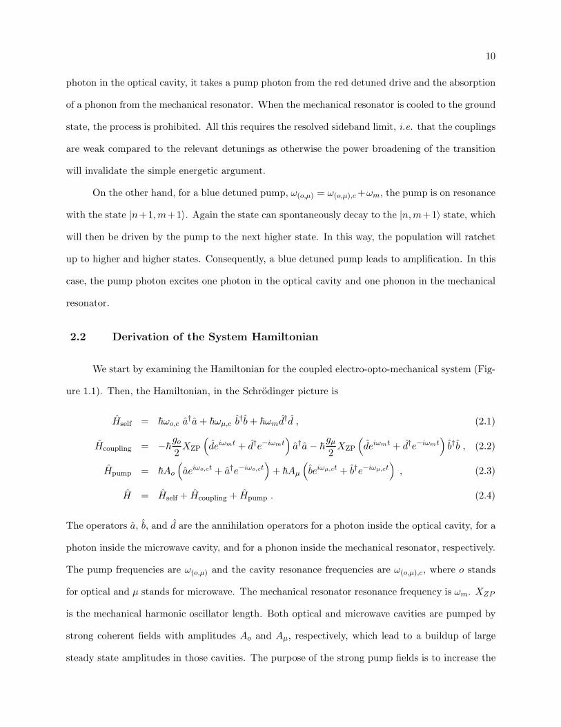
2.2 Derivation of the System Hamiltonian

We start by examining the Hamiltonian for the coupled electro-opto-mechanical system (Fig-

ure 1.1). Then, the Hamiltonian, in the Schrodinger picture is

Hself = ~ωo,c a†a+ ~ωµ,c b

†b+ ~ωmd†d , (2.1)

Hcoupling = −~go

2XZP

(

deiωmt + d†e−iωmt)

a†a− ~gµ

2XZP

(


b†b , (2.2)

Hpump = ~Ao

(

aeiωo,ct + a†e−iωo,ct)

+ ~Aµ

(

beiωµ,ct + b†e−iωµ,ct)

, (2.3)

H = Hself + Hcoupling + Hpump . (2.4)

The operators a, b, and d are the annihilation operators for a photon inside the optical cavity, for a

photon inside the microwave cavity, and for a phonon inside the mechanical resonator, respectively.

The pump frequencies are ω(o,µ) and the cavity resonance frequencies are ω(o,µ),c, where o stands

for optical and µ stands for microwave. The mechanical resonator resonance frequency is ωm. XZP

is the mechanical harmonic oscillator length. Both optical and microwave cavities are pumped by

strong coherent fields with amplitudes Ao and Aµ, respectively, which lead to a buildup of large

steady state amplitudes in those cavities. The purpose of the strong pump fields is to increase the

11

optomechanical coupling.

The strong coherent pump fields Ao and Aµ lead to a buildup of large steady state amplitudes

in the optical and microwave resonators. The steady state intracavity field amplitudes, in turn,

shift the equilibrium position of the mechanical resonator. The bare coupling constants go and gµ

are given by g(o,µ) = ∂∆o,µ/∂q where q is the position of the mechanical resonator and ∆o and ∆µ

are the resonance frequencies of the optical and microwave resonators in the frame rotating with

their respective pump frequencies.

First, we go into the interaction picture to explicitly show the dependence on the detuning

∆(o,µ) = ω(o,µ),c − ω(o,µ). We Define

Ho ≡~ωo a†a+ ~ωµ b

†b (2.5)

Vself =Hself − Ho

=~∆oa†a+ ~∆µb

†b+ ~ωmd†d . (2.6)

The other parts of the Hamiltonian remain unchanged so that the total interaction part of the

Hamiltonian is

V = Vself + Hcoupling + Hpump . (2.7)

The interaction Hamiltonian is then,

HI = e−iHotV eiHot . (2.8)

We use the Baker-Hausdorff theorem to simplify the exponentials,

eαX Y e−αX = Y + α[

X, Y]

+α2

2!

[

X,[

X, Y]]

+α3

3!

[

X,[

X,[

X, Y]]]

+ . . . . (2.9)

12

Thus, each operator is transformed in the following way,

e−iHot/~ a eiHot/~ = ae−iωot (2.10)

e−iHot/~ a† eiHot/~ = a†eiωot (2.11)

e−iHot/~ b eiHot/~ = be−iωµt (2.12)

e−iHot/~ b† eiHot/~ = b†eiωµt (2.13)

e−iHot/~ d eiHot/~ = d (2.14)

e−iHot/~ d† eiHot/~ = d† . (2.15)

Thus, for example, the optical pump term becomes,

~Aoe−iHot

(

aeiωo,ct + a†e−iωo,ct)

eiHot =~Ao

(

aei(ωo,c−ωo)t + a†e−i(ωo,c−ωo)t)

=~Ao

(

aei∆ot + a†e−i∆ot)

(2.16)

Applying the Baker-Hausdorff theorem to all the terms gives the full interaction Hamiltonian,

HI =~∆oa†a+ ~∆µb

†b+ ~ωmd†d

− ~go

2XZP

(


a†a− ~gµ

2XZP

(


b†b

+ ~Ao

(


+ ~Aµ

(

bei∆µt + b†e−i∆µt)

. (2.17)

The description of the system is greatly simplified by splitting off the steady state expectation

values of the various operators in the Hamiltonian Eq. (2.4) and by introducing fluctuations around

these means,

a→〈a〉SSei∆ot + a ,

b→〈b〉SSei∆µt + b . (2.18)

13

After removing the constant offset, the Hamiltonian to second order is,

Heff =~ [∆o〈a〉SS +Ao](


+ ~

[

∆µ〈b〉SS +Aµ

] (

bei∆µt + b†e−i∆µt)

− ~go

2XZP〈a〉2SS

(

de−iωmt + d†eiωmt)

− ~gµ

2XZP〈b〉2SS

(


+ ~∆oa†a+ ~∆µb

†b+ ~ωmd†d

− ~go

2XZP〈a〉SS

(

a†d†e−i(∆o+ωm)t + adei(∆o+ωm)t

+ ad†e−i(∆o−ωm)t + a†dei(∆o−ωm)t)

− ~gµ

2XZP〈b〉SS

(

b†d†e−i(∆µ+ωm)t + bdei(∆µ+ωm)t

+ bd†e−i(∆µ−ωm)t + b†dei(∆µ−ωm)t)

. (2.19)

By setting the linear terms equal to zero, we find that the steady state expectation values are

related to the pump amplitude and detuning,

〈a〉SS = − Ao

∆o, (2.20)

〈b〉SS = − Aµ

∆µ. (2.21)

With that, the Hamiltonian becomes,

Heff =~∆oa†a+ ~∆µb

†b+ ~ωmd†d

− ~Ωo

2〈a〉SS

(


− ~Ωµ

2〈b〉SS

(


− ~Ωo

2

(

a†d†e−i(∆o+ωm)t + adei(∆o+ωm)t + ad†e−i(∆o−ωm)t + a†dei(∆o−ωm)t)

− ~Ωµ

2

(

b†d†e−i(∆µ+ωm)t + bdei(∆µ+ωm)t + bd†e−i(∆µ−ωm)t + b†dei(∆µ−ωm)t)

, (2.22)

where the bare coupling constants have been modified to become

Ωo = − goXZPAo

∆o, (2.23)

Ωµ = − gµXZPAµ

∆µ. (2.24)

The highest experimental values have achieved about Ωo ∼ 0.1ωm and Ωµ ∼ 0.1ωm [39, 42] for

∆(o,µ) = ωm. It is important to note that the pump amplitude, A(o,µ) is a complex number

14

containing the relative phase of the pump field. Thus, the relative phase can be modified to change

the sign of the modified coupling constants. The magnitude of the coupling can be modified by

changing the bare coupling strength, the pump amplitude or the detuning.

2.3 Red Detuned System Hamiltonian

For the case where both the optical and microwave resonators are subject to a pump field

that is red detuned from their respective cavity resonance frequencies such that

∆o ≡ωo,c − ωo = ωm

∆µ ≡ωµ,c − ωµ = ωm , (2.25)

then, the Hamiltonian in Eq. 2.22 becomes,

Heff =~ωm

(

a†a+ b†b+ d†d)

− ~Ωo

2〈a〉SS

(


− ~Ωµ

2〈b〉SS

(


− ~Ωo

2

(

a†d†e−2iωmt + ade2iωmt + ad† + a†d)

− ~Ωµ

2

(

b†d†e−2iωmt + bde2iωmt + bd† + b†d)

. (2.26)

In the resolved sideband limit where the frequency, ωm, of the mechanical resonator is much

larger than the mechanical decay rate (as well as the effective coupling constants), we can employ

the rotating wave approximation where all the rapidly oscillating time dependent terms average to

zero, which leads to

Heff = ~ωm

(


− ~Ωo

2

(

a†d+ a d†)

− ~Ωµ

2

(

b†d+ b d†)

. (2.27)

This bilinear Hamiltonian is analogous to three quantized single mode fields coupled to each

other by beam splitters as illustrated in Figure 1.2. The beam splitters are adjustable. A coupling

of π/2 will be like a 50/50 beam splitter. A coupling of π will be like a mirror, swapping the states

perfectly. If we turn the coupling off, the oscillators will propagate freely as if there is no beam

15

splitter. Thus, by varying the coupling constants, we can change from 0 to 100% reflection and

transmission.

It is important to note that the quantum mechanical systems described by the field operators

a, b, and d are in fact fluctuations of the bare fields around their stationary values at each of their

respective resonator frequencies.

2.4 Blue Detuned System Hamiltonian

For the case where both the optical and microwave resonators are subject to a blue detuned

pump field such that,

∆o ≡ωo,c − ωo = −ωm

∆µ ≡ωµ,c − ωµ = −ωm , (2.28)

then the effective system Hamiltonian from Eq. 2.22 becomes,

Heff =~ωm

(

−a†a− b†b+ d†d)

− ~Ωo

2〈a〉SS

(


− ~Ωµ

2〈b〉SS

(


+ ~Ωo

2

(

a†de2iωmt + ad†e−2iωmt + ad+ a†d†)

+ ~Ωµ

2

(

b†de−2iωmt + bd†e2iωmt + bd+ b†d†)

. (2.29)

Applying the rotating wave approximation leads to the simple blue detuned effective Hamiltonian:

Heff = ~ωm

(

−a†a− b†b+ d†d)

+ ~Ωo

2

(

a†d† + ad)

+ ~Ωµ

2

(

b†d† + bd)

. (2.30)

Notice that unlike the red detuned case in which beam-splitter like coupling emerged, here the

Hamiltonian corresponds to creation or destruction of pairs of photons and phonons. This leads

to exponential growth or decay of the populations in each coupled system, and is reminiscent of

parametric amplification in nonlinear optical devices. Figure 2.2 shows the schematic diagram of

one such parametric amplifier.

16

ω1

ParametricCrystal

ω1 = ω

2 + ω

3

ω2

ω3

Figure 2.2: A schematic diagram of a parametric amplifier.

|1⟩

|2⟩

∆P ∆

S|3⟩γ ←

Pump Laserω

a

Stokes Laserω

b

Figure 2.3: Schematic of a three level atom showing the coupling needed for the STIRAP process.The Stokes coupling is turned on first. Then the pump coupling is turned on, resulting in statetransfer from state |1〉 to state |2〉 without leaving any population in state |3〉.

17

2.5 Analogy to Three Level Atom

Putting the Hamiltonian in Eq. 2.27 in matrix form reveals a remarkable similarity to the

Hamiltonian for a three level atom (Figure 2.3). Thus, the two systems may have similar behavior

in certain parameter regimes. This allows us to take insight from the quantum dynamics of few

level atomic systems and immediately understand certain aspects of the coupled microresonator

system.

We make an analogy between the states of a three level atom and the n = 1 states of each

resonator. We equate the atomic state |1〉 with having one photon in the microwave resonator,

state |2〉 with having one photon in the optical resonator, and state |3〉 with having one phonon in

the mechanical resonator. The self energy terms of the Hamiltonian in Eq. 2.27 are

Hself =~

∆µ 0 0

0 ∆o 0

0 0 ωm

. (2.31)

The interaction part of the Hamiltonian is

V = − 1

2~

0 0 Ωµ

0 0 Ωo

Ωµ Ωo 0

. (2.32)

We can diagonalize the matrix and find the Eigenstates and Eigenvalues [46].

H = ~ω+c†+c+ + ~ω−c

†−c− + ~ωoc

†oco (2.33)

where

c+ = − 1√2d− Ωoa+ Ωµb

√

2(

Ω2o + Ω2

µ

)

(2.34)

c− =1√2d− Ωoa+ Ωµb

√

2(

Ω2o + Ω2

µ

)

(2.35)

co =Ωµa− Ωob√

Ω2o + Ω2

µ

(2.36)

18

and

ω+ =ωm −√

Ω2o + Ω2

µ (2.37)

ω− =ωm +√

Ω2o + Ω2

µ (2.38)

ωo =ωm . (2.39)

There is a dark state associated with co that does not affect the state of the mechanical

resonator. We can adiabatically move a state in the microwave resonator to the optical resonator

by slowly varying the couplings without putting any population in the mechanical state. At the

beginning of the process, the optomechanical coupling is slowly turned on while the electromechan-

ical coupling is off so that the dark state is co = b. At the end of the process, the electromechanical

coupling is on, while the optomechanical coupling is off leaving the dark state in co = −a. This

effectively transduces the quantum state from the microwave cavity to the optical cavity.

This is similar to the Stimulated Raman Adiabatic Passage (STIRAP) process in a three

level atom. In the STIRAP process, the Stokes coupling (the coherent coupling between states |2〉

and |3〉) is turned on first which splits the energy levels for state |3〉. Then, the pump coupling (the

coherent coupling between states |1〉 and |3〉) is turned on and the population in state |1〉 is seen

to be transferred to state |2〉 without ever having any significant population in state |3〉 because of

the interference between the pathways corresponding to transversing each of the two split energy

levels. We will consider this adiabatic transduction process further in Ch. 6.

2.6 Fidelity

These Hamiltonians do not take into account the mechanical decoherence and thermal noise

that we would like to focus on throughout this thesis. In order to account for the thermal and

decay effects we use the Lagrangian in addition to the Hamiltonian.

L[ρ] =γmn

2

(

d†dρ+ ρd†d− 2dρd†)

+γm (n+ 1)

2

(

dd†ρ+ ρdd† − 2d†ρd)

, (2.40)

where γm is the decay rate of the mechanical resonator and n is the average occupation number of the

thermal bath. The Lagrangian makes an analytical solution impossible so, we need to numerically

19

simulate the evolution of the system under the influence of mechanical decay and thermal noise.

We will look more at the numerical methods we employ in Ch. 4. But here, we look at the fidelity

measure [40] that we will use to quantitatively measure the success of the schemes we explore in

this thesis. We look at the fidelity [40] for retrieving the input state after storage or transfer as a

function of the mechanical quality factor, Qm = ωm/γm. The fidelity [41] we employ is defined as

F (ρi, ρf ) ≡[

Tr

(

√√ρiρf

√ρi

)]2

(2.41)

where ρi and ρf are the reduced density matrices for the input and output states respectively.

To calculate this more easily in our numerical simulations, we convert this equation to an

eigenvalue equation. We set M =√ρiρf

√ρi and the fidelity becomes F = [Tr

√M ]2. We find the

eigenvalues λi of M by a unitary transformation U such that UMU−1 = M ′ and

M ′ =

λ1 0 . . .

0 λ2 . . .

......

. . .

. (2.42)

The fidelity formula is now

F =[

TrU√MU−1

]2

=[

Tr√UMU−1

]2

=[

Tr√M ′]2

=

[

∑

i

√

λi

]2

. (2.43)

We next show that the fidelity function has the anticipated properties [18]. Since ρ is positive

definite, we can easily see that the fidelity is also positive definite. Also, ρ has strictly positive

eigenvalues that are less than 1, and so 0 ≤ F ≤ 1. The upper limit 1 corresponds to perfect

replication of the quantum state, while small values of F indicate significant degradation. For

20

ρi = ρf , we want the fidelity to equal 1, which is true since

F =

[

Tr

(

√√ρiρi

√ρi

)]2

=

[

Tr

(

√

ρ2i

)]2

= [Tr ρi]2

=1 . (2.44)

A special simplification occurs for pure states where the fidelity reduces to an overlap func-

tional:

F =

[

Tr

(

√√ρiρf

√ρi

)]2

=[

Tr(√ρiρfρi

)]2

=

[

Tr

(

√

|ψi〉〈ψi|ψf 〉〈ψf |ψi〉〈ψi|)]2

= [Tr (|〈ψi|ψf 〉|ρi)]2

=|〈ψi|ψf 〉|2 . (2.45)

2.7 Summary

In this chapter, we have developed a toolbox that we will use throughout this thesis. We have

derived the red and blue detuned linearized Hamiltonians for the system of three coupled harmonic

resonators. The energetic properties of the Hamiltonians shows the cooling and heating effects in

the system. The Eigenstates and Eigenvalues of the red detuned Hamiltonian are very similar to

those of a three level atom. Also, we defined the fidelity function that we will use to quantitatively

measure the success of the schemes presented in future chapters.

Chapter 3

Transduction and Quantum Memory in a Coherent State Basis

3.1 Transduction

To illustrate many of the concepts we will explore in this thesis, we will first look at the

solution in the classical regime by working exclusively with coherent states. In this case, the three

coupled harmonic resonator system may be solved analytically. This provides a reference for the

full quantum solutions that we consider later in the thesis.

We will assume that the initial state in the microwave resonator is |β(t = 0)〉 with the other

resonators starting in the vacuum |0〉 state. We also assume that the transduction occurs from the

microwave resonator to the optical resonator. The output state is then |α(tf )〉.

If all the oscillators, mechanical, microwave, and optical are in coherent states, the eigenstates

for each resonator subsystem are given by

a|α〉 =α|α〉 (3.1)

b|β〉 =β|β〉 (3.2)

d|δ〉 =δ|δ〉 . (3.3)

In addition, the initial quantum state of the full system is the tensor product of the individual

resonator states, i.e.,

|Ψ〉 = |α〉 ⊗ |β〉 ⊗ |δ〉 . (3.4)

22

3.1.1 Equations of Motion

To derive the equations of motion for the system, we start with the linearized Hamiltonian

given in Eq. 2.27.

H = ~ωm

(


− ~Ωo

2

(

a†d+ d†a)

− ~Ωµ

2

(

b†d+ d†b)

(3.5)

The time derivative of each operator is given by the Heisenberg equation.

da(t)

dt=

1

i~

[

a, H]

(3.6)

d〈Ψ(t)|a|Ψ(t)〉dt

=1

i~〈Ψ(t)|

[

a, H]

|Ψ(t)〉 (3.7)

dα(t)

dt=〈Ψ(t)|

(

−iωma+ iΩo

2d

)

|Ψ(t)〉 (3.8)

α(t) = − iωmα(t) + iΩo

2δ(t) . (3.9)

The other subsystem equations are performed in the same manner,

β(t) = − iωmβ(t) + iΩµ

2δ(t) (3.10)

δ(t) = − iωmδ(t) + iΩo

2α(t) + i

Ωµ

2β(t) . (3.11)

3.1.2 Constant Coupling

In the case where the couplings are constant, the equations of motion 3.9- 3.11 can be solved

analytically. The solution is

α(t) =e−iωmt

Ω2

(

Ωµ (Ωµα(0) − Ωoβ(0)) + Ωo (Ωoα(0) + Ωµβ(0)) cos

(

Ωt

2

)

+ iΩoΩδ(0) sin

(

Ωt

2

))

(3.12)

β(t) =e−iωmt

Ω2

(

Ωo (Ωoβ(0) − Ωµα(0)) + Ωµ (Ωoα(0) + Ωµβ(0)) cos

(

Ωt

2

)

+ iΩµΩδ(0) sin

(

Ωt

2

))

(3.13)

δ(t) =e−iωmt

Ω2

(

Ωδ(0) cos

(

Ωt

2

)

+ i (Ωoα(0) + Ωµβ(0)) sin

(

Ωt

2

))

(3.14)

23

where Ω =√

Ω2o + Ω2

µ is the Rabi frequency. For our set of initial conditions, α(0) = 0 and δ(0) = 0,

the equations reduce to

α(t) =e−iωmt

Ω2

(

−ΩoΩµβ(0) + ΩoΩµβ(0) cos

(

Ωt

2

))

(3.15)

β(t) =e−iωmt

Ω2

(

Ω2oβ(0) + Ω2

µβ(0) cos

(

Ωt

2

))

(3.16)

δ(t) =ie−iωmt

Ω2Ωµβ(0) sin

(

Ωt

2

)

. (3.17)

Figure 3.1 illustrates the normal Rabi flopping that occurs when the resonators are coupled

with a constant coupling. For the electromechanical system shown in Figure 3.1(A), the Rabi

frequency reduces to Ω = Ωµ. For the electro-optomechanical system shown in Figure 3.1(B), the

Rabi frequency reduces to Ω =√

2Ωµ, where we have set Ωo = Ωµ.

In order to get transduction in this system, we need to have two pulses. The first π pulse,

which we take to have a square profile, will swap the state from the microwave resonator into the

mechanical resonator. Then the second π pulse, also taken to be square, will swap the state into

the optical resonator. This is shown in Figure 3.2. The time needed for this transfer is thus 2π/Ωµ.

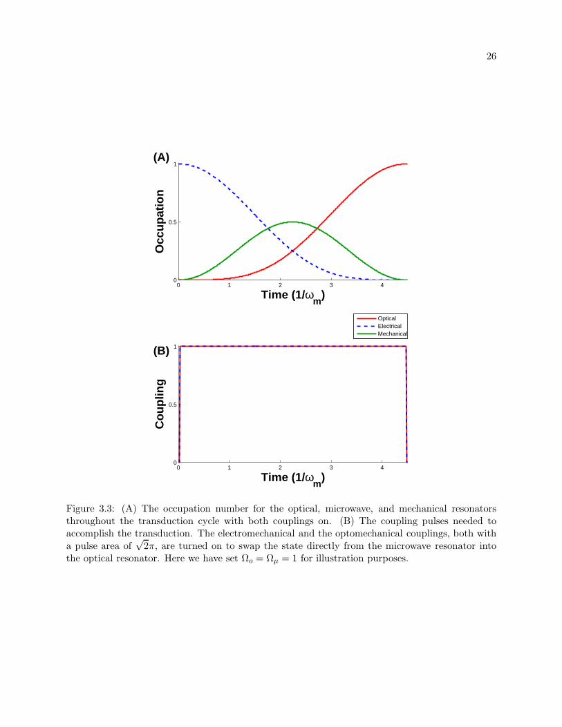
However, if both couplings are on at the same time, as we saw in Figure 3.1(B), the Rabi

frequency is increased to√

2Ωµ. Thus the pulse area needed for the swapping pulses increases to

√2π. The total transfer time is now

√2π/Ωµ as shown in Figure 3.3. Also note that here the

state is transferred directly from the microwave resonator to the optical resonator without fully

populating the mechanical resonator.

3.1.3 Analytic Fidelity Formula

In general, the fidelity in the coherent state basis, is just the overlap between the two Gaussian

states [40],

F = |〈α(tf )|β(0)〉|2 , (3.18)

since the oscillator states remain pure rather than mixed by assumption. For the coherent case,

the initial state is |β(0)〉 representing the state in the microwave resonator. The final state will be

24

0 2 4 6 8 10 12 14 16 180

0.5

1O

ccup

atio

n

Time (1/ωm

)

0 2 4 6 8 10 12 14 16 180

0.5

1

Occ

upat

ion

Time (1/ωm

)

(A)

(B)

OpticalElectricalMechanical

Figure 3.1: The occupation numbers of each resonator swap back and forth at the Rabi frequencywhen the coupling between the resonators is kept constant. The initial state in the microwaveresonator is β(0) = 1. (A) The case for two coupled resonators such as in the electromechanicalsystem. (B) The case for three coupled resonators such as the electro-optomechanical system. Herewe have set Ωo = Ωµ = 1.

25

0 1 2 3 4 5 60

0.5

1O

ccup

atio

n

Time (1/ωm

)


0 1 2 3 4 5 60

0.5

1

Cou

plin

g

Time (1/ωm

)

(A)

(B)

Figure 3.2: (A) The occupation number for the optical, microwave, and mechanical resonatorsthroughout the transduction cycle with each coupling turned on in sequence. (B) The couplingpulses needed to accomplish the transduction. First the electromechanical coupling, with a pulsearea of π, is turned on to swap the state from the microwave resonator into the mechanical resonator.Then the optomechanical coupling, also with a pulse area of π, is turned on to swap the state intothe optical resonator. Here we have set Ωo = Ωµ = 1 for illustration purposes.

26

0 1 2 3 40

0.5

1O

ccup

atio

n

Time (1/ωm

)


0 1 2 3 40

0.5

1

Cou

plin

g

Time (1/ωm

)

(A)

(B)

Figure 3.3: (A) The occupation number for the optical, microwave, and mechanical resonatorsthroughout the transduction cycle with both couplings on. (B) The coupling pulses needed toaccomplish the transduction. The electromechanical and the optomechanical couplings, both witha pulse area of

√2π, are turned on to swap the state directly from the microwave resonator into

the optical resonator. Here we have set Ωo = Ωµ = 1 for illustration purposes.

27

|α(tf )〉 representing the final state in the optical resonator for quantum transduction and the final

state in the microwave resonator for quantum memory.

At zero temperature, in the case where the pulse duration is short compared to the decay time

of the mechanical resonator, we can neglect the decay during the swapping pulses and assume that

the swaps happened perfectly. In that case, the final state will only have decayed exponentially,

at the mechanical decay rate γm, during the time, ∆T , between the two π pulses to become

|ψf 〉 = |e−γm∆T/2β(0)〉. Thus we can analytically find the fidelity for a pure final state to be

F = |〈e−ωm∆T2Qm β(0)|β(0)〉|2 = e−|β(0)|2(1−e−ωm∆T/(2Qm))2 . (3.19)

However, for non-zero temperatures or large decay rates the final state will thermalize quickly

and this formula will no longer be valid. The state does not decay to the vacuum as Eq. (3.19)

suggests. Rather it decays to a thermalized value. Thus, the final fidelity for pure states will

saturate at low-Q to the overlap between a thermalized state and the initial state. Thus, the

coherent state fidelity (Figure 3.4) takes on the form,

F (Q) = F (0) + (1 − F (0)) e−|β(0)|2(1−e−ωm∆T/(2Qm))2 . (3.20)

where F (0) is the thermal saturation overlap value.

Further complicating matters, the full density matrix, which is pure, must be reduced to

the resonator subsystem that is being read out before taking the fidelity overlap with the reduced

input density matrix. This makes the reduced density matrices impure. Consequently, we need to

employ the more general formula to find the fidelity that is valid for states that are not pure.

3.1.4 Pulsed Coupling

Square pulses have a sinc squared frequency composition, and thus a significant contribution

from high frequency components. Now we use Gaussian pulses for the coupling parameters so

we can look at more sophisticated pulse sequences that have a smoother and localized frequency

28

100

101

102

103

104

0.5

0.75

1

Fid

elity

Qm

Figure 3.4: The fidelity from Eq. 3.20 as a function of mechanical resonator quality, Qm. Here∆T = 64(1/ωm) and F (0) = 0.25.

29

decomposition;

Ωo(t) =Ωo(to)e− (t−to)2

w2oπ (3.21)

Ωµ(t) =Ωµ(tµ)e− (t−tµ)2

w2µπ (3.22)

where Ωo(to) and Ωµ(tµ) are the pulse amplitudes and wo and wµ are the pulse widths. For

simplicity, we set the amplitudes and widths equal (Ωo(to) = Ωµ(tµ) = Ω and wo = wµ = w) so

both coupling pulses have the same shape. The only difference will be the location of the center of

the Gaussian pulses. The pulse area of either coupling pulse is then given by wΩπ.

The equations of motion 3.9-3.11 cannot be solved analytically in any simple way. We nu-

merically solve the equations for a variety of relative pulse centers and widths. We sweep the pulse

centers from the point where the two coupling pulses are completely separated with the microwave

pulse occurring first to the point where they are occurring simultaneously. This allows us to com-

pare with the results of section 3.1.2. Then, we continue the sweep with the optical pulse occurring

first until the pulses are completely separated again. We do this for a variety of pulse areas, while

keeping Ω constant.

Figure 3.5 shows the fidelity across the sweeps when the reservoir to which the mechanical

resonator is coupled to is at zero temperature. This allows us to neglect decay and thermal noise

processes in our analysis. The zero on the x axis is the point where the two coupling pulses are

occurring simultaneously. The positive x values indicate the separation between the peaks of the

two coupling pulses that are intuitive, i.e., the electromechanical coupling pulse occurs before the

optomechanical coupling pulse. The negative x values indicate the separation between the peaks of

the two coupling pulses that are counter-intuitive, i.e., the optomechanical coupling pulse occurs

before the electromechanical coupling pulse.

As the pulses move farther apart, they eventually become effectively separated and the dis-

tance between them no longer matters (since there is no decay here). This is the area on the lower

right-hand side of the plot where the fidelity peaks level off at multiples of π. Pulses that are π

pulses or an odd integer multiple of a π pulse will swap the state completely from the microwave

30

-20 -10 0 10 20

1

2

3

4

5

Pulse Separa tion H%T m axL

Puls

eA

reaHΠL

Coherent State Tranduction Fidelity

0

0.4

0.5

0.7

0.9

0.95

0.99

Figure 3.5: The fidelity vs. pulse width and pulse separation for Qm = 10000 and n = 0.

31

resonator to the optical resonator. Any other pulse area will not perfectly swap the states. Thus,

we see the periodic behavior we expect in that part of the plot in analogy with Rabi oscillations.

At zero pulse separation, the pulses are identical and the Rabi swapping pulse area is√

2π.

Thus, the peak fidelity periods are at odd integer multiples of√

2π. For partially overlapping intu-

itive pulses, the peak fidelity periods smoothly drop from the simultaneous values to the separated

values.

The lower left-hand side of the plot is where the counter-intuitive pulses have gotten far

enough apart to be effectively separated and thus no transduction is occurring. However, when

the counter-intuitive pulses are partially overlapping, we see a large area of high fidelity with

no oscillatory behavior. This corresponds to the optomechanical implementation of the STIRAP

process more usually seen in a three-level atom system as we discussed in section 2.5. Each state in

the Fermionic three level atom is analogous to a ladder of Boson states in each harmonic resonator.

Instead of having a population of 0 or 1 in each of the three states, there can be any population in

each state. The fact that the STIRAP process is evident in a Bosonic system consisting of coupled

resonators with a Hilbert space dimension much larger than three, rather than in a Fermionic

system of only three levels is significant. As the pulse area increases, the pulses become more and

more adiabatic and the separation and pulse area of the pulses becomes more and more irrelevant.

3.2 Memory: Quantum Information Storage and Retrieval

Now we reduce the system to two coupled harmonic resonators to study the quantum memory

case. This is equivalent to setting Ωo = 0 so that we are only looking at the electromechanical

subsystem. The initial state is still |β(0)〉 in the microwave resonator and |0〉 in the mechanical

resonator. However the coupling pulses will now swap the state into the mechanical resonator and

then back to the microwave resonator. We want to explore how long the state can be stored in the

mechanical resonator before significant degradation occurs.

32

3.2.1 Equations of Motion

The reduced equations of motion for the coherent amplitudes are

β(t) = − iωmβ(t) + iΩµ

2δ(t) (3.23)

δ(t) = − iωmδ(t) + iΩµ

2β(t) − γm

2δ(t) . (3.24)

The solutions for the constant coupling are now,

β(t) =e−(iωm+γm/4)t

(

β(0) cos

(

Ω

2t

)

+β(0)γm + 2iδ(0)Ωµ

2Ωsin

(

Ω

2t

))

(3.25)

δ(t) =e−(iωm+γm/4)t

(

δ(0) cos

(

Ω

2t

)

+−δ(0)γm + 2iβ(0)Ωµ

2Ωsin

(

Ω

2t

))

(3.26)

where Ω =√

Ω2µ − γ2

m/4.

3.2.2 Storage Time

For the case of strong short π/2 pulses, the decay can be neglected during the pulses, so that

the final state only depends on the length of time between the storage and retrieval pulses, ∆T and

the decay rate,

β(∆T ) = β(0)e−iωm∆T e−γm∆T/2 . (3.27)

This gives us the same fidelity that we found in Eq. 3.19.

In Figure 3.6 we plot the fidelity for three different Qm = ωm/γm values vs. the storage

time ∆T . In subplot (A), we see that the fidelity decays exponentially with the storage time at a

rate determined by Qm as expected. In subplot (B), we show the same fidelity versus the storage

time scaled by the mechanical resonator quality. When the axes are scaled like this, all the curves

collapse onto a universal curve:

F = e−|β(0)|2(1−e−ζo/2)2 (3.28)

where ζo = ωm∆T/Qm.

33

0 200 400 600 800 10000.5

0.75

1

∆ T (1/ωm

)

Fid

elity

Qm

= 10

Qm

= 100

Qm

= 1000

0 5 10 15 20 250.5

0.75

1

∆ T/Qm

(1/ωm

)

Fid

elity

(A)

(B)Q

m = 10

Qm

= 100

Qm

= 1000

Figure 3.6: (A) The fidelity decays for longer storage times and lower mechanical quality. (B) Thesame fidelity scaled by the mechanical quality so that all curves collapse onto one universal curveF = e−|β(0)|2(1−e−ζo/2)2 where ζo = ωm∆T/Qm. Here β(0) = 1.

34

3.3 Summary

We illustrated many of the concepts we will use throughout this thesis by working exclusively

with coherent states for a zero temperature bath. We looked at the fidelity for transduction with

separated, simultaneous, and adiabatic transfer schemes. We will explore these protocols further

with other quantum states in Ch. 6. We also looked at the fidelity for quantum memory versus

storage time and found a universal curve for how the fidelity decays. We will further explore

quantum memory with other quantum states in Ch. 5.

Chapter 4

Quantum State Diffusion

4.1 QSD Algorithm

We use the quantum state diffusion (QSD) method to simulate the fully quantum evolution

of this open system [12, 28, 4, 48]. The QSD method is well suited for this problem because it

yields the conditional evolution of an open quantum system subject to homodyne measurements

of the output fields. In this way, we may obtain amplitude and phase information about the

decay channel. In the QSD approach, we stochastically evolve each resonator subsystem as if we

were performing a continuous fictitious homodyne measurement of the photons or phonons coming

out of each resonator. Even though an actual experiment can not measure the phonons in the

mechanical resonator, the numerical simulation gives us access to this information in the spirit of a

‘Gedanken’ measurement. For the scenarios we explore, the decay rates of the optical and microwave

resonators are set to zero, so that only the mechanical resonator is coupled to the environment.

Thus, in those cases, the stochastic evolution only applies to the mechanical resonator subsystem,

while the optical and microwave resonators evolve according to the Schrodinger equation. In actual

experiments, the optical and microwave resonators are also coupled to the environment and actual

homodyne measurements can be performed on those output fields. The QSD method works for the

fully open system as well. But in this thesis, we are reducing the fully open system to focus only

on the mechanical decoherence.

36

The total state of the system is the tensor product of the states of each resonator subsystem

|Ψ(t)〉 = |ψa(t)〉 ⊗ |ψb(t)〉 ⊗ |ψd(t)〉 (4.1)

if the subsystems are not entangled with each other. We construct the initial total state of the

system in this way. Then, we evolve the total state according to the QSD algorithm, which has the

effect of entangling the subsystem states.

In the QSD method, the evolution of the total density matrix of the system is unraveled into

an ensemble of stochastic parallel pure state trajectories. Each trajectory is evolved according to a

stochastic differential equation. The trajectories are then averaged in the ensemble sense to recreate

the total density matrix. In the limit of a large number of trajectories, the ensemble average of the

stochastic trajectories goes to a state diffusion evolution. Each trajectory evolves according to the

stochastic differential equation [48]

|Ψ(t+ dt)〉 =

1 −[γm(2n + 1)

2d†d+ 2γm(2n+ 1)〈d† + d〉d+

i

~Heff

]

dt

+ d√γmn dWd(t) + d†

√

γm(n+ 1) dWd†(t)

|Ψ(t)〉 (4.2)

where, dW (t) is the continuum limit of a Wiener increment, ∆W , which satisfies the ensemble

average 〈(∆W )2〉 = ∆t of a Gaussian random distribution with a width ∆t. There are two Wiener

increments, one for each noise process in the mechanical oscillator where there are two types of

decay channels, one for phonons entering the system and one for phonons leaving the system. The

stochastic evolution is not Hermitian and thus does not preserve the norm of the state. So, the

new total state must also be normalized at each time step in the numerical integration.

The SDE can be rewritten in the form,

|Ψ(t+ dt)〉 =

[

1 − A dt +∑

i

BidWi(t)

]

|Ψ(t)〉 (4.3)

which is the starting point for the multidimensional second order weak scheme given in reference [21]

on page 486 that we use to implement the QSD method in the C++ programming language.

37

4.2 Test Cases

We used several test cases to validate our approach and computational implementation. We

looked at the two level atom case, the case of one thermal harmonic oscillator, the case of cooling

the mechanical oscillator with a red detuned pump, and the case of heating with a blue detuned

pump.

4.2.1 Two Level Atom

First, we compared the numerical results with the known solution for a two level atom where

the effective Hamiltonian is

Heff = ∆σz + Ω (σ+ + σ−) − iγ

2σ+σ− , (4.4)

where ∆ is the detuning, Ω is the Rabi frequency, γ is the spontaneous decay rate from the excited

state to the ground state, and σ+, σ−, and σz are the Pauli spin matrices. The solution to the

optical Bloch equations that results from this Hamiltonian for the excited state probability of a

two-level atom is [15]

ρee =2Ω2

γ2/2 + 4Ω2

(

1 −(

cos(λt) +3γ

4λsin(λt)

)

e−3γt/4

)

(4.5)

where λ =√

4Ω2 − γ2/16.

Figure 4.1(A) shows the first 10 individual trajectories for the excited state probability from

the QSD simulation. The average of the first 10 trajectories is shown by the thick black line. All 4000

trajectories in the simulation average to the final excited state probability shown in Figure 4.1(B).

Figure 4.1(B) shows numerical results for the probability of being in the excited state compared

with the analytic solution of the optical Bloch equations when the atom is initially in the ground

state. We ran 4000 trajectories and set Ω = 3γ.

As we increase the number of trajectories, we would expect the noise for a second order

weak scheme to decrease like 1/√n where n is the number of trajectories, which is what we see in

Figure 4.2.

38

0 0.5 1 1.5 2 2.5 3 3.5 40

0.1

0.2

0.3

0.4

0.5

0.6

0.7

0.8

0.9

1

Time (1/γ)

Pro

babi

lity

Two Level Atom Excited State Probability

0 0.5 1 1.5 2 2.5 3 3.5 40

0.1

0.2

0.3

0.4

0.5

0.6

0.7

0.8

0.9

Time (1/γ)

Pro

babi

lity

Ω= 3γ

(A)

(B)Optical Bloch Equation4000 Ensemble QSD Simulation

Figure 4.1: Two Level Atom Excited State Population. (A) The first 10 individual trajectoriesfrom the QSD simulation. The average of the first 10 trajectories is shown by the thick black line.(B) The excited state population of a two level atom from the numerical simulation (solid blueline) compared with the analytic solution from the optical Bloch equations (dashed black line) forthe case of Ω = 3γ for 4000 trajectories.

39

100

101

102

103

104

10−2

10−1

100

Noi

se

Number of Trajectories

1/√

nNoise

Figure 4.2: The noise decreases with the number of trajectories like 1/√n where n is the number

of trajectories.

40

4.2.2 One Harmonic Oscillator

Next, we looked at the expected behavior for one thermal harmonic resonator. We ran three

cases with 400 trajectories each to test the different aspects of the numerical implementation.

The first case is a harmonic resonator that was already thermalized to the temperature of

the thermal bath. The initial state used here is a Fock state, |n = 3〉. In this case, we expect the

occupation number of the resonator to remain constant at the thermal bath temperature, which

corresponds to an n = 3 thermal state here. This is exactly what we see in Figure 4.3(A).

The second case is a harmonic resonator that is initially occupied at n = 3, but is connected to

a zero temperature bath. In this case, we expect to see the occupation number decay exponentially

to the bath temperature, as illustrated by our results in Figure 4.3(B).

The third case is a harmonic resonator that is initially empty (n = 0) and is connected to

a bath with temperature corresponding to a thermal occupancy of n = 2. In this case, we expect

the occupation number to exponentially increase at a rate determined by γmn until the resonator

thermalizes with the bath. This is what we observed, as shown in Figure 4.3(C).

4.2.3 Sideband Cooling

Next, we looked at two and three coupled harmonic resonators with a red detuned pump

field, where only the mechanical resonator is coupled to a thermal bath. In this case, we get cooling

of the mechanical resonator as we saw in Section 2.1 The mechanical resonator is losing phonons

to decay and to the other resonators, but it is also gaining phonons from the thermal bath. So the

final equilibrium temperature will be non-zero.

Figure 4.4(A) shows the cooling for the electromechanical system for 500 trajectories in the

case where γm = γµ. As the two resonators come into equilibrium with each other they arrive at

equal steady-state occupation numbers which is approximately half of the thermal bath temperature

n = 3. This is because the state spends approximately half of the time in the mechanical resonator

where it can be affected by the thermal bath. Also, the rate of phonons being absorbed from the

41

0 50 100 150 200 250 300 350 400 450 5000

1

2

3

Occ

upat

ion

Thermal Harmonic Oscillator

0 50 100 150 200 250 300 350 400 450 5000

1

2

3

Occ

upat

ion

0 50 100 150 200 250 300 350 400 450 5000

1

2

3

Time (1/ωm

)

Occ

upat

ion

(A)

(B)

(C)

Figure 4.3: The occupation number of one thermal harmonic resonator (blue line) vs. the theoreticalprediction (black line). (A) The case where the resonator starts out thermalized to the bathtemperature corresponding to n = n = 3 and thus remains at that temperature. (B) The casewhere the resonator is initially occupied at n = 3 but is connected to a zero temperature bath andthus decays to zero temperature. (C) The case where the resonator is initially empty (n = 0) andis connected to a hotter bath with temperature corresponding to n = 2 and thus exponentiallyincreases until it thermalizes with the bath. The number of trajectories used in all these cases was400.

42

0 10 20 30 40 50 60 70 80 90 1000

1

2

3O

ccup

atio

n

Steady State Values:Electrical: 1.5

Mechanical: 1.5

ElectricalMechanical

0 10 20 30 40 50 60 70 80 90 1000

1

2

3

Occ

upat

ion

Time (1/ωm

)

Steady State Values:Optical: 0.76

Electrical: 0.76Mechanical: 1.5

(A)

(B)OpticalElectricalMechanical

Figure 4.4: Cooling coupled harmonic resonators for 500 trajectories. (A) The case for an elec-tromechanical system where γm = γµ. (B) The case for an electro-opto-mechanical system whereγm = γµ = γo. In both cases, the thermal bath temperature corresponds to n = 3.

43

thermal bath is equal to the rate of phonons being transduced to photons in the microwave cavity

where they are lost to the zero temperature bath.

Figure 4.4(B) shows the cooling for the electro-opto-mechanical system for 500 trajectories

where γ(o,µ) = γm. We have set the electromechanical coupling to be equal to the optomechanical

coupling. Thus, the steady state occupation of the microwave and optical resonators is half of the

occupation of the mechanical resonator because the phonons are transferred at equal rates into

each of the other two resonators.

In contrast, Figure 4.5 shows the cases for two (subplot (A)) and three (subplot (B)) coupled

resonators where γ(o,µ) ≫ γm. In these cases, the state will decay out of the microwave and optical

cavities much faster than the mechanical resonator is absorbing phonons from its thermal bath. So

the mechanical resonator will cool to its ground state.

4.2.4 Blue Detuned Pump

Next, we look at the case of a blue detuned pump field with two coupled resonators. In

this case, we expect exponential heating in both resonators. From the Hamiltonian, Eq. 2.30, we

expect correlated pairs of photons and phonons to be generated. Figure 4.6(A) shows the occupation

numbers for both resonators growing exponentially with a zero number difference for positive values

of the coupling strength and decaying exponentially for negative values of the coupling strength.

Subplot (B) shows the coupling strength. Setting the coupling to be negative is equivalent to time

reversal, so the observation of decay can be anticipated. Subplot (C) shows that the variance of the

number difference is zero for all times, indicating that photons/phonons are produced in correlated

pairs at all times.

4.3 Summary

The Quantum State Diffusion method is a versatile way to unravel the density matrix master

equation into pure state trajectories that can be evolved independently. The total state is found

by the ensemble average of these individual trajectories. We found that the QSD approach was

44

0 10 20 30 40 50 60 70 80 90 1000

1

2

3

Occ

upat

ion


0 10 20 30 40 50 60 70 80 90 1000

1

2

3

Occ

upat

ion

Time (1/ωm

)

(A)

(B)OpticalElectricalMechanical

Figure 4.5: Cooling coupled harmonic resonators to the ground state. (A) The case for an elec-tromechanical system where γµ ≫ γm. (B) The case for an electro-opto-mechanical system whereγ(o,µ) ≫ γm. In both cases, the thermal bath temperature corresponds to n = 3.

45

0 5 10 15 20 25 30 35 400

0.5

1

1.5

2O

ccup

atio

n


5 10 15 20 25 30 35

−0.1

0

0.1

Ω

0 5 10 15 20 25 30 35 400

0.2

0.4

0.6

0.8

1

Var

ianc

e

Time (1/ωm

)

(A)

(B)

(C)

Figure 4.6: Blue Detuned Occupation and Variance. (A) The number of photons/phonons in eachresonator. (B) The coupling strength. When the coupling is positive, the number grows expo-nentially. When it is negative, it decays exponentially, until it hits zero, then grows exponentially

again. (C) The variance in the number difference, ∆w = 〈(

b†b− d†d)2

〉−(

〈b†b〉 − 〈d†d〉)2

, remains

zero indicating that photons/phonons are produced in correlated pairs at all times.

46

particularly suited to our system of three coupled harmonic resonators. We used several test cases

to verify that our computational implementation of the QSD method was done correctly.

Chapter 5

Quantum Memory: Storage and Retrieval

One of the possible applications of this system is to store a quantum state in the mechanical

resonator. One could prepare the microwave resonator in any of a variety of quantum states. This

can be done with superconducting quantum circuits or other experimental setups such as those

described in [22, 19, 43, 14]. Then, the states of the microwave and mechanical resonators could be

swapped using a “π-pulse”, effectively storing the quantum state in the mechanical resonator. At

some later time, another swap could be done to put the state back into the microwave resonator

where it can be retrieved [49, 40]. The objective would be to maintain high fidelity of the quantum

state involved. These swaps are achieved by varying the coupling constant, Ω(o,µ) which behaves

like a Rabi frequency in the beam splitter Hamiltonian, Eq. 2.27. As we saw in Eqs. 2.23 and 2.24,

the coupling constants can be changed by modulating the bare coupling constants g(o,µ) or the

pump amplitude A(o,µ), or the detuning ∆(o,µ). For this problem, it is sufficient to consider just

a pair of resonators. We reduce the system to one electromagnetic resonator and one mechanical

resonator by setting one of the coupling constants to zero.

A “π-pulse” in this context is a pulse where the time integral over the coupling constant in

frequency units is π. For the Gaussian coupling pulses, Ω(t) = Ωe−(t−tc)2/(w2π), that we employ, the

pulse area is wπΩ where wπ is the width of the Gaussian and the peak amplitude is Ω. The pulse

sequence is schematically shown in Figure 5.1(A). The first π pulse is the storage pulse. The second

π pulse is the retrieval pulse. The sign of the coupling constant for retrieval must be the opposite

of the sign for storage in order to cancel the phase accumulation during the pulses. Also, the width

48

0 50 100 150 200 250 300

0

∆T

Ω

Time (1/ωm

)

0 50 100 150 200 250 3000

0.5

Occ

upat

ion

Time (1/ωm

)

(A)

(B)

Figure 5.1: Quantum memory pulse sequence and occupation for the case of ∆T = 160(1/ωm). (A)A schematic diagram of the coupling π pulse sequence for Quantum State Memory tests. The signof the coupling constant for retrieval must be the opposite of the sign for storage in order to cancelthe phase accumulation during the pulses. (B) The occupation numbers for the microwave andmechanical resonators throughout the memory pulse sequence. The actual storage time is reducedby the width of the Gaussian pulses.

49

of the π pulse must be short compared to the mechanical decay rate γm otherwise, the state may

decay before it can be swapped to the other resonator. Subplot (B) shows the occupation numbers

of both resonators throughout the sequence. The first pulse swaps the state from the microwave

resonator to the mechanical resonator. The second pulse swaps the state back into the microwave

resonator. It takes approximately the width of the π pulse before the state is fully in the mechanical

resonator. Thus, the actual storage time of the state in the mechanical resonator is approximately

the separation time between the peaks of the pulses (∆T ) reduced by the width of the pulses.

If we move the pulses as close together as possible (shown in Figure 5.2 for ∆T = 64(1/ωm)),

then the peak separation ∆T will be approximately twice the width of the Gaussian π pulses. Even

though there is no time between the end of the storage pulse and the beginning of the retrieval

pulse, the state is still in the mechanical resonator for approximately the width of the π pulse,

which for all the quantum memory cases is wπ = π/Ωµ = π/(0.1ωm).

To see how well the system is able to store classical and quantum states, we study a variety

of initial states with the same pulse sequence for storage and retrieval. Recall that these states in

fact represent the phonon or photon fluctuations around the stationary value of each resonator, as

we have previously described in the derivation of the linearized effective Hamiltonian, Eq. 2.27.

We use coherent states |α〉|n〉m, squeezed coherent states |α, ξ〉|n〉m, cat states |ψcat〉, and a

superposition of Fock states |ψSF 〉 as inputs to the microwave resonator. The squeezed coherent

state [44] is a displaced squeezed vacuum state, |α, ξ〉 = D(α)S(ξ)|0〉, where α is the mean value

and ξ is the squeezing parameter. The displacement operator is D(α) = eαa†−α∗a and the squeezing

operator is S(ξ) = e12(ξ∗a2−ξ(a†)2).

The cat state is |ψcat〉 = N(|α〉+ |−α〉)|n〉m where N is a normalization constant. The input

state for the superposition of Fock states that we will study is |ψSF 〉 = 1√2(|0〉µ + |1〉µ)|n〉m, where

|i〉µ indicates the photon fluctuations around the stationary value inside the microwave cavity and

|n〉m indicates the phonon fluctuations around the stationary value inside the mechanical resonator.

The initial Fock state for the mechanical resonator for all input states, |n〉m, is randomly

chosen according to the probability distribution for a thermal state, Pn = nn/(n + 1)n+1 in order

50

0 20 40 60 80 100 120

0

∆T

Ω

Time (1/ωm

)

0 20 40 60 80 100 1200

0.5

Occ

upat

ion

Time (1/ωm

)

(A)

(B)

Figure 5.2: Quantum memory pulse sequence and occupation for the case of ∆T = 64(1/ωm). (A)The coupling π pulse sequence. The separation between the pulses here are approximately twicethe width of the each pulse (∆T ≈ 2w). Thus, the pulses are as close together as they can be.(B) The occupation numbers for the microwave and mechanical resonators throughout the memorypulse sequence. The actual storage time is reduced by the width of the Gaussian pulses.

51

to sample the thermal density matrix at a temperature corresponding to n.

5.1 Increasing Decay Rates

Figure 5.3(A) shows the memory fidelity at zero temperature for the input states |α〉, |ψSF 〉,

and |ψcat〉 for ∆T = 64(1/ωm). The coherent state fidelity agrees well with our analytical result in

Eq. (3.20) except at very low Q. At low Q values, the input state thermalizes quickly to a thermal

state. For these low Q values, the decay time is larger than the pulse width. Even though there

is almost no time between the pulses for these cases, the state still thermalizes during the pulse

width. A thermal state has a constant fidelity overlap with the initial state. Thus, the fidelity

for low Q mechanical resonators levels off to a constant value. This causes the actual fidelity to

deviate from the analytic formula. Across the range of Qm values considered in Figure 5.3, the

non-classical states have lower fidelities than the coherent state.

The fidelities for a finite temperature corresponding to n = 3 are shown in Figure 5.3(B). As

expected, the fidelities are consistently reduced by the thermal noise. At the current experimental

values for the mechanical quality [39] (far right hand side of the plots), all the fidelities are above

99% and there is little difference between the various input states.

For the squeezed states |α, ξ〉, shown in Figure 5.4, we varied the squeezing parameter ξ,

keeping α constant at α = 1. For ξ = 0 the input state is just the coherent state, so the data is

similar to the coherent state data. The solid red line is the analytic formula from Eq. 3.20 showing

good agreement with the no squeezing, ξ = 0, input state. As the squeezing increases, the input

state becomes more and more nonclassical. For low-Q cavities, the mechanical resonator quickly

decays to a thermal state that is farther and farther away from the initial squeezed state. This

causes the fidelity for these highly squeezed states to go to zero.

5.2 Increasing Wait Time

Next, we look at how long the mechanical resonator can store a quantum state before signifi-

cant degradation occurs. Figure 5.5 shows the memory fidelity of |ψSF 〉 for increasing wait times as

52

101

102

103

104

105

0.5

0.7

0.9

1

Fid

elity

n=0 States

Qm

(A)

CoherentFockCat

101

102

103

104

105

0.2

0.5

0.8

1n=3 States

Fid

elity

Qm

(B)

CoherentFockCat

Figure 5.3: (A) Memory fidelity vs. mechanical resonator quality for input states |α〉 (red circles),|ψSF 〉 (black diamonds), |ψcat〉 (blue squares) for n = 0. The solid red line is the analytic formulafrom Eq. 3.20. (B) The same as A except for n = 3. In all cases, ∆T = 64(1/ωm). The horizontaldotted black line indicates 95% fidelity.

53

101

102

103

104

105

0

0.5

1

Qm

Fid

elity

Squeezed States (n=0)

ξ=0ξ=0.6ξ=0.7ξ=0.8ξ=1

Figure 5.4: The memory fidelity vs. quality for squeezed states |α, ξ〉 with α = 1 and n = 0 forvarious squeezing parameters ξ. In all cases, ∆T = 64(1/ωm). The solid red line is the analyticformula for a coherent state from Eq. 3.20.

54

101

102

103

104

105

0.2

0.4

0.6

0.8

1Increasing Storage Times

Qm

Fid

elity

∆T=64(1/ω

m)

∆T=96(1/ωm

)

∆T=128(1/ωm

)

∆T=160(1/ωm

)

Figure 5.5: Memory fidelity vs. mechanical resonator quality for various wait times with n = 3 for|ψSF 〉. The fidelity decreases exponentially with decreasing Q and with increased wait times. Atlow-Q, the fidelity saturates to that of a thermalized state overlapping with the initial state.

55

a function of Qm for n = 0. As expected, the longer the state is stored in the mechanical resonator,

the more the fidelity degrades. However, we can still achieve above a 95% fidelity for the higher

Qm values.

Taking a cue from the coherent case, where we found a universal curve for the zero tem-

perature fidelity (Eq. 3.28), we employ a dimensionless variable scaled by the thermal average

occupation number n,

ζo =ωm(∆T − π

Ωµ)/Qm (5.1)

ζ =ωm(∆T − π

Ωµ)n/Qm , (5.2)

to rescale the Fock state fidelity data. We subtract the width of the π pulses to more accurately

reflect the actual storage time. Figure 5.6(A) shows the same memory fidelity versus ζo for n = 0.

Figure 5.6(B) shows the memory fidelity versus ζ for finite n in order to remove the dependence

on the temperature. As we increase the wait time before the second π pulse, the fidelity decreases

exponentially as expected. By removing the dependence on the temperature, the fidelity curves all

collapse onto one universal curve. This universal curve for Fock states is similar to the universal

curve we found for coherent states in section 3.2.2.

All the input states in Figure 5.3 reach above a 95% fidelity for ζo values below about 0.26

for coherent states, 0.11 for Fock states, and 0.04 for Cat states for n = 0. The fidelity is above

95% for ζ values below 0.03 for coherent states, 0.02 for Fock states, and 0.01 for Cat states for

n = 3 with the peak coupling set to Ωµ = 0.1ωm.

The distribution of the fidelities over the individual stochastic QSD trajectories is not Gaus-

sian and thus the mean and variance are not representative of the outcome of a single run. In an

experiment, many runs must be performed to get good statistics about the memory transfer fidelity.

However, as the mean fidelity increases, the distribution becomes more and more narrow and thus

more repeatable. Figure 5.7 shows the fidelity distribution for |ψSF 〉 for Qm = 10, 000, Qm = 1000,

Qm = 500, where the wait time is ∆T = 64 1ωm

, n = 3, and the peak coupling is Ωµ = 0.1ωm for

1000 trajectories.

56

0 1 2 3 4 5 6 7 8 9 100

0.5

1

ζo

Fid

elity

0 1 2 3 4 5 6 7 8 9 100

0.5

1

ζ

Fid

elity

(A)

(B)n=3n=5n=9

Figure 5.6: (A) The memory fidelity vs. scaled wait time with n = 0 for |ψSF 〉. (B) The memoryfidelity vs. scaled wait time for different temperatures showing how all the curves collapse onto oneuniversal curve. In all cases, the peak coupling is Ωµ = 0.1ωm.

57

0.8 0.85 0.9 0.95 10

20

40

60

80

Qm

=10000N

umbe

r

0.1 0.2 0.3 0.4 0.5 0.6 0.7 0.8 0.9 10

10

20

30

40

50

Qm

=1000

Num

ber

0.1 0.2 0.3 0.4 0.5 0.6 0.7 0.8 0.9 10

10

20

30

40

Qm

=500

Num

ber

Fidelity

(A)

(B)

(C)

Figure 5.7: Distribution of fidelities for |ψSF 〉 for Qm = 10, 000 (A), Qm = 1000 (B), and Qm = 500(C) for 1000 independent QSD trajectories. In all cases, ∆T = 64 1

ωm, n = 3, and the peak coupling

is Ωµ = 0.1ωm. Note the different horizontal axis in each plot.

58

5.3 Increasing Coupling Strength

We now examine the effect of increasing the coupling strength, Ωµ. This will make the

Gaussian pulses higher and narrower. Each pulse maintains a pulse area of π as required for the

swap to be perfect. We expect the fidelity to improve with increasing coupling strength because

there is less decay and thermal noise during the shorter pulses. This is what we see in Figure 5.8

showing the fidelity for increasing coupling strength for n = 0 and n = 3 for the representative

case of Qm = 1, 000 and ∆T = 64 1ωm

. At the coupling strengths used throughout this thesis,

Ωµ = 0.1ωm (the highest currently achievable experimental values), there is a significant difference

between the fidelities at zero temperature and at higher temperatures. However as the coupling

strength increases, the difference becomes less and less significant. This trend is the same for any

storage time and mechanical quality.

5.4 Summary

Quantum storage and retrieval is possible for a variety of input states, both classical and

quantum. At the current experimental Q values of about Qm = 360, 000 [39] the quantum state

can be stored in the mechanical resonator for longer than ∆T = 160(1/ωm) at low temperatures.

As the experiments improve the coupling strength, the fidelity will increase allowing longer storage

times at higher temperatures.

59

0.1 0.2 0.3 0.4 0.5 0.6 0.7 0.8 0.9 10.81

0.82

0.83

0.84

0.85

0.86

0.87

0.88

0.89

0.9

0.91

0.92

0.93

0.94

0.95

0.96

0.97

0.98

0.99

1

Fid

elity

Maximum Coupling Strength

n=0n=3

Figure 5.8: The memory fidelity for increasing coupling strength. The π pulses used in the memoryscheme for each data point have a maximum amplitude as indicated by the x axis. The width ofthe pulse decreases in order to keep the pulse area constant. Here Qm = 1, 000 and ∆T = 64 1

ωm.

Chapter 6

Quantum Transduction

We turn now to the problem of transducing the quantum state from the microwave domain

to the optical domain via the mechanical resonator, or vice versa. This situation is formally equiv-

alent to the quantum memory case if the electromechanical coupling pulse and the optomechanical

coupling pulse do not overlap. This is because transduction can be realized by two sequential steps

from one resonator to the mechanical resonator and then to the second resonator, playing the same

roles as storage and retrieval in the previously studied case of quantum memory. However, with

three resonators, more varied protocols are also possible. Although we specialize our analysis to the

case where the initial state is in a superposition of Fock states, which now also contains the optical

vacuum state, i.e., |ψt〉 = 1√2(|0〉µ + |1〉µ)|n〉m|0〉o, these procedures could be similarly applied to

consider other quantum states.

The coupling parameters can be of similar orders of magnitude for optical and microwave

cavities. So, to simplify the analysis and also for impedance matching, we set the respective optical

and microwave coupling parameters equal to each other, Ωo = Ωµ = 0.1ωm. In addition, we set

both optical and microwave detunings equal to the mechanical resonator frequency.

6.1 Separated Pulse Scheme

For transduction, we want to minimize the decoherence and thermal effects caused by leaving

the quantum state of interest in the mechanical resonator for any appreciable time period. The

simplest method to accomplish this is to move the quantum state through the mechanical resonator

61

as quickly as possible. This method would be good for applications such as quantum information

processing where speed is desirable.

Another method is to adiabatically move the state from the microwave to the optical resonator

or vice versa without fully populating the mechanical resonator utilizing the concepts from STIRAP

in atoms. Naturally, adiabaticity requires longer times and hence could eventually run into limits

associated with the microwave and optical cavity decay that we do not include here. But, it is also

less susceptible to variations in the pulse profiles. We will discuss this method in more detail in

section 6.4.

We begin by considering a similar protocol to the quantum memory scheme. We set the first

π pulse to swap the state from the microwave cavity to the mechanical resonator. Then, we set the

second π pulse to occur right after the first one to swap the state from the mechanical resonator

to the optical cavity. This pulse sequence is shown schematically in Figure 6.1(A).

The resulting fidelity is shown by the red dots in Figure 6.2 as a function of the Q of the

mechanical resonator. As this is formally equivalent to the memory scheme, we see similar behavior.

The separation between the peaks of the π pulses used here is the same as the wait time we used

for the quantum memory scheme. Thus, the numerical data are similar. Just like in the quantum

memory case, as the mechanical quality decreases, the thermal noise and decay processes become

more significant and the fidelity exponentially decays down to the fully thermalized value.

6.2 Simultaneous Pulse Scheme

A natural extension of this scheme is to move the two π pulses closer together, which could

allow for faster transfer. Taking this to its logical extreme, we study a scheme where both coupling

pulses occur simultaneously. This allows for the quantum state to move from the microwave to

optical cavity, or vice versa, without fully occupying the mechanical resonator, but note, that this

in not in the adiabatic regime. The overlap in the coupling modifies the optimal pulse area of both

couplings. Both of these pulses must now have a pulse area of√

2π. This is shown schematically

in Figure 6.1(B).

62

0 50 100

−0.1

0

0.1

Separation

Ω

Separated

OptomechanicalElectromechanical

0 20 40 60 80 100

−0.1

0

0.1

Ω

Simultaneous

0 20 40 60 80 100

−0.1

0

0.1

Ω

Time (1/ωm

)

Intuitive

0 50 100 150 200

−0.1

0

0.1

Ω

Time (1/ωm

)

Counter Intuitive

(A) (B)

(C) (D)

Figure 6.1: Transduction Pulse Sequences. (A) A schematic representation of separated couplingpulses. (B) A schematic representation of simultaneous coupling pulses. (C) A schematic rep-resentation of intuitive partially overlapping coupling pulses. (D) A schematic representation ofcounter-intuitive partially overlapping coupling pulses.

63

101

102

103

104

0.2

0.4

0.6

0.8

1

Qm

Fid

elity

Transduction Fidelity

SeparatedSimultaneousForwardReverse

Figure 6.2: Transfer fidelity vs. mechanical oscillator quality for |ψt〉 for the separated pulsescheme with ∆T = 64(1/ωm) (red dots), the simultaneous pulse scheme (blue squares), intuitivepulse scheme (green diamonds), and counter-intuitive pulse scheme (black stars). For this case,n = 3 and the number of trajectories is 100.

64

This scheme achieves significantly higher fidelities than the separated pulse scheme for all Q

values. The fidelity is shown in Figure 6.2 by the blue squares. In the low-Q regime, the decay

and thermal noise processes become increasingly more significant. However, the population going

through the mechanical resonator is smaller, so the effect is lessened. Also, there is no waiting

time between the pulses for decay and thermal noise processes to occur. The only decay happens

during the width of the pulse. Thus, the simultaneous pulse scheme is more robust against these

processes.

To illustrate the differences between the separated and simultaneous pulse schemes, we exam-

ine the populations in each of the three resonators throughout the swapping process. Figure 6.3(A)

shows how the populations change for the separated π pulse scheme. As expected, the state in the

electrical resonator moves into the mechanical resonator and then into the optical resonator. In

contrast, Figure 6.3(B) shows populations for the simultaneous π pulse scheme. Here, the state

transfers from the electrical resonator to the optical resonator without ever fully populating the

mechanical resonator.

6.3 Intuitively Ordered Overlapping Pulse Scheme

As the pulses move closer together, the pulse area needed to make the swap smoothly changes

from π to√

2π. Also, in real experiments, there may be slight imperfections in the pulse preparation

that would result in varying pulse areas and peak separations. We have run our simulations over a

range of varying pulse areas and separations to investigate the effect this had on the fidelity.

Figure 6.4 shows the transduction fidelity versus the pulse area and the peak separation

between the two coupling pulses for n = 0 and Qm = 100, 000 for the superposition of Fock

states, |ψt〉. This plot is very similar to the plot in Figure 3.5 for the transduction fidelity of

a coherent state. Just as in that case, the x values represent the separation between the peaks

of the two coupling pulses as a percentage of the total transduction sequence time as shown in

Figure 6.1. The zero on the x axis is the point where the two coupling pulses occur simultaneously.

The positive x values represent peak separations that are “intuitive”, i.e., the electromechanical

65

0 20 40 60 80 100 1200

0.1

0.2

0.3

0.4

0.5N

umbe

r

Separated Coupling Pulses

Optical

Microwave

Mechanical

0 10 20 30 40 50 60 70 80 90 1000

0.1

0.2

0.3

0.4

0.5

Num

ber

Time (1/ωm

)

Simultaneous Coupling Pulses

(A)

(B)

Figure 6.3: Transduction Occupation Numbers. (A) Number of photons or phonons in each os-cillator for intuitive, separated coupling pulses with ∆T = 64(1/ωm). (B) Number of photons orphonons in each oscillator for simultaneous coupling pulses.

66

coupling pulse occurs before the optomechanical coupling pulse. A representative intuitive pulse

sequence is shown in Figure 6.1(C). The negative x values represent peak separations that are

“counter-intuitive”, i.e., the optomechanical coupling pulse occurs before the electromechanical

coupling pulse. A representative counter-intuitive pulse sequence is shown in Figure 6.1(D).

As the intuitive Gaussian pulses move farther apart, they eventually become effectively sep-

arated and the distance between them no longer matters, since this is at zero temperature with

very low decay rates. This is the area on the far right-hand side of Figure 6.4(A) where the regions

of high fidelity level off at odd integer multiples of π. Pulses that are π pulses or an odd integer

multiple of a π pulse will swap the state completely from the microwave resonator to the optical

resonator. Any other pulse area will not perfectly swap the states. Thus, we see the oscillatory

behavior we expect in that part of the plot.

At zero pulse separation, the pulses are identical and the Rabi swapping pulse area is√

2π.

Thus, the peak fidelity oscillations are at odd integer multiples of√

2π. For partially overlapping

intuitive pulses, the peak fidelity oscillations smoothly drop from the simultaneous values to the

separated values.

As we increase the temperature of the mechanical resonator, shown in Figure 6.4(B), the

fidelity decreases. The periodic lines of high fidelity still exist, but are narrower. The data in the

plot is very coarse grained so the lines of high fidelity are showing up as islands in the contour plot.

The fidelity for a representative partially overlapping intuitive coupling pulse configuration is

shown in Fig. 6.2 by the green diamonds. For this case, the pulse area is 1.2π, the peak separation

is 10%, and n = 3. In the next section, we will discuss the counter-intuitive half of Figure 6.4.

6.4 Counter-Intuitively Ordered Overlapping Pulse Scheme

The left half of Figure 6.4(A) shows the transduction fidelity for overlapping coupling pulses

that are in the counter-intuitive order, which means, that the optomechanical coupling pulse occurs

before the electromechanical coupling pulse. As the peak separation increases, at some point, the

pulses become effectively separated and the fidelity goes to zero. However, when the coupling

67

Pul

se A

rea

(π)

Peak Separation (% Ttotal

)

← Counter−Intuitive | Intuitive → Fidelity (n=0)

−50 −25 0 25 501

2

3

4

5

6

7

8

9

10

0.6

0.8

0.9

0.95

0.99

OMEM

Pul

se A

rea

(π)

Peak Separation (% Ttotal

)

Fidelity (n=3)

(A)

(B)

−50 −25 0 25 501

2

3

4

5

6

7

8

9

10

0.6

0.8

0.9

0.95

0.99

Figure 6.4: The fidelity vs. pulse width and pulse separation for Qm = 100000 with (A) n = 0and (B) n = 3. The negative x values represent the peak separation for counter-intuitively orderedpulses while the positive x values represent the peak separation for intuitively ordered pulses.

68

pulses are significantly overlapping, there is a large area of high fidelity for any pulse area. As we

increase the pulse area, and thus the adiabaticity, the zone of high fidelity transduction increases.

This counter-intuitive coupling scheme closely resembles the Stimulated Raman Adiabatic Passage

(STIRAP) process in a three level atom that we discussed in section 2.5.

We illustrate, in Figure 6.5, the populations of the three resonators throughout this scheme.

Just as we would expect for a STIRAP-like process, the state adiabatically transfers from the

microwave to the optical resonator while minimally populating the mechanical resonator. Thus,

this scheme is much more robust against decay and thermal noise as well as imperfections in pulse

area. However, adiabaticity generally requires longer times. The simultaneous pulse scheme will

transduce the state much quicker, but the pulses must be precisely generated. So, there is a trade-

off between the transduction time and the strigentness of pulse preparation and also decay during

the simultaneous pulse width.

As the temperature increases (Figure 6.4(B)), the region of high fidelity becomes narrower and

does not smoothly fall off as it does for zero temperature. We see periodic regions of higher fidelity

mirroring the periodic structure on the intuitive half of the graph. To explore why this structure

emerges, we examine the populations in the three resonators throughout the process, shown in

Figure 6.6. Subplot (A) shows the resonator populations for the zero temperature case. During

most of the optomechanical coupling pulse, nothing is changing because there is no population in

either the optical or mechanical resonators to swap. Once the electromechanical coupling is turned

on, the states begin to swap. The state can only move into the optical resonator as long as both

couplings are on. However, the pulse area here is 2π with a peak separation is −24% so the pulse

area and overlap is not sufficient to swap the state efficiently. Thus the final fidelity is low.

Subplot (B) shows the resonator populations for a bath temperature corresponding to n = 3.

In this case the mechanical resonator is thermalized to the bath temperature at the beginning

of the sequence so there is some population in that resonator to swap with the optical resonator

during the optomechanical coupling pulse. Thus, when the electromechanical coupling is turned on

and the state in the microwave resonator can move into the optical, there is already some thermal

69

0 200 400 600 800 1000 12000

0.5

Num

ber

Time (1/ωm

)

Optical

Microwave

Mechanical

Figure 6.5: The number of photons or phonons in each oscillator for the STIRAP-like couplingpulses for peak separation −14% and pulse area 10π. The population smoothly transfers from themicrowave resonator to the optical resonator while minimally populating the mechanical resonator.

70

decoherence in the optical and mechanical resonators and the starting populations are not zero.

This causes the final state to be different from the zero temperature case. Also, if the pulse areas

and overlap are such that the optical and mechanical resonator can swap the thermal state perfectly,

there will be more thermal state in the optical resonator to add to the microwave initial state that

is partially transferred in. Thus, the final fidelity will be higher. This is why we see the periodic

behavior on the left hand side of Figure 6.4(B).

A representative counter-intuitive partially overlapping coupling pulse configuration is shown

in Figure 6.2 by the black stars. For this case, the pulse area is 2.4π, the peak separation is −15%,

and n = 3.

6.5 Summary

There are many possible protocols to achieve high fidelity quantum state transduction. Intu-

itively ordered partially overlapping or separated pulses require precise pulse areas to achieve high

fidelity. Simultaneous pulses also require precise pulse areas, but achieve high fidelity with short

transduction times and are more robust against thermal noise and decay processes than the sep-

arated pulse scheme. Adiabatic counter-intuitively ordered pulses have much longer transduction

times, but are much more robust against thermal noise and decay processes and the pulse area does

not need to be precisely controlled.

71

0 50 100 150 200 2500

0.2

0.4

0.6

0.8

1

Occ

upat

ion

OpticalMicrowaveMechanical

0 50 100 150 200 2500

1

2

3

4

Occ

upat

ion

50 100 150 200 250

−0.1

−0.05

0

0.05

0.1

Time (1/ωm

)

Ω

(A)

(B)

(C)

Opto−MechanicalElectro−Mechanical

Figure 6.6: The number of photons or phonons in each oscillator for the STIRAP-like couplingpulses for peak separation −24% and pulse area 2π for (A) n = 0 and (B) n = 3 illustrating thecase of false fidelity readings. (C) The coupling pulse profiles.

Chapter 7

Interferometry

7.1 An Interferometer in Time

The ability to construct analogues of beam splitters and parametric amplifiers allows for the

interesting possibility of using the optomechanical system as an interferometer. Figure 7.1 shows a

typical Mach-Zehnder type optical interferometer. Such interferometers are setup so that the two

input beams mix at a beam splitter (one of which may be in the vacuum state), then propagate

independently for some time and then are recombined at a second beam splitter. The two output

beams are then detected and the interference fringes recorded. If there is sufficient length difference

or induced phase difference in the two free propagation segments, the measured fringes will show

this difference. Such interferometers have both classical and quantum limits for the minimum

detectable phase shift.

As we described in Chapter 1, the red detuned linearized Hamiltonian in Eq. 2.27,

1

~Heff = ∆oa

†a+ ∆µb†b+ ωmd

†d− Ωo

2

(

a†d+ a d†)

− Ωµ

2

(

b†d+ b d†)

(7.1)

is analogous to a set of cavities coupled by 50/50 beam splitters if the coupling constants are equal to

π/2, as was shown schematically in Figure 1.2. The beam splitter effect in this case is produced by

the coupling between the optical and mechanical resonators, Ωo(t), or the microwave and mechanical

resonators, Ωµ(t). The coupling is given by Ωo,µ(t) = −go,µXZPAo,µ/∆o,µ. Consequently, the

coupling strength can be modified by changing the bare coupling strength go,µ, the pump detuning,

or the strength and relative phase of the pumping field.

73

φ

|a1>

|a2>

D1

D2

Figure 7.1: A schematic diagram of a Mach-Zehnder Interferometer.

Mechanical

Microwave

Mechanical

Microwave(A) (B)

Figure 7.2: (A) Schematic of two resonators coupled with the effective beam splitter interaction ofEq. 2.27. (B) Schematic of the two resonators with the coupling turned off.

74

If the coupling profile is pulsed with an area of π/2, the states in the two resonators will

mix equally (i.e., a 50/50 beam splitter). Rather than being a physical beam splitter, mixing two

quantized fields in space, the pulsed optomechanical system is an effective beam splitter mixing

the two quantized fields in time. When the coupling is turned off, the states in the resonators will

evolve freely, which is analogous to the free propagation segment of a typical interferometer. In this

way, the effective beam splitter interaction can be turned on or off in specified sequences in order

to implement the interferometer analogue. The beam splitter segment is shown schematically in

Figure 7.2(A). While the free propagation segment is shown schematically in Figure 7.2(B).

In all the previous cases, the detuning of the microwave resonator from its resonance fre-

quency, ∆µ, is set to exactly equal the mechanical resonator frequency, ωm, and so δ = 0 in all

the previous cases. For interferometry, we allow δ to deviate from 0 so that we can see the inter-

ference fringes. Since the interferometer is measuring the difference δ between the detuning and

the mechanical resonance frequency, it could be used in any application that requires a precise

knowledge of the mechanical resonance frequency. For example, in the actual experiment, interfer-

ometry can be used to calibrate the detuning in the microwave or optical resonator so that they

are red-detuned by exactly the mechanical resonator frequency. Also, the effects of any factor that

varies the mechanical frequency could be monitored, potentially in real time.

7.2 Ramsey Interferometry

We combined these elements to examine a Ramsey interferometry type measurement in the

subsystem with only two coupled harmonic resonators. We choose to use the microwave and me-

chanical resonators here. However, the system is symmetric in the microwave and optical resonators,

so using the optomechanical system would give the same results. The system of two coupled har-

monic resonators can be mapped directly onto the two level atom Bloch equations in which Ramsey

spectroscopy is more typically expressed. We make an analogy between the excited state of the two

level atom with the state of the microwave resonator and the ground state of the two level atom

with the state of the mechanical resonator. In a two level atom, the decay rate γ would correspond

75

to the decay out of the excited state. But, in our coupled harmonic oscillator system, we could

have decay out of both the microwave and mechanical cavity. Thus, we set γ = 12(γm + γµ) here.

The Bloch equations, in the case of no dephasing, are

u′(t) = − γu(t) − δv(t) (7.2)

v′(t) = − γv(t) + δu(t) − Ωw(t) (7.3)

w′(t) = − γw(t) − 1

2γ + Ωv(t) (7.4)

where, in our electromechanical system, the reduced density matrices are related to the Bloch vector

components by

u(∆T ) =1

2

(

〈b†d〉 + 〈bd†〉)

=1

2e−γ∆T sin(δ∆T ) (7.5)

v(∆T ) =1

2i

(

〈b†d〉 − 〈bd†〉)

=1

2

(

e−γ∆T − 1)

w(∆T ) =1

2

(

〈b†b〉 − 〈d†d〉)

=1

2e−γ∆T cos(δ∆T )

the decay rate is γ, the coupling constant is Ω, and δ = ωm − ∆µ.

The procedure to perform Ramsey interferometry is to start with the mechanical resonator in

the ground state and the microwave resonator occupied, and thus the Bloch vector (u(t), v(t), w(t))

is pointing to the north pole (i.e., the analogue of the atom in the excited state). The first step

is to perform a π/2 pulse to entangle the state of the microwave resonator and the state of the

mechanical resonator which brings the Bloch vector down to the u-v plane. The π/2 pulse swaps

the states halfway so that they become maximally entangled. Then, we wait for some time during

which the phase difference between the two states oscillates around the horizontal plane of the

Bloch sphere. Spontaneous decay to the thermal bath is also occurring during the wait time, which

shortens the length of the Bloch vector. A second π/2 pulse is performed that would bring the

Bloch vector back up to the north pole where it started should the accumulated phase difference be

equal to a multiple of 2π. Then, the populations and quadratures are measured. The population

difference will show interference between the two states with visibility that depends on how long

the Bloch vector was allowed to precess around the equator of the Bloch sphere.

76

Solving the Bloch equations for short, strong π/2 pulses after a wait time of ∆T gives the

solutions for the final Bloch vector.

u(∆T ) =1

2e−γ∆T sin(δ∆T ) (7.6)

v(∆T ) =1

2

(

e−γ∆T − 1)

(7.7)

w(∆T ) =1

2e−γ∆T cos(δ∆T ) (7.8)

Figure 7.3 shows the comparison between the numerical data and the analytic formulas for the

populations. We find that the numerics matches nicely with the analytic formula.

7.3 Heisenberg Interferometry

The phase resolution for the Ramsey setup where one port is in the vacuum, the mechanical

resonator in our case, is proportional to the standard quantum limit, 1/√n, where n is the number

of quanta in the other port, the microwave resonator in our case. However, if there are exactly

equal occupation numbers entering into both ports, then the phase resolution can be decreased

in principle to the Heisenberg limit [16], 1/n, which is the fundamental limit set by quantum

mechanics. The Heisenberg interferometer is a true quantum interferometer. The beam splitter

entangles the two input Fock states, which makes a highly nonclassical phase state. The phase

state has large number fluctuations, but small phase difference fluctuations. Thus, it improves the

phase difference measurement efficiency.

In the electromechanical system, the occupation numbers of the mechanical resonator can

not be directly controlled. However, if the pump is blue detuned from the mechanical resonance

frequency, the pump will generate pairs of correlated photons and phonons in the microwave and

mechanical resonators. It stands to reason then, that if we put a blue detuned pump segment before

our red detuned Ramsey interferometer sequence, then the inputs at both ports would be correlated

with equal number and the phase resolution could potentially be reduced to the Heisenberg Limit.

We transform away the self energy terms from the red and blue detuned effective Hamiltonians

in Eqs 2.27 and 2.30, and set the detuning during the red detuned segments to be slightly different

77

0 100 200 300 400 500 600 700 800 9000

0.1

0.2

0.3

0.4

0.5

0.6

0.7

0.8

0.9

1

Occ

upat

ion

#

Ramsey Fringes

Wait Time (1/ωm

)

MicrowaveMechanical

0 100 200 300 400 500 600 700 800 900−1

−0.8

−0.6

−0.4

−0.2

0

0.2

0.4

0.6

0.8

1

w

Wait Time (1/ωm

)

(A)

(B)

Figure 7.3: Ramsey interference fringes. (A) The populations of the microwave resonator (bluedots) and the mechanical resonator (green diamonds) swap back and forth and decay exponentiallywith decay rate γ. (B) The population difference analogous to w(t) in the Bloch equations for thetwo level atom. The numerical results are given by the dots and the expected values from the Blochequations are given by the solid lines. For these cases, Qm = Qµ = 1000 and n = 0.

78

from the resonance frequency of the mechanical resonator,

∆µ = ωm + δ . (7.9)

The π/2 pulses are short and strong, so that we can neglect the small δ during those segments.

The δ difference from the resonance frequency only comes into play during the free propagation

segment. Also, since we have restricted our consideration to the electromechanical subsystem, we

set Ωo = 0. Then, the red detuned, blue detuned, and free propagation Hamiltonians respectively

are

1

~HR =

Ωµ

2

(

b†d+ bd†)

(7.10)

1

~HB =

Ωµ

2

(

b†d† + bd)

(7.11)

1

~HF =δb†b . (7.12)

7.3.1 Interferometer Theory

In order to find the occupation number in the output resonator at the end of the sequence,

we need to build up the final state of the system. The initial state is the ground state in both

microwave and mechanical resonators, |ψ0〉 = |0, 0〉. Then, a blue detuned pump is applied for

some time, TB . So, the state that is input into the interferometer is

|ψ1〉 = eiHBTB/~|0, 0〉 . (7.13)

The number of photons and phonons entering the interferometer is

Nµ =〈0, 0|e−iHBTB/~ b†b eiHBTB/~|0, 0〉 (7.14)

Nm =〈0, 0|e−iHBTB/~ d†d eiHBTB/~|0, 0〉 . (7.15)

79

We use the Baker-Hausdorff theorem to simplify the exponentials just as we did in Ch. 2, so that

each operator is transformed in the following way,

e−iHBTB/~ b eiHBTB/~ =b cosh

(

ΩµTB

2

)

− id† sinh

(

ΩµTB

2

)

(7.16)

e−iHBTB/~ b† eiHBTB/~ =b† cosh

(

ΩµTB

2

)

+ id sinh

(

ΩµTB

2

)

(7.17)

e−iHBTB/~ d eiHBTB/~ =d cosh

(

ΩµTB

2

)

− ib† sinh

(

ΩµTB

2

)

(7.18)

e−iHBTB/~ d† eiHBTB/~ =d† cosh

(

ΩµTB

2

)

+ ib sinh

(

ΩµTB

2

)

. (7.19)

Plugging this expansion back into the number equations, gives,

Nµ =〈0, 0|(

b†b cosh2

(

ΩµTB

2

)

+(

d†d+ 1)

sinh2

(

ΩµTB

2

)

+ i(

bd− b†d†)

cosh

(

ΩµTB

2

)

sinh

(

ΩµTB

2

)

)

|0, 0〉 (7.20)

Nm =〈0, 0|(

d†d cosh2

(

ΩµTB

2

)

+(

b†b+ 1)

sinh2

(

ΩµTB

2

)

+ i(

bd− b†d†)

cosh

(

ΩµTB

2

)

sinh

(

ΩµTB

2

)

)

|0, 0〉 . (7.21)

These equations reduce to

Nµ = sinh2

(

ΩµTB

2

)

(7.22)

Nm = sinh2

(

ΩµTB

2

)

. (7.23)

The number difference w(TB) = 12 (Nµ −Nm) = 0 as predicted for a blue detuned pump. We

expand the variance in the number difference,

∆w(t) =1

4

[

〈0, 0|(

b†b− d†d)2

|0, 0〉 − 〈0, 0|b† b− d†d|0, 0〉2]

(7.24)

according the Baker-Hausdorff theorem and get zero variance:

〈0, 0|b†b− d†d|0, 0〉 =Nµ −Nm = 0 (7.25)

〈0, 0|(

b†b− d†d)2

|0, 0〉 =〈0, 0|(

(

b†b− d†d)

(

cosh2

(

ΩµTB

2

)

− sinh2

(

ΩµTB

2

)))2

|0, 0〉

=〈0, 0|b† b+ b†b†bb+ d†d+ d†d†dd− 2b†bd†d|0, 0〉 = 0 . (7.26)

80

We have verified that the photon/phonon pairs entering the interferometer are not only equal in

average number but they are also correlated, so that higher moments are also zero.

After the interferometer sequence, with a free propagation time of ∆T , the state of the system

will be

|ψ4〉 = ei π2Ωµ

HR/~eiHF ∆T/~e

−i π2Ωµ

HR/~eiHBTB/~|0, 0〉 . (7.27)

Using the Baker-Hausdorff theorem to simplify the occupation number expectation values, we get

Nµ = Nm = sinh2

(

ΩµTB

2

)

. (7.28)

This is equal to the occupation numbers entering into the interferometer because the red detuned

Hamiltonian only swaps the states of the two resonators. But, the number difference is zero so the

average occupation number remains constant. The variance in the number difference becomes,

∆w(t4) =1

4sinh2 (ΩµTB) sin2 (δ∆T ) (7.29)

The amplitude of the variance oscillations scales like N2µ as we would expect for a Heisenberg

interferometer.

The free propagation state of the interferometer sequence doesn’t change the average number

in each resonator, but it does affect the phase, as we can see from the variance of the population

difference. Normal interferometers would use a homodyne or heterodyne measurement to record

the interference fringes caused by the phase difference in the two arms. However, in the electrome-

chanical system, only the population in the microwave resonator can be directly measured. Thus,

the variance in the w component of the Bloch vector can’t be directly measured at the end of

the interferometer sequence. This is like having only one detector in the interferometer, but still

wanting to measure the interference fringes. For a Ramsey type interferometer, the final occupation

number depends on the phase difference, so we could see the fringes with one detector. However, for

the correlated equal input states in the Heisenberg interferometer, the occupation number at the

end of the interferometer sequence does not depend on the phase difference, so we can’t measure

the phase difference with just one detector at this point in the sequence. However, there is a way

81

to get the information out of the interferometer. We can put another blue detuned pump segment

at the end of the red detuned interferometer sequence, with the coupling set to be the negative

of what it was for the first blue detuned pump segment. This will then pull pairs of photons and

phonons out of the system at a rate depending on the relative phase that was built up during the

free propagation segment. This will convert the phase difference into the populations of the two

resonators where it can be measured.

Adding the final blue detuned pump segment to the sequence gives a final state for the system

of

|ψ5〉 = e−iHBTB/~ei π2Ωµ

HR/~eiHF ∆T/~e

−i π2Ωµ

HR/~eiHBTB/~|0, 0〉 . (7.30)

Again, using the Baker-Hausdorff theorem, we find the final average occupation numbers to be

Nµ = Nm =1

2sinh2 (ΩµTB) sin2 (δ∆T ) . (7.31)

This is exactly twice the variance, so we now have a result that we can use to measure the phase

difference.

The required experimental pulse sequence is summarized in Figure 7.4. The coupling strength

is shown in subplot (A) and the detuning of the pump from the mechanical resonator frequency is

shown in subplot (B). The first segment is the pump segment, so the pump is blue detuned with a

coupling strength of Ωµ = 0.1ωm and a pump time of TB = 20(1/ωm). The second segment is the

effective beam splitter, so the pump is red detuned with a strong coupling strength of Ωµ = −1.0ωm.

The strong coupling strength allows the width of the π/2 pulse to be small enough to neglect δ,

the small difference from the resonance frequency of the mechanical resonator. The third segment

is the free propagation, so the pump is red detuned with an offset from resonance of δ = 0.3ωm and

propagation time ∆T = 21(1/ωm). The forth segment is the second effective beam splitter so the

pump is red detuned with a coupling strength that is the negative of the coupling strength used for

the first effective beam splitter segment. The negative sign on the coupling strength here allows for

the phase accumulated during the two beam splitter segments to cancel each other out so that only

the phase accumulated during the free propagation segment factors into the final measurement.

82

The final segment is another blue detuned pump segment with a coupling strength that is the

negative of the first pump segment and the same pump time to transfer the phase difference into

the final population so that it can be measured.

7.3.2 Numerical Simulations

We simulated the full interferometer sequence using the QSD approach developed in the

earlier part of this thesis. Figure 7.5(A) shows the occupation numbers in each of the two res-

onators throughout the full interferometer sequence for zero temperature and small decay for

∆T = 20(1/ωm). The occupation number of each resonator is equal to each other as predicted by

the above formulas. During the blue detuned pump segment the populations grow exponentially.

The red detuned Hamiltonian swaps the states, but the resonators already have equal populations

so the populations remain constant during the red detuned segments. The final blue detuned seg-

ment transfers the populations out of the resonators according to the accumulated phase difference

so that the final number is given by Eq. 7.31. Subplot (B) shows the coupling strength following the

same sequence described above. Subplot (C) shows the detuning from the mechanical resonance

frequency as described above. Subplot (D) shows the variance in the number difference, ∆w(t).

The variance remains constant during the blue detuned pump segments and the free evolution

segment. During first the effective beam splitter segment, the variance grows to a large value

because of the huge number fluctuations of the phase state. Then, during the second effective

beam splitter segment, the variance decays to the value given in Eq. 7.29.

Next, we increased the thermal temperature and the decay rates of the mechanical resonator.

Figure 7.6 shows the occupation number and variance for the case of ∆T = 21(1/ωm), n = 3, and

Qm = 500. Now, the mechanical resonator is thermalized to the bath temperature at the beginning

of the sequence, so the number difference is non-zero. However, correlated photon/phonon pairs are

still being created during the blue detuned pump segment. So both populations grow exponentially

at the same rate. Since the populations are different, the beam splitter segment will swap states

halfway to create a maximally entangled state as we saw for Ramsey interferometry. Then, during

83

0 10 20 30 40 50 60

−1

0

1

Cou

plin

g Ω

0 10 20 30 40 50 60

−1

0

1

Det

unin

g ∆/

ωm

Time(1/ωm

)

Figure 7.4: Interferometer Pulse Sequences. (A) The coupling strength throughout the inter-ferometer pulse sequence. With blue pumping time TB = 20(1/ωm) and free propagation time,∆T = 21(1/ωm). (B) The detuning of the microwave pump from the cavity resonance in units ofthe mechanical resonator frequency ωm with δ = 0.3ωm.

84

0 10 20 30 40 50 600

0.5

1

1.5

2O

ccup

atio

n

MicrowaveMechanical

10 20 30 40 50 60−1

0

1

Ω

10 20 30 40 50 600

0.3

δ

0 10 20 30 40 50 600

0.5

1

1.5

2

2.5

3

3.5

4

Var

ianc

e

Time (1/ωm

)

(A)

(B)

(C)

(D)

Figure 7.5: [Occupation Number and Variance throughout the Interferometer Sequence. (A) Theoccupation number of the microwave and mechanical resonators throughout the interferometersequence for ∆T = 20(1/ωm), n = 0, and Qm = 10000. (B) The coupling strength throughout thesequence. (C) The detuning from the mechanical resonance frequency throughout the sequence.(D) The variance of the number difference throughout the sequence.

85

the free propagation segment, the average occupation number decays exponentially. The second

beam splitter segment swaps the states back. Then, the final blue detuned pump segment pulls

photon/phonon pairs out of the system so that the occupation numbers decay exponentially at

the same rate. Subplot (D) shows the variance in the number difference. This is similar to the

zero temperature case, except we see significant decay in the variance during the free propagation

segment. The system inside the arms of the interferometer is in a phase state with huge number

fluctuations, thus it has a large variance. And, the fluctuations decay much more rapidly than the

mean.

The microwave occupation numbers from our QSD approach for various temperatures and

decays is given in Figure 7.7 by the solid blue line. The mechanical occupation numbers are given

by the dashed green line. For reference, twice the variance in the number difference is plotted

by the red circles. For the case of zero temperature and no decay (subplot (A)), the numerical

data matches with the theoretical value given in Eq. 7.31. For higher temperatures and decay

rates, we don’t have access to an analytic formula. We simulated the cases of n = 0 and Qm = 500

(subplot (B)), n = 3 and Qm = 10000 (subplot (C)), n = 3 and Qm = 500 (subplot (D)). In all these

cases, the period of the oscillations is the same as for the zero temperature case, so we can still see

the interference fringes regardless of temperature and decay. However, the amplitude is no longer

just a factor of two as in the analytic expression. Also, as we saw above, the number difference

between the mechanical and microwave resonators is non-zero for non-zero bath temperatures.

We examine the number and variance of the number difference through out the interferometer

sequence for a minimum, half-max, and maximum point of the oscillation for each of the four cases

in Figure 7.7. Figure 7.8 shows the four cases for the minimum point at ∆T = 21(1/ωm). Just

as before, we see the occupation number exponentially increasing during the first blue detuned

pump segment as swapping during the beam splitter segments. We also see that during the free

propagation segment, the variance in the number difference decays significantly for higher decay

rates and temperatures. During the final blue detuned pump segment, the number exponentially

decays to almost zero. For non-zero temperatures and decay rates, the minimum here is not exactly

86

0 10 20 30 40 50 600

1

2

3

4

5

6

7

8

9

Occ

upat

ion

MicrowaveMechanical

10 20 30 40 50 60−1

0

1

Ω

10 20 30 40 50 600

0.3

δ

0 10 20 30 40 50 600

1

2

3

4

5

6

7

Variance/(n+1)

Time (1/ωm

)

(A)

(B)

(C)

(D)

Figure 7.6: Occupation Number and Variance for non-zero Temperature. (A) The occupationnumber of the microwave and mechanical resonators throughout the interferometer sequence for∆T = 21(1/ωm), n = 3, and Qm = 500. (B) The coupling strength throughout the sequence. (C)The detuning from the mechanical resonance frequency throughout the sequence. (D) The varianceof the number difference throughout the sequence.

87

0 5 10 15 20 25 30 35 40 450

4

7

Occ

upat

ion

nBar=0, Qm

=500

MicrowaveMechanical

0 5 10 15 20 25 30 35 40 450

4

7

Occ

upat

ion

nBar=0, Qm

=10000

0 5 10 15 20 25 30 35 400

10

19

Occ

upat

ion

nBar=3, Qm

=10000

0 5 10 15 20 25 30 35 400

10

19

∆ Time (1/ωm

)

Occ

upat

ion

nBar=3, Qm

=500

(A)

(B)

(C)

(D)

Figure 7.7: The final occupation number vs. δ for (A) n = 0 and Qm = 10000, (B) n = 0 andQm = 500, (C) n = 3 and Qm = 10000, (D) n = 3 and Qm = 500. For reference, twice the variancein the number difference is shown by the red circles.

88

zero. This could be because the minimum is shifted slightly from the ideal value or because the time

that is required to pull the photon/phonon pairs out of the system is modified by the temperature

and decay.

Next, we look at the number and variance for a point approximately half way between the

minimum and the maximum of the occupation number oscillations (Figure 7.9). Here, the final blue

detuned pump sequence is decaying to its minimum value and then increasing again. The higher

n values have exponential decay/growth rates that are lower than for the zero temperature curves.

We also see rapid decay in the variance during the final blue detuned segment. The analytical

formula for zero temperature and decay predicted that the variance would not change during the

blue detuned segments. But, the non-zero decay rates and higher temperature modify this behavior.

Finally, we look at the number and variance for a point at a maximum of the occupation

number oscillations (Figure 7.10). Here, during the final blue detuned segment, the number is

growing exponentially to the maximum value for the number oscillations. Again, we see that the

exponential growth rate is lower for the higher temperature curves than for the zero temperature

curves.

7.3.3 Phase Resolution

Next, we want to examine whether the phase resolution for this interferometer sequence is

decreased to the Heisenberg limit from the standard quantum limit that we would get with a

vacuum in one port. If so, this would represent an ideal interferometer capable of operating at the

optimal limit allowed by quantum theory.

We use Bayes theorem to calculate the phase resolution,

P (δ|n)P (n) = P (n|δ)P (δ) , (7.32)

where P (δ|n) is the probability of measuring δ given a previous measurement of n photons, P (n|δ)

is the probability of measuring n photons given a previous phase difference measurement of δ.

P (n) is the probability of measuring n photons and P (δ) is the probability of measuring a phase

89

0 10 20 30 40 50 600

0.2

0.4

0.6

0.8

1

1.2

1.4

1.6

1.8

2

Occupation/(n+1)

∆ T=21(1/ωm

) (Minimum)

10 20 30 40 50 60−1

0

1

Ω

10 20 30 40 50 600

0.3

δ

0 10 20 30 40 50 600

5

10

15

20

25

Variance/(n+1)

Time (1/ωm

)

(A)

(B)

(C)

(D)

n=0,Q=10,000n=3,Q=10,000n=0,Q=500n=3,Q=500

Figure 7.8: The occupation number of the microwave and mechanical resonators throughout theinterferometer sequence for (A) ∆T = 21(1/ωm) which is at a minimum of the occupation numberoscillations. (B) The coupling strength throughout the sequence. (C) The detuning from the me-chanical resonance frequency throughout the sequence. (D) The variance of the number differencethroughout the sequence.

90

0 10 20 30 40 50 60 700

0.5

1

1.5

2

2.5

3

3.5

4

Occupation/(n+1)

∆ T=34(1/ωm

) (Half Way Up)

10 20 30 40 50 60 70−1

0

1

Ω

10 20 30 40 50 60 700

0.3

δ

0 10 20 30 40 50 60 700

5

10

15

20

25

30

Variance/(n+1)

Time (1/ωm

)

(A)

(B)

(C)

(D)

n=0,Q=10,000n=3,Q=10,000n=0,Q=500n=3,Q=500

Figure 7.9: The occupation number of the microwave and mechanical resonators throughout theinterferometer sequence for (A) ∆T = 34(1/ωm) which is approximately half of the maximum ofthe occupation number oscillations. (B) The coupling strength throughout the sequence. (C) Thedetuning from the mechanical resonance frequency throughout the sequence. (D) The variance ofthe number difference throughout the sequence.

91

0 10 20 30 40 50 60 70 800

1

2

3

4

5

6

7

Occupation/(n+1)

∆ T=37(1/ωm

) (Maximum)

10 20 30 40 50 60 70 80−1

0

1

Ω

10 20 30 40 50 60 70 800

0.3

δ

20 30 40 50 60 70 800

5

10

15

20

25

30

35

40

45

50

Variance/(n+1)

Time (1/ωm

)

(A)

(B)

(C)

(D)

n=0,Q=10,000

n=3,Q=10,000

n=0,Q=500

n=3,Q=500

Figure 7.10: The occupation number of the microwave and mechanical resonators throughoutthe interferometer sequence for (A) ∆T = 37(1/ωm) which is at a maximum of the occupationnumber oscillations. (B) The coupling strength throughout the sequence. (C) The detuning fromthe mechanical resonance frequency throughout the sequence. (D) The variance of the numberdifference throughout the sequence.

92

difference of δ. Rearranging this equation gives the probability of measuring a certain value for δ,

P (δ|n) = P (n|δ)P (δ)1

P (n). (7.33)

where P (δ) is the prior which we take to be constant and 1P (n) is just a normalization constant

found from∫

P (δ|n)dδ = 1. After many measurements, we will have an improved probability of

measuring a certain value for δ,

P (δ|n1, n2, · · · , nN ) = P (nN |δ) · · · P (n2|δ)P (n1|δ)N . (7.34)

The final state of the microwave subsystem with a given δ is

|ψf (δ)〉 =∑

n

C(n, δ)|n〉 . (7.35)

The probabilities that go into Bayes theorem are

P (n|δ) = C∗(n, δ)C(n, δ) . (7.36)

In the QSD simulations, we have the final state of the whole system, so in order to get the

probabilities for the microwave subsystem, we take the diagonal values from the reduced density

matrix for the microwave subsystem. We run the simulation for a variety of δ values so that we have

a table of P (ni|δj) values. Then, we pick a specific δj = δa to represent the value of the detuning

used in the experiment. Lastly, we apply Bayes theorem to find the probability of measuring

a detuning near the actual detuning. Figure 7.11 shows this probability for the interferometer

sequence we have been discussing. We also compare this probability from the case of a coherent

state input into the microwave resonator and keeping the mechanical resonator in the vacuum which

should scale according to the standard quantum limit. We find that the correlated photon/phonon

pairs created by the blue detuned pump do indeed give a narrower phase resolution for the phase

difference δ than the case of a coherent input state in one of the resonators with a vacuum state in

the other resonator.

93

0.05 0.1 0.15 0.2 0.25 0.3 0.35 0.4 0.45 0.50

0.02

0.04

0.06

0.08

0.1

0.12

π/4 Fringe

P(n

|δ)

δ

Blue Pump InputCoherent Input

Figure 7.11: The probability of measuring a δ value near the actual δ value. The black vertical lineindicates the actual δ value.

94

7.4 Summary

The system of two coupled harmonic resonators can be used as an interferometer for low

temperatures and low decay rates. With a blue detuned pump segment before and after the

interferometer sequence, the phase resolution of the interferometer can be improved. In principle,

the interferometer should also work with three coupled harmonic resonators where the output from

both the optical and microwave resonators could be interfered to produce fringes.

Chapter 8

Conclusion

Quantum state memory and transduction is possible for a broad range of experimentally

achievable parameters in driven cavity optomechanics. Many different types of classical and quan-

tum states can be stored in the mechanical resonator and retrieved with a high fidelity in the range

of experimentally achievable mechanical quality factors. At the current experimental Q values of

about Qm = 360, 000 [39] the quantum state can be stored in the mechanical resonator for longer

than ∆T = 160(1/ωm) at low temperatures. As experiments cool the mechanical resonators to

lower and lower n values, the time the state can be stored without significant degradation will

increase. Also, as the experiments improve the coupling strength, the fidelity will increase allowing

longer storage times at higher temperatures.

We have shown several procedures to accomplish transduction of quantum or classical states.

High fidelity transfer is possible for Rabi type pulses of varying widths and separations even for

very low Q mechanics. We have shown that over 95% transduction fidelity can be achieved for

Qm > 4525 for Ωm = 0.1ωm and n = 3 for the simultaneous pulse scheme. This scheme is

quicker and more robust against thermal noise and decay than the more common separated pulse

scheme. Higher bath temperatures will require a shorter simultaneous pulse with stronger coupling

to achieve high fidelities.

Counter-intuitively ordered adiabatic pulses can also be used to transfer the quantum state

through a STIRAP like scheme with high fidelity. This scheme is robust against thermal noise and

decay and imperfections in pulse area and overlap, but requires longer transduction times. Higher

96

bath temperatures will also require longer transduction times to maintain the adiabaticity.

We also looked at the effects of blue detuned pump field which is analogous to a parametric

amplifier, whereas the red detuned pump field is analogous to a 50/50 beam splitter. In this thesis,

we only looked at the symmetric case where both the optical and microwave resonators were driven

by red or blue detuned pump fields. Future analysis could explore the antisymmetric case where

one of the resonators is subject to a red detuned pump field and the other is subject to a blue

detuned pump field.

The reduced system of two coupled harmonic resonators is analogous to Ramsey interferome-

try. With a blue detuned pump segment before and after the interferometer sequence, a Heisenberg

interferometer is realized and the phase resolution of the interferometer can be improved. The

second blue detuned pump sequence converts the variance in the number difference (the usual ob-

servable in Heisenberg interferometry) into the occupation number of each resonator allowing the

interference fringes to be measured. In principle, the interferometer should also work with three

coupled harmonic resonators where the output from both the optical and microwave resonators

could be interfered to produce fringes.

Bibliography

[1] U. Akram, N. Kiesel, M. Aspelmeyer, and G.J. Milburn. Single-photon opto-mechanics in thestrong coupling regime. New J. Phys., 12:083030, 2010.

[2] A. Andre, D. DeMille, J. M. Doyle, M. D. Lukin, S. E. Maxwell, P. Rabl, R. J. Schoelkopf,and P. Zoller. Nature Phys., 2:636, 2006.

[3] A. Andre, D. DeMille, J. M. Doyle, M. D. Lukin, S. E. Maxwell, P. Rabl, R. J. Schoelkopf,and P. Zoller. A coherent all-electrical interface between polar molecules and mesoscopicsuperconducting resonators. Nat Phys, 2:636, 09 2006.

[4] V. P. Belavkin and P. Staszewski. Phys. Rev. A, 45:1347, 1992.

[5] M. Bhattacharya and P. Meystre. Trapping and cooling a mirror to its qunatum mechnicalground state. Phys. Rev. Lett., 99:073601, 2007.

[6] N. N. Bogolubov, Fam Le Kien, and A. S. Shumovsky. Physics Letters, 107A(4):173, 1985.

[7] H. J. Carmichael. Quantum trajectory theory for cascaded open systems. Phys. Rev. Lett.,70:2273, 1993.

[8] M. A. Castellanos-Beltran, K. D. Irwin, G. C. Hilton, L. R. Vale, and K. W. Lehnert. Am-plification and squeezing of quantum noise with a tunable josephson metamaterial. NaturePhysics, 4:929, 2008.

[9] Jasper Chan, T. P. Mayer Alegre, Amir H. Safavi-Naeini, Jeff T. Hill, Alex Krause, SimonGroblacher, Markus Aspelmeyer, and Oskar Painter. Laser cooling of a nanomechanical oscil-lator into its quantum ground state. Nature, 478:89, 2011.

[10] Chunhua Dong, Victor Fiore, Mark C. Kuzyk, Lin Tian, and Hailin Wang. Optical wavelengthconversion via optomechanical coupling in a silica resonator. arXiv:1205.2360v1, 2012.

[11] S. Gigan, H. R. Boehm, M. Paternostro, F. Blaser, G. Langer, J. B. Hertzberg, K. Schwab,D. Baeuerle, M. Aspelmeyer, and A. Zeilinger. Self-cooling of a micro-mirror by radiationpressure. Nature, 444:67, 2006.

[12] N. Gisin and I. Percival. Phys. Lett. A, 167:315, 1992.

[13] Jeff T. Hill, Amir H. Safavi-Naeini, Jasper Chan, and Oskar Painter. Coherent optical wave-length conversion via cavity-optomechanics. arXiv:1206.0704v1, 2012.

98

[14] Max Hofheinz, H. Wang, M. Ansmann, Radoslaw C. Bialczak, Erik Lucero, M. Neeley, A. D.OConnell, D. Sank, J. Wenner, John M. Martinis, and A. N. Cleland. Synthesizing arbitraryquantum states in a superconducting resonator. Nature, 459:546, 2009.

[15] M. J. Holland. A Measurement Approach to the Quantum Dynamics of Open Systems. PhDthesis, University of Oxford, England, 1994.

[16] M. J. Holland and K. Burnett. Intererometric detection of optical phase shifts at the heisenberglimit. Phys. Rev. Lett., 71(9):1355–1358, 1993.

[17] Sungkun Hong, Michael S. Grinolds, Patrick Maletinsky, Ronald L. Walsworth, Mikhail D.Lukin, and Amir Yacoby. Coherent, mechanical control of a single electronic spin.arXiv:1202.1823v1, 2012.

[18] Richard Jozsa. Fidelity for mixed quantum states. Journal of Modern Optics, 41(12):2315–2323, 1994.

[19] K. Kakuyanagi, S. Kagei, S. Saito, H. Nakano, and K. Semba. Applied Physics Express,3:103101, 2010.

[20] Dustin Kleckner, Igor Pikovski, Evan Jeffrey, Luuk Amentand Eric Eliel, Jeroen van denBrink, , and Dirk Bouwmeester. Creating and verifying a quantum superposition in a micro-optomechanical system. New J. Phys, 10:095020, 2008.

[21] P. E. Kloeden and E. Platen. Numerical solution of stochastic differential equations. SpringerVerlag, Berlin, 1992.

[22] A.I. Lvovsky and J. Mlynek. Phys. Rev. Lett., 88:250401, 2002.

[23] Florian Marquardt, Joe P. Chen, A. A. Clerk, and S. M. Girvin. Quantum theory of cavity-assisted sideband cooling of mechanical motion. Phys. Rev. Lett., 99:093902, 2007.

[24] A. Nunnenkamp, K. Borkje, and S. M. Girvin. Single-photon optomechanics. Phys. Rev. Lett.,107:063602, 2011.

[25] A. D. OConnell, M. Hofheinz, M. Ansmann, Radoslaw C. Bialczak, M. Lenander, Erik Lucero,M. Neeley, D. Sank, H. Wang, M. Weides, J. Wenner, John M. Martinis, and A. N. Cleland.Quantum ground state and single-phonon control of a mechanical resonator. Nature, 464:697,2010.

[26] R. Penrose. Quantum Concepts in Space and Time. Clarendon, Oxford, England, 1989.

[27] R. Penrose. The Emperors New Mind. Oxford University, Oxford, England, 1989.

[28] Ian Persival. Quantum state diffusion. Cambridge University Press, 1999.

[29] P. Rabl. Photon blockade effect in optomechanical systems. Phys. Rev. Lett., 107:063601,2011.

[30] P. Rabl, D. DeMille, J. M. Doyle, M. D. Lukin, R. J. Schoelkopf, and P. Zoller. Hybridquantum processors: Molecular ensembles as quantum memory for solid state circuits. Phys.Rev. Lett., 97:033003, Jul 2006.

99

[31] C. A. Regal and K. W. Lehnert. J. Phys.: Conf. Ser., 264:012025, 2011.

[32] A. H. Safavi-Naeini and O. Painter. Proposal for an optomechanical traveling wave phonon-photon translator. New Journal Of Physics, 13:013017, 2011.

[33] A. Sorensen and K. Molmer. Quantum computation with ions in thermal motion. Phys. Rev.Lett., 82:1971, 1999.

[34] K. Stannigel, P. Komar, S. J. M. Habraken, S. D. Bennett, M. D. Lukin, P. Zoller, and P. Rabl.Optomechanical quantum information processing with photons and phonons. Phys. Rev. Lett.,109:013603, Jul 2012.

[35] K. Stannigel, P. Rabl, A. S. Sørensen, P. Zoller, and M. D. Lukin. Optomechanical transducersfor long-distance quantum communication. Phys. Rev. Lett., 105(22):220501, Nov 2010.

[36] S. Tanzilli, W. Tittel, M. Halder, O. Alibart, P. Baldi, N. Gisin, and H. Zbinden. A photonicquantum information interface. Nature, 437:116, 2005.

[37] J. M. Taylor, A. S. Sørensen, C. M. Marcus, and E. S. Polzik. Laser cooling and opticaldetection of excitations in a lc electrical circuit. Phys. Rev. Lett., 107:273601, Dec 2011.

[38] J. D. Teufel, T. Donner, Dale Li, J. H. Harlow, M. S. Allman, K. Cicak, A. J. Sirois, J. D.Whittaker, K. W. Lehnert, and R. W. Simmonds. Nature, 475:359, 2011.

[39] J. D. Teufel, Dale Li, M. S. Allman, K. Cicak, A. J. Sirois, J. D. Whittaker, and R. W.Simmonds. Circuit cavity electromechanics in the strong-coupling regime. Nature, 471:204,2011.

[40] L. Tian and H. Wang. Phys. Rev. A, 82:053806, 2010.

[41] A. Uhlmann. Rep. Math. Phys., 9:273, 1976.

[42] E. Verhagen, S. Deleglise, S. Weis, A. Schliesser, and T. J. Kippenberg. Quantum-coherentcoupling of a mechanical oscillator to an optical cavity mode. Nature, 482:63, 2012.

[43] A. Wallraff, D. I. Schuster, A. Blais, L. Frunzio, R. S. Huang, J. Majer, S. Kumar, S. M.Girvin, and R. J. Schoelkopf. Circuit quantum electrodynamics: Coherent coupling of a singlephoton to a cooper pair box. Nature, 431:162, 2004.

[44] D.F. Walls and G.J. Milburn. Quantum Optics. Springer-Verlag, 1994.

[45] Ying-Dan Wang and Aashish A. Clerk. Using dark modes for high-fidelity optomechanicalquantum state transfer. arXiv:1205.5284v1, 2012.

[46] Ying-Dan Wang and Aashish A. Clerk. Using interference for high fidelity quantum statetransfer in optomechanics. Phys. Rev. Lett., 108:153603, Apr 2012.

[47] H. M. Wiseman and G. J. Milburn. Phys. Rev. A, 47:642, 1993.

[48] H. M. Wiseman and G. J. Milburn. Interpretation of quantum jump and diffusion processesillustrated on the bloch sphere. Phys. Rev. A, 47:1652, 1993.

[49] Jing Zhang, Kunchi Peng, and Samuel L. Braunstein. Quantum-state transfer from light tomacroscopic oscillators. Phys. Rev. A, 68:013808, Jul 2003.

using mechanical oscillators for transduction and · pdf filethis thesis entitled: using...

Documents