Using Loss Data to QuantifyOperational Risk

Patrick de FontnouvelleVirginia DeJesus-Rueff

John JordanEric Rosengren

Federal ReserveBank of Boston

April, 2003

Abstract

Management and quantification of operational risk has been impeded by the lackof internal or external data on operational losses. We consider newly availabledata collected from public information sources, and show how such data can beused to quantify operational risk for large internationally active banks. We findthat operational losses are an important source of risk for such banks, and that thecapital charge for operational risk will often exceed the charge for market risk.Although operational risk capital will vary depending on the size and scope of abank's activities, our results are consistent with the 2-7 billion dollars in capitalsome large internationally active banks are currently allocating for operationalrisk.

The views and conclusions expressed in this working paper have not been subjected to peer review,and should be interpreted accordingly. We thank Fabrizio Leandri for his thoughtful comments onan earlier draft of this paper. We also thank our colleagues in the Federal Reserve System and inthe Risk Management Group of the Basel Committee for the many fruitful interactions that havecontributed to this work. However, the views expressed in this paper do not necessarily reflect theirviews, those of the Federal Reserve Bank of Boston, or those of the Federal Reserve System.

2

I. Introduction.

Financial institutions have experienced more than 100 operational loss events exceeding

$100 million over the past decade. Examples include the $691 million rogue trading loss at Allfirst

Financial, the $484 million settlement due to misleading sales practices at Household Finance, and

the estimated $140 million loss stemming from the 9/11 attack at the Bank of New York. Recent

settlements related to questionable business practices have further heightened interest in the

management of operational risk at financial institutions. However, the absence of reliable internal

operational loss data has impeded banks’ progress in measuring and managing operational risk.

Without such data, most firms have not quantified operational risk. This paper utilizes new

databases that catalogue the industry’s operational loss experience, and provides economic capital

estimates for operational risk. These estimates are consistent with the 2-7 billion dollars in capital

some large internationally active banks are allocating for operational risk.1

Current efforts to quantify operational risk follow more than a decade of immense change in

banks’ risk management practices. During this time, new quantification techniques and

computational resources have greatly enhanced financial institutions’ ability to measure, monitor,

and manage risk. The new techniques were first applied to market risk, and most banks are now

using some form of Value-at-Risk (VAR) model in which high frequency securities data are used

to estimate the institution’s market risk exposure. While the models used by financial institutions

vary, there is substantial consistency in application since most models are based on the same set of

market data. Credit risk management has also been greatly enhanced as banks have utilized risk

models that calculate probabilities of default, loss given default and exposure at default for credits.

1 In their 2001 Annual Reports, Deutsche Bank and JPMorgan Chase disclosed economic capital of 2.5 billion eurosand 6.8 billion dollars for operational risk, respectively. It is our experience that such figures are representative of theamount of capital some other large internationally active banks are holding for operational risk.

3

Models can vary by financial institution, but tend to show similar qualitative responses to an

economic downturn.

Many banks do not yet have an internal database of historical operational loss events.

Those databases that exist are populated mostly by high frequency low severity events, and by a

few large losses. As a result, relatively little modeling of operational risk has occurred, and banks

have tended to allocate operational risk capital via a top down approach. A survey by the Basel

committee’s Risk Management Group found that on average, banks had allocated approximately 15

percent of their capital for operational risk. Many banks took this top down number and allocated

the capital to operations based on scale factors. However, without operational loss data, banks

could not verify that the scale factors were in fact correlated with operational losses (i.e., whether

an increase in scale resulted in a proportional increase in operational risk).

With the impetus of a new Basel proposal to require capital for operational risk, banks and

vendors have begun collecting more reliable data on operational losses. Several vendors have

begun collecting data from public sources, and have constructed databases spanning a large cross-

section of banks over several decades. The current paper focuses on these “external” loss data. In

doing so, we are following the lead of early market and credit risk models, which also assumed that

historical data are representative of the risks that large financial institutions face as a result of

undertaking their business activities.

Publicly available operational loss data pose unique modeling challenges, the most

significant being that not all losses are publicly reported. If the probability that an operational loss

is reported increases as the loss amount increases, there will be a disproportionate number of very

large losses relative to smaller losses appearing in the external databases. Failure to account for

this issue could result in sample selection bias. This paper addresses the problem of sample

4

selection bias by using an econometric model in which the truncation point for each loss (i.e., the

dollar value below which the loss is not reported) is modeled as an unobserved random variable.

To model the underlying loss distribution, we rely on a result from extreme value theory which

suggests that the logarithm of losses exceeding $1 million should have an exponential distribution.

Using these procedures, we are able to extract the underlying loss distribution from the publicly

available data. Our estimates are consistent with the amount of operational risk capital held by

several large institutions. Thus, the stochastic truncation model is able to correct for reporting bias

and may be superior to using solely internal data spanning a short time.

Our main findings are as follows. First, while some have questioned the need for explicit

capital requirements for operational risk, our estimates indicate that operational losses are an

important source of risk for banks. In fact, the capital charge for operational risk will often exceed

the charge for market risk.2 Second, we find that reporting bias in external data is significant, and

that properly accounting for this bias significantly reduces the estimated operational risk capital

requirement. Third, the distribution of observed losses varies significantly by business line, but it

is not clear whether this is driven by cross-business line variation in the underlying loss distribution

or by cross-business line variation in the sample selection process. Finally, supplementing internal

data with external data on extremely large rare events may significantly improve banks’ models of

operational risk.

2 Hirtle (2003) reports the market risk capital requirement for top U.S. banking organizations (by asset size) as ofDecember 2001. The top three banks reported market risk capital between 1.9 and 2.5 billion dollars. These figuresare of the same order of magnitude as the operational risk capital estimates reported in section six. The other 16 banksin Hirtle’s sample reported market risk capital between 1 and 370 million dollars. Our results suggest that operationalrisk capital for most of these banks could significantly exceed this range.

5

The next section provides an overview of operational risk and its relationship to market and

credit risk. The third section provides descriptive statistics for the operational losses reported in

external databases. The fourth section outlines the estimation techniques used to correct for

reporting bias and to extract the underlying distribution of operational losses. Section five presents

our main results. Section six considers the implications of our findings for capital allocation, and

the final section provides some conclusions and implications for risk management.

II. Overview of operational risk.

The emergence of large diversified internationally active banks has created a need for more

sophisticated risk management. Large institutions are increasingly relying on sophisticated

statistical models to evaluate risk and allocate capital across the organization. These models are

often major inputs into RAROC models (James, 1996), investment decisions, and the determination

of compensation and bonuses. Thus, line managers have a strong incentive to verify the accuracy

of the risk and capital attributed to their area.

As risk management becomes more sophisticated, bank supervisors are encouraging banks

to develop their risk models, both by directly rating risk management through the supervisory

process and by incorporating the models into the regulatory process. Market risk was the first area

to migrate risk management practices directly into the regulatory process; the 1996 Market Risk

Amendment to the Basle Accord used value at risk models to determine market risk capital for

large complex banks. These value at risk models are widely used by financial institutions.

However, research on market risk modeling has tended to focus on implementation procedures

(Hendricks, 1996; Pritsker, 1997), in part because of the proprietary nature of the models.

Berkowitz and O’Brien (2002) were able to obtain value at risk forecasts employed by commercial

banks, but concluded value at risk models were not particularly accurate measures of portfolio risk.

6

Regulators are now increasing the emphasis given to credit risk modeling. The new Basle

proposal is much more risk sensitive, and requires significant detail in calculating the banks’ credit

risk exposure. Concerns that greater risk sensitivity will also make capital more procyclical have

also drawn academic attention to this area (Catarineu-Rabell, Jackson, and Tsomocos, 2002;

Jordan, Peek, and Rosengren, 2003). But while this proposal is intended to capture the best

practices at major commercial banks, academic research has again been handicapped by the

proprietary nature of the data and models. As a result, most studies of credit risk have examined

similar market instruments, which are at best imperfect proxies for a bank’s actual credit risk

exposure (Carey, 1998).3

Similarly, while analytical work by financial institutions in the area of operational risk has

significantly advanced at some financial institutions, academic research has largely ignored the

topic because of a lack of data. Not only was such data proprietary, but in addition, no consistent

definition of an operational loss was applied within or across financial institutions. As a result,

internal and external databases were difficult to develop. However, the Risk Management Group

(RMG) of the Basle Committee and industry representatives have recently developed a

standardized definition of operational risk.4 Their definition is, “The risk of loss resulting from

inadequate or failed internal processes, people and systems or from external events.”

The RMG has also provided eight standardized business lines and seven loss types as a

general means of classifying operational events. The eight business lines are: Corporate Finance;

Trading and Sales; Retail Banking; Payment and Settlement; Agency Services; Commercial

Banking; Asset Management; and Retail Brokerage. The seven loss types are: Internal Fraud;

3 In practice, banks also face similar difficulties and turn to external data.4 The standardized definition includes legal risk but excludes strategic and reputational risk.

7

External Fraud; Employment Practices and Workplace Safety; Clients, Products and Business

Practices; Damage to Physical Assets; Business Disruption and System Failure; and Execution,

Delivery and Process Management.

Adoption of the Basle standards has helped to enhance the consistency of data collection

both within and between banking organizations. Such consistency will make it possible for banks

to compare their loss experience across business lines, and for supervisors to compare loss

experience across banks. The external data vendors are also applying the same standards. This

will enable banks to compare their loss experience with that of their peers, and to apply findings

from external data to modeling their own risk exposures.

III. Data.

This paper analyzes operational loss data provided by two vendors, OpRisk Analytics and

OpVantage.5 Both vendors gather information on operational losses exceeding $1 million. These

vendors collect data from public sources such as news reports, court filings, and SEC filings. As

well as classifying losses by Basle business line and causal type, the databases also include

descriptive information concerning each loss. We applied several filters to the raw data in order to

ensure that losses included in our analysis occurred in the financial services sector, and that the

reported loss amounts were reliable.6 In addition, all dollar amounts used in the analysis are

expressed in real terms using the 2002 level of the Consumer Price Index.

5 The specific data products we use are OpRisk Analytics’ OpRisk Global Data and OpVantage’s OpVar database.OpVantage, a division of Fitch Risk Management, has recently acquired the IC2 database of operational loss events.We intend to incorporate this database in subsequent drafts of the paper.6 OpRisk Analytics segregates loss events of different types into different data sets. Our analysis focused on theprimary data set, which contains events with a finalized loss amount. We also used some events from thesupplementary data sets, but excluded all non-monetary operational losses, business risk losses, estimated lossamounts, unsettled litigation, and losses classified in the “Insurance” business line. OpVantage’s website(www.opvantage.com) states that the raw data exclude “events such as rumors, estimates of lost income, pendinglitigations and unsettled disputes.”

8

INSERT TABLE 1 HERE

Panel a of Table 1 reports descriptive statistics for losses that occurred in the United States.

The table reports the distribution of losses across business lines, as well as the size of the loss in

each business line at the 50th, 75th and 95th percentiles. The two databases are remarkably similar at

the aggregate level. In fact, the 50th percentile loss ($6 million) and the 75th percentile loss ($17

million) are the same in both databases. Even the 95th percentile losses are very close, equaling

$88 million in the OpRisk Analytics database and $93 million in the OpVantage database.

The two databases are also quite similar at the business line level. The business line with

the most observations in both databases is retail banking, which accounts for 38% of all OpRisk

losses and 39% of all OpVantage losses. While retail banking has the largest number of losses,

these losses tend to be smaller than in other business lines. Similarly, the other two business lines

with a large number of losses in both databases, commercial banking and retail brokerage, also

have smaller losses than other business lines at the 95th percentile. In contrast, trading and sales

has fewer observations, but has the largest loss by business line at the 95th percentile. These results

suggest how important it will be to capture both frequency and severity in determining appropriate

capital by business line.

Panel b of Table 1 reports descriptive statistics for losses that occurred outside the United

States. The most striking result is that non-U.S. losses are significantly larger than U.S. losses. At

both the aggregate and business line level, the reported percentiles for the non-U.S. losses are

approximately double the equivalent percentiles for U.S. losses. Another striking result is that the

two databases are less similar with respect to non-U.S. losses than with respect to U.S. losses. In

retail banking, for example, the 95th percentile loss is $272 million for the OpVantage data but only

$101 million for the OpRisk Analytics data. We conclude that data collection processes may differ

9

for U.S. versus non-U.S. losses, and that the underlying loss distributions may also differ. We thus

restrict our attention to losses that occurred in the U.S. This is not much of a concession, as more

than two thirds of reported losses occurred in the U.S., and our primary interest at this time is in

U.S.-based banks.

Table 2 provides the same descriptive statistics classified by loss event type. The event

types with the most losses are Internal Fraud and Clients, Products, and Business Practices. Those

with the fewest losses are Damage to Physical Assets and Business Disruption and System

Failures. The infrequency of these loss types may be an accurate reflection of their rarity.

However, it could be that these types of losses are rarely disclosed, that loss amounts are not

disclosed even if the event is, or that they are often misclassified under different loss types. It is

also worth noting that while the losses at the 95th percentile are quite similar across the two

databases overall, for particular event types such as internal fraud, the losses at the 95th percentile

are quite different. Since the databases draw from similar news sources, this discrepancy may

reflect the difficulty in classifying losses by event type.

IV. Methodology

Measuring operational risk from publicly available data poses several challenges, the most

significant being that not all losses are publicly reported. One would also expect a positive

relationship to exist between the loss amount and the probability that the loss is reported. If this

relationship does exist, then the data are not a random sample from the population of all operational

losses, but instead are a biased sample containing a disproportionate number of very large losses.

Standard statistical inferences based on such samples can yield biased parameter estimates. In the

present case, the disproportionate number of large losses could lead to an estimate that overstates a

bank’s exposure to operational risk.

10

Another way of describing this sampling problem is to say that an operational loss is

publicly reported only if it exceeds some unobserved truncation point.7 Because the truncation

point is unobserved, it is a random variable to the econometrician, and the resulting statistical

framework is known as a random – or stochastic – truncation model. Techniques for analyzing

randomly truncated data are reviewed in Amemiya (1984), Greene (1997), Maddala (1983), and

many other sources. This section provides a brief overview of these techniques as they may be

applied to operational loss data.

In related work, Roncalli et. al. (2002) propose using a random truncation framework to

model operational loss data, and provide initial empirical results suggesting the feasibility of the

approach. To our knowledge, however, the current paper is the first to apply such techniques to the

new databases of publicly disclosed operational losses, and is also the first to consider the

implications of these data for the setting of operational risk capital.

Let x and y be random variables whose joint distribution is denoted j(x,y ). The variable x is

randomly truncated if it is observed only when it exceeds the unobserved truncation point y. If x

and y are statistically independent, then the joint density j(x,y ) is equal to the product of the

marginal densities f (x) and g (y). Conditional on x being observed, this can be written as:

j(x,y | x > y) = f (x) g (y) / Prob(x > y)

= f (x) g (y) / �ℜ �−∞,x f (x) g (y) dx dy

= f (x) g (y) / �ℜ f (x) G(x ) dx , (1)

7 We use the terms “threshold” and “truncation point” to describe two distinct features of the data collection process.The term “threshold” refers to the $1 million level below which losses are not reported in the external databases. Thethreshold is a known constant, and is the same (in nominal terms) for each observation. The term “truncation point”refers to the unobserved, observation-specific random variable that determines whether a loss event is publicly reportedand included in the external databases.

11

where G( · ) denotes the cumulative distribution function of y. Integrating out the unobserved

variable y yields the marginal with respect to x:

f (x | x > y) = f (x) G(x ) / � f (x ) G(x ) dx (2)

The above expression denotes the distribution of the observed values of x, and will form the basis

for our estimation techniques.

As discussed previously, our data consists of a series of operational losses exceeding one

million dollars in nominal value. Extreme value theory suggests that the distribution of losses

exceeding such a high threshold can be approximated by a Generalized Pareto Distribution. To be

more precise, let X denote a vector of operational loss amounts and set and x = X - u, where u

denotes a threshold value. The Pickands-Balkema-de Haan Theorem (page 158 of Embrechts et.

al., 1997) implies that the limiting distribution of x as u tends to infinity is given by:

Which of the two cases holds depends on the underlying loss distribution. If it belongs to a heavy-

tailed class of distributions (e.g., Burr, Cauchy, Loggamma, Pareto), then convergence is to the

GPD with ξ > 0. If it belongs to light-tailed class (e.g., Gamma, Lognormal, Normal, Weibull),

then convergence is to the exponential distribution (ξ = 0). We assume that the distribution of

operational losses belongs to the heavy-tailed class of distributions, which implies that the

distribution of log losses belongs to the light-tailed class.8 That the exponential distribution

8 The relationship between the distribution of losses and the distribution of log losses can be derived as follows.Suppose that the limiting distribution of x as u tends to infinity is given by GPD ξ,b (x) with ξ > 0. Then the Pickands-Balkema-de Haan Theorem implies that the distribution of X lies within the maximum domain of attraction of theFrechet distribution. Result 3.33 from Embrechts et. al. (1997) then indicates that the distribution of log (X) lies withinthe maximum domain of attraction of the Gumbel distribution. A second application of the Pickands-Balkema-de HaanTheorem implies that excess log losses converge to GPD0,b as the threshold tends to infinity.

1 – (1 + ξ x /b) –1/ξ ξ > 0,GPD ξ,b (x) = (3) 1 – exp(-x /b) ξ = 0.{

12

has only one parameter makes it attractive for the current application. We thus model the natural

logarithm of operational losses, and set f (x) in equation (2) as:

f (x) = exp(-x/b)/b, (4)

where x denotes the log of the reported loss amount X minus the log of the $1 million threshold.9

The above method for modeling the distribution of large losses is referred to as the “Peaks Over

Threshold” approach, and is discussed at greater length in Embrechts et. al. (1997).

To model the distribution of the truncation point y, we assume that whether or not a loss is

captured in public disclosures depends on many random factors.10 In this case, a central limit

argument suggests that y should be normally distributed. In practice, however, we find that the

normality assumption results in frequent non-convergence of the numerical maximum likelihood

iterations. Alternatively, we assume that the truncation point has a logistic distribution, so that

G(x ) =1 / [1+exp(-β(x - τ))]. (5)

The Logistic distribution closely approximates the Normal distribution, but as noted in Greene

(1997) its fatter tails can make it more suitable than the Normal for certain applications. The

logistic distribution seems more suitable for the current application as well, in that convergence

issues are quite rare under this assumption. The logistic distribution has two parameters: the

location parameter τ that indicates the (log) loss amount with a 50% chance of being reported; and

9 In results not reported, we also estimated the distribution of excess losses (rather than excess log losses) using a GPDdistribution (rather than an exponential distribution). We continued to assume that the truncation point (expressed interms of log losses) follows a logistic distribution as in equation (5). As the argument outlined in the previous footnotewould suggest, the resulting parameter estimates are quite close to those reported in Table 3. For example, estimationacross all business lines for the OpVantage data implied a tail parameter of 0.61 and truncation parameters of 0.88 and5.83 for β and τ, respectively. It should be noted that although the numerical optimization algorithms did converge,there were several signs of numerical difficulties in the output. Minimizing such difficulties was an important practicalconsideration in choosing the log-exponential parameterization over the GPD parameterization.10 These factors may include: the location of the company and loss event; the type of loss; the business line involved;whether there are any legal proceedings related to the event; as well as the personal idiosyncrasies of the executives,reporters, and other individuals involved in the disclosure decision.

13

a scale parameter β that regulates how quickly the probability of reporting increases (decreases) as

the loss amount increases (decreases).

The data consist of {x, u}, where x denotes the natural logarithm of the reported loss amount

minus the natural logarithm of the $1 million threshold value and u denotes the $1 million

threshold value below which losses are not reported, adjusted for inflation. The likelihood equation

is as follows:

L(b, β, τ|X,u) = Π i =1,n [ f (xi|b) G(xi | β, τ) / �u(i), ∞ f (x|b) G(x | β, τ) dx ] (6)

Likelihood estimation based on (6) underlies the results presented in the following section.

V. Empirical Results.

i. Modeling losses at the bank-wide level.

The first and simplest model of the loss severity distribution restricts each parameter to be

identical across business lines. The results for this model are presented in Panel a of Table 3. The

estimate for the exponential parameter b is remarkably consistent across the two databases, with a

value of 0.64 for the OpRisk data and 0.66 for the OpVantage data. The parameter b provides a

measure of tail thickness for the loss severity distribution, and the estimated parameter values

indicate that the tails of these loss distributions are indeed quite thick. The 99th and 99.9th

percentiles of the estimated loss distribution exceed $20 million and $90 million, respectively.11

However, the 99th percentile of the raw data exceeds $300 million. Thus, our method of correcting

for reporting bias leads to a dramatic reduction in the estimated probability of large losses. Basing

Value at Risk calculations on the raw severity distribution of the external data could substantially

overestimate the capital requirement for operational risk. This highlights the need to consider

reporting bias when using external operational loss data.

11 The estimated 99th percentile of the loss distribution is reported in the row labeled “Est. 99th Percentile, $M.”

14

INSERT TABLE 3 HERE

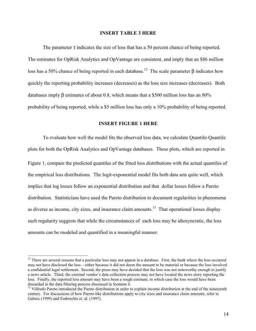
The parameter τ indicates the size of loss that has a 50 percent chance of being reported.

The estimates for OpRisk Analytics and OpVantage are consistent, and imply that an $86 million

loss has a 50% chance of being reported in each database.12 The scale parameter β indicates how

quickly the reporting probability increases (decreases) as the loss size increases (decreases). Both

databases imply β estimates of about 0.8, which means that a $500 million loss has an 80%

probability of being reported, while a $5 million loss has only a 10% probability of being reported.

INSERT FIGURE 1 HERE

To evaluate how well the model fits the observed loss data, we calculate Quantile-Quantile

plots for both the OpRisk Analytics and OpVantage databases. These plots, which are reported in

Figure 1, compare the predicted quantiles of the fitted loss distributions with the actual quantiles of

the empirical loss distributions. The logit-exponential model fits both data sets quite well, which

implies that log losses follow an exponential distribution and that dollar losses follow a Pareto

distribution. Statisticians have used the Pareto distribution to document regularities in phenomena

as diverse as income, city sizes, and insurance claim amounts.13 That operational losses display

such regularity suggests that while the circumstances of each loss may be idiosyncratic, the loss

amounts can be modeled and quantified in a meaningful manner.

12 There are several reasons that a particular loss may not appear in a database. First, the bank where the loss occurredmay not have disclosed the loss – either because it did not deem the amount to be material or because the loss involveda confidential legal settlement. Second, the press may have decided that the loss was not noteworthy enough to justifya news article. Third, the external vendor’s data collection process may not have located the news story reporting theloss. Finally, the reported loss amount may have been a rough estimate, in which case the loss would have beendiscarded in the data filtering process discussed in footnote 6.13 Vilfredo Pareto introduced the Pareto distribution in order to explain income distribution at the end of the nineteenthcentury. For discussions of how Pareto-like distributions apply to city sizes and insurance claim amounts, refer toGabaix (1999) and Embrechts et. al. (1997).

15

The fit of both Quantile-Quantile plots does deteriorate towards the tail of the loss

distribution. The deterioration is more pronounced for the OpRisk data, for which the largest

reported loss of about $3 billion (or e8 in the figure) significantly exceeds the largest loss predicted

loss of $1.8 billion (e7.5 in the figure). One possible reason for this deterioration is that $1 million

is too low a threshold for the POT approach, so that the GPD approximation does not fully capture

the tail behavior of losses. We will revisit the issue of whether $1 million is a high enough

threshold towards the end of this section.

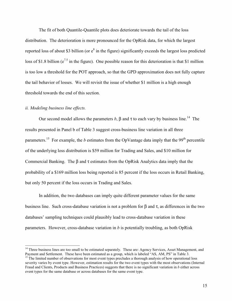
ii. Modeling business line effects.

Our second model allows the parameters b, β and τ to each vary by business line.14 The

results presented in Panel b of Table 3 suggest cross-business line variation in all three

parameters.15 For example, the b estimates from the OpVantage data imply that the 99th percentile

of the underlying loss distribution is $59 million for Trading and Sales, and $10 million for

Commercial Banking. The β and τ estimates from the OpRisk Analytics data imply that the

probability of a $169 million loss being reported is 85 percent if the loss occurs in Retail Banking,

but only 50 percent if the loss occurs in Trading and Sales.

In addition, the two databases can imply quite different parameter values for the same

business line. Such cross-database variation is not a problem for β and τ, as differences in the two

databases’ sampling techniques could plausibly lead to cross-database variation in these

parameters. However, cross-database variation in b is potentially troubling, as both OpRisk

14 Three business lines are too small to be estimated separately. These are: Agency Services, Asset Management, andPayment and Settlement. These have been estimated as a group, which is labeled “AS, AM, PS” in Table 3.15 The limited number of observations for most event types precludes a thorough analysis of how operational lossseverity varies by event type. However, estimation results for the two event types with the most observations (InternalFraud and Clients, Products and Business Practices) suggests that there is no significant variation in b either acrossevent types for the same database or across databases for the same event type.

16

Analytics and OpVantage should be sampling from the same underlying loss distribution. It is thus

important to determine whether the cross-business line parameter variation is statistically

significant. To do so, we note that model 1 is a restricted version of model 2, and perform a

likelihood ratio test in the usual manner. We find that the test statistic exceeds the 1% critical

value, which indicates that the cross-business line variation in the observed loss distribution is

statistically significant.

We now consider whether cross-business line variation in the observed loss distribution

derives from variation in the underlying loss distribution or from variation in the distribution of the

unobserved truncation variable (or both). To do so, we first estimate model 3, in which b is held

constant across business lines but β and τ remain unrestricted. The results are presented in Panel c

of Table 3. Because model 3 is a restricted version of model 2, we can again use a likelihood ratio

test to evaluate the hypothesis that b is constant across business lines. For both databases, the test

statistics are less than the 5% critical value. Thus, we cannot reject the null that b is constant

across business lines. Next, we estimate model 4, a restricted version of model 2 in which β and τ

are held constant across business lines (but b is unrestricted). The results are presented in Panel d

of Table 3. Here also, the likelihood test statistics for both databases are less than the 5% critical

value. Thus, we cannot reject the null hypothesis that β and τ are constant across business lines.

To summarize, we have found that while there is statistically significant cross-business line

variation in the observed loss distribution, we cannot definitively attribute this finding to either

variation in the severity parameter b or variation in the truncation parameters β and τ. We note,

however, that the results for models 3 and 4 do resolve the issue of cross-database parameter

variation. Panels c and d of Table 3 show that the parameter estimates for each of these models are

17

remarkably consistent across the two external databases, which suggests that the cross-database

variation in the results for model 2 may be attributed to estimation error.

iii. Robustness.

The results presented in Table 3 were derived using a Peaks Over Threshold methodology, in

which losses exceeding a high threshold are assumed to follow a Generalized Pareto Distribution.

It is well known that POT can be highly sensitive to the choice of threshold. Because the GPD is

only an approximation, it is possible that the parameter estimates resulting from one threshold

could differ substantially from those resulting from another even higher threshold for which the

GPD is a better approximation.

INSERT TABLE 4 HERE

To check the sensitivity of our results to threshold selection, we re-estimate the models using

various thresholds between $2 million and $10 million. The results for Model 1 are reported in

Table 4.16 Although the point estimates for b do vary somewhat according to the threshold, this

variation does not appear statistically significant. Furthermore, there is no trend in the estimates as

the threshold increases. Thus, the results suggest that the parameter estimates based on the original

$1 million threshold are robust with respect to threshold selection.

In section six, we will consider the implications of our findings for the level of capital that

large internationally active banks might be expected to hold. To do so, we assume that the loss

data underlying our results are representative of the risks to which these institutions are currently

exposed. In results not reported, we performed a preliminary validation of these assumptions. The

external databases report several measures of bank size (e.g., assets, revenue, number of

16 For the sake of compactness, we present these results only for model 1. The results for models 2 to 4 are similar.

18

employees). For each of these measures, we split the sample into banks below the median size and

banks above the median size. We found no statistically significant relationship between the size of

a bank and the value of the tail thickness parameter b. We also found no evidence of any

significant time trend in b.

We conclude this section with a summary of the more notable empirical results. Overall,

the results based on U.S. data indicate that the logit-GPD model provides a good estimate of the

severity of the loss data in external databases. In addition, the estimated loss severity is quite

similar for the two databases examined. The observed loss distribution does vary by business line,

but it is not clear whether this variation is a feature of the underlying losses or of the unobserved

truncation variable. Finally, correcting the external data for reporting biases is important, and

significantly decreases the estimated loss severity.

VI. Simulation results

This section considers the implications of our findings for regulatory capital at large

internationally active banks. The empirical work in the previous sections focuses on the severity of

large operational losses. However, capital requirements also depend on how frequently these

losses are likely to occur. We base our capital analysis on the simple and commonly-made

assumption that the frequency of large losses follows a Poisson distribution. The Poisson

assumption implies that the probability of a loss occurring does not depend on the time elapsed

since the last loss, so that loss events tend to be evenly spaced over time.17

17 Some have suggested that the frequency of large operational losses does vary over time (Danielsson et. al., 2001;Embrechts and Samorodnitsky, 2002). In this case, the Poisson assumption is not technically correct. However, webelieve that time-variation in the loss arrival rate should result in a fatter-tailed aggregate loss distribution, so that ourcurrent capital estimates would be conservative. A rigorous investigation of this issue is left to future research.

19

Our discussions with banks suggest that a typical large internationally active bank

experiences an average of 50 to 80 losses above $1 million per year. Smaller banks and banks

specializing in less risky business lines may encounter significantly fewer losses in excess of $1

million, and extremely large banks weighted towards more risky business lines could encounter

more large losses. The frequency of large losses may also depend on the control environment at an

individual institution. We thus consider a wide range of values for the Poisson parameter λ of

between 30 and 100 losses in excess of $1 million per year.

We assume that the severity of losses exceeding $1 million follows the log-exponential

distribution that was estimated in previous sections, with values for the b parameter of 0.55, 0.65

and 0.75. These values provide a reasonable range around our estimates based on bank-wide

losses.18 This range also captures the possibility that the severity of large losses at a particular bank

may depend on that bank’s control environment.

INSERT TABLE 5 HERE

Using the above range of frequency and severity assumptions, we simulate one million

years’ experience of losses exceeding $1 million. The results are presented in Table 5. Panel a

presents the results for the 99.9 percent confidence level used by many banks. The capital for a

bank with 60 events a year would range from $600 million for a b estimate of 0.55 to $4.0 billion

for a b estimate of 0.75. For a bank with 80 events a year, the range increases to $700 million to

$4.9 billion. For a very large bank with a poor control environment, 100 loss events with a b of

0.75 would result in capital of $6 billion.

18 Our results for model 4 suggest that the loss severity distribution may vary by business line. However, our currentfocus is on bank-wide risk capital at a large bank with a typical mix of business lines. Thus, we focus on those bestimates that apply to all business lines (models 1 and 3). Capital estimates for a bank specializing in one or twobusiness lines may differ from those reported in Table 5.

20

Panel b reports the effect of increasing the soundness standard to the 99.97 percent

confidence level favored by some banks. The resulting increase in capital is much greater under

the heavy-tailed loss distribution than it would be under a lighter-tailed distribution such as the

Lognormal. For the previous example of a large bank with a poor control environment, capital

more than doubles to $14.4 billion.19

VII. Conclusion

Despite the many headline-grabbing operational losses that have occurred over the past

decade, banks have made limited progress in quantifying their exposure to operational risk.

Instead, operational risk management has emphasized qualitative approaches, such as enhancing

the firm’s control environment and monitoring so-called “key risk” indicators. This qualitative

emphasis has been driven in part by the lack of reliable operational loss data, and in part by the

belief that the idiosyncrasies of large operational losses would make modeling operational risk

exceedingly difficult even with reliable data.

This paper analyzes recently available databases of publicly disclosed operational losses.

We find that because large losses are more often disclosed than small losses, these databases have a

significant and unavoidable reporting bias. After correcting for this bias, however, we obtain

robust and realistic estimates of operational risk. Our estimates are consistent with the level of

capital some large financial institutions are currently allocating for operational risk, falling in the

range of $2-$7 billion.20 Furthermore, we find that the operational losses reported by major banks

display a surprising degree of statistical regularity, and that large losses are well modeled by the

same Pareto-type distribution seen in phenomena as disparate as city sizes, income distributions

19 An important caveat to this analysis is that external databases contain only losses exceeding $1 million in nominalvalue. Thus, we are not simulating the capital needed for smaller, more frequent losses.20 See footnote 1.

21

and insurance claim amounts. This regularity suggests that while the details and chronologies of

the loss events may be idiosyncratic, the loss amounts themselves can be modeled and quantified in

a meaningful manner.

Some have suggested that even if it is possible to measure operational risk, the benefits of

doing so may be outweighed by costs arising from the necessary investments in personnel and data

infrastructure. However, we find that operational risk will often exceed market risk, an area in

which banks have already made sizeable investments.21 As institutions increasingly rely on

sophisticated risk models to aid them during important strategic and business decision-making

processes, it will become increasingly important for them to incorporate appropriately the

quantification of operational risk. The failure to do so could seriously distort RAROC models,

compensation models, economic capital models, and investment models frequently used by

financial institutions.

The extent to which operational risk should inform strategic decisions (e.g., which business

lines to grow) ultimately depends on how much this risk can vary within a firm. Our analysis of

whether the underlying loss distribution varies across business lines was inconclusive, but it is

possible that the cross-business line results will become clearer as the vendors expand and improve

their databases. The amount of intra-firm variation in operational risk also depends on the answers

to two open questions. First, to what extent does the frequency distribution of large losses vary

across business lines? Second, are there dimensions other than business line that might be

associated with intra-firm variation in operational risk? Clearly, the magnitude of our estimates

suggests that any intra-firm variation in operational risk is likely to be large. Thus, answering these

two questions is an important area for future research.

21 See footnote 2.

22

Another open question is how a bank’s risk control environment affects the severity

distribution of large operational losses. Because the external databases include losses experienced

by a wide range of financial institutions, our severity estimates should apply to the “typical” large

internationally active bank. Banks with better than average risk controls may have a thinner-tailed

severity distribution, which would reduce the likelihood of very large losses. Similarly, banks with

worse than average controls may have an increased exposure to large losses. Thus, a risk manager

would need to adjust for the control environment at her institution before applying our results and

techniques. Determining how to make such adjustments is another important area for future

research.

Although much remains to be done, our findings do have several implications that are of

immediate practical relevance. First, our analysis indicates that reporting biases in external data are

significant, and can vary by both business line and loss type. Failure to account for these biases

will tend to overstate the amount of operational risk that a bank faces, and could also distort the

relative riskiness of various business lines. More generally, the analysis indicates that external data

can be an important supplement to banks’ internal data. While many banks should have adequate

data for modeling high frequency low severity operational losses, few will have sufficient internal

data to estimate the tail properties of the very largest losses. Our results show that using external

data is a feasible solution for understanding the distribution of these large losses.

23

References

Amemiya, Takeshi, 1984, Tobit models: a survey, Journal of Econometrics 24, 3-63.

Basel Committee on Banking Supervision, 1996, Amendment to the Capital Accord to IncorporateMarket Risks.

Baud, Nicolas, Antoine Frachot and Thierry Roncalli, 2002, Internal data, external data andconsortium data for operational risk measurement: How to pool data properly?, Working paper,Groupe de Recherche Opérationelle, Crédit Lyonnais.

Berkowitz, Jeremy and James O'Brien, 2002, How accurate are Value-at-Risk models atcommercial banks?, Journal of Finance 58, 1093-1111.

Carey, Mark, 1998, Credit risk in private debt portfolios, Journal of Finance 53, 1363-1387.

Catarineu-Rabell, Eva, Patricia Jackson and Dimitrios Tsomocos, 2002, Procyclicality and the newBasel accord – banks’ choice of loan rating system, Working paper, Bank of England.

Coles, Stuart, 2001, An Introduction to Statistical Modeling of Extreme Values (Springer-Verlag,London).

Daníelsson, Jon, Paul Embrechts, Charles Goodhart, Con Keating, Felix Muennich, Olivier Renaultand Hyun Shin, 2001, An academic response to Basel II, Special paper No. 130, Financial marketsGroup, London School of Economics.

Danielsson, Jon, Laurens de Haan, Liang Peng and Casper de Vries, 2000, Using a bootstrapmethod to choose the sample fraction in tail index estimation, Journal of Multivariate Analysis 76,226-248.

Embrechts, Paul and Gennady Samorodnitsky, 2002, Ruin theory revisited: Stochastic models foroperational risk, Working paper, ETH-Zurich and Cornell University.

Embrechts, Paul, Claudia Klüppelberg and Thomas Mikosch, 1997, Modelling Extremal Events forInsurance and Finance (Springer-Verlag, New York).

Gabaix, Xavier, 1999, Zipf’s Law for cities: an explanation, Quarterly Journal of Economics 114,739-767.

Greene, William, 1997, Econometric Analysis (Prentice Hall, Upper Saddle River, NJ).

Hendricks, Darryl, 1996, Evaluation of Value-at-Risk models using historical data, EconomicPolicy Review, Federal Reserve Bank of New York, 39-46.

Hirtle, Beverly, 2003, What market risk capital reporting tells us about bank risk, forthcoming inEconomic Policy Review, Federal Reserve Bank of New York.

24

James, Christopher. 1996. RAROC-based capital budgeting and performance evaluation: a casestudy of bank capital allocation, Working paper, University of Florida.

Maddala, G. S., 1983, Limited Dependent and Qualitative Variables in Econometrics (CambridgeUniversity Press, Cambridge).

Pictet, Olivier, Michel Dacorogna and Ulrich Muller, 1998, Hill, bootstrap and jackknife estimatorsfor heavy tails, in Murad Taqqu, ed.: A Practical Guide to Heavy Tails: Statistical Techniques forAnalyzing Heavy Tailed Distributions (Birkhauser, Boston).

Prisker, Matthew, 1997, Evaluating Value-at-Risk methodologies: Accuracy versus computationaltime, Journal of Financial Services Research 12, 201-242.

Table 1. Descriptive Statistics by Basel Business Line.A "-" indicates that there were too few observations for the quantile to be reported.

Panel a. Losses that occurred in the U.S.

Business Line 50% 75% 95% 50% 75% 95%Corporate Finance 6% 6 23 - 4% 8 23 - Trading & Sales 9% 10 44 334 9% 10 27 265 Retail Banking 38% 5 11 52 39% 5 12 60 Commercial Banking 21% 7 24 104 16% 8 28 123 Payment & Settlement 1% 4 11 - 1% 4 11 - Agency Services 2% 22 110 - 3% 9 28 - Asset Management 5% 8 20 - 6% 8 22 165 Retail Brokerage 17% 4 12 57 22% 4 13 67 Total 100% 6 17 88 100% 6 17 93

Panel b. Losses that occurred outside the U.S.

Business Line 50% 75% 95% 50% 75% 95%Corporate Finance 2% 13 - - 3% 12 27 - Trading & Sales 9% 30 125 - 12% 25 66 - Retail Banking 41% 6 27 101 44% 9 29 272 Commercial Banking 30% 15 42 437 21% 35 91 323 Payment & Settlement 1% 5 - - 1% 13 - - Agency Services 2% 45 - - 3% 20 77 - Asset Management 3% 5 47 - 5% 7 23 - Retail Brokerage 12% 10 42 - 11% 8 34 - Total 100% 10 36 221 100% 13 46 288

Percentiles ($M) Percentiles ($M)OpRisk Analytics OpVantage

% of All Losses

% of All Losses

OpRisk Analytics OpVantage Percentiles ($M) Percentiles ($M)% of All

Losses% of All

Losses

Table 2. Descriptive Statistics by Basel Event TypeA "-" indicates that there were too few observations for the quantile to be reported.

Panel a. Losses that occurred in the U.S.

Event Type 50% 75% 95% 50% 75% 95%Internal Fraud 23.0% 4 10 42 27.0% 6 16 110 External Fraud 16.5% 5 17 93 16.6% 4 12 70 EPWS 3.0% 4 14 - 3.3% 5 11 - CPBP 55.5% 7 20 95 48.1% 7 20 99 Damage Phys. Assets 0.4% 18 - - 0.3% 20 - - BDSF 0.2% 36 - - 0.4% 10 - - EDPM 1.3% 9 27 - 4.2% 4 11 - Total 100.0% 6 17 88 100.0% 6 17 93

Panel b. Losses that occurred outside the U.S.

Event Type 50% 75% 95% 50% 75% 95%Internal Fraud 48.5% 9 35 259 42.9% 15 62 381 External Fraud 15.3% 7 27 - 21.6% 10 28 136 EPWS 0.8% 7 - - 1.6% 2 7 - CPBP 32.6% 14 51 374 28.6% 13 51 359 Damage Phys. Assets 0.0% - - - 0.3% 163 - - BDSF 0.8% 7 - - 0.5% 3 - - EDPM 1.9% 29 - - 4.6% 5 19 - Total 100.0% 10 36 221 100.0% 13 46 288

OpRisk Analytics OpVantage Percentiles ($M) Percentiles ($M)% of All

Losses% of All

Losses

Percentiles ($M) Percentiles ($M)OpRisk Analytics OpVantage

% of All Losses

% of All Losses

Table 3. Estimation results by Basel Business Line - US Losses Only.

Panel a. Models 1 and 2. Model 1 Model 2

All BL's

Corporate Finance

Trading& Sales

Retail Banking

Cmcl. Banking

AS, AM, PS

Retail Brok.

OpRisk Analytics Estimates:Exponential: b 0.64 0.72 0.68 0.73 0.52 0.61 0.78

(0.08) (0.31) (0.20) (0.20) (0.16) (0.63) (0.22)Intensity of choice: β 0.78 0.76 0.76 0.75 0.59 0.66 1.05

(0.10) (0.26) (0.22) (0.09) (0.20) (0.59) (0.30)Threshold: τ 4.45 3.98 5.13 2.81 4.78 4.67 3.68

(0.36) (1.27) (0.77) (1.23) (0.53) (2.40) (1.41)Emp. 99th Percentile, $M 302 278 709 186 283 297 261Est. 99th Percentile, $M 19 27 23 28 11 17 36exp(τ), $M 86 54 169 17 119 107 40

OpVantage Estimates:Exponential: b 0.66 0.84 0.89 0.62 0.49 0.79 0.58

(0.07) (0.25) (0.23) (0.11) (0.13) (0.27) (0.13)Intensity of choice: β 0.82 0.60 0.91 0.83 0.54 0.86 0.76

(0.09) (0.11) (0.17) (0.17) (0.14) (0.21) (0.20)Threshold: τ 4.46 2.64 4.14 4.27 4.82 4.16 4.43

(0.32) (0.83) (1.54) (0.57) (0.40) (1.33) (0.54)Emp. 99th Percentile, $M 388 326 591 203 332 400 188Est. 99th Percentile, $M 21 48 59 18 10 39 15exp(τ), $M 86 14 63 72 124 64 84

Model 1 restricts each parameter to be equal across business lines, Model 2 places no parameter restrictions across business lines, Model 3 restricts b to be equal across business lines, and Model 4 restricts β and τ to be equal across business lines. Parentheses denote standard errors for parameter estimates. Losses in the Agency Services, Asset Management, and Payment and Settlement business lines have been grouped together for estimation purposes. Results for these business lines are reported in the column labeled “AS, AM, PS.”

Table 3. Estimation results by Basel Business Line - US Losses Only.

Panel b. Model 3.

AllCorporate

FinanceTrading& Sales

Retail Banking

Cmcl. Banking

AS, AM, PS

Retail Brok.

OpRisk Analytics Estimates:Exponential: b 0.62

(0.08)Intensity of choice: β 0.67 0.69 0.77 0.71 0.67 0.83

(0.10) (0.10) (0.10) (0.10) (0.09) (0.14)Threshold: τ 4.31 5.29 3.75 4.50 4.64 4.46

(0.65) (0.63) (0.48) (0.43) (0.61) (0.82)exp(τ), $M 74 198 43 90 104 86

OpVantage Estimates:Exponential: b 0.64

(0.07)Intensity of choice: β 0.54 0.71 0.85 0.68 0.72 0.83

(0.07) (0.08) (0.11) 0.08 (0.08) (0.11)Threshold: τ 3.24 5.23 4.22 4.48 4.86 4.28

(0.46) (0.64) (0.47) (0.35) (0.58) (0.49)exp(τ), $M 26 187 68 88 129 72

Model 1 restricts each parameter to be equal across business lines, Model 2 places no parameter restrictions across business lines, Model 3 restricts b to be equal across business lines, and Model 4 restricts β and τ to be equal across business lines. Parentheses denote standard errors for parameter estimates. Losses in the Agency Services, Asset Management, and Payment and Settlement business lines have been grouped together for estimation purposes. Results for these business lines are reported in the column labeled “AS, AM, PS.”

Table 3. Estimation results by Basel Business Line - US Losses Only.

Panel c. Model 4.

AllCorporate

FinanceTrading& Sales

Retail Banking

Cmcl. Banking

AS, AM, PS

Retail Brok.

OpRisk Analytics Estimates:Exponential: b 0.68 0.74 0.57 0.65 0.70 0.58

(0.09) (0.11) (0.06) (0.08) (0.10) (0.07)Intensity of choice: β 0.74

(0.09)Threshold: τ 4.36

(0.33)exp(τ), $M 78

OpVantage Estimates:Exponential: b 0.72 0.76 0.59 0.72 0.72 0.60

(0.08) (0.09) (0.05) (0.08) (0.08) (0.05)Intensity of choice: β 0.78

(0.07)Threshold: τ 4.31

(0.28)exp(τ), $M 74

Model 1 restricts each parameter to be equal across business lines, Model 2 places no parameter restrictions across business lines, Model 3 restricts b to be equal across business lines, and Model 4 restricts β and τ to be equal across business lines. Parentheses denote standard errors for parameter estimates. Losses in the Agency Services, Asset Management, and Payment and Settlement business lines have been grouped together for estimation purposes. Results for these business lines are reported in the column labeled “AS, AM, PS.”

Table 4. Estimation results for various POT threshold values.

Threshold value u.$1M $2M $3M $5M $10M

OpRisk Analytics Estimates:Exponential: b 0.64 0.69 0.66 0.64 0.70

(0.08) (0.10) (0.10) (0.11) (0.12)Intensity of choice: β 0.78 0.81 0.81 0.82 0.73

(0.10) (0.09) (0.11) (0.13) (0.12)Threshold: τ 4.45 4.10 4.30 4.55 3.86

(0.36) (0.50) (0.56) (0.71) (0.83)

OpVantage Estimates:Exponential: b 0.66 0.77 0.80 0.70 0.68

(0.07) (0.08) (0.09) (0.11) (0.18)0.82 0.85 0.84 0.89 0.91

(0.09) (0.06) (0.06) (0.10) (0.12)4.46 3.69 3.46 4.34 4.52

(0.32) (0.45) (0.56) (0.81) (1.56)

The following table presents parameter estimates for Model 1 as the threshold u is increased from $1 million to $10 million. For example, a $10 million threshold indicates that only losses exceeding $10 million were included in the analysis. Parentheses denote standard errors.

Table 5. Percentiles (in $ Billions) of simulated aggregate loss distributions.

Panel a. Capital estimates (in $Billions) at the 99.9 percent confidence level.

30 40 50 60 70 80 90 1000.55 0.4 0.4 0.5 0.6 0.6 0.7 0.7 0.80.65 0.9 1.1 1.3 1.4 1.6 1.8 1.9 2.10.75 2.4 3.1 3.6 4.0 4.5 4.9 5.3 6.0

Panel b. Capital estimates (in $Billions) at the 99.97 percent confidence level.

30 40 50 60 70 80 90 1000.55 0.6 0.8 0.8 1.0 1.1 1.2 1.2 1.30.65 1.8 2.2 2.5 2.7 3.2 3.5 3.8 4.00.75 5.8 7.3 7.7 10.0 10.6 12.0 12.7 14.4

This table reports the 99.9th and 99.97th percentiles from simulated aggregate loss distributions. We assumed for these simulations that the severity of operational losses exceeding $1 million followed a log-exponential distribution with mean b , and that the frequency of these losses followed a Poisson distribution with mean λ. The percentiles are reported in billions of dollars, and can be interpreted as estimates of economic capital under the aforementioned distributional assumptions.

Note. The above figures estimate the capital required to cover operational losses exceeding $1 Million. Additional capital is required to cover losses below $1 Million.

Exponential parameter, b .

Average Number of Losses Exceeding $1 Million per Year

Exponential parameter, b .

Average Number of Losses Exceeding $1 Million per Year

Figure 1. Quantile-Quantile plots for Model 1.

Panel a. OpRisk Analytics data, all business lines, U.S. losses only.

0

1

2

3

4

5

6

7

8

9

0 1 2 3 4 5 6 7 8 9

Fitted Quantile, log($M)

Empi

rical

Qua

ntile

, log

($M

)

Panel b. OpVantage data, all business lines, U.S. losses only.

0

1

2

3

4

5

6

7

8

9

0 1 2 3 4 5 6 7 8 9

Fitted Quantile, log($M)

Empi

rical

Qua

ntile

, log

($M

)