using hyperbolic systems of balance laws for modeling ... · using hyperbolic systems of balance...
TRANSCRIPT
Using hyperbolic systems of balance laws
for modeling, control and stability analysis
of physical networks
Lecture notes for the Pre-Congress Workshop on Complex Embedded and Networked Control Systems
17th IFAC World Congress, Seoul, Korea.
July 5-6, 2008
G. Bastin1, J-M. Coron2 and B. d’Andrea-Novel3
Abstract
The operation of many physical networks having an engineering relevance may be repre-sented by hyperbolic systems of balance laws in one space dimension. By using a Lyapunovstability analysis, it can be shown that the exponential stability of the equilibrium is guaran-teed if the boundary conditions are dissipative. This essential property is helpful for solvingthe associated control problem of designing control laws at the network junctions in order tostabilize the system. This control design issue is illustrated with an application to water levelcontrol in hydraulic networks.
1Center for Systems Engineering and Applied Mechanics (CESAME), Department of Mathematical En-gineering, Universite catholique de Louvain, 4, avenue G. Lemaıtre, 1348 Louvain-la-Neuve, [email protected]
2Laboratoire Jacques-Louis Lions, Department of Mathematics, Universite Paris-VI, Boite 187, 75252 ParisCedex 05, France. [email protected]
3Centre de Robotique (CAOR), Ecole Nationale Superieure des Mines de Paris, 60, Boulevard Saint Michel,75272 Paris Cedex 06, France. [email protected]
1

1. Introduction.
The operation of many physical networks having an engineering relevance may be representedby hyperbolic systems of balance laws in one space dimension. Among the potential applicationswe have in mind, we mention for instance hydraulic networks (for irrigation or navigation), electricline networks, road traffic networks or gas pipeline networks.
In each of these applications, the network is represented by a directed graph with edges andnodes. Along the edges, the dynamics of the concerned physical quantities are modelled by hyper-bolic partial differential equations (PDEs) under the form of so-called 2×2 systems of balance laws.The nodes of the graph represent the physical junctions between some of the edges of the network.The mechanisms occuring at these junctions are modelled by algebraic relations that determinethe boundary conditions of the PDEs. They generally depend on network physical constraints but,in many instances, they can also be assigned by using appropriate control devices (like hydraulicgates in open channels or traffic lights in road networks).
In this paper, our main concern is to discuss the exponential stability of the classical solutionsfor such physical network systems. The analysis relies on Lyapunov functions. Essentially, weshall see that the time derivative of the Lyapunov function can be made negative if the boundaryconditions are dissipative. There is therefore an underlying control problem which is the problemof designing the control laws at the network junctions in order to make the corresponding boundaryconditions dissipative.
The content of the paper is summarized as follows.In Section 2 we give the basic definition of an hyperbolic 2×2 system of balance laws over a
finite space interval.In Section 3 we give three physical examples of such systems : the telegrapher equations for
electrical lines, the Saint-Venant equations for hydraulic channels, the Aw-Rascle equations forroad traffic.
In section 4, we give the general equations of networks represented by a set of n hyperbolic2×2 systems of balance laws.
In section 5, the purpose is to present the characteristic form of hyperbolic 2×2 systems ofbalance laws and its linearisation with respect to a steady-state equlibrium.
In Section 6, we present a Lyapunov function used for analysing the asymptotic convergenceof the classical solutions of the linearised system under linear boundary conditions. This analysisleads to the concept of dissipative boundary conditions that guarantee the exponential stability ofthe system.
In Section 7, we present an explicit characterisation of sufficient dissipative boundary conditionswhich guarantee the system exponential stability in the case where the considered balance lawsare almost conservative.
In Section 8, it is shown that, for hydraulic networks described by Saint-Venant equations, thedissipative boundary conditions may be sufficient to guarantee the stability for systems of balancelaws which deviate widely from their corresponding conservation laws.
In Section 9, we address the implications of the previous stability properties for the design ofboundary feedback control for physical networks when the boundary conditions are assigned bycontrol devices that are used for network regulation and stabilisation.The particular example ofthe level control problem in hydraulic networks is treated in details.
In Section 10, we explain how the linear Lyapunov stability analysis developed in the previoussections can be extended to the case of nonlinear hyperbolic systems of balance laws.
Finally, in Section 11, we conclude the paper with bibliographical notes for the readers whowould like to go deeper in the subject.
2
2. Hyperbolic 2×2 systems of balance laws.
In this section we give the basic definition of an hyperbolic 2×2 system of balance laws overa finite space interval as it will be used throughout the paper. Let Ω be a non-empty connectedopen set in R2. A 2×2 system of balance laws is a system of PDEs of the form
∂ty + ∂xf(y) + g(y) = 0 t ∈ [0,+∞) x ∈ [0, L] (1)
where
• t and x are the two independent variables: a time variable t ∈ [0,+∞) and a space variablex ∈ [0, L] over a finite interval;
• y , (y1 y2)T : [0,+∞) × [0, L] → Ω is the vector of the two dependent variables calleddensities;
• f ∈ C1(Ω,R2) is the vector of the flux densities;
• g ∈ C1(Ω,R2) is the vector of source terms.
Since f is a C1 function, system (1) can be written under the form of a quasi-linear system ofPDEs
∂ty + A(y)∂xy + g(y) = 0
with the jacobian matrix A(y) , ∂f/∂y. The system (1) is strictly hyperbolic if A(y) has twodistinct real eigenvalues a1(y) 6= a2(y) ∀y ∈ Ω.
In the special case where there are no source terms (i.e. g(y) = 0 ∀y∈ Ω), the system (1)reduces to
∂ty + ∂xf(y) = 0 (2)
which constitutes a so-called hyperbolic 2×2 system of conservation laws.
3. Examples.
In this section we shall give three physical examples of such systems. The first example is thewell-known telegrapher equation for the modelling of electric lines. It is a very simple linear system.The two other examples are nonlinear. They are presented here because they are particularly wellsuited for illustrating the theoretical developments of the paper : the first one is the well-knownSaint-Venant equation for modelling the water flow in open channels [9]; the second one is theAw-Rascle equation for modelling the road traffic flow [1].
The telegrapher equation
This equation, which is a simplification of the Maxwell equations, describes the propagationof an electric signal along an electrical line with inductance L, capacitance C, resistance R andadmittance G under the form of a 2×2 system of balance laws
∂t
(IV
)+ ∂x
(−L−1V−C−1I
)+(
RL−1IGC−1V
)= 0
3
with I(t, x) the current and V (t, x) the voltage at time t and location x along the line. From thisequation, we have
y =(
IV
)A(y) =
(0 −L−1
−C−1 0
)g(y) =
(RL−1IGC−1V
).
The system is hyperbolic since the matrix A has two distinct real eigenvalues a1,2 = ±(√LC)−1.
The Saint-Venant equation
This equation, which is a simplification of the Navier-Stokes equation, describes the waterpropagation in a prismatic channel with rectangular cross-section and constant slope as follows :
∂t
(HV
)+ ∂x
(HV
12V
2 + gH
)+(
0g[CV 2H−1 − S]
)= 0 (3)
with H(t, x) the water height and V (t, x) the water velocity at time t and location x along thechannel. g is the gravity constant, C a friction parameter and S the canal slope. From this equationwe have :
y =(HV
)A(y) =
(V Hg V
)g(y) =
(0
g[CV 2H−1 − S]
).
The eigenvalues of the matrix A(y) are :
a1(y) = V +√gH and a2(y) = V −
√gH.
The system is hyperbolic when the so-called Froude’s number Fr = V/√gH < 1. In such a case,
the flow in the channel is said to be fluvial or subcritical.
The Aw-Rascle equation
The Aw-Rascle equation is a basic fluid model for the description of road traffic dynamics. Itis directly given here in the quasi-linear form. The model is as follows:
∂t
(ρV
)+(V ρ0 V + ρV ′o(ρ)
)∂x
(ρV
)+
(0
V − Vo(ρ)τ
)= 0 (4)
with ρ(t, x) the traffic density and V (t, x) the speed of the vehicles at time t and location x alongthe road. The function Vo(ρ) is the preferential speed function : it is a decreasing function thatrepresents the relation, in the average, beween the speed of the vehicles and the traffic density (thehigher the density, the lower the speed of the vehicles). The constant parameter τ is a positivetime constant. The eigenvalues of the matrix A(y) are :
a1(y) = V and a2(y) = V + ρV ′o(ρ).
The system is hyperbolic.
4

4. Networks of hyperbolic 2×2 systems of balance laws.
We now consider physical networks (e.g. irrigation or road networks). We assume that thetopology of the network is represented by a graph. The edges of the graph represent the physicallinks (i.e the canals or the roads) having dynamics expressed by n hyperbolic 2×2 systems ofbalance laws
∂tyi + Ai(yi)∂xyi + gi(yi) = 0 i = 1, . . . , n with yi ,
(yiyn+i
)(5)
or in a compact matrix form∂tY + F(Y)∂xY + G(Y) = 0 (6)
with the notation Y , (y1, y2, . . . , yn, yn+1, . . . , y2n)T and the maps F and G defined accordingly.The nodes of the graph represent the physical junctions between the links of the network. The
physical interconnection mechanisms that occur at the junctions are supposed to be described bya set of static ”junction models” that fix the boundary conditions of the PDEs (5). At this stage,it is not necessary to give a more precise formulation of these junction models. The issue will beaddressed in Section 9.
5. Steady-state, characteristic form and linearisation.
The main purpose of this section is to present the so-called characteristic form of hyperbolic2×2 systems of balance laws and its linearisation with respect to a steady-state equlibrium.
Steady-state : A steady-state solution (or equilibrium) for each system (5) is a constant solutionyi(t, x) = y∗i ∀t ∈ [0,+∞), ∀x ∈ [0, L] which satisfies the condition gi(y∗i ) = 0.
It is a well known property (e.g. [11], [15]) that any system of the form (5) can be transformed intoa (diagonalised) characteristic form by using appropriate characteristic coordinates. This meansthat, for any equilibrium y∗i , there exists a change of coordinates ξi = Φi(yi) such that
1. Φi(y∗i ) = 0
2. the Jacobian matrix of Φi diagonalises the coefficient matrix Ai(yi) in Ω:
Φ′i(yi)Ai(yi) = Di(yi)Φ′i(yi) yi ∈ Ω with Di(yi) , diagai(yi), an+i(yi).
(ai(yi), an+i(yi) denote the two eigenvalues of the matrix Ai(yi)).
Finding the change of coordinates ξi(yi) requires to find a solution of the first order partialdifferential equation Φ′i(yi)Ai(yi) = Di(yi)Φ′i(yi). As it is shown by Lax in [11, pages 34-35], thispartial differential equation can be reduced to the integration of ordinary differential equations.Moreover, in many cases, these ordinary differential equations can be explicitly solved by usingseparation of variables, homogeneity or symmetry properties. Below we shall give the explicitsolutions for the Saint-Venant and the Aw-Rascle equations. See also [15, Tome I, pages 146-147,page 152] for other examples.
5

In the coordinates ξi , (ξi, ξn+i)T , each system (5) can then be rewritten in the characteristicform:
∂tξi + Ci(ξi)∂xξi + hi(ξi) = 0 (7)
with Ci(ξi) , Di(Φ−1i (ξi)) and hi(ξi) , Φ′i(Φ
−1i (ξi)gi(Φ−1
i (ξi)).
The network model (6) is then written in a more compact characteristic matrix form
∂tξ + C(ξ)∂xξ + h(ξ) = 0 (8)
with the notation ξ , (ξ1, ξ2, . . . , ξn, ξn+1, . . . , ξ2n) and the corresponding definitions for the mapsC and h:
C(ξ) , diagc1(ξ1, ξn+1), c2(ξ2, ξn+2), . . . , cn+1(ξ1, ξn+1), . . . , c2n(ξn, ξ2n)
h(ξ) = (h1(ξ1, ξn+1), h2(ξ2, ξn+2), . . . , hn+1(ξ1, ξn+1), . . . , h2n(ξn, ξ2n))T .
By definition of the coordinate transformation, the equilibrium of the characteristic form is zero(i.e. ξ∗i = Φi(y∗i ) = 0 ∀i). It follows that the linearised characteristic form about the equilibriumis the hyperbolic 2×2 system of linear balance laws given by
∂tξ + Λ∂xξ + Bξ = 0 with Λ , C(0) and B , h′(0). (9)
In the sequel, we shall use the notation Λ , diagλi, i = 1, . . . , 2n. The λi eigenvalues are calledcharacteristic velocities.
Examples
• For the Saint-Venant equation (3) an equilibrium is a constant state H∗, V ∗ that verifies therelation
SH∗ = C(V ∗)2.
The linearisation of the Saint-Venant equations around the equilibrium is given by equation(9) with the following characteristic state variables (ξ1, ξ2), characteristic velocities λ1, λ2
and matrix B:
ξ1 = (V − V ∗) + (H −H∗)√
g
H∗ξ2 = (V − V ∗)− (H −H∗)
√g
H∗
λ2 = V ∗ −√gH∗ < 0 < λ1 = V ∗ +
√gH∗
B ,
(γ δγ δ
)with γ =
gS
2( 2V ∗− 1√
gH∗
)> 0 and δ =
gS
2( 2V ∗
+1√gH∗
)> 0
• For the Aw-Rascle equation (4) an equilibrium is a constant state ρ∗, V ∗ that verifies therelation
V ∗ = Vo(ρ∗).
The linearisation of the Aw-Raxcle equation around the equilibrium is given by equation (9)with the following characteristic state variables (ξ1, ξ2), characteristic velocities λ1, λ2 andmatrix B:
ξ1 = V − V ∗ − V ′o(ρ∗)(ρ− ρ∗) ξ2 = V − V ∗
0 < λ2 = V ∗ + ρ∗V ′o(ρ∗) < λ1 = V ∗
B ,
(γ δγ δ
)with γ = −V
′o(ρ∗)τ
> 0 and δ =V ∗
τ> 0.
6
6. Lyapunov stability analysis of the linearised system.
In this section, we present a Lyapunov function which can be used for analysing the asymptoticconvergence of the classical solutions of the linearised system (9) under linear boundary conditionsof the general form
K0ξ(t, 0) + K1ξ(t, L) = 0, t ∈ [0,+∞) (10)
We consider the Cauchy problem
∂tξ + Λ∂xξ + Bξ = 0 t ∈ [0,+∞), x ∈ (0, L), (11a)K0ξ(t, 0) + K1ξ(t, L) = 0, t ∈ [0,+∞), (11b)ξ(0, x) = ξo(x), x ∈ (0, L). (11c)
This Cauchy problem is well-posed (see e.g. [5, Section 2.1 and Section 2.3]). This means thatfor any initial condition ξo ∈ L2((0, L); R2n) and for every T > 0, there exists C(T ) > 0 such thata solution ξ(t, x) ∈ C0([0,+∞);L2((0, 1); R2n)) exists, is unique and satisfies
‖ξ(t, ·)‖L2((0,1);R2n) 6 C(T )‖ξo‖L2((0,1);R2n), ∀t ∈ [0, T ].
Our concern is to analyse the exponential stability of the system (9)-(10) according to the followingdefinition.
Definition 1. The system (9)-(10) is exponentially stable (in L2-norm) if there exist ν > 0 andC > 0 such that, for every initial condition ξ0(x) ∈ L2((0, L); R2n) the solution to the Cauchyproblem (11) satisfies
‖ξ(t, ·)‖L2((0,L);R2n) 6 Ce−νt‖ξo‖L2((0,1);R2n).
The following candidate Lyapunov function is defined:
V =∫ L
0
ξTP(x)ξdx (12)
where the weighting matrix P(x) is defined as follows: P(x) , diagpie−σiµx, i = 1, . . . , 2n, withµ > 0, pi > 0 positive real numbers and σi = sign(λi).
The time derivative of V along the solutions of (11) is
V =∫ L
0
(∂tξ
TP(x)ξ + ξTP(x)∂tξ)dx
= −∫ L
0
(∂xξ
TΛP(x)ξ + ξTP(x)Λ∂xξ + ξTBTP(x)ξ + ξTP(x)Bξ)dx
= −∫ L
0
∂x(ξTM(x)ξ)dx−∫ L
0
ξT(BTP(x) + P(x)B
)ξ dx
with the positive diagonal matrix M(x) , diagpi|λi|e−σiµx, i = 1, . . . , 2n. Integrating by parts,
7

we obtain:
V = −∫ L
0
∂x
[ξTM(x)ξ
]dx−
∫ L
0
ξT(µM(x) + BTP(x) + P(x)B
)ξ dx
= −[ξTM(x)ξ
]L0−∫ L
0
ξT(µM(x) + BTP(x) + P(x)B
)ξ dx
= −[ξT (t, L)M(L)ξ(t, L)− ξT (t, 0)M(0)ξ(t, 0)
]−∫ L
0
ξT(µM(x) + BTP(x) + P(x)B
)ξ dx.
The system (9)-(10) is exponentially stable if this function V is negative definite. We have thusshown the following result.
Theorem 1. The system (9)-(10) is exponentially stable if there exist µ > 0 and pi > 0 i =1, . . . , 2n such that
C1. The boundary quadratic form ξT (t, 0)M(0)ξ(t, 0) − ξT (t, L)M(L)ξ(t, L) is positive definiteunder the constraint of the linear boundary condition K0ξ(t, 0) + K1ξ(t, L) = 0;
C2. The matrix µM(x) + BTP(x) + P(x)B is positive definite ∀x ∈ (0, L).
Boundary conditions that satisfy condition C1 are called Dissipative Boundary Conditions.Condition C1 is satisfied if and only if the leading principal minors of order > 4n of the matrix 0 K0 K1
−KT0 M(0) 0
−KT1 0 −M(L)
are strictly positive (see [18]).
7. Dissipative boundary conditions for systems of (almost) conservativelaws.
In this section, we will present a variant of Theorem 1 with an explicit characterisation of asufficient dissipative boundary condition which guarantees the system exponential stability in thecase where ‖B‖ is sufficiently small or, in more intuitive terms, when the considered balance lawsare almost conservative. We know that Λ is a diagonal matrix with non-zero real diagonal entries.Without loss of generality, possibly through a permutation of the state variables, we may assumethat
Λ = diagλ1, λ2, . . . , λ2n, λi > 0 ∀i ∈ 1, . . . ,m , λi < 0 ∀i ∈ m+ 1, . . . , 2n . (13)
We introduce the notations
ξ+ = (ξ1, . . . , ξm) and ξ− = (ξm+1, . . . , ξ2n) such that ξ = (ξ+T , ξ−T )
Λ+ = diagλ1, . . . , λm and Λ− = diag|λm+1|, . . . , |λ2n| such that Λ = diagΛ+,−Λ−.
With these notations, the linear hyperbolic system (9) is writtem
∂t
(ξ+
ξ−
)+(
Λ+ 00 −Λ−
)∂x
(ξ+
ξ−
)+ Bξ = 0. (14)
8

The general linear boundary condition (10) is written in the specific form(ξ+(t, 0)ξ−(t, L))
)=(K00 K01
K10 K11
)︸ ︷︷ ︸
(ξ+(t, L)ξ−(t, 0)
). (15)
K
Let Dp denote the set of diagonal p × p real matrices with strictly positive diagonal entries. Weintroduce the following norm for the matrix K:
ρ(K) , inf‖∆K∆−1‖,∆ ∈ D2n
where ‖ ‖ denotes the ususal matrix 2-norm. We have the following Theorem.
Theorem 2. If ρ(K) < 1, there exists ε > 0 such that, if ‖B‖ < ε, then the linear hyperbolicsystem (14)-(15) is exponentially stable.
Proof. With the above notations, the candidate Lyapunov function (12) is written
V =∫ L
0
[(ξ+TP0ξ
+)e−µx + (ξ−TP1ξ−)eµx
]dx. (16)
with P0 ∈ Dm, P1 ∈ D2n−m and µ > 0. The time derivative of V is
V = V1 + V2 (17)
with
V1 , −[ξ+TP0Λ+ξ+e−µx
]L0
+[ξ−TP1Λ−ξ−eµx
]L0
V2 ,∫ L
0
ξT(µP (x)Λ + BTP (x) + P (x)B
)ξ dx
and P (x) , diag P0e−µx, P1e
µx.
In order to prove that the boundary condition (15) is dissipative we will show that P0, P1 andµ can be selected such that V1 is a negative definite quadratic form. For this analysis, we introducethe following notations:
ξ−0 (t) , ξ−(t, 0) ξ+1 (t) , ξ+(t, L).
Using the boundary condition (15), we have
V1 = −[ξ+TP0Λ+ξ+e−µx
]L0
+[ξ−TP1Λ−ξ−eµx
]L0
= −(ξ+T
1 P0Λ+ξ+1 e−µL + ξ−T0 P1Λ−ξ−0
)+(ξ+T
1 KT00 + ξ−T0 KT
01
)P0Λ+
(K00ξ
+1 +K01ξ
−0
)+(ξ+T
1 KT10 + ξ−T0 KT
11
)P1Λ−
(K10ξ
+1 +K11ξ
−0
)eµL.
Since ρ(K) < 1 by assumption, there exist D0 ∈ Dm, D1 ∈ D2n−m and ∆ , diagD0, D1 suchthat
‖∆K∆−1‖ < 1. (18)
9

The matrices P0 and P1 are selected such that P0Λ+ = D20 and P1Λ− = D2
1. We define z0 , D0ξ−0 ,
z1 , D1ξ+1 and zT , (zT0 , z
T1 ). Then, using inequality (18), we have(
ξ+T1 KT
00 + ξ−T0 KT01
)P0Λ+
(K00ξ
+1 +K01ξ
−0
)+(ξ+T
1 KT10 + ξ−T0 KT
11
)P1Λ−
(K10ξ
+1 +K11ξ
−0
)= ‖∆K∆−1z‖2 < ‖z‖2 = ξ+T
1 P0Λ+ξ+1 + ξ−T0 P1Λ−ξ−0 .
It follows that µ can be taken sufficiently small such that V1 is a negative definite quadratic form.
Moreover, for any µ > 0, there exist clearly two positive constants ε > 0 and α > 0 such that
‖B‖ < ε ⇒ V2 6 −αV ⇒ V = V1 + V2 6 −αV.
Consequently the solutions of the system (14)-(15) exponentially converge to 0 in L2-norm.
8. Application to the linearised Saint-Venant equation.
In the previous section, we have shown that for systems with small ‖B‖, the dissipative bound-ary condition ρ(K) < 1 is a sufficient stability condition. However it must be emphasized that, inparticular instances, this stability condition may be valid even if ‖B‖ is not small. This is true inparticular for hydraulic networks described by Saint-Venant equations as long as the subcriticalflow condition is satisfied as we shall illustrate in the present section. For the sake of simplicity,we consider the specific case of a single pool of an open-channel, but the property can be eas-ily extended to networks of interconnected pools. As we have seen in Section 4, the linearisedSaint-Venant equation in characteristic form is written as
∂tξ1 + λ1∂xξ1 + γξ1 + δξ2 = 0 (19a)∂tξ2 − |λ2|∂xξ2 + γξ1 + δξ2 = 0 (19b)
with λ2 = V ∗ −√gH∗ < 0 < λ1 = V ∗ +
√gH∗
and γ =gS
2( 2V ∗− 1√
gH∗
)> 0 , δ =
gS
2( 2V ∗
+1√gH∗
)> 0.
We consider this system under simple boundary conditions of the form
ξ1(t, 0) = k1ξ2(t, 0) ξ2(t, L) = k2ξ1(t, L) (20)
which are a special case of (15). With these notations, the Lyapunov function (16) is written
V =∫ L
0
(ξ21p1e
−µx + ξ22p2eµx)dx, p1, p2, µ > 0.
After some calculations the time derivative of this Lyapunov function is
V =−[λ1ξ
21p1e
−µx − |λ2|ξ22p2eµx]L0
−∫ L
0
(ξ1 ξ2)
(λ1µ+ 2γ)p1e−µx δp1e
−µx + γp2eµx
δp1e−µx + γp2e
µx (|λ2|µ+ 2δ)p2eµx
( ξ1ξ2
)dx.
10
Using the boundary conditions (20) with the notations ξ1,2(0) , ξ1,2(t, 0) and ξ1,2(L) , ξ1,2(t, L),the stability condition relative to the first term of V becomes
−[λ1ξ
21p1e
−µx − |λ2|ξ22p2eµx]L0
= λ1p1ξ21(L)e−µL − |λ2|p2ξ
22(L)eµL − λ1p1ξ
21(0) + |λ2|p2ξ
22(0)
= λ1p1ξ21(L)e−µL − |λ2|p2k
22ξ
21(L)eµL − λ1p1k
21ξ
22(0) + |λ2|p2ξ
22(0)
= −ξ21(L)[|λ2|p2k
22eµL − λ1p1e
−µL]− ξ22(0)[λ1p1k
21 − |λ2|p2
]< 0
⇐⇒ k21k
22e
2µL <λ1
|λ2|p1
p2k21 < 1. (21)
The stability condition relative to the second term of V is (λ1µ+ 2γ)p1e−µx δp1e
−µx + γp2eµx
δp1e−µx + γp2e
µx (|λ2|µ+ 2δ)p2eµx
> 0
⇐⇒(a) λ1µ+ 2γ > 0 |λ2|µ+ 2δ > 0,
(b) p1p2(λ1µ+ 2γ)(|λ2|µ+ 2δ)− (δp1e−µx + γp2e
µx)2 > 0.(22)
The goal is now to determine conditions on the parameters k1, k2, p1 > 0, p2 > 0 and µ > 0 suchthat these sufficient stability conditions are satisfied.
Condition (22)-(a) is satisfied for any µ > 0.
We are going to show that condition (22)-(b) is satisfied for sufficiently small µ > 0 if the pa-rameters p1, p2 are selected such that δp1 = γp2. For any p1 > 0, p2 > 0 and µ > 0, the term(δp1e
−µx + γp2eµx)2 in condition (22)-(b) is maximum either at x = 0 or at x = L.
• For x = 0, we have:
p1p2(λ1µ+ 2γ)(|λ2|µ+ 2δ)− (δp1 + γp2)2
= µ2[p1p2λ1|λ2|] + µ[2p1p2(λ1δ + |λ2|γ)]− (δp1 − γp2)2
= µ2[p1p2λ1|λ2|] + µ[2p1p2(λ1δ + |λ2|γ)] > 0
for any µ > 0.
• For x = L, we have:
p1p2(λ1µ+ 2γ)(|λ2|µ+ 2δ)− (δp1e−µL + γp2e
µL)2
= p1p2
[µ2λ1|λ2|+ 2µ(λ1δ + |λ2|γ)
]− (δp1e
−µL − γp2eµL)2 > 0
for µ > 0 sufficiently small (because the function F (µ) , (δp1e−µL − γp2e
µL)2 is quadraticin µ since F (0) = 0 and F ′(0) = 0 if δp1 = γp2).
11
Finally, condition (21) is satisfied if |k1| <√|λ2|δλ1γ
and |k2| <√
λ1γ
|λ2|δ.
We remark that this result is valid for arbitrarily large values of γ and δ (i.e. arbitrarily largevalues of ‖B‖) as long as the fluvial flow condition V ∗/
√gH∗ < 1 is satisfied. Moreover, we remark
also that |k1k2| < 1 which, in this special case, is equivalent to the sufficient dissipative boundarycondition ρ(K) < 1.
9. Junction models and boundary control design.
In Theorems 1 and 2, it has been shown that the exponential stability of the system can beguaranteed if the boundary conditions are dissipative. In this section, we intend to discuss theimplications of this property for the design of boundary feedback control for physical networks. Themechanisms that occur at the junctions of physical networks are most often modelled by algebraicrelations that determine the boundary conditions of the involved PDEs. These algebraic relationsdepend on inherent physical constraints on the network operation (like e.g. flow conservationconditions) but they can often also be partially assigned by control devices which may be used fornetwork regulation and stabilisation. We thus consider the general model (6) of a network of 2×2systems of balance laws
∂tY + F(Y)∂xY + G(Y) = 0 t ∈ [0,+∞) x ∈ [0, L] (23)
and we assume that the junction models provide a set of 2n boundary conditions written underthe general form
b(Y(0, t),Y(L, t),U(t)) = 0 (24)where U(t) is the vector of control inputs. There is no universal structure for the function b whosespecific form depends on the specificities of each special case and of the implemented control de-vices. Rather than presenting a generic analysis of the control design issue, it is therefore moreinformative to treat a particular example in details.
Application to level control in open-channels.
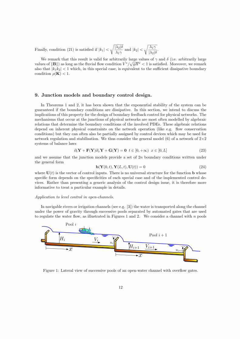
In navigable rivers or irrigation channels (see e.g. [3]) the water is transported along the channelunder the power of gravity through successive pools separated by automated gates that are usedto regulate the water flow, as illustrated in Figures 1 and 2. We consider a channel with n pools
xx
Hi
Hi+1 Vi+1
Viui
ui+1
Pool i
Pool i + 1
Figure 1: Lateral view of successive pools of an open-water channel with overflow gates.
12
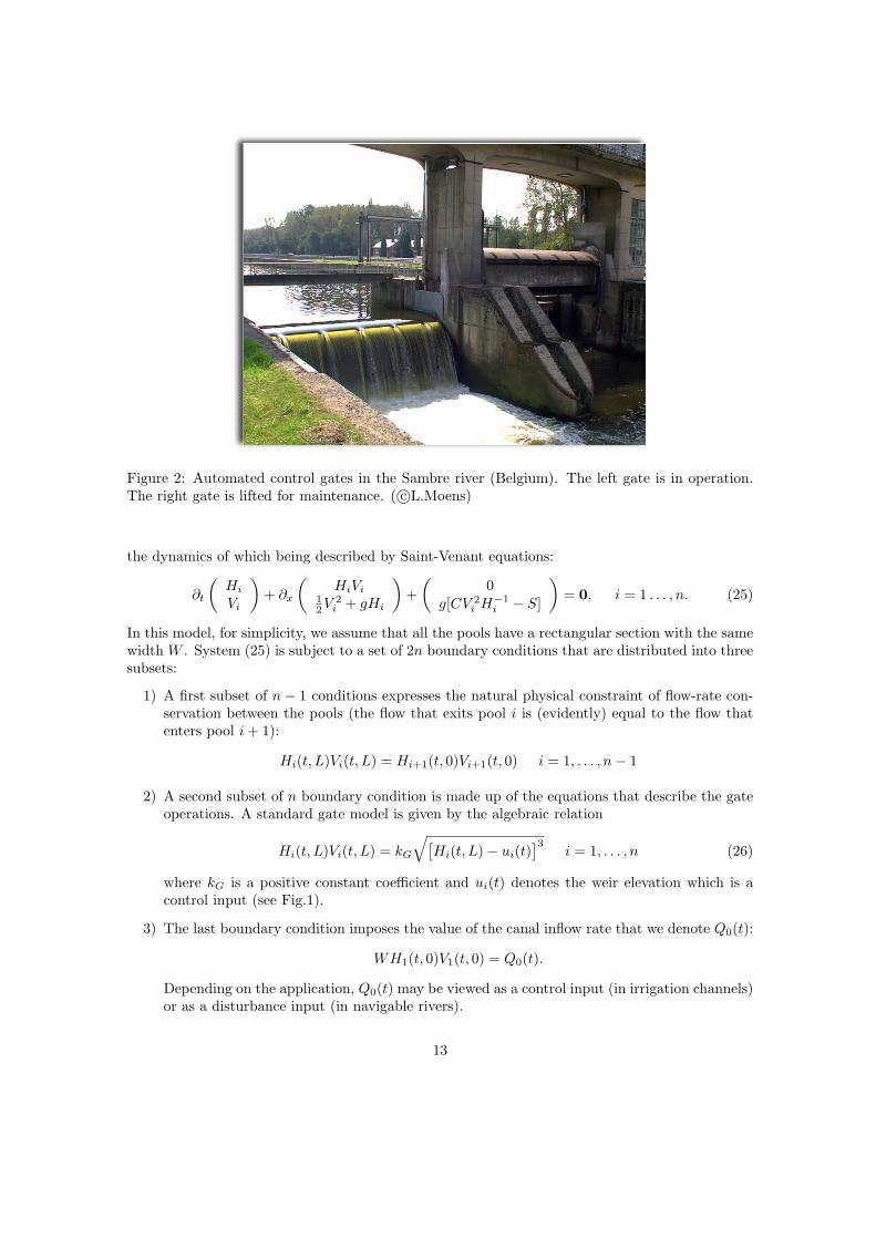
Figure 2: Automated control gates in the Sambre river (Belgium). The left gate is in operation.The right gate is lifted for maintenance. ( c©L.Moens)
the dynamics of which being described by Saint-Venant equations:
∂t
(Hi
Vi
)+ ∂x
(HiVi
12V
2i + gHi
)+(
0g[CV 2
i H−1i − S]
)= 0, i = 1 . . . , n. (25)
In this model, for simplicity, we assume that all the pools have a rectangular section with the samewidth W . System (25) is subject to a set of 2n boundary conditions that are distributed into threesubsets:
1) A first subset of n− 1 conditions expresses the natural physical constraint of flow-rate con-servation between the pools (the flow that exits pool i is (evidently) equal to the flow thatenters pool i+ 1):
Hi(t, L)Vi(t, L) = Hi+1(t, 0)Vi+1(t, 0) i = 1, . . . , n− 1
2) A second subset of n boundary condition is made up of the equations that describe the gateoperations. A standard gate model is given by the algebraic relation
Hi(t, L)Vi(t, L) = kG
√[Hi(t, L)− ui(t)
]3i = 1, . . . , n (26)
where kG is a positive constant coefficient and ui(t) denotes the weir elevation which is acontrol input (see Fig.1).
3) The last boundary condition imposes the value of the canal inflow rate that we denote Q0(t):
WH1(t, 0)V1(t, 0) = Q0(t).
Depending on the application, Q0(t) may be viewed as a control input (in irrigation channels)or as a disturbance input (in navigable rivers).
13

Boundary control design.
From Section 5, we know that the characteristic state variables of system (25) are
ξi = (Vi − V ∗i ) + (Hi −H∗i )√
g
H∗iξn+i = (Vi − V ∗i )− (Hi −H∗i )
√g
H∗ii = 1, . . . , n. (27)
Motivated by the stability analysis of the previous section, and in particular by the relation (20), wenow assume that we want the boundary conditions to satisfy the following relations in characteristiccoordinates:
ξn+i(t, L) = −kiξi(t, L) i = 1, . . . , n. (28)
with ki control tuning parameters. Then, eliminating ξi (i = 1, . . . , 2n) between (26), (27) and(28) we get the following expressions for boundary feedback control laws that realise the targetboundary conditions (28):
ui = Hi(t, L)−
[Hi(t, L)kG
(1− ki1 + ki
(Hi(t, L)−H∗i )√
g
H∗i+
√SH∗iC
)]2/3
i = 1, . . . , n. (29)
It can be seen that these control laws have the form of a state feedback. In addition, it must beemphasized that the implementation of the controls is particularly simple since only measurementsof the water levels Hi(t, L) at the gates are required. This means that the feedback implemen-tation does not require neither level measurements inside the pools nor any velocity or flow ratemeasurements.
Closed loop stability analysis.
We consider the closed loop system with a constant inflow rate Q0(t) = Q∗. We are going toexplicit sufficient conditions on the control tuning parameters ki that guarantee the dissipativityof the boundary conditions and therefore the exponential stability of the equilibrium according toTheorem 2. The first task is to express the linearisation of the boundary conditions in the form(15): (
ξ+(t, 0)ξ−(t, L))
)=(K00 K01
K10 K11
)(ξ+(t, L)ξ−(t, 0)
).
In the present application we have ξ+ , (ξ1, . . . , ξn)T and ξ− , (ξn+1, . . . , ξ2n)T . The matrix K10
is immediately given by the conditions (28):
K10 = diag−ki, i = 1, . . . , n.
Straightforward calculations show that matrices K00 and K01 and K11 are as follows:
K00 = 0 K01 = diagλn+i
λi, i = 1, . . . , n
with the characteristic velocities (see Section 5)
λi , V ∗i +√gH∗i and λn+i , V ∗i −
√gH∗i .
Finally, the matrix K11 is a n× n matrix with entries
K11[i+ 1, i] =(λi − kiλn+i)
λi+1
√H∗iH∗i+1
and 0 elsewhere.
14
Then it can be checked that, in this special case, the dissipative boundary condition ρ(K) < 1 issatisfied if the control tuning parameters ki verify the conditions:
|ki| <|λi||λn+i|
∀i ∈ 1, . . . , n.
In physical terms, this means that the control gains ki must be smaller than the ratio between thelargest and the smallest characteristic velocity in each pool.
10. Lyapunov stability analysis of nonlinear systems.
In this section we shall briefly explain how the linear Lyapunov stability analysis of Section7 can be extended to the case of the nonlinear hyperbolic system (8). Using the notations anddefinitions introduced in Section 7, the nonlinear hyperbolic system (8) in characteristic coordinatesin a neighborhood of the origin is written(
∂tξ+ + Λ+(ξ)∂xξ+
∂tξ− −Λ−(ξ)∂xξ−
)+ h(ξ) = 0 (30)
and is considered under nonlinear boundary conditions of the form(ξ+(t, 0)ξ−(t, L))
)= H
(ξ−(t, 0)ξ+(t, L))
)(31)
with a nonlinear map H : R2n → R2n.With Theorem 2 we have proved the convergence to zero of the solutions of the linear system
(14)-(15) in L2(0, L)-norm. Unfortunately the same Lyapunov function cannot be directly used toanalyse the local syability in the nonlinear case. As we have emphasized in detail in [7], in order toextend the Lyapunov stability analysis to the nonlinear case, it is needed to prove a convergencein H2(0, L)-norm. We therefore adopt the following definition of the (local) exponential stabilityof the steady-state solution ξ(t, x) ≡ 0.
Definition 2. The equilibrium solution ξ ≡ 0 of the nonlinear hyperbolic system (30)-(31) isexponentially stable (for the H2-norm) if there exist δ > 0, ν > 0 and C > 0 such that, for everyinitial condition
ξ(0, x) = ξ0(x) ∈ H2((0, 1),Rn) (32)
satisfying‖ξ0‖H2((0,1),Rn) 6 δ,
the classical solution ξ to the Cauchy problem (30)–(31)–(32) satisfies
‖ξ(t, ·)‖H2((0,1),Rn) 6 Ce−νt‖ξ0‖H2((0,1),Rn) ∀t ∈ [0,+∞). (33)
The stability property may then be generalised as follows to the nonlinear case.
Theorem 3. If ρ(H′(0)) < 1, there exists ε > 0 such that, if ‖h′(0)‖ < ε, then the equilibriumξ ≡ 0 of the nonlinear hyperbolic system (30)–(31) is exponentially stable.
15
The proof of this theorem is much more complicated than its linear counterpart and can beestablished by using the approach followed in [6]. It makes use of an augmented Lyapunov function(see (16) for comparison) of the form
V =∫ L
0
[(ξ+TP0ξ
+)e−µ1x + (ξ−TP1ξ−)eµ1x
]dx
+∫ L
0
[(∂xξ+TQ0∂xξ
+)e−µ2x + (∂xξ−TQ0∂xξ−)eµ2x
]dx
+∫ L
0
[(∂xxξ+TR0∂xxξ
+)e−µ3x + (∂xxξ−TR0∂xxξ−)eµ3x
]dx (34)
with the weighting matrices
P0 = D20(Λ+)−1 P1 = D2
1(Λ−)−1,
Q0 = D20(Λ+) Q1 = D2
1(Λ−),
R0 = D20(Λ+)3 R1 = D2
1(Λ−)3.
11. Concluding remarks and bibliographical notes.
In these lecture notes, we have been mainly concerned by the exponential stability analysis forhyperbolic systems of balance laws of the form
∂tξ + C(ξ)∂xξ + h(ξ) = 0 (35a)
(ξ+(t, 0)ξ−(t, L))
)= H
(ξ−(t, 0)ξ+(t, L))
)(35b)
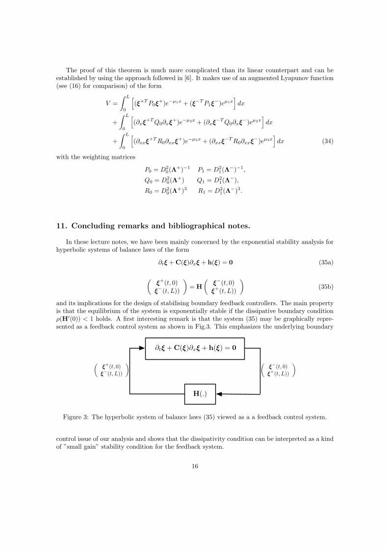
and its implications for the design of stabilising boundary feedback controllers. The main propertyis that the equilibrium of the system is exponentially stable if the dissipative boundary conditionρ(H′(0)) < 1 holds. A first interesting remark is that the system (35) may be graphically repre-sented as a feedback control system as shown in Fig.3. This emphasizes the underlying boundary
!t! + C(!)!x! + h(!) = 0
!!!(t, 0)!+(t, L))
"!!+(t, 0)!!(t, L))
"
H(.)
Figure 3: The hyperbolic system of balance laws (35) viewed as a a feedback control system.
control issue of our analysis and shows that the dissipativity condition can be interpreted as a kindof ”small gain” stability condition for the feedback system.
16
The problem of analysing the asymptotic stability of the equilibrium ξ ≡ 0 for systems ofconservation laws ∂tξ+ C(ξ)∂xξ = 0 has been considered in the literature for more than twentyyears. To our knowledge, first results were published by Slemrod [16] and by Greenberg and Li[10] for the special case of 2×2 systems. A generalization to n×n systems was given by Li and hiscollaborators (see e.g. the textbook [17]). These results were based on a systematic use of directestimates of the solutions and their derivatives along the characteristic curves. The exponentialconvergence (in C1(0, L)-norm) of the solutions towards the equilibrium was established undera sufficient dissipative boundary condition [17, Theorem 1.3, page 173] formulated as follows:ρs(|K|) < 1 (with K , H′(0) in the nonlinear case) where ρs(A) denotes the spectral radius ofA and |A| denotes the matrix whose elements are the absolute values of the elements of A. Thisapproach has been applied for the control of networks of open channels in our previous paper [8]and by Leugering and Schmitt [12].
A different approach that uses the Lyapunov function (12) has been introduced in [7] in order toanalyse the stability of systems of conservation laws under the same dissipative boundary conditionρs(|K|) < 1. The Lyapunov function is related to a similar function used in [4] for the stabilizationof the Euler equation of incompressible fluids. It is also similar to the Lyapunov function usedin [19] to analyse the stability of a general class of linear symmetric hyperbolic systems. Thecontribution of [7] was to show how this kind of Lyapunov function can be extended to the form(34) in order to prove the exponential convergence of nonlinear systems of conservation laws inH2(0, L)-norm. In addition of providing a more concise mathematical analysis, an advantage ofhaving an explicit Lyapunov function is that it is a guarantee of robustness. Finally, in the recentpapers [2] and [6], we have shown that this Lyapunov stability approach leads to a new explicitdissipative boundary condition ρ(K) < 1 (introduced in Section 7) which is weaker since it canbe shown that ρ(K) < ρs(|K|) for certain K matrices (see [6] for details). All these results wereestablished under static boundary conditions. However, for the linear case, the use of dynamicboundary conditions represented by ordinary differential equations has also been briefly addressedin [14] (including the use of PI-type feedback controllers).
In the present lecture notes, our main contribution has been to explain how this Lyapunovstability analysis can be further extended to the case of hyperbolic sytems of balance laws ∂tξ +C(ξ)∂xξ + h(ξ) = 0. In Theorem 1 we have first given a general implicit formulation of sufficientdissipative boundary conditions. Then in Theorems 2 and 3, we have shown that the explicitcondition ρ(K) < 1 also holds with a convergence in H2(0, L)-norm for sytems of balance lawsconsidered as perturbations of conservation laws. A variant of this property with convergence inC1(0, L)-norm can also be found in the reference [13]. Finally, the most interesting and originalresult is given in Section 8 where we have given an example which shows that, in particularinstances, the stability condition ρ(K) < 1 may hold even in the case of balance laws with largesource terms h(ξ) that deviate widely from the corresponding conservation laws.
References
[1] A. Aw and M. Rascle. Resurection of second-order models for traffic flow. SIAM Journal onApplied Mathematics, 60:916–938, 2000.
[2] G. Bastin, B. Haut, J-M. Coron, and B. d’Andrea-Novel. Lyapunov stability analysis ofnetworks of scalar conservation laws. Networks and Heterogeneous Media, 2(4):749 – 757,2007.
[3] M. Cantoni, E. Weyer, Y. Li, I. Mareels, and M. Ryan. Control of large-scale irrigationnetworks. Proceedings of the IEEE, 95(1):75 – 91, 2007.
17
[4] J-M. Coron. On the null asymptotic stabilization of the two-dimensional in compressibleEuler equations in a simply connected domain. SIAM Journal of Control and Optimization,37(6):1874–1896, 1999.
[5] J-M. Coron. Control and Nonlinearity, volume 136 of Mathematical Surveys and Monographs.American Mathematical Society, Providence, RI, 2007.
[6] J-M. Coron, G. Bastin, and B. d’Andrea-Novel. Dissipative boundary conditions for onedimensional nonlinear hyperbolic systems. SIAM Journal of Control and Optimization,47(3):1460 – 1498, 2008.
[7] J-M. Coron, B. d’Andrea-Novel, and G. Bastin. A strict Lyapunov function for boundarycontrol of hyperbolic systems of conservation laws. IEEE Transactions on Automatic Control,52(1):2–11, January 2007.
[8] J. de Halleux, C. Prieur, J-M. Coron, B. d’Andrea-Novel, and G. Bastin. Boundary feedbackcontrol in networks of open-channels. Automatica, 39:1365–1376, 2003.
[9] A. de Saint-Venant. Theorie du mouvement non permanent des eaux, avec application auxcrues des rivieres et a l’introduction des marees dans leur lit. Comptes rendus de l’Academiedes Sciences de Paris, Serie 1, Mathematiques, 53:147–154, 1871.
[10] J.M. Greenberg and Li Tatsien. The effect of boundary damping for the quasilinear waveequations. Journal of Differential Equations, 52:66–75, 1984.
[11] P.D. Lax. Hyperbolic systems of conservation laws and the mathematical theory of shockwaves. In Conference Board of the Mathematical Sciences Regional Conference Series inApplied Mathematics, N 11, Philadelphia, 1973. SIAM.
[12] G. Leugering and J-P.G. Schmidt. On the modelling and stabilisation of flows in networks ofopen canals. SIAM Journal of Control and Optimization, 41(1):164–180, 2002.
[13] C. Prieur, J. Winkin, and G. Bastin. Robust boundary control of systems of conservationlaws. Mathematics of Control, Signal and Systems (MCSS), in press, 2008.
[14] V. Dos Santos, G. Bastin, J-M. Coron, and B. d’Andrea-Novel. Boundary control with integralaction for hyperbolic systems of conservation laws : stability and experiments. Automatica,44(5):1310 – 1318, 2008.
[15] D. Serre. Systems of Conservation Laws. Cambridge University Press, 1999.
[16] M. Slemrod. Boundary feedback stabilization for a quasilinear wave equation. In Control The-ory for Distributed Parameter Systems, volume 54 of Lecture Notes in Control and InformationSciences, pages 221–237. Springer Verlag, 1983.
[17] Li Tatsien. Global Classical Solutions for Quasi-Linear Hyperbolic Systems. Research inApplied Mathematics. Masson and Wiley, 1994.
[18] H. Valiaho. On the definity of quadratic forms subject to linear constraints. Journal ofOptimization Theory and Applications, 38(1):143 – 145, 1982.
[19] C.Z. Xu and G. Sallet. Exponential stability and transfer functions of processes governedby symmetric hyperbolic systems. ESAIM Control Optimisation and Calculus of Variations,7:421–442, 2002.
18