using genetic algorithms for concept learningbylander/cs6243/dejong1993genetic.pdf ·...

Using Genetic Algorithms for Concept Learning

Kenneth A. De Jong, William M. Spears and Diana F. Gordon

Naval Research LaboratoryWashington, D.C. 20375

andGeorge Mason University

Fairfax, VA 22030

Abstract

In this paper, we explore the use of genetic algorithms (GAs) as a key element inthe design and implementation of robust concept learning systems. We describe andevaluate a GA-based system called GABIL that continually learns and refines conceptclassification rules from its interaction with the environment. The use of GAs ismotivated by recent studies showing the effects of various forms of bias built intodifferent concept learning systems, resulting in systems that perform well on certain con-cept classes (generally, those well matched to the biases) and poorly on others. By incor-porating a GA as the underlying adaptive search mechanism, we are able to construct aconcept learning system that has a simple, unified architecture with several importantfeatures. First, the system is surprisingly robust even with minimal bias. Second, thesystem can be easily extended to incorporate traditional forms of bias found in other con-cept learning systems. Finally, the architecture of the system encourages explicitrepresentation of such biases and, as a result, provides for an important additionalfeature: the ability to dynamically adjust system bias. The viability of this approach isillustrated by comparing the performance of GABIL with that of four other more tradi-tional concept learners (AQ14, C4.5, ID5R, and IACL) on a variety of target concepts.We conclude with some observations about the merits of this approach and about possi-ble extensions.

Key words: concept learning, genetic algorithms, bias adjustment

- 2 -

1. Introduction

An important requirement for both natural and artificial organisms is the ability toacquire concept classification rules from interactions with their environment. In thispaper, we explore the use of an adaptive search technique, namely, genetic algorithms(GAs), as the central mechanism for designing such systems. The motivation for thisapproach comes from an accumulating body of evidence that suggests that, although con-cept learners require fairly strong biases to induce classification rules efficiently, no apriori set of biases is appropriate for all concept learning tasks. We have been exploringthe design and implementation of more robust concept learning systems which are capa-ble of adaptively shifting their biases when appropriate. What we find particularly intri-guing is the natural way GA-based concept learners can provide this capability.

As proof of concept we have implemented a system called GABIL with thesefeatures and have compared its performance with four more traditional concept learningsystems (AQ14, C4.5, ID5R, and IACL) on a set of target concepts of varying complex-ity.

We present these results in the following manner. We begin by showing how con-cept learning tasks can be represented and solved by traditional GAs with minimal impli-cit bias. We illustrate this by explaining the GABIL system architecture in some detail.

We then compare the performance of this minimalist GABIL system with AQ14,C4.5, ID5R, and IACL on a set of target concepts of varying complexity. As expected,no single system is best for all of the presented concepts. However, a posteriori one canidentify the biases that were largely responsible for each system’s superiority on certainclasses of target concepts.

We then show how GABIL can be easily extended to include these biases, whichimproves system performance on various classes of concepts. However, the introductionof additional biases raises the problem of how and when to apply them to achieve thebias adjustment necessary for more robust performance.

Finally, we show how a GA-based system can be extended to dynamically adjust itsown bias in a very natural way. We support these claims with empirical studies showingthe improvement in robustness of GABIL with adaptive bias, and we conclude with a dis-cussion of the merits of this approach and directions for further research.

2. GAs and Concept Learning

Supervised concept learning involves inducing descriptions (i.e., inductivehypotheses) for the concepts to be learned from a set of positive and negative examplesof the target concepts. Examples (instances) are represented as points in an n-dimensional feature space which is defined a priori and for which all the legal values ofthe features are known. Concepts are therefore represented as subsets of points in thegiven n-dimensional space. A concept learning program is presented with both adescription of the feature space and a set of correctly classified examples of the concepts,and is expected to generate a reasonably accurate description of the (unknown) concepts.

- 3 -

The choice of the concept description language is important in several respects. Itintroduces a language bias which can make some classes of concepts easy to describewhile other class descriptions become awkward and difficult. Most of the approacheshave involved the use of classification rules, decision trees or, more recently, neural net-works. Each such choice also defines a space of all possible concept descriptions fromwhich the "correct" concept description must be selected using a given set of positive andnegative examples as constraints. In each case the size and complexity of this searchspace requires fairly strong additional heuristic pruning in the form of biases towardsconcepts which are "simpler", "more general", and so on.

The effects of adding such biases in addition to the language bias is to produce sys-tems that work well on concepts that are well-matched to these biases, but performpoorly on other classes of concepts. What is needed is a means for improving the overallrobustness and adaptability of these concept learners in order to successfully apply themto situations in which little is known a priori about the concepts to be learned. Sincegenetic algorithms (GAs) have been shown to be a powerful adaptive search techniquefor large, complex spaces in other contexts, our motivation for this work is to exploretheir usefulness in building more flexible and effective concept learners. 1

In order to apply GAs to a concept learning problem, we need to select an internalrepresentation of the space to be searched. This must be done carefully to preserve theproperties that make the GAs effective adaptive search procedures (see (DeJong, 1987)for a more detailed discussion). The traditional internal representation of GAs involvesusing fixed-length (generally binary) strings to represent points in the space to besearched. However, such representations do not appear well-suited for representing thespace of concept descriptions that are generally symbolic in nature, that have both syn-tactic and semantic constraints, and that can be of widely varying length and complexity.

There are two general approaches one might take to resolve this issue. The firstinvolves changing the fundamental GA operators (crossover and mutation) to workeffectively with complex non-string objects. Alternatively, one can attempt to construct astring representation that minimizes any changes to the GA. Each approach has certainadvantages and disadvantages. Developing new GA operators which are sensitive to thesyntax and semantics of symbolic concept descriptions is appealing and can be quiteeffective, but also introduces a new set of issues relating to the precise form such opera-tors should take and the frequency with which they should be applied. The alternativeapproach, using a string representation, puts the burden on the system designer to find amapping of complex concept descriptions into linear strings which has the property thatthe traditional GA operators that manipulate these strings preserve the syntax and seman-tics of the underlying concept descriptions. The advantage of this approach is that, if aneffective mapping can be defined, a standard "off the shelf" GA can be used with few, ifany, changes. In this paper, we illustrate the latter approach and develop a system whichuses a traditional GA with minimal changes. For examples of the other approach see(Rendell, 1985; Grefenstette, 1989; Koza, 1991; Janikow, 1991).

The decision to adopt a minimalist approach has immediate implications for thechoice of concept description languages. We need to identify a language that can be_______________

1 Excellent introductions to GAs can be found in (Holland, 1975) and (Goldberg, 1989).

- 4 -

effectively mapped into string representations and yet retains the necessary expressivepower to represent complex concept descriptions efficiently. As a consequence, we havechosen a simple, yet general rule language for describing concepts, the details of whichare presented in the following sections.

2.1. Representing the search space

A natural way to express complex concepts is as a disjunctive set of possibly over-lapping classification rules, i.e., in disjunctive normal form (DNF). The left-hand side ofeach rule (i.e., disjunct or term) consists of a conjunction of one or more tests involvingfeature values. The right-hand side of a rule indicates the concept (classification) to beassigned to the examples that are matched (covered) by the left-hand side of the rule.Collectively, a set of such rules can be thought of as representing the unknown concept ifthe rules correctly classify the elements of the feature space.

If we allow arbitrarily complex terms in the conjunctive left-hand side of such rules,we will have a very powerful description language that will be difficult to represent asstrings. However, by restricting the complexity of the elements of the conjunctions, weare able to use a string representation and standard GAs, with the only negative sideeffect that more rules may be required to express the concept. This is achieved by res-tricting each element of a conjunction to be a test of the form:

If the value of feature i of the example is in the given value set, return trueelse, return false.

For example, a rule might take the following symbolic form:

If (F1 = large) and (F2 = sphere or cube) then it is a widget.

Since the left-hand sides are conjunctive forms with internal disjunction (e.g., the dis-junction within feature F2), there is no loss of generality by requiring that there be atmost one test for each feature (on the left hand side of a rule). The result is a modifiedDNF that allows internal disjunction. (See (Michalski, 1983) for a discussion of internaldisjunction.)

With these restrictions we can now construct a fixed-length internal representationfor classification rules. Each fixed-length rule will have N feature tests, one for eachfeature. Each feature test will be represented by a fixed-length binary string, the lengthof which will depend on the type of feature (nominal, ordered, etc.). Currently, GABILonly uses features with nominal values. The system uses k bits for the k values of a nomi-nal feature. So, for example, if the set of legal values for feature F1 is {small, medium,large}, then the pattern 011 would represent the test for F1 being medium or large.

Further suppose that feature F2 has the values {sphere, cube, brick, tube} and thereare two classes, widgets and gadgets. Then, a rule for this 2 feature problem would berepresented internally as:

- 5 -

F1 F2 Class111 1000 0

This rule is equivalent to:

If (F1 = small or medium or large) and (F2 = sphere) then it is a widget.

Notice that a feature test involving all 1s matches any value of a feature and is equivalentto "dropping" that conjunctive term (i.e., the feature is irrelevant for that rule). So, in theexample above, only the values of F2 are relevant and the rule is more succinctly inter-preted as:

If (F2 = sphere) then it is a widget.

For completeness, we allow patterns of all 0s which match nothing. This means that anyrule containing such a pattern will not match any points in the feature space. While rulesof this form are of no use in the final concept description, they are quite useful as storageareas for GAs when evolving and testing sets of rules.

The right-hand side of a rule is simply the class (concept) to which the examplebelongs. This means that our rule language defines a "stimulus-response" system with nomessage passing or any other form of internal memory such as those found in (Holland,1986). In many of the traditional concept learning contexts, there is only a single con-cept to be learned. In these situations there is no need for the rules to have an explicitright-hand side, since the class is implied. Clearly, the string representation we havechosen handles such cases easily by assigning no bits for the right-hand side of each rule.

2.1.1. Sets of classification rules

Since a concept description will consist of one or more classification rules, we stillneed to specify how GAs will be used to evolve sets of rules. There are currently twobasic strategies: the Michigan approach exemplified by Holland’s classifier system (Hol-land, 1986), and the Pittsburgh approach exemplified by Smith’s LS-1 system (Smith,1983). Systems using the Michigan approach maintain a population of individual rulesthat compete with each other for space and priority in the population. In contrast, sys-tems using the Pittsburgh approach maintain a population of variable-length rule sets thatcompete with each other with respect to performance on the domain task. There is stillmuch to be learned about the relative merits of the two approaches. In this paper wereport on results obtained from using the Pittsburgh approach.2 That is, each individual inthe population is a variable-length string representing an unordered set of fixed-length_______________

2 (Greene & Smith, 1987) and (Janikow, 1991) have also used the Pittsburgh approach. See(Wilson, 1987) and (Booker, 1989) for examples of the Michigan approach.

- 6 -

rules. The number of rules in a particular individual can be unrestricted or limited by auser-defined upper bound.

To illustrate this representation more concretely, consider the following example ofa rule set with 2 rules:

F1 F2 Class F1 F2 Class100 1111 0 011 0010 0

This rule set is equivalent to:

If (F1 = small) then it is a widget.or

If ((F1 = medium or large) and (F2 = brick)) then it is a widget.

2.1.2. Rule Set Execution Semantics

In choosing a rule set representation for use with GAs, it is also important to definesimple execution semantics which encourage the development of rule subsets and theirsubsequent recombination with other subsets to form new and better rule sets. Oneimportant feature with this property is that there is no order-dependency among the rulesin a rule set. When a rule set is used to predict the class of an example, the left-handsides of all rules in a rule set are checked to see if they match (cover) a particular exam-ple. This "parallel" execution semantics means that rules perform in a location-independent manner.

It is possible that an example might be covered by more than one rule. There are anumber of existing approaches for resolving such conflicts on the basis of dynamicallycalculated rule strengths, by measuring the complexity of the left-hand sides of rules, orby various voting schemes. It is also possible that there are no rules that cover a particu-lar example. Unmatched examples could be handled by partial matching and/or coveringoperators. How best to handle these two situations in the general context of learningmultiple concepts (classes) simultaneously is a difficult issue which we have not yetresolved to our satisfaction.

However, these issues are considerably simpler when learning single concepts. Inthis case it is quite natural to view the rules in a rule set as a union of (possibly overlap-ping) covers of the concept to be learned. Hence, an example which matches one ormore rules is classified as a positive example of the concept, and an example which failsto match any rule is classified as a negative example.

In this paper, we focus on the simpler case of single-concept learning problems(which have also dominated the concept-learning literature). We have left the extensionto multi-concept problems for future work.

- 7 -

2.1.3. Crossover and mutation

Genetic operators modify individuals within a population to produce new individu-als for testing and evaluation. Historically, crossover and mutation have been the mostimportant and best understood genetic operators. Crossover takes two individuals andproduces two new individuals, by swapping portions of genetic material (e.g., bits).Mutation simply flips random bits within the population, with a small probability (e.g., 1bit per 1000). One of our goals was to achieve a concept learning representation thatcould exploit these fundamental operators. We feel we have achieved that goal with thevariable-length string representation involving fixed-length rules described in the previ-ous sections.

Our mutation operator is identical to the standard one and performs the usual bit-level mutations. We are currently using a fairly standard extension of the traditional 2-point crossover operator in order to handle variable-length rule sets. 3 With standard 2-point crossover on fixed-length strings, there are only two degrees of freedom in select-ing the crossover points since the crossover points always match up on both parents (e.g.,exchanging the segments from positions 12-25 on each parent). However, with variablelength strings there are four degrees of freedom since there is no guarantee that, havingpicked two crossover points for the first parent, the same points exist on the secondparent. Hence, a second set of crossover points must be selected for it.

As with standard crossover, there are no restrictions on where the crossover pointsmay occur (i.e., both on rule boundaries and within rules). The only requirement is thatthe corresponding crossover points on the two parents "match up semantically". That is,if one parent is being cut on a rule boundary, then the other parent must be cut on a ruleboundary. Similarly, if one parent is being cut at a point 5 bits to the right of a rule boun-dary, then the other parent must be cut in a similar spot (i.e., 5 bits to the right of somerule boundary). For example consider the following two rule sets:

F1 F2 Class F1 F2 Class

10|0 0100| 0 011 0010 0| || -------------------------| |

01|0 0001 0 110 0011| 0

We use a "|" to denote a crossover cut point. Note that the left cut point is offset 2 bitsfrom the rule boundary, while the right cut point is offset 1 bit from the rule boundary.The bits within the cut points are swapped, resulting in a rule set of 3 rules and a rule setof 1 rule:

_______________3 We are also investigating the use of a uniform crossover operator that has been recently

shown to be more effective in certain contexts than 2-point crossover.

- 8 -

F1 F2 Class F1 F2 Class F1 F2 Class

100 0001 0 110 0011 0 011 0010 0

010 0100 0

2.2. Choosing a fitness function

In addition to selecting a good representation, it is important to define a good fitnessfunction that rewards the right kinds of individuals. In keeping with our minimalist phi-losophy, we selected a fitness function involving only classification performance (ignor-ing, for example, length and complexity biases). The fitness of each individual rule set iscomputed by testing the rule set on the current set of training examples (which is typi-cally a subset of all the examples - see Section 2.6) and letting:

fitness (individual i) = (percent correct )2

This provides a bias toward correctly classifying all the examples while providing anon-linear differential reward for imperfect rule sets. This bias is equivalent to one thatencourages consistency and completeness of the rule sets with respect to the trainingexamples. A rule set is consistent when it covers no negative examples and is completewhen it covers all positive examples.

2.3. GABIL: A GA-based concept learner

We are now in a position to describe GABIL, our GA-based concept learner. At theheart of this system is a GA for searching the space of rule sets for ones that perform wellon a given set of positive and negative examples. Figure 1 provides a pseudo-codedescription of the GA used.------------------------------------------------------------------------

Insert Figure 1 about here

------------------------------------------------------------------------P(t) represents a population of rule sets. After a random initialization of the population,each rule set is evaluated with the fitness function described in section 2.2. Rule sets areprobabilistically selected for survival in proportion to their fitness (i.e., how consistentand complete they are). Crossover and mutation are then applied probabilistically to thesurviving rule sets, to produce a new population. This cycle continues until as consistentand complete a rule set as possible has been found within the time/space constraintsgiven.

Traditional concept learners differ in the ways examples are presented. Many sys-tems presume a batch mode, where all instances are presented to the system at once.Others work in an incremental mode, where one or a few of the instances are presentedto the system at a time. In designing a GA-based concept learner, the simplest approach

- 9 -

involves using batch mode, in which a fixed set of training examples is presented and theGA must search the space of variable-length strings described above for a set of ruleswith high fitness (100% implies completeness and consistency on the training set).

However, in many situations learning is a never-ending process in which new exam-ples arrive incrementally as the learner explores its environment. The examples them-selves can in general contain noise and are not carefully chosen by an outside agent.These are the kinds of problems that we are most interested in, and they imply that a con-cept learner must evolve concept descriptions incrementally from non-optimal and noisyinstances.

The simplest way to produce an incremental GA concept learner is as follows. Theconcept learner initially accepts a single example from a pool of examples and searchesfor as perfect a rule set as possible for this example within the time/space constraintsgiven. This rule set is then used to predict the classification of the next example. If theprediction is incorrect, the GA is invoked (in batch mode) to evolve a new rule set usingthe two examples. If the prediction is correct, the example is simply stored with the pre-vious example and the rule set remains unchanged. As each new additional instance isaccepted, a prediction is made, and the GA is re-run in batch mode if the prediction isincorrect. We refer to this mode of operation as batch-incremental and we refer to theGA batch-incremental concept learner as GABIL.

Although batch-incremental mode is more costly to run than batch, it provides amuch more finely-grained measure of performance that is more appropriate for situationsin which learning never stops. Rather than measure an algorithm’s performance usingonly a small training subset of the instances for learning, batch-incremental mode meas-ures the performance of this algorithm over all available instances. Therefore, everyinstance acts as both a testing instance and then a training instance.

Our ultimate goal is to achieve a pure incremental system which is capable ofresponding to even more complex situations such as when the environment itself ischanging during the learning process. In this paper, however, we report on the perfor-mance of GABIL, our batch-incremental concept learner.

3. Empirical System Comparisons

The experiments described in this section are designed to compare the predictiveperformance of GABIL and four other concept learners as a function of incrementalincreases in the size and complexity of the target concept.

3.1. The domains

The experiments involve two domains: one artificial, and one natural. Domain 1,the artificial domain, was designed to reveal trends that relate system biases to incremen-tal increases in target concept complexity. For this domain, we invented a 4 featureworld in which each feature has 4 possible distinct values (i.e., there are 256 instances inthis world).

- 10 -

Within Domain 1, we constructed a set of 12 target concepts. We varied the com-plexity of the 12 target concepts by increasing both the number of rules (disjuncts) andthe number of relevant features (conjuncts) per rule required to correctly describe theconcepts. The number of disjuncts ranged from 1 to 4, while the number of conjunctsranged from 1 to 3. Each target concept is labeled as nDmC, where n is the number ofdisjuncts and m is the number of conjuncts (see Appendix 2 for the definition of these tar-get concepts).

For each of the target concepts, the complete set of 256 instances were labeled aspositive or negative examples of the target concept. The 256 examples were randomlyshuffled and then presented sequentially in batch-incremental mode. This procedure wasrepeated 10 times (trials) for each concept and learning algorithm pair.

For Domain 2, we selected a natural domain to further test our conjectures aboutsystem biases. Domain 2 is a well-known natural database for diagnosing breast cancer(Michalski et. al., 1986). This database has descriptions of cases for 286 patients, andeach case (instance) is described in terms of 9 features. There is a small amount of noiseof unknown origin in the database manifested as cases with identical features butdifferent classifications. The target concept is considerably more complex than any of theconcepts in the nDmC world. For example, after seeing all 286 instances, the AQ14 sys-tem (also known as NEWGEM, described below) develops an inductive hypothesis hav-ing 25 disjuncts and an average of 4 conjuncts per disjunct. Since GABIL and ID5R canonly handle nominals, and the breast cancer instances have features in the form ofnumeric intervals, we converted the breast cancer (BC) database to use nominal features.This conversion necessarily loses the inherent ordering information associated withnumeric intervals. For example, the feature age is defined to have numeric intervalvalues {10-19, 20-29, ..., 90-99} in the original database, and is represented as the set{A1, A2, ..., A9} of nominals in the converted database. When using the BC database,we again randomly shuffled the instances and averaged over 10 runs.

It should be noted that all the problems in these two test domains are single-classproblems. As discussed earlier, evaluating this approach on multi-class problems is partof our future plans.

3.2. The systems

The performance of the GABIL system described in section 2.3 was evaluated onboth domains. Standard GA settings of 0.6 for 2-pt crossover and 0.001 for mutationwere used. The choice of population size was more difficult. With large, complex searchspaces, larger population sizes are preferable, but generally require more computationtime. With our unoptimized batch-incremental version of GABIL, we were able to use apopulation size of 1000 for the artificial domain. However, for the BC domain, a popula-tion size of 100 was used in order to keep the experimental computation time reason-able.4_______________

4 Our unoptimized batch-incremental version of GABIL is somewhat slower than C4.5, AQ,and IACL. It is substantially slower than ID5R. One should not conclude from this, however,that GA concept learners are inherently slower. See Janikow (1991) for details.

- 11 -

To better assess the GABIL system, four other concept learners were also evaluatedon the target concept domains. We selected four systems to represent all four combina-tions of batch and incremental modes, and two popular hypothesis forms (DNF and deci-sion trees). The chosen systems are AQ14 (Mozetic, 1985), which is based on the AQalgorithm described in (Michalski, 1983), C4.5 (Quinlan, unpublished), ID5R (Utgoff,1988), and Iba’s Algorithm Concept Learner (IACL) (Gordon, 1990), which is based onIba’s algorithm described in (Iba, 1979). AQ14 and IACL form modified DNFhypotheses. The C4.5 and ID5R systems are based on the ID algorithm described in(Quinlan, 1986), and form decision tree hypotheses. AQ14 and C4.5 are run in batch-incremental mode since they are batch systems. ID5R and IACL are incremental.

AQ14, like AQ, generates classification rules from instances using a beam search.This system maintains two sets of classification rules for each concept: one set, which wecall the positive hypothesis, is for learning the target concept and the other set, which wecall the negative hypothesis is for learning the negation of the target concept. (Note thatGABIL currently uses only a positive hypothesis.) AQ14, like GABIL, generatesclassification rules in a modified DNF that allows internal disjunction of feature values.Internal disjunction allows fewer external disjuncts in the hypotheses.

AQ14’s learning method guarantees that its inductive hypotheses will be consistentand complete with respect to all training examples. The learning method, called the StarAlgorithm, generates a hypothesis for each class C. Potential rules for this hypothesis areformed from a randomly-chosen example, called a seed, by maximally generalizing thedescription of the seed without covering any examples of the wrong class. One rule ischosen from the set of potential rules, using a user-specified set of criteria, and this rule isadded to the hypothesis for C. This procedure repeats to generate more rules for thehypothesis until all examples of class C are covered by the hypothesis.

AQ14’s criteria for hypothesis preferences (biases) influences its learning behavior.This system’s performance depends on these criteria, as well as on other parameter set-tings. The particular parameter settings that we chose for AQ14 implement a preferencefor simpler inductive hypotheses, e.g., inductive hypotheses having shorter rules.5

C4.5 uses a decision tree representation rather than a rule representation for itsinductive hypotheses. Each decision tree node is associated with an instance feature.Each node represents a test on the value of the feature. Arcs emanating from a featurenode correspond to values of that feature. Each leaf node is associated with aclassification (e.g., positive or negative if one concept is being learned). To view a deci-sion tree as a positive DNF hypothesis, one would consider this hypothesis to be the dis-junction of all paths (a conjunction of feature values) from the root to a positive leaf.The negative hypothesis is simply the disjunction of all paths from the root to a negativeleaf.

_______________5 The precise criteria used are: the positive and negative inductive hypotheses are allowed to

intersect provided the intersection covers no instances, noisy examples are considered positive,the maximum beam width is set to 20, and the minimum number of features and values arepreferred in each rule. Other settings, which have less impact on system performance, are left atdefault values.

- 12 -

An information theoretic measure biases the search through the space of decisiontrees. Trees are constructed by first selecting a root node, then the next level of nodes,and so on. Those tree nodes, or features, that minimize entropy and therefore maximizeinformation gain are selected first. The result is a preference for simpler (i.e., shorter)decision trees. C4.5 does not require completeness or consistency.

Two configurations of C4.5 are available: pruned and unpruned. Pruning is a pro-cess of further simplifying decision trees. This process, which occurs after the decisiontree has been generated, consists of testing the tree on previously seen instances andreplacing subtrees with leaves or branches whenever this replacement improves theclassification accuracy.6 Pruning is designed for both tree simplification (which increasesthe simplicity preference) and for improved prediction accuracy. Since it was not obvi-ous to us when either configuration is preferable, we used both versions in our experi-ments.

ID5R learns with the same basic algorithm as C4.5. However, this system learnsincrementally. Other than the incremental learning, ID5R’s biases are nearly identical tothose of C4.5 unpruned. One minor difference is that, unlike C4.5, ID5R does not predictthe class of a new instance when it cannot make a prediction, e.g., when the instance isnot covered by the decision tree. We have modified ID5R to make a random predictionin this case.7

The fourth system to be compared with GABIL is IACL (Gordon, 1990), a systemsimilar to AQ14. IACL is not as well-known as the other systems described above and,therefore, we describe it in slightly more detail. IACL maintains two DNF hypotheses,one for learning the target concept, and one for learning the negation of that concept.Internal disjunction is permitted, and consistency and completeness is required. UnlikeAQ14, though, IACL learns incrementally and prefers hypotheses that are more specific(i.e., less general) rather than simpler. A merging process maintains completeness. Themerging process incorporates each new instance not already covered by a hypothesis intothe hypothesis of the same class as that instance by performing a small amount of gen-eralization. This is done by forming new hypothesis rules using a most specific generali-zation (MSG) operator. From every rule in the hypotheses, IACL forms a new rule thathas feature values equal to the most specific generalization of the feature values of thenew instance and those of the original rule. Each new rule is kept only if it is consistentwith previous instances. Otherwise, the original rule is kept instead. If the instance can-not merge with any existing rule of the hypothesis, a description of it is added as a newrule.

When the features are nominals, as is the case for our experiments, the most specificgeneralization is the internal disjunction of the feature values of the rule and those of thenew instance. For example, suppose the system receives its first instance, which is posi-tive and is a small sphere. Then the initial positive hypothesis is:_______________

6 The type of pruning in C4.5 is a variant of pessimistic pruning described in (Quinlan, 1987)that prunes a tree to either a subtree or a leaf node (Quinlan, personal communication).

7 ID5R, like GABIL, is a research tool and therefore does not handle some of the realistic datacharacteristics (e.g., missing feature values) that can be handled by sophisticated systems such asC4.5.

- 13 -

if ((F1 = small) and (F2 = sphere)) then it is a widget.

If the second instance is a medium cube, and it is positive, the positive hypothesisbecomes:

if ((F1 = small or medium) and (F2 = sphere or cube)) then it is a widget

Note that this new hypothesis matches medium spheres and small cubes, though theyhave not been seen yet.

IACL’s splitting process maintains consistency. If the system incorrectly predictsthe class of a new instance, the system uses previously saved instances to relearn thehypotheses correctly. Let us continue with our example to illustrate the splitting process.Suppose the system now receives a new negative example that is a medium sphere. Thecurrent positive hypothesis matches this example, thereby violating the consistencyrequirement. After the splitting process, the positive hypothesis becomes:

if ((F1 = small) and (F2 = sphere)) then it is a widgetor

if ((F1 = medium) and (F2 = cube)) then it is a widget,

and the negative hypothesis is:

if (F1 = medium) and (F2 = sphere) then it is not a widget.

New instances can be merged with these rules to generalize the hypotheses whenevermerging preserves consistency with respect to previous instances.

3.3. Performance criteria

We feel that learning curves are an effective means for assessing performance in thecontext of incremental concept learning. In the experiments reported here, each curverepresents an average performance over 10 independent trials for learning a single targetconcept. During each trial, we keep track of a small window of recent outcomes, count-ing the correct predictions within that window. The value of the curve at each time steprepresents the percent correct achieved over the most recent window of instances. Awindow size of 10 was used for the artificial domain and one of size 50 for the BCdomain. The sizes were chosen experimentally to balance the need for capturing recentbehavior and the desire to smooth short term variations in the learning curves.

After generating learning curves for each target concept, we collapsed the informa-tion from these curves into two performance criteria. The first, called the predictionaccuracy (PA) criterion, is the average over all values on a learning curve, from the

- 14 -

beginning to the end of learning a target concept. We distilled the learning curves into asingle average value to simplify the presentation of our results. The second performancecriterion, called convergence (C), is the number of instances seen before a 95% predic-tion accuracy is maintained. If a 95% prediction accuracy can not be achieved (e.g., onthe BC database), then C is not defined. The finely-grained measure obtainable withbatch-incremental and incremental modes facilitates this performance criterion as well.

The criteria just described are local in the sense that they apply to a single targetconcept. For each local criterion there is a corresponding global criterion that considersall target concepts in a domain. The global prediction accuracy criterion is the average ofthe PA criteria values on every target concept within a domain. Likewise, the globalconvergence criterion is the average of the C criteria values on all the target concepts ofa domain. Since the global criteria are based on far more data than the local criteria, webase most of our conclusions from the experiments on the former.

3.4. Results

Table 1 shows the results of the PA and global PA (denoted ‘‘Average’’ in thetables) criteria for measuring the performance of all systems on the nDmC and BC targetconcepts, while Table 2 shows the results of applying the C and global C (denoted‘‘Average’’ in the tables) criteria to measure performance on the nDmC concepts only(since no system achieves 95% prediction accuracy on the BC database). Although thereare differences between Tables 1 and 2, the general trend is similar. From these tables wecan see that AQ14 is the best performer overall. In particular, AQ14 is the top or close tothe top performer on the nDmC concepts. This system does not, however, perform aswell as the other systems on the BC target concept (except IACL). These results are dueto the fact that AQ14, when using our chosen parameter settings, is a system that is welltuned to simpler DNF target concepts.8

------------------------------------------------------------------------

Insert Table 1 about here

------------------------------------------------------------------------------------------------------------------------------------------------


------------------------------------------------------------------------

IACL does not perform as well as the other systems on the BC target concept. Weconsider this to be a result of IACL’s sensitivity to our conversion of numeric intervals tonominals (as discussed earlier). IACL’s MSG operator is well-suited for learning when_______________

8 AQ14 does not use flexible (partial) matching of hypotheses to instances. Flexible matchingtends to improve the performance of the AQ systems (Michalski 1990). The newest version ofAQ (AQTT-15), which uses flexible matching, was unavailable at the time of this study. In thefuture, we plan to run AQTT-15 on our suite of target concepts.

- 15 -

the instance features are structured nominals (i.e., have generalization trees to structuretheir values) or numeric, but is not well-suited for learning when the features are nomi-nals. According to (Gordon, 1990), IACL performs very well on the numeric form of theBC database.9 Other experiments (not reported here) indicate that the conversion of theBC data to a nominal form does not adversely affect performance for AQ14 and C4.5.

C4.5 pruned (abbreviated C4.5P in the tables) performs well on all but the targetconcepts that have many short disjuncts. On 4D1C, which has the most short disjuncts ofany target concept in the artificial domain, all ID-based systems (C4.5 pruned andunpruned, as well as ID5R), perform poorly.10 Based on the global performance criteria,C4.5 unpruned (abbreviated C4.5U in the tables) performs the best of the ID-based sys-tems on the artificial domain, whereas C4.5 pruned performs the best on the BC domain.

GABIL appears to be a good overall performer. It does not do superbly on any par-ticular concept, but it also does not have a distinct region of the space of concepts onwhich it clearly degrades. Furthermore, GABIL is quite competitive on the difficult BCtarget concept. The statistical significance of these results is presented in Appendix 1.

It is clear from these results that none of the systems under evaluation is superior toall others on all the target concepts. The dominance of one technique on a certain class ofconcepts appears to be due in large part to the built-in forms of bias it embodies, andthese can have a negative impact on other classes of concepts.

4. A More Robust Concept Learner

The GABIL system evaluated above incorporates a "pure" GA as its search mechan-ism in the sense that there were no specific changes made to the internal representation orgenetic operators relating to the task of concept learning. As in other application tasks,this generally results in a good overall GA-based problem solver, but one that can be out-performed by task-specific approaches particularly on simpler problems (see, for exam-ple, (De Jong & Spears, 1989)). However, one of the nice properties of a GA-based sys-tem is that it is not difficult to augment GAs with task-specific features to improve perfor-mance on that task.

After obtaining the performance comparisons described in the previous section, wefelt that extending GABIL with a small set of features appropriate to concept learningwould significantly enhance its overall performance and robustness. Our approach wasas follows. Each of the traditional concept learners evaluated above appeared to containone or more biases that we considered to be largely responsible for that system’s successon a particular class of target concepts. We selected a subset of these biases to be imple-mented as additional "genetic" operators to be used by GABIL’s GA search procedure(see Figure 2). The virtue of this approach is the simple and unified way GABIL’s_______________

9 When run in batch mode on the numeric BC database, with 70% of the instances in thetraining set and 30% in the test set, 72% of the predictions made on the test set were correctpredictions (see Gordon, 1990).

10 An explanation of the difficulty of systems based on ID3 on target concepts of this type is in(De Jong & Spears, 1991).

- 16 -

underlying search process can be extended to include various traditional forms of con-cept learning bias.------------------------------------------------------------------------


------------------------------------------------------------------------

Since AQ14 seemed to be the best overall performer, we selected it as our initialsource of additional operators for GABIL. As we have described above, the AQ14 sys-tem used in our experiments has preferences for simpler and more general rules. Afterstudying the results of our initial evaluation, we hypothesized that this is one of thebiases largely responsible for AQ14’s superior performance on the nDmC concepts. Thisanalysis led to the addition of two new GABIL operators which add biases for simplerand more general descriptions.

4.1. The adding alternative operator

One of the mechanisms AQ uses to increase the generality of its inductivehypotheses is the "adding alternative" generalization operator of (Michalski, 1983). Thisoperator generalizes by adding a disjunct (i.e., alternative) to the current classificationrule. The most useful form of this operator, according to (Michalski, 1983), is the addi-tion of an internal disjunct. For example, if the disjunct is

(F1 = small) and (F2 = sphere)

then the adding alternative operator might create the new disjunct

(F1 = small) and (F2 = sphere or cube).

This operator, which we call AA (the adding alternative operator), is easily implementedin GABIL by including an additional mutation that, unlike the normal mutation operator,has an asymmetric mutation rate. In particular, in the studies reported here, this operatorincorporates a 75% probability of mutating a bit to a 1, but a 25% probability of mutatingit to a 0. Therefore, the AA operator in GABIL has a strong preference for adding inter-nal disjuncts. To illustrate, the adding alternative operator might change the disjunct

F1 F2100 100

to

F1 F2100 110

- 17 -

Note that feature F2 has been generalized in this disjunct.

As with the other genetic operators, the adding alternative operator is applied pro-babilistically to a subset of the population each generation. In the studies reported here itwas applied at a rate of 0.01 (1%). 11 For clarity in reporting the experimental results, wecall the version of GABIL with the adding alternative operator ‘‘GABIL+A’’.

4.2. The dropping condition operator

A second, and complementary, generalization mechanism leading to simplerhypotheses involves removing what appear to be nearly irrelevant conditions from a dis-junct. This operator, which we call DC (the dropping condition operator), is based onthe generalization operator of the same name described in (Michalski, 1983). For exam-ple, if the disjunct is

(F1 = small or medium) and (F2 = sphere)

then the DC operator might create the new disjunct

(F2 = sphere).

The DC operator is easily added to GABIL in the following manner. When thisoperator is applied to a particular member of the population (i.e., a particular rule set),each disjunct is deterministically checked for possible condition dropping. The decisionto drop a condition is based on a criterion from (Gordon, 1990) and involves examiningthe bits of each feature in each disjunct. If more than half of the bits of a feature in a dis-junct are 1s, then the remaining 0 bits are changed to 1s. By changing the feature to haveall 1 values, this operator forces the feature to become irrelevant within that disjunct andthereby simulates the effect of a shortened disjunct. To illustrate, suppose this operator isapplied to the following disjunct:

F1 F2110 100

Then the dropping condition operator will result in a new disjunct as follows:

F1 F2111 100

Note that feature F1 is now irrelevant within this disjunct._______________

11 Note that this is in addition to the standard mutation operator, which continues to fire with aprobability of .001.

- 18 -

As with the other genetic operators, this new operator is applied probabilistically toa subset of the population each generation. In the experiments reported here, a rate of0.60 (60%) was used. We make no claim that the rates used for either of these newoperators are in any sense optimal. In these studies we selected a rate which seemed rea-sonable on the basis of a few informal experiments. Our preference (see section 5) is thatsuch things be self-adaptive.

We call GABIL with the DC operator ‘‘GABIL+D’’. When both task-specificoperators are added to GABIL, the resulting system is called ‘‘GABIL+AD’’ (see Figure3). Note that there is an interesting complementary relationship between these twooperators in that adding alternatives can set the stage for dropping a condition altogether.------------------------------------------------------------------------


------------------------------------------------------------------------

These augmented forms of GABIL do not change in any way the overall structureof the GA-based system described earlier (compare Figures 1 & 3). The only differenceis that the set of "genetic" operators has been expanded. The result is that, after the tradi-tional crossover and mutation operators have been used in the normal manner to producenew offspring (rule sets) from parents, the two new operators are (probabilistically)applied to each offspring, producing additional task-specific changes.

4.3. Results

To study the effects of adding these bias operators to GABIL, GABIL+A,GABIL+D, and GABIL+AD have been run on the same concept domains used earlier.Table 3 shows the results of system performance measured using the PA and global PAcriteria. Table 4 shows the results of system performance measured using the C and glo-bal C criteria. GABIL is abbreviated ‘‘G’’ in the tables.------------------------------------------------------------------------


------------------------------------------------------------------------------------------------------------------------------------------------


------------------------------------------------------------------------

According to the global criteria in Tables 3 and 4, GABIL+A does not perform aswell as GABIL+D or GABIL+AD. On the BC target concept, the combination of bothoperators (GABIL+AD) is the best. It is interesting to note, however, that on the nDmCdomain, GABIL+AD does not perform as well as GABIL+D.

These results indicate that one can improve GABIL’s performance on certainclasses of concepts by the addition of an appropriate set of bias operators. On the other

- 19 -

hand, it is not possible in general to know beforehand which set of biases is best. Theseresults also point out the danger of indiscriminately including multiple biases as a stra-tegy for overcoming this lack of a priori knowledge since multiple simultaneous biasescan in fact interfere with one another, leading to a degradation in performance. Theseresults, which confirm similar bias problems exhibited in other contexts, motivated us tofocus on a more sophisticated way of improving GABIL’s overall robustness, namely, byhaving it dynamically adjust its own task-specific biases.

5. An Adaptive GA Concept Learner

Although genetic algorithms themselves represent a robust adaptive search mechan-ism, most GA implementations involve static settings for such things as the populationsize, the kind of representation and operators used, and the operator probabilities. Therehave been a number of attempts to make these aspects of GAs more adaptive. We pro-vide a brief overview of this work in the next section.

5.1. Adaptive GAs

There have been two approaches to building more adaptive GAs, which we refer toas the within-problem approach and the across-problem approach. The within-problemapproach adapts a GA dynamically, as it solves one problem. In contrast, the across-problem approach adapts GAs over the course of many problems. One good example ofthe across-problem approach is provided by (Grefenstette, 1986). In this paper, aseparate meta-GA is used to adapt a GA as it solves a suite of problems. The advantageof such an approach is that the resulting system performs robustly on a suite of problems.Unfortunately, the approach is also time consuming, since each problem must be solved alarge number of times. Furthermore, the adaptation is coarse, in the sense that the systemis not necessarily optimal on any given problem. Within-problem adaptation provides afiner-grained approach, since the GA is adapted while one problem is solved. Further-more, since the problem is solved only once, the approach can require much less time.We concentrate on the within-problem approach, since we wish to adapt the GA as itsolves each concept learning problem.

Within-problem approaches can be further divided into two categories, coupled anduncoupled, based on the observation that an adaptive GA is in effect searching twospaces: the original problem space, and the space of adaptations to the underlying GAitself. The relationship of these two search processes is an important design considera-tion for adaptive GAs.

In a coupled approach, both searches are handled simultanously by a single GAsearch procedure. This is accomplished by using the underlying population to storeinformation relevant to the adaptive mechanism as well as the standard informationregarding the original problem space being searched. This approach is elegant andstraightforward, since no new adaptive mechanism is required (see (Schaffer, 1987) forexamples of this approach). Unfortunately, this coupling also means that the additionalsearch can be hindered by the same issues that hinder the search of the problem space.For example, one possible concern is that this mechanism may only work well with large

- 20 -

population sizes. As with any other statistical sampling algorithm, small populations(samples) may be misleading and lead to wrong conclusions. This issue will be raisedagain later in this paper.

An uncoupled approach does not rely upon the GA for the adaptive mechanism.Rather, the behavior of the underlying GA is adjusted by a separate control mechanism(see (Davis, 1989) and (Janikow, 1991) for examples). While this may alleviate theproblems associated with coupling, such mechanisms appear to be difficult to construct,and involve complicated bookkeeping. Although we may explore this route in futurework, we concentrate on the conceptually simpler coupled approach in this paper. Wenext consider how to implement a coupled within-problem approach within GABIL.

5.2. Adaptive GABIL

Recall that the task-specific operators added to GABIL (DC and AA) were added ina static way. That is, they were either present or not present for an entire experiment. Ifthey were present, they were applied via fixed probabilities to all new individuals. Thesimplest coupled way to make the selection and application of these operators moreadaptive is to have each individual specify which operators can be applied to it. Theintuition here is that those individuals which enable the "correct" operators will be morefit from a survival point of view. The result should be a system capable of performingthe search for the best set of operators (biases) and the search for the best hypotheses inparallel (see (Baeck et. al., 1991) for related work).

Such an approach is easily implemented by adding to each individual additionalcontrol bits (one for each adaptive operator). Each bit determines whether thecorresponding operator can be used on that individual. If the control bit is 0, the associ-ated operator is not permissible, and can not be fired (thus ignoring the operator probabil-ity). If the control bit is 1, the associated operator is permissible, and fires according tothe relevant operator probability. These control bits act as added Boolean preconditionsfor the operators. The values of the control bits are evolved in the normal way throughselection, crossover, and mutation.12

As an initial test of this approach, GABIL was modified to include two extra controlbits, one for each of the task-specific operators introduced earlier. For example, considerthe following rule set:

F1 F2 Class F1 F2 Class D A010 001 0 110 011 0 1 0

The two added control bits are indicated with the letters "D" and "A" (for dropping condi-tion and adding alternative, respectively). For this rule set the dropping condition opera-tor is permissible, while the adding alternative operator is not. So, for example, the DCoperator would change the rule set to:_______________

12 The dropping condition and adding alternative operators do not alter these control bits.

- 21 -

F1 F2 Class F1 F2 Class D A010 001 0 111 111 0 1 0

We call this modified system ‘‘adaptive GABIL’’, and have begun to explore itspotential for effective dynamic bias adjustment. To get an immediate and direct com-parison with the earlier results, adaptive GABIL was run on the nDmC and BC targetconcepts. The results are presented in Tables 5 and 6.------------------------------------------------------------------------


------------------------------------------------------------------------------------------------------------------------------------------------


------------------------------------------------------------------------

The results of the global criteria, shown at the bottom of Tables 5 and 6, highlight acouple of important points. First, on the nDmC domain, the adaptive GABIL outperformsthe original GABIL, GABIL+A, and GABIL+AD. Furthermore, the adaptive GABILperforms almost as well as GABIL+D from a prediction accuracy criterion, and betterfrom a convergence criterion. Adaptive GABIL outperforms GABIL+AD, particularlyfrom the standpoint of the global C criterion. This shows the danger of indiscriminatelyincluding multiple fixed biases, which can interfere with each other, producing lowerperformance. These results demonstrate the virtues of adaptive GABIL in selecting theappropriate biases.

On the BC target concept, adaptive GABIL performs better than GABIL andGABIL+A, but is worse than GABIL+D and GABIL+AD. This suggests that adaptiveGABIL’s advantage is diminished when smaller population sizes (e.g., population sizesof 100) are involved. To address this issue, future versions of GABIL will have to adaptthe population size, as well as operator selection.

In comparison to the other systems, the new adaptive GABIL is much better thanC4.5 on the nDmC domain, and close on the BC target concept. Also, adaptive GABIL iscompetitive with AQ14 on the nDmC domain, and is much better on the BC target con-cept. We have tested the statistical significance of these results (see Appendix 1), andfound that when adaptive GABIL outperforms other systems, the results are generallysignificant (at a 90% level). Furthermore, when other systems outperform adaptiveGABIL, the results are generally not significant (i.e., significance is 80% or lower). Theonly two notable exceptions are on the BC database. Both C4.5 and GABIL+AD outper-form adaptive GABIL at a 95% level of significance. We believe that the latter excep-tion is due to the small population size (100). The former exception will be addressedwhen we incorporate C4.5’s information theoretic biases into GABIL. This bias can bequite easily implemented as a "genetic" operator by making features with higher entropyvalues more likely to have 1s (since higher entropy values imply less relevance).

- 22 -

An interesting question at this point is whether the improved performance of adap-tive GABIL is the result of any significant bias adjustment during a run. This is easilymonitored and displayed. Figures 4 and 5 illustrate the frequency with which the drop-ping condition (DC) and adding alternative (AA) operators are used by adaptive GABILfor two target concepts: 3D3C and 4D1C. Since the control bits for each operator arerandomly initialized, roughly half of the initial population contain positive control bitsresulting in both operators starting out at a rate of approximately 0.5. As the searchprogresses towards a consistent and complete hypothesis, however, these frequencies areadaptively modified. For both target concepts, the DC operator is found to be the mostuseful, and consequently is fired with a higher frequency. This is consistent with Table 5,which indicates that GABIL+D outperforms GABIL+A. Furthermore, note thedifference in predictive accuracy between GABIL and GABIL+D on the two target con-cepts. The difference is greater for the 4D1C target concept, indicating the greaterimportance of the DC operator. This is reflected in Figures 4 and 5, in which the DCoperator evolves to a higher firing frequency on the 4D1C concept, in comparison withthe 3D3C concept. Similar comparisons can be made with the AA operator.------------------------------------------------------------------------

Insert Figures 4 and 5 about here

------------------------------------------------------------------------

Considering that GABIL is now clearly performing the additional task of selectingappropriate biases, these results are very encouraging. We are in the process of extendingand refining GABIL as a result of the experiments described here. We are also extendingour experimental analysis to include other systems which attempt to dynamically adjusttheir bias.

6. Related Work on Bias Adjustment

Adaptive bias, in our context, is similar to dynamic preference (bias) adjustment forconcept learning (see (Gordon, 1990) for related literature). The vast majority of conceptlearning systems that adjust their bias focus on changing their representational bias. Thefew notable exceptions that adjust the algorithmic bias include the Competitive RelationLearner and Induce and Select Optimizer combination (CRL/ISO) (Tcheng et. al., 1989),Climbing in the Bias Space (ClimBS) (Provost, 1991), PEAK (Holder, 1990), the Vari-able Bias Management System (VBMS) (Rendell et. al., 1987), and the Genetic-basedInductive Learner (GIL) (Janikow, 1991).

We can classify these systems according to the type of bias that they select. Adap-tive GABIL shifts its bias by dynamically selecting generalization operators. The set ofbiases considered by CRL/ISO includes the strategy for predicting the class of newinstances and the method and criteria for hypothesis selection. The set of biases con-sidered by ClimBS includes the beam width of the heuristic search, the percentage of thepositive examples a satisfactory rule must cover, the maximum percentage of the nega-tive examples a satisfactory rule may cover, and the rule complexity. PEAK’s

- 23 -

changeable algorithmic biases are learning algorithms. They are rote learning, empiricallearning (with a decision tree), and explanation-based generalization (EBG). GIL is mostsimilar to GABIL, since it also selects between generalization operators. However, itdoes not use a GA for that selection and only uses a GA for the concept learning task.

We can also classify these systems according to whether or not their searchesthrough the space of hypotheses and the space of biases are coupled. GABIL is uniquealong this dimension because it is the only system that couples these searches. Theadvantages and disadvantages of a coupled approach were presented in Section 5. Wesummarize these comparisons in Table 7.------------------------------------------------------------------------


------------------------------------------------------------------------

The VBMS system is different from the others mentioned above. The primary taskof this system is to identify the concept learner (which implements a particular set ofalgorithmic biases) that is best suited for each problem along a set of problem charac-teristic dimensions. Problem characteristic dimensions that this system considers are thenumber of training instances and the number of features per instance. Three conceptlearners are tested for their suitability along these problem characteristic dimensions.VBMS would be an ideal companion to any of the above-mentioned systems. This sys-tem could map out the suitability of biases to problems, and then this knowledge could bepassed on to the other systems to use in an initialization procedure for constraining theirbias space search.

7. Discussion and Future Work

We have presented a method for using genetic algorithms as a key element indesigning robust concept learning systems and used this approach to implement a systemthat compares favorably with other concept learning systems on a variety of target con-cepts. We have shown that, in addition to providing a minimally biased yet powerfulsearch strategy, the GABIL architecture allows for adding task-specific biases in a verynatural way in the form of additional "genetic" operators, resulting in performanceimprovements on certain classes of concepts. However, the experiments in this paperhighlight that no one fixed set of biases is appropriate for all target concepts. In responseto these observations, we have shown that this approach can be further extended to pro-duce a concept learner that is capable of dynamically adjusting its own bias in responseto the characteristics of the particular problem at hand. Our results indicate that this is apromising approach for building concept learners which do not require a "human in theloop" to adapt and adjust the system to the requirements of a particular class of concepts.

The current version of GABIL adaptively selects between two forms of bias takenfrom a single system (AQ14). In the future, we plan to extend this set of biases to includeadditional biases from AQ14 and other systems. For example, we would like to imple-ment in GABIL an information theoretic bias, which we believe is primarily responsiblefor C4.5’s successes.

- 24 -

The results presented here have all involved single-class learning problems. Animportant next step is to extend this method to multi-class problems. We have also beenfocusing on adjusting the lower level biases of learning systems. We believe that thesesame techniques can also be applied to the selection of higher level mechanisms such asinduction and analogy. Our final goal is to produce a robust learner that dynamicallyadapts to changing concepts and noisy learning conditions, both of which are frequentlyencountered in realistic environments.

Acknowledgements

We would like to thank the Machine Learning Group at NRL for their useful com-ments about GABIL, J. R. Quinlan for C4.5, and Zianping Zhang and Ryszard Michalskifor AQ14.

References

Baeck, T., Hoffmeister, F., & Schwefel, H. (1991). A survey of evolution strategies.Proceedings of the Fourth International Conference on Genetic Algorithms (pp. 2 -9). La Jolla, CA: Morgan Kaufmann. 1991.

Booker, L. (1989). Triggered rule discovery in classifier systems. Proceedings of theThird International Conference on Genetic Algorithms (pp. 265 - 274). Fairfax, VA:Morgan Kaufmann.

Braudaway, W. & Tong, C. (1989). Automated synthesis of constrained generators.Proceedings of the Eleventh International Joint Conference on Artificial Intelligence(pp. 583 - 589). Detroit, MI: Morgan Kaufmann.

Davis, L. (1989). Adapting operator probabilities in genetic algorithms. Proceedings ofthe Third International Conference on Genetic Algorithms (pp. 61 - 69). Fairfax,VA: Morgan Kaufmann.

De Jong, K. (1987). Using genetic algorithms to search program spaces. Proceedings ofthe Second International Conference on Genetic Algorithms (pp. 210 - 216). Cam-bridge, MA: Lawrence Erlbaum.

De Jong, K. & Spears, W. (1989). Using genetic algorithms to solve NP-complete prob-lems. Proceedings of the Third International Conference on Genetic Algorithms (pp.124 - 132). Fairfax, VA: Morgan Kaufmann.

De Jong, K. & Spears, W. (1991). Learning concept classification rules using geneticalgorithms. Proceedings of the Twelfth International Joint Conference on ArtificialIntelligence (pp. 651 - 656). Sydney, Australia: Morgan Kaufmann.

Goldberg, D. (1989). Genetic algorithms in search, optimization, and machine learning.

- 25 -

New York: Addison-Wesley.

Gordon, D. (1990). Active bias adjustment for incremental, supervised concept learning.Doctoral dissertation, Computer Science Department, University of Maryland, Col-lege Park, MD.

Greene, D. & Smith, S. (1987). A genetic system for learning models of consumerchoice. Proceedings of the Second International Conference on Genetic Algorithms(pp. 217 - 223). Cambridge, MA: Lawrence Erlbaum.

Grefenstette, John J. (1986). Optimization of control parameters for genetic algorithms.IEEE Transactions on Systems, Man, and Cybernetics, Vol. SMC-16, No. 1.

Grefenstette, John J. (1989). A system for learning control strategies with genetic algo-rithms. Proceedings of the Third International Conference on Genetic Algorithms(pp. 183 - 190). Fairfax, Virginia: Morgan Kaufmann.

Holder, L. (1990). The general utility problem in machine learning. Proceedings of theSeventh International Conference on Machine Learning (pp. 402 - 410). Austin,Texas: Morgan Kaufmann.

Holland, J. (1975). Adaptation in natural and artificial systems. Ann Arbor, MI: TheUniversity of Michigan Press.

Holland, J. (1986). Escaping brittleness: The possibilities of general-purpose learningalgorithms applied to parallel rule-based systems. In R. Michalski, J. Carbonell, T.Mitchell (Eds.), Machine Learning: An Artificial Intelligence Approach. Los Altos:Morgan Kaufmann.

Iba, G. (1979). Learning disjunctive concepts from examples. Massachusetts Institute ofTechnology A.I. Memo 548, Cambridge, MA.

Janikow, C. (1991). Inductive learning of decision rules from attribute-based examples:A knowledge-intensive genetic algorithm approach. TR91-030, The University ofNorth Carolina at Chapel Hill, Dept. of Computer Science, Chapel Hill, NC.

Koza, J. R. (1991). Concept formation and decision tree induction using the genetic pro-gramming paradigm. In H. P. Schwefel and R. Maenner (Eds.), Parallel ProblemSolving from Nature. Berlin: Springer-Verlag.

Michalski, R. (1983). A theory and methodology of inductive learning. In R. Michalski,J. Carbonell, T. Mitchell (Eds.), Machine Learning: An Artificial IntelligenceApproach. Palo Alto: Tioga.

Michalski, R. (1986). Learning flexible concepts: Fundamental ideas and a methodbased on two-tiered representation. In Y. Kodratoff, R. Michalski (Eds.), MachineLearning: An Artificial Intelligence Approach. San Mateo: Morgan Kaufmann.

- 26 -

Michalski, R., Mozetic, I., Hong, J., & Lavrac, N. (1986). The AQ15 inductive learningsystem: An overview and experiments. University of Illinois Technical ReportNumber UIUCDCS-R-86-1260, Urbana-Champaign, ILL.

Mozetic, I. (1985). NEWGEM: Program for learning from examples, program documen-tation and user’s guide. University of Illinois Report Number UIUCDCS-F-85-949,Urbana-Champaign, ILL.

Provost, F. (1991). Navigation of an extended bias space for inductive learning, Ph.D.thesis proposal, University of Pittsburgh, Pittsburgh, PA.

Quinlan, J. (1986). Induction of decision trees. Machine Learning, 1(1), 81-106.

Quinlan, J. (1989). Documentation and user’s guide for C4.5. (unpublished).

Rendell, L. (1985). Genetic plans and the probabilistic learning system: Synthesis andresults. Proceedings of the First International Conference on Genetic Algorithms(pp. 60 - 73). Pittsburgh, PA: Lawrence Erlbaum.

Rendell, L., Seshu, R., & Tcheng, D. (1987). More robust concept learning usingdynamically-variable bias. Proceedings of the Fourth International Workshop onMachine Learning (pp. 66 - 78). Irvine, CA: Morgan Kaufmann.

Schaffer, J. David & Morishima, A. (1987). An adaptive crossover distribution mechan-ism for genetic algorithms. Proceedings of the Second International Conference onGenetic Algorithms (pp. 36 - 40). Cambridge, MA: Lawrence Erlbaum.

Smith, S. (1983). Flexible learning of problem solving heuristics through adaptive search.Proceedings of the Eighth International Joint Conference on Artificial Intelligence(pp. 422 - 425). Karlsruche, Germany: William Kaufmann.

Tcheng, D., Lambert, B., Lu, S., & Rendell, R. (1989). Building robust learning systemsby combining induction and optimization. Proceedings of the Eleventh InternationalJoint Conference on Artificial Intelligence (pp. 806 - 812). Detroit, MI: MorganKaufmann.

Wilson, S. (1987). Quasi-Darwinian learning in a classifier system. Proceedings of theFourth International Workshop on Machine Learning (pp. 59 - 65). Irvine, CA:Morgan Kaufmann.

Utgoff, P. (1988). ID5R: An incremental ID3. Proceedings of the Fifth InternationalConference on Machine Learning (pp. 107 - 120). Ann Arbor, Michigan: MorganKaufmann.

- 27 -

Appendix 1: Statistical Significance

The following three tables give statistical significance results. Table 8 comparesadaptive GABIL with all other systems on the nDmC domain (using predictive accu-racy). Table 9 makes the same comparison with the convergence criterion. Table 10 com-pares adaptive GABIL with all other systems on the BC target concept. The column Sigdenotes the level of significance of each comparison. The Wins column is "Yes" if adap-tive GABIL outperformed the other system; otherwise it is "No".

In comparison with all other systems, adaptive GABIL has 19 wins, 7 losses, and 1tie. At the 90% level of significance, 11 wins and 2 losses are significant. In comparisonwith the non-GA systems, adaptive GABIL has 10 wins, 4 losses, and 1 tie. Again, at the90% level of significance, 6 wins and 1 loss are significant.------------------------------------------------------------------------


------------------------------------------------------------------------------------------------------------------------------------------------


------------------------------------------------------------------------------------------------------------------------------------------------


------------------------------------------------------------------------

- 28 -

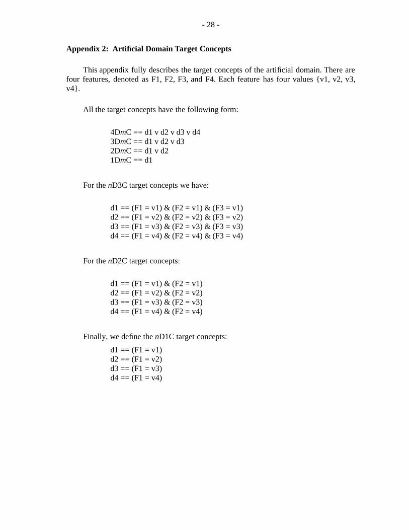
Appendix 2: Artificial Domain Target Concepts

This appendix fully describes the target concepts of the artificial domain. There arefour features, denoted as F1, F2, F3, and F4. Each feature has four values {v1, v2, v3,v4}.

All the target concepts have the following form:

4DmC == d1 v d2 v d3 v d43DmC == d1 v d2 v d32DmC == d1 v d21DmC == d1

For the nD3C target concepts we have:

d1 == (F1 = v1) & (F2 = v1) & (F3 = v1)d2 == (F1 = v2) & (F2 = v2) & (F3 = v2)d3 == (F1 = v3) & (F2 = v3) & (F3 = v3)d4 == (F1 = v4) & (F2 = v4) & (F3 = v4)

For the nD2C target concepts:

d1 == (F1 = v1) & (F2 = v1)d2 == (F1 = v2) & (F2 = v2)d3 == (F1 = v3) & (F2 = v3)d4 == (F1 = v4) & (F2 = v4)

Finally, we define the nD1C target concepts:

d1 == (F1 = v1)d2 == (F1 = v2)d3 == (F1 = v3)d4 == (F1 = v4)

- 29 -

procedure GA;begint = 0;initialize population P(t);fitness P(t);until (done)

t = t + 1;select P(t) from P(t-1);crossover P(t);mutate P(t);fitness P(t);

end.

Figure 1. The GA in GABIL.

- 30 -


t = t + 1;select P(t) from P(t-1);crossover P(t);mutate P(t);new_op1 P(t); /* additional operators */new_op2 P(t);...fitness P(t);

end.

Figure 2. Extending GABIL’s GA Operators.

- 31 -


t = t + 1;select P(t) from P(t-1);crossover P(t);mutate P(t);add_altern P(t); /* +A */drop_cond P(t); /* +D */fitness P(t);

end.

Figure 3. Extended GABIL.

- 32 -

Generations

Figure 4: 3D3C.

Rate

0

0.5

1

0 200 400

DC

AA

Generations

Figure 5: 4D1C.

Rate

0

0.5

1

0 10 20 30

DC

AA

- 33 -

Table 1. Prediction accuracy.

__________________________________________________________Prediction Accuracy____________________________________________________________________________________________________________________

TC AQ14 C4.5P C4.5U ID5R IACL GABIL__________________________________________________________1D1C 99.8 98.5 99.8 99.8 98.1 95.2__________________________________________________________1D2C 98.4 96.1 99.1 99.0 96.7 95.8__________________________________________________________1D3C 97.4 98.5 99.0 99.1 90.4 95.7__________________________________________________________2D1C 98.6 93.4 98.2 97.9 95.6 92.0__________________________________________________________2D2C 96.8 94.3 98.4 98.2 94.5 92.7__________________________________________________________2D3C 96.7 96.9 97.6 97.9 95.3 94.6__________________________________________________________3D1C 98.0 78.8 92.4 91.2 93.2 90.4__________________________________________________________3D2C 95.5 92.2 97.4 96.7 92.1 90.3__________________________________________________________3D3C 95.3 95.4 96.6 95.6 94.9 92.8__________________________________________________________4D1C 95.8 66.4 77.0 70.2 92.3 89.6__________________________________________________________4D2C 93.8 90.5 95.2 81.3 89.5 87.4__________________________________________________________4D3C 93.5 93.8 95.1 90.3 94.2 88.9____________________________________________________________________________________________________________________

Average 96.6 91.2 95.5 93.1 93.9 92.1____________________________________________________________________________________________________________________BC 60.5 72.4 65.9 63.4 60.1 68.7__________________________________________________________

��

��

��

- 34 -

Table 2. Convergence to 95%.

_____________________________________________________Convergence__________________________________________________________________________________________________________

TC AQ14 C4.5P C4.5U ID5R IACL GABIL_____________________________________________________1D1C 13 37 14 12 33 87_____________________________________________________1D2C 28 155 24 26 91 100_____________________________________________________1D3C 57 0 0 0 96 96_____________________________________________________2D1C 28 100 37 44 61 109_____________________________________________________2D2C 43 126 32 40 139 148_____________________________________________________2D3C 86 181 86 75 134 249_____________________________________________________3D1C 34 253 149 137 203 103_____________________________________________________3D2C 78 122 45 52 141 125_____________________________________________________3D3C 195 253 135 123 125 225_____________________________________________________4D1C 82 253 253 255 222 131_____________________________________________________4D2C 78 113 55 255 188 142_____________________________________________________4D3C 154 253 134 224 138 229__________________________________________________________________________________________________________

Average 73 154 80 104 131 145_____________________________________________________��

��

��

- 35 -


_________________________________________Prediction Accuracy__________________________________________________________________________________

TC GABIL G+A G+D G+AD_________________________________________1D1C 95.2 96.1 97.7 97.7_________________________________________1D2C 95.8 96.2 97.4 97.3_________________________________________1D3C 95.7 95.7 96.7 96.7_________________________________________2D1C 92.0 93.1 97.4 97.0_________________________________________2D2C 92.7 95.0 96.3 96.9_________________________________________2D3C 94.6 94.5 95.8 95.0_________________________________________3D1C 90.4 91.9 96.0 96.6_________________________________________3D2C 90.3 91.6 94.5 94.6_________________________________________3D3C 92.8 92.7 94.2 92.9_________________________________________4D1C 89.6 90.9 95.1 95.2_________________________________________4D2C 87.4 89.7 93.0 92.7_________________________________________4D3C 88.9 89.2 92.3 90.0__________________________________________________________________________________

Average 92.1 93.1 95.5 95.2__________________________________________________________________________________BC 68.7 69.1 71.5 72.0_________________________________________

��

��

��

- 36 -


______________________________________Convergence____________________________________________________________________________

TC GABIL G+A G+D G+AD______________________________________1D1C 87 58 28 32______________________________________1D2C 100 85 59 68______________________________________1D3C 96 97 94 97______________________________________2D1C 109 90 42 42______________________________________2D2C 148 93 82 55______________________________________2D3C 249 250 136 250______________________________________3D1C 103 104 54 39______________________________________3D2C 125 127 76 62______________________________________3D3C 225 240 161 240______________________________________4D1C 131 120 67 62______________________________________4D2C 142 133 75 75______________________________________4D3C 229 253 166 248____________________________________________________________________________

Average 145 138 87 106______________________________________��

��

��

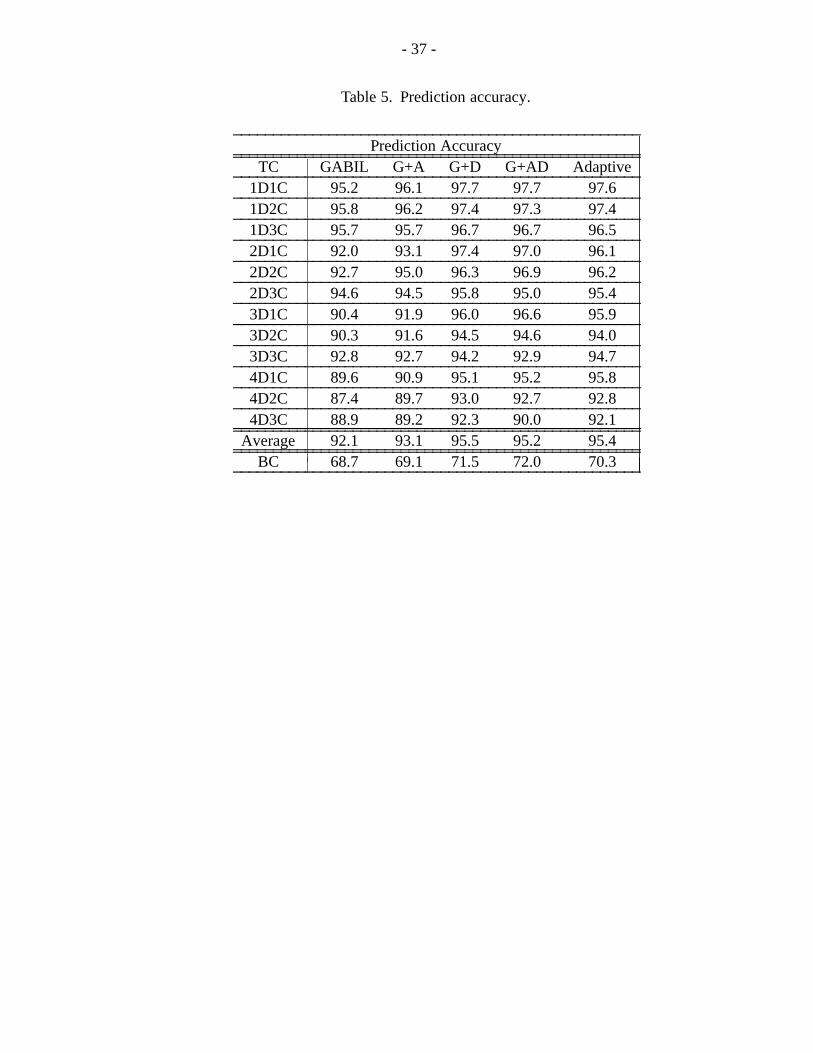
- 37 -


___________________________________________________Prediction Accuracy______________________________________________________________________________________________________

TC GABIL G+A G+D G+AD Adaptive___________________________________________________1D1C 95.2 96.1 97.7 97.7 97.6___________________________________________________1D2C 95.8 96.2 97.4 97.3 97.4___________________________________________________1D3C 95.7 95.7 96.7 96.7 96.5___________________________________________________2D1C 92.0 93.1 97.4 97.0 96.1___________________________________________________2D2C 92.7 95.0 96.3 96.9 96.2___________________________________________________2D3C 94.6 94.5 95.8 95.0 95.4___________________________________________________3D1C 90.4 91.9 96.0 96.6 95.9___________________________________________________3D2C 90.3 91.6 94.5 94.6 94.0___________________________________________________3D3C 92.8 92.7 94.2 92.9 94.7___________________________________________________4D1C 89.6 90.9 95.1 95.2 95.8___________________________________________________4D2C 87.4 89.7 93.0 92.7 92.8___________________________________________________4D3C 88.9 89.2 92.3 90.0 92.1______________________________________________________________________________________________________

Average 92.1 93.1 95.5 95.2 95.4______________________________________________________________________________________________________BC 68.7 69.1 71.5 72.0 70.3___________________________________________________

��

��

��

- 38 -


_______________________________________________Convergence______________________________________________________________________________________________

TC GABIL G+A G+D G+AD Adaptive_______________________________________________1D1C 87 58 28 32 34_______________________________________________1D2C 100 85 59 68 58_______________________________________________1D3C 96 97 94 97 97_______________________________________________2D1C 109 90 42 42 50_______________________________________________2D2C 148 93 82 55 80_______________________________________________2D3C 249 250 136 250 120_______________________________________________3D1C 103 104 54 39 53_______________________________________________3D2C 125 127 76 62 70_______________________________________________3D3C 225 240 161 240 128_______________________________________________4D1C 131 120 67 62 55_______________________________________________4D2C 142 133 75 75 80_______________________________________________4D3C 229 253 166 248 130______________________________________________________________________________________________

Average 145 138 87 106 80_______________________________________________��

��

��

- 39 -

Table 7. Comparison of system characteristics.

___________________________________________________________System Bias Space Searches GA______________________________________________________________________________________________________________________

CRL/ISO hypothesis selection criteria uncoupled noprediction strategy___________________________________________________________

ClimBS beam width uncoupled nohypothesis coverage___________________________________________________________

PEAK learning strategy uncoupled no___________________________________________________________VBMS concept learners uncoupled no___________________________________________________________

GIL generalization operators uncoupled yes___________________________________________________________Adaptive GABIL generalization operators coupled yes___________________________________________________________

��

��

��

��

��

- 40 -

Table 8. Predictive Accuracy on nDmC.

_______________________System Sig Wins______________________________________________AQ14 80% No_______________________C4.5P 80% Yes_______________________C4.5U < 80% No_______________________ID5R < 80% Yes_______________________IACL 80% Yes_______________________

GABIL 95% Yes_______________________G+A 95% Yes_______________________G+D < 80% No_______________________

G+AD < 80% Yes_______________________��

��

��

��

- 41 -

Table 9. Convergence on nDmC.

_______________________System Sig Wins______________________________________________AQ14 < 80% No_______________________C4.5P 95% Yes_______________________C4.5U < 80% Tie_______________________ID5R < 80% Yes_______________________IACL 95% Yes_______________________

GABIL 95% Yes_______________________G+A 95% Yes_______________________G+D < 80% Yes_______________________

G+AD < 80% Yes_______________________��

��

��

��

- 42 -

Table 10. Predictive Accuracy on BC.

_____________________System Sig Wins__________________________________________AQ14 95% Yes_____________________C4.5P 95% No_____________________C4.5U 95% Yes_____________________ID5R 95% Yes_____________________IACL 95% Yes_____________________

GABIL 90% Yes_____________________G+A 80% Yes_____________________G+D 80% No_____________________

G+AD 95% No_____________________��

��

��

��

using genetic algorithms for concept learningbylander/cs6243/dejong1993genetic.pdf ·...

Documents