El-Naggar, A. G., Hedley, C. B, Horne D, Roudier P, Clothier B, 2017. Using electrical conductivity imaging to estimate soil water content. In: Science and policy: nutrient management challenges for the next generation. (Eds L. D. Currie and M. J. Hedley). http://flrc.massey.ac.nz/publications.html. Occasional Report No. 30. Fertilizer and Lime Research Centre, Massey University, Palmerston North, New Zealand. 13 pages.

1

USING ELECTRICAL CONDUCTIVITY IMAGING TO ESTIMATE

SOIL WATER CONTENT

Ahmed El-Naggar1, Carolyn Hedley2, David Horne1, Pierre Roudier2, Brent Clothier3

1 Institute of Agriculture and Environment, Massey University, Palmerston North, New Zealand

2 Landcare Research, Riddet Road, Massey University Campus, Palmerston North 4442 3 Plant & Food Research, Batchelar Road, Palmerston North 4442

Abstract

Measurement of volumetric soil water content (θv cm3 cm

-3) requires collection and analysis

of soil samples, which is expensive and time consuming, or soil moisture sensing, which is

limited spatially by the number of sensors installed. Apparent electrical conductivity (ECa) of

the soil profile can be used as an indicator of a number of soil properties, including soil

moisture. Therefore, ECa sensor surveys can be used to efficiently and inexpensively predict

θv along a transect or across a field.

In this study, EM4Soil inversion software was used to generate: (i) two-dimensional depth

profile models of electrical conductivity (ECa, mSm-1

) as measured by a multi-coil

DUALEM-421S sensor and a DUALEM 1s sensor, and (ii) a correlation between the

calculated conductivity profiles and the measured θv.

ECa survey data were collected along two transects (12 positions) and 8 randomly stratified

positions in a field near Palmerston North. Soil samples were taken at 0.30 m increments to a

depth of 1.5 m. The θv of these samples was determined in the laboratory. The appropriate

calibration between ECa and θv was achieved using inversion parameters of forward

modelling, an inversion algorithm and a damping factor. In general, the results show that θv

and ECa follow similar trends down the soil profile. Reasonably accurate relationships

between ECa and θv were determined using a ‘leave-one-out’ cross validation approach (R2 =

0.62 for DUALEM-421S and 0.58 for DUALEM 1s). The cross validation equation for the

predicted versus measured θv for 99 samples has a good R2 (0.62 for DUALEM-421S and

0.58 for DUALEM 1s) and a small RMSE (0.04 cm3cm

-3 for DUALEM-421S and 0.04

cm3cm

-3 for DUALEM 1s). We conclude that soil ECa can be used to indirectly estimate (θv)

if the predictive power of the ECa for θv is moderated by other soil factors that also affect the

EC sensors. For example, if clay content were uniform across the whole, then EC would relate

more closely to θv.

Introduction Agriculture is the biggest water user, with irrigation accounting for approximately 70 percent

of all the freshwater withdrawn in the world. Without improved efficiencies, agricultural

water consumption is expected to increase globally by about 20% by 2050 (UN water, 2014).

Variations in water availability across a field due to different soil characteristics or crop needs

may require site-specific irrigation management to achieve optimum yields and maximize

water use efficiency.

2

To identify the irrigation management zones based on varying soil characteristics an

electromagnetic (EM) survey can be used. Electromagnetic sensors measure the apparent soil

electrical conductivity (ECa, mSm-1

), which has been shown to be influenced by various soil

(e.g. clay and mineralogy) and hydrological properties (e.g. moisture) (Triantafilis et al.,

2013).

The DUALEM-421 incorporates an EM transmitter that operated at a fixed low frequency (9

kHz) and 3 pairs of horizontal co-planar (HCP) and perpendicular (PRP) receiver arrays. The

depth of ECa measurement is, respectively, 0–1.5 (1mHcon), 0–3.0 (2mHcon) and 0–6.0 m

(4mHcon), and 1.1, 2.1 and 4.1 m (PRP) (Triantafilis & Santos, 2013). The DUALEM-1 has

1-m separation between its transmitter and dual receivers, so its dual depths of conductivity

measurement are 0.5 m and 1.5 m. Site investigation is essential to check which factors are

influencing the soil electrical conductivity. In much of New Zealand, EM variation indicates

variations in soil texture and moisture.

If there is one varying feature, such as percent stones, then a relationship can be developed to

predict AWC directly from EC. Also if there is no simple relationship between EC and soil

variability (e.g. different soil layering) then a zone-specific AWC can be assigned to each

zone. A soil AWC map is useful information for managing any type of irrigation system. It

allows irrigation managers to zone paddocks for different management, and to place soil

moisture measurement equipment with knowledge of lighter or heavier soil types (Hedley et

al., 2009).

Triantafilis and Monteiro Santos (2009) illustrated that EM4Soil software can be used to

invert single frequency (EM38 and EM31) and multiple coil arrayed DUALEM-421 to

produce a map of exchangeable sodium percentage (Huang et al., 2014) and clay (Triantafilis

et al., 2013).

Our current study focusses on (i) using EM4Soil inversion software to generate a two-

dimensional depth profile model of electrical conductivity (ECa, mSm-1

) measured by single

and multi-coil EM sensor surveys, and (ii) developing a correlation relationship between the

calculated vertical profile of conductivity with the measured volumetric moisture content (θv,

cm3 cm

-3).

Method

Study site

The study field is located in Palmerston North, New Zealand, at Massey University (lat.

40°22′57.4″S, long. 175°35′38.2″E). The study field is 4 ha and was cultivated and sown with

Ryegrass (Lolium perenne L.) and clover. The soils are classified as Fluvial Recent soils

formed in greywacke alluvium (Pollok et al., 2003; Hewitt 1998).

3

Fig.1. Study area location, EM survey transect soil sampling locations (Mnfsl: Manawatu

fine sandy loam, Mnsil/s: Manawatu silt loam over sand, Mnsl: Manawatu sandy loam) {Pollok, J.A., Nelson, P.,

Touhy, M.P., Gillingham, S.S., Alexander, M., 2003 Massey University Soil Map.

http://atlas.massey.ac.nz/soils/index_soils.asp}

EM survey (DUALEM-421S and DUALEM-1S), soil sampling and laboratory analysis

The EM survey and collection of ECa data along 2 transects was carried out at a height of

0.25 m (DUALEM-1S) and 0.15 m (DUALEM-421S). To calibrate the inverted ECa data, the

calibration sites were selected as shown in Fig 1. On transects 1 and 2, 6 soil samples sites

were selected. On transects 1, soil samples were collected at 15.6 m intervals while on

transect 2 were at 17 m intervals. At each site, soil samples were taken at 0.30 m to a depth of

1.5m. Sampling was carried out on the same data that the ECa data was acquired

(22/09/2016). Laboratory analysis included measurements of gravimetric water soil water

content (θg, gg-1

) on an oven dry-weight basis and these calculations were then converted to

volumetric soil water content (θv, cm3cm

-3) by multiplication with the soil bulk density as in

equation: θv = (pb)/(pw) x θg where pw is the density of water (g cm-3) (Gardner, 1986).

EM4Soil and 2D inversion of ECa data

EM4Soil is a software package (EMTOMO, 2013) which was developed in order to invert

ECa data acquired at low induction numbers. The algorithm is described by Monteiro Santos

et al. (2010).

In this study, the forward modelling is based upon the cumulative function (CF) (McNeill,

1980; Wait, 1962). The so called ‘full-solution’ of EM fields (FS) (Kaufman and Keller,

1983) is also calculated by the model (results not shown). The modelling is conducted using a

1-dimensional laterally constrained approach (Auken et al., 2002), where 2-dimensional

smoothness constraints are imposed. The inversion algorithms (S1 and S2) are based upon the

Occam regularization method (e.g. DeGroot and Constable 1990; Sasaki 1989). The latter

constrains electromagnetic conductivity images (EMCI) variation around a reference model

and is smoother than S1.

4

For running EM4Soil, a smoothing or damping factor (λ) is required. A large value of λ will

achieve a very smooth model where λ leads to equilibrium between data misfit and

smoothness of the EMCI model (Triantafilis et al., 2013). In this study, we used the FS

model, S2 algorithm and λ = 0.04. Inversion of ECa was generated with a maximum of 10

iterations. We calculated ECa (σ) using an initial model (σ = 35 mSm-1

).

Estimating the soil water content and validation of prediction accuracy

A liner regression was used for developing the calibration relationship between ECa and θv

data. This regression model was then validated using a ‘leave-one-group-out’ cross-validation

approach. In this case, the model is repeatedly refit leaving out a single observation and then

used to derive a prediction for the left-out observation. Within the literature, it is widely

appreciated that ‘leave-one-out’ is a suboptimal method for cross-validation, as it gives

estimates of the prediction error that are more variable than other forms of cross validation

and it is a useful and appropriate method for relatively small datasets, such as this one.

(Friedman et al., 2001)

The predictive power of the model is described by the average R2 and RMSE determined

from the cross validation process.

Results

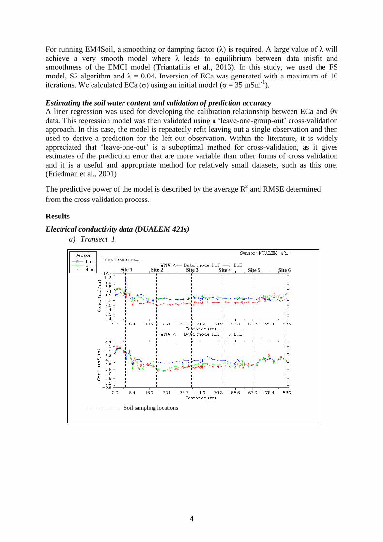
Electrical conductivity data (DUALEM 421s)

a) Transect 1

Site 1 Site 2 Site 3 Site 4 Site 5 Site 6

Soil sampling locations

5

b) Transect 2

Fig.2. Measured apparent soil electrical conductivity (ECa, mSm

-1) along transect

1 and 2 using the DUALEM-421 sensor in horizontal coplanar (Hcon) and

perpendicular coplanar (Pcon) for spacing (a) 1, (b) 2 and, (c) 4 m

Electrical conductivity data (DUALEM 1s)

a) Transect 1

Soil sampling locations

Site 1 Site 2 Site 3 Site 4 Site 5 Site 6

Site 1 Site 2 Site 3 Site 4 Site 5 Site 6

Soil sampling locations

6

b) Transect 2

Fig.3. Measured apparent soil electrical conductivity (ECa, mSm-1

) along transect 1 and

2 using the DUALEM1S sensor in horizontal coplanar (Hcon) and perpendicular

coplanar (Pcon) for spacing 1m

2-D depth profile modelling of electromagnetic conductivity

a) Transect 1

Site 1 Site 2 Site 3 Site 4 Site 5 Site 6

Soil sampling locations

DUALEM421

S

7

b) Transect 2

Fig.4. Vertical conductivity profiles derived from the Q2D (quantitative 2D) model for the

two transects

DUALEM1S

DUALEM1S

DUALEM421

S

8

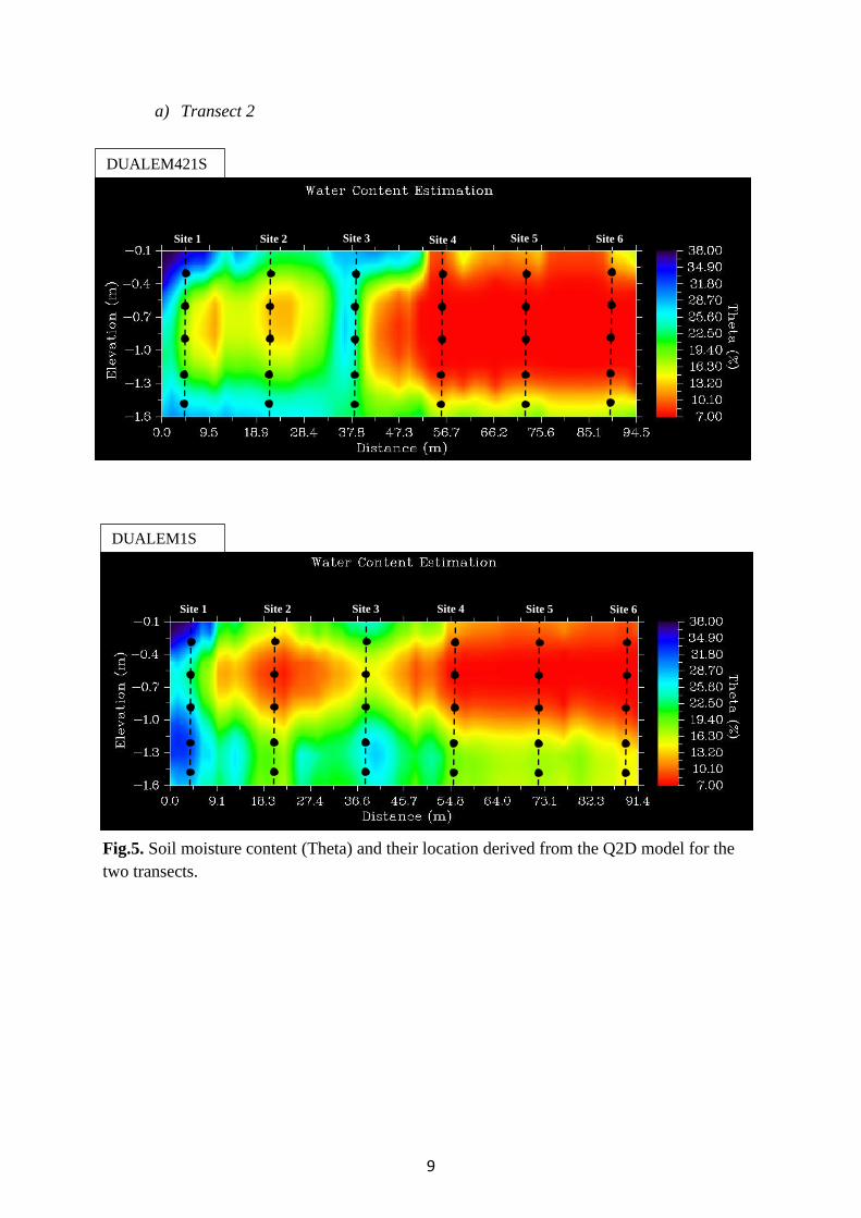
2-D depth profile modelling of predicted soil moisture (cm3, cm

-3) content along two

transects

a) Transect 1

DUALEM421S

DUALEM1S

Site 1 Site 2 Site 3 Site 4 Site 5 Site 6

Site 1 Site 2 Site 3 Site 4 Site 5 Site 6

9

a) Transect 2

Fig.5. Soil moisture content (Theta) and their location derived from the Q2D model for the

two transects.

DUALEM421S

DUALEM1S

Site 1 Site 2 Site 3 Site 4 Site 5 Site 6

Site 1 Site 2 Site 3 Site 4 Site 5 Site 6

10

Measured θv and ECa data at specific depths

a)

b)

Fig.6. a) Volumetric soil content (θv, cm3cm

-3) and estimated soil electrical conductivity

(ECa, mSm-1

) values for position 2 and position 20 measured in the lab at 5 depths (a)

DUALEM-421s (b) DUALEM-1S

11

y = 0.6287x + 0.0633 R² = 0.62

RMSE = 0.04

0

0.05

0.1

0.15

0.2

0.25

0.3

0.35

0.4

0 0.1 0.2 0.3 0.4

Esti

mat

ed

θv(

cm3 c

m-3

)

Measured θv(cm3cm-3)

Validation of estimated θv (cm3cm

-3)

a) DUALEM421s

Fig.7. Predicted soil water content (θv, cm3cm

-3) derived from electrical

conductivity (DUALEM-421S) versus measured soil water content (θv,

cm3cm

-3).

b) DUALEM1S

Fig.8. Predicted soil water content (θv, cm

3cm

-3) derived from electrical

conductivity (DUALEM-1S) versus measured soil water content (θv, cm3cm

-3).

Discussion

Fig.2 and Fig.3 are showing the ECa values for three DOE (depths of exploration) obtained

using the three coil system (DUALEM-421) and one DOE for the one coil system

(DUALEM-1S) for transect 1 and transect 2, respectively. The average values of the

DUALEM-421S ECa data for 1m Pcon and 1m Hcon = 3.3 mSm-1

(exploration depth 0.5 and

1.5 m respectively) and are slightly higher than for 2m Pcon = 3.1 mSm-1

(exploration depth 1

m). Similarly, the DUALEM-1S ECa data shows the average values of 1m Pcon (exploration

depth 0.5m) = 21.9 mSm-1

which are higher than for 1m Hcon (exploration depth 1.5m) = 3.1

y = 0.5057x + 0.081 R² = 0.58

RMSE = 0.05

0

0.05

0.1

0.15

0.2

0.25

0.3

0 0.1 0.2 0.3 0.4

Esti

mat

ed

θv(

cm3 c

m-3

)

Measured θv(cm3cm-3)

12

mSm-1

. This suggests a slightly higher conductor in the topsoil and the deep subsoil (0-0.5m

and 1-1.5m) than subsoil (0.5-1m). Transect 2 ECa values started higher then decrease

rapidly to north which suggests that transect 2 is located in a contrasting soil (texture).

Decreasing ECa values are likely to indicate a coarser and/or drier soil, and investigation of

the soil map (Pollok et al., 2003) showed that this area of soils is sandier (see Fig.1) also the

lab measurements of θv were lower in this area which relates to the coarser textured soil type.

Fig.4 shows 2-D maps of vertical conductivity profiles derived from the Q2D model. ECa

values are higher in the top soil then decrease in the subsoil then increase into the deep

subsoil and this indicates the impact of wetness and/or soil texture. The inverted ECa values

show two distinct regions for transect 2 which relate to the two different soil types (see Fig.

1). We attribute that the last two positions located in a Manawatu sandy loam soil as

described by a previous investigation (Pollok et al., 2003). The ECa values show a similar

trend to soil moisture data so that a relationship between ECa and θv has been established at

this field site.

Fig.5 shows the 2-D map of estimated soil water content along transect 1 and 2 using the

inverted ECa data at different depths. One important observation is that there is an over

estimated value for θv for the topsoil at the first location (5m), and we attributed this to an

elevated ECa value due to soil compaction, where a higher bulk density value was recorded. It

is suggested that the topsoil has a high value of θv which then decreases in the subsoil and

then increases into the deeper subsoil which gives a quite similar indication to our soil

moisture data.

Fig.6 (a, b) shows the results of volumetric soil water content (θv, cm3cm

-3) and estimated soil

electrical conductivity (ECa, mSm-1

) for positions 2 and 20 at 5 depths (0-30, 30-60, 60-90,

90-120, and 120-150). Our result indicates that θv and ECa follow similar trends down soil

profiles. The trends of soil moisture to the subsoil (0.6-0.9m) decreases then increases into the

shallow subsoil (0.9-1.5m) in positions (P1, P3, P6, P8) while in P2 it starts increasing from

0.6 to 1.5m (results only shown for P2 and P20). There is a fluctuation in the soil moisture

trend in P4, P7, P5 and P10 where in P4 and P7 it increases to the subsoil (0.6-0.9m) then

decreases form (0.9-1.2m) then increase again into the shallow subsoil (1.2-1.5m) while it

decreases suddenly in P2 (due to stone contents where the sample was taken into 0.9-1.33m

due to finding stones layer>1.30m) and slightly decreases in P10. In general, these findings

suggest these ECa variations relate to variations in soil layering and soil type.

A leave-one-out cross validation approach was used to correlate the estimated ECa (mSm-1

)

and measured θv (cm3cm

-3) and it indicates a good average R

2 (0.62 for DUALEM-421S and

0.58 for DUALEM 1s) and a small RMSE (0.04 cm3cm

-3 for DUALEM-421S and 0.04

cm3cm

-3 for DUALEM 1s) (Fig.7 and Fig.8).

Conclusion The inversion model (EM4soil) has been shown to be a useful tool for mapping ECa (mSm

-1)

which is then related to measured θv (cm3cm

-3). This can assist in irrigation management as

explained below. The inversion method estimates ECa (mSm-1

) at specific depths which are

then used to produce (i) a 2-D ECa map and (ii) by establishing a correlation between ECa

(mSm-1

) and θv (cm3cm

-3), it can be used to produce a 2-D soil moisture depth profile map.

This map gives an indication about the areas at higher risk to deep drainage (i.e. the wetter

zones), the spatial variability of soil moisture at different layers and this guided placement of

soil moisture sensors into the field. Integrating the EM data as a reasonable tool for

13

representing the spatial variability of the soil with soil moisture sensors data (temporal change

in θv) could be useful in improving irrigation management. Future work could be developing

a calibration between ECa, particle size and CEC.

References

Amidu, S. A. and J. A. Dunbar (2007). "Geoelectric studies of seasonal wetting and drying of a Texas

Vertisol." Vadose Zone Journal 6(3): 511-523.

Auken, E., Foged, N., Sorensen, K.I., 2002. Model recognition by 1-D laterallyconstrained inversion

of resistivity data. In: Matias, M.S., Grangeia, C. (Eds.),Proceedings of 8th Meeting Environmental

and Engineering Geophysics,EEGS-ES. University of Aveiro Portugal, pp. 241–244.

deGroot-Hedlin, C. and S. Constable (1990). "Occam's inversion to generate smooth, two-dimensional

models from magnetotelluric data." Geophysics 55(12): 1613-1624.

Friedman, J., T. Hastie, et al. (2001). The elements of statistical learning, Springer series in statistics

Springer, Berlin.

EMTOMO, 2014. EM4Soil Version 2. EMTOMO, R. Alice Cruz 4, Odivelas, Lisboa,Portugal.

Gardner, W.H. 1986. Water Content. In Methods of Soil Analysis. Part I. Physical and Mineralogical

Methods (Klute, A., ed.). Agronomy Series No 9. 2nd ed, pp.493-544. ASA

Madison WI.

Hedley, C. B. and I. J. Yule (2009). "Soil water status mapping and two variable-rate irrigation

scenarios." Precision Agriculture 10(4): 342-355.

Huang, J., G. Davies, et al. (2014). "Spatial prediction of the exchangeable sodium percentage at

multiple depths using electromagnetic inversion modelling." Soil use and management 30(2): 241-

250.

Kaufman, A. A. and G. V. Keller (1983). Frequency and transient soundings, Springer.

McNeill, J. (1980). Electromagnetic terrain conductivity measurement at low induction numbers,

Geonics Limited Ontario, Canada.

Monteiro Santos, FA, Triantafilis, J., Taylor, R., Holladay, S. and Bruzgulis, K., 2010. Inversion of

conductivity profiles using full solution and a 1-D laterally constrained algorithm. Journal of

Environmental and Engineering Geophysics, 15, 3, 163-174.

Sasaki Y., 1989. Two-dimensional joint inversion of magnetotelluric and dipole-dipole resistivity data.

Geophysics, 54, 254-262.

Triantafilis, J. and F. M. Santos (2010). "2-dimensional soil and vadose-zone representation using an

EM38 and EM34 and a laterally constrained inversion model." Soil Research 47(8): 809-820.

Triantafilis, J., C. Terhune, et al. (2013). "An inversion approach to generate electromagnetic

conductivity images from signal data." Environmental modelling & software 43: 88-95.

Wait, J.R. 1962. A note on the electromagnetic response of a stratified earth. Geophysics 27:382–385.

UN Water (2014). http://www.unwater.org