This paper has not been DEST reviewed

Using decision trees to provide rapid estimates of earthquake loss

Bridget Ayling1, Trevor Dhu2, Ken Dale3, Ole Nielsen4

1 Geothermal Energy Project, Onshore Energy and Minerals Division, Geoscience Australia, GPO Box 378, Canberra, ACT 2601, Australia 2 Natural Hazard Impacts Project, Geospatial and Earth Monitoring Division, Geoscience Australia, GPO Box 378, Canberra, ACT 2601, Australia 3 Engineering and Vulnerability Project, Geospatial and Earth Monitoring Division, Geoscience Australia, GPO Box 378, Canberra, ACT 2601, Australia 4 Natural Hazard Impacts Project, Geospatial and Earth Monitoring Division, Geoscience Australia, GPO Box 378, Canberra, ACT 2601, Australia

Abstract

The ability to provide rapid, accurate estimates of damage following a large earthquake event is critical for effective disaster response. At Geoscience Australia, an engineering approach is used to model ground motion, the associated structural damage and loss, utilizing the capacity spectrum method (CSM) to estimate structural damage. The iterative nature of the CSM requires proportionally more computing time, thus slowing the speed at which total loss estimates can be generated. In this study, an alternative approach is explored that is still based on the CSM but is not iterative, instead using decision trees to predict loss for a given earthquake and building type. The basis for these decision trees lie in a data-mining process, whereby a synthetic earthquake catalogue was generated that incorporated multiple earthquake scenarios (i.e.: sequentially varying earthquake magnitude, ground motion model, site location and building type) on the same fault (simulated as the Newcastle fault), with loss calculated for each event. CART (Classification and Regression Tree) software was used to generate building-specific decision trees, and the predictive accuracy of these trees was tested on selected building types using independent test datasets. The variable found to be most important in splitting the dataset (the best predictor of loss) for each building type was always a particular period of ground motion in the earthquake response spectra. This period was also found to be logarithmically related to the elastic period for the given building type. It was found decisions trees were able to produce aggregated loss estimates within 6% of the estimate generated using the CSM for earthquakes greater than magnitude 6 and using the Toro, Sadigh or Allen ground motion model. If implemented, the increased computational efficiency of the decision-tree approach would enable rapid generation of loss estimates following an earthquake event, and sampling of more earthquakes for probabilistic seismic risk analysis (PSRA) to generate a better understanding of earthquake risk in Australia.

Keywords: structural damage, capacity spectrum method, data mining, decision trees, elastic period, financial loss 1. INTRODUCTION The ability to provide rapid and accurate estimates of damage following an earthquake is a key priority in seismic risk research, and is central to efficient disaster management. Internationally, several groups are dedicated to achieving these rapid earthquake loss estimates, including SAFER (Seismic eArly warning For EuRope), WAPMERR (World Agency of Planetary Monitoring and Earthquake Risk Reduction) and the automated alarm system ‘PAGER’ (Prompt Assessment of Global Earthquakes for Response) being developed by the USGS. These agencies aim to provide real-time loss estimates following earthquake events using an empirical approach: historical earthquake data are used to estimate building fragilities, i.e. the relationship between ground shaking intensity and observed structural damage to buildings, which are then used in conjunction with maps of shaking intensity (shake maps) to provide loss estimates. In Australia, this approach is not practicable as there are few historical examples of large, damaging earthquakes in populated areas that can be used as benchmarks for loss estimates. At Geoscience Australia, probabilistic seismic risk analysis (PSRA: the direct financial loss and its likelihood of occurrence) and probabilistic seismic hazard analysis (PSHA: the ground motion and its likelihood of occurrence) are calculated through an engineering-based approach, using a Matlab-based computer application known as EQRM (EarthQuake Risk Model) (Robinson et al., 2005). The process used to generate earthquake hazard and risk estimates is initially identical, beginning with the generation of a synthetic earthquake catalogue, modelling of the associated ground motion and probability of occurrence, use of an attenuation model to describe the propagation of seismic waves to the locations of interest, and finally, incorporation of a site-response model to account for effects of local regolith & geology. However PSRA incorporates additional steps: (1) estimation of the probability that a building portfolio will experience different levels of damage; (2) computation of the direct financial loss as a result of these probabilities; and (3) aggregation of these losses and estimation of probability of their exceedance to produce a risk value (Patchett et al., 2005, Robinson et al., 2005). Step 1 utilises a method known as the Capacity Spectrum Method (hereafter CSM), an approach that compares the capacity of a structure (in the form of a pushover curve) with the demands on a structure (the earthquake response spectra; Freeman (2004)). The graphical intersection of the capacity curve, and iteratively modified demand curve, provide an estimate of the building’s peak response displacement and acceleration (Freeman, 2004; Kircher et al., 2005). These in turn are used with fragility curves to estimate probabilities that the building experiences different levels of damage for three components of the building – the displacement sensitive structural system, the displacement sensitive non-structural system and the acceleration sensitive non-structural elements. From the damage probabilities, total and percentage loss are calculated using a financial loss model. Percentage loss is defined as the repair cost divided by the total replacement value. Owing to its iterative nature, the CSM is the most computationally-intensive step in the PSRA calculation. The goal of this study was to investigate using decision trees as an alternative approach to predicting financial loss from an earthquake, which may be faster and of comparable accuracy to the CSM. The proposed approach is still based on the CSM (the CSM is used to create a synthetic loss dataset), however decision tree rules that are generated

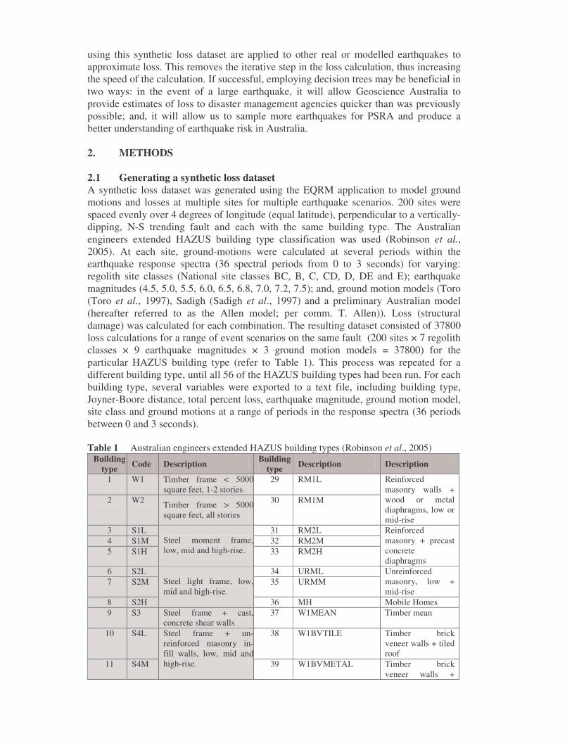
using this synthetic loss dataset are applied to other real or modelled earthquakes to approximate loss. This removes the iterative step in the loss calculation, thus increasing the speed of the calculation. If successful, employing decision trees may be beneficial in two ways: in the event of a large earthquake, it will allow Geoscience Australia to provide estimates of loss to disaster management agencies quicker than was previously possible; and, it will allow us to sample more earthquakes for PSRA and produce a better understanding of earthquake risk in Australia. 2. METHODS 2.1 Generating a synthetic loss dataset A synthetic loss dataset was generated using the EQRM application to model ground motions and losses at multiple sites for multiple earthquake scenarios. 200 sites were spaced evenly over 4 degrees of longitude (equal latitude), perpendicular to a vertically-dipping, N-S trending fault and each with the same building type. The Australian engineers extended HAZUS building type classification was used (Robinson et al., 2005). At each site, ground-motions were calculated at several periods within the earthquake response spectra (36 spectral periods from 0 to 3 seconds) for varying: regolith site classes (National site classes BC, B, C, CD, D, DE and E); earthquake magnitudes (4.5, 5.0, 5.5, 6.0, 6.5, 6.8, 7.0, 7.2, 7.5); and, ground motion models (Toro (Toro et al., 1997), Sadigh (Sadigh et al., 1997) and a preliminary Australian model (hereafter referred to as the Allen model; per comm. T. Allen)). Loss (structural damage) was calculated for each combination. The resulting dataset consisted of 37800 loss calculations for a range of event scenarios on the same fault (200 sites × 7 regolith classes × 9 earthquake magnitudes × 3 ground motion models = 37800) for the particular HAZUS building type (refer to Table 1). This process was repeated for a different building type, until all 56 of the HAZUS building types had been run. For each building type, several variables were exported to a text file, including building type, Joyner-Boore distance, total percent loss, earthquake magnitude, ground motion model, site class and ground motions at a range of periods in the response spectra (36 periods between 0 and 3 seconds). Table 1 Australian engineers extended HAZUS building types (Robinson et al., 2005)

Building type Code Description Building

type Description Description

1 W1 Timber frame < 5000 square feet, 1-2 stories

29 RM1L

2 W2 Timber frame > 5000 square feet, all stories

30 RM1M

Reinforced masonry walls + wood or metal diaphragms, low or mid-rise

3 S1L 31 RM2L 4 S1M 32 RM2M 5 S1H

Steel moment frame, low, mid and high-rise. 33 RM2H

Reinforced masonry + precast concrete diaphragms

6 S2L 34 URML 7 S2M 35 URMM

Unreinforced masonry, low + mid-rise

8 S2H

Steel light frame, low, mid and high-rise.

36 MH Mobile Homes 9 S3 Steel frame + cast,

concrete shear walls 37 W1MEAN Timber mean

10 S4L 38 W1BVTILE Timber brick veneer walls + tiled roof

11 S4M

Steel frame + un-reinforced masonry in-fill walls, low, mid and high-rise. 39 W1BVMETAL Timber brick

veneer walls +

metal roof 12 S4H 40 W1TIMBERTILE Timber walls +

tiled roof 13 S5L 41 W1TIMBERMETAL Timber walls +

metal roof 14 S5M 42 C1LMEAN Concrete moment

frame, low-rise, mean

15 S5H

Steel frame + concrete shear walls, low, mid and high-rise.

43 C1LSOFT Concrete moment frame, low-rise, soft-story

16 C1L 44 C1LNOSFT Concrete moment frame, low-rise, non-soft-story

17 C1M 45 C1MMEAN Concrete moment frame, mean

18 C1H

Concrete moment frame

46 C1MSOFT Concrete moment frame, mid-rise, soft-story

19 C2L 47 C1MNOSOFT Concrete moment frame, mid-rise, non-soft-story

20 C2M 48 C1HMEAN Concrete moment frame high-rise

21 C2H

Concrete shear walls, low, mid and high-rise.

49 C1HSOFT Concrete moment frame, high-rise, soft-story

22 C3L 50 C1HNOSOFT Concrete moment frame, high-rise, non-soft-story

23 C3M 51 URMLMEAN Unreinforced masonry, low-rise, mean

24 C3H

Concrete frame + un-reinforced masonry in-fill walls, low, mid and high-rise.

52 URMLTILE Unreinforced masonry, low-rise, tile roof

25 PC1 Precast concrete tilt-up walls

53 URMLMETAL Unreinforced masonry, low-rise, metal roof

26 PC2L 54 URMMMEAN Unreinforced masonry, mid-rise, mean

27 PC2M

55 URMMTILE Unreinforced masonry, mid-rise, tile roof

28 PC2H

Precast concrete frames with concrete shear walls, low, mid and high-rise.

56 URMMMETAL Unreinforced masonry, mid-rise, metal roof

2.2 CART (Classification and Regression Tree Analysis) CART is a software package that builds classification and regression trees for predicting continuous variables (regression) and categorical variables (classification). The rationale for using CART was: (a) to find which variables appear most important in determining structural damage (loss); and (b) to generate a decision tree (rules) using these variables and their values, which will allow us to predict loss. Advantages of using CART are that it is non-parametric, and can evaluate data that are highly-skewed or multimodal (Lewis, 2000). In addition, it is well suited for data-mining in that it can reveal non-obvious, complex relationships between the splitting variables and the predicted variable.

CART analysis involves four steps: (1) tree building (2) end of tree building (3) tree ‘pruning’ (4) optimal tree selection. These steps are discussed in further detail as follows: (1) Tree-building begins at the root node, and CART finds the best possible variable to

split the node into two child nodes, based on an exhaustive search of all possibilities of splitter variables and the values of the variable to be used to split the node. These child nodes are then split and so forth.

(2) Splitting stops when there is only one data-point left in each node, or when all data-points in a node are the same. The point at which this splitting stops is called the ‘maximal tree’. This tree often ‘overfits’ the data, because it follows every idiosyncrasy in the dataset that may not occur in another, independent dataset.

(3) In tree pruning, the method of ‘cost complexity’ (a measure of how much additional accuracy a split will add to the entire tree vs. the extra tree complexity) is used to prune child nodes from the maximal tree.

(4) ‘Optimal tree’ selection is performed by cross validating the dataset. This is done by applying the maximal tree created from one set of observations (learning data), to an independent set of data (test data) to determine its predictive accuracy. The point where the tree begins to overfit the learning data (i.e. starts to follow the idiosyncrasies of the data vs. general trends) is found where the predictive accuracy of the tree begins to decrease (this is the optimal tree).

The purpose of generating a decision tree for this study was to enable the accurate prediction of loss percentage using the value of certain predictor variables. In order to achieve this, we first needed to establish which variables were statistically most important in determining percent loss. To do this, percent loss was selected as the target variable (the variable we hope to predict), and the following variables were selected as potential predictor variables (splitting variables): earthquake magnitude, ground motion model, regolith site class, distance, and ground motions at 36 spectral periods (from 0 secs through to 3 secs). 30% of the input data was selected at random for cross-validation of the tree. As the input variables were mainly continuous, CART was run in regression-tree mode. The output of this process was a rank, indicating relative importance of these predictors. To avoid having up to 40 potential predictor variables, the next step was to run the regression-tree analysis again with the highest-ranked predictors (1,2,3), and assess the relative accuracy and size of the optimal tree. Criteria imposed on this process were as follows:

� A minimum of 5 data-points per terminal node; � Less than 100 terminal nodes in final decision tree ; � Absolute within-node variability less than 10%, and ideally less than 5% (this

affects the ability of the tree to accurately predict percent loss values within 5 or 10%) (Figure 1); and

� The tree was independently tested using 30% of the learning dataset (cross-validation (CV)): the optimal tree is found where maximum predictive accuracy of the tree is observed (corresponds to the minimum CV cost).

Frequently, the optimal tree had in excess of 100 terminal nodes. In this case, ‘best-trees’ were selected using an automatic tree-pruning procedure that chooses a smaller

Figure 1 Terminal nodes sorted by target variable prediction (percent loss), illustrating (A) good tree-building with low within-node variability (Building type 50, 1SE rule, 3 predictors, 44 terminal nodes), and (B) poor tree building with multiple nodes overlapping in values and with large within-node variability (Building type 41, 1SE rule, 2 predictors, 48 terminal nodes). tree with CV costs that are not much greater than the minimum CV cost (optimal tree). This automated pruning uses a standard error (SE) rule, for example by applying a 1 SE rule, a tree will be chosen that has a CV cost not greater than the minimum CV cost + 1 SE of the CV cost. After selecting the ‘best tree’ (with 3 or less predictor variables, less than 100 terminal nodes and a relative error close to that at the optimal tree), a final test of the predictive power of the trees was performed. On selected building types (HAZUS types 1,6,11,16,21,26 etc up to 56), a second raw dataset was generated using EQRM for different earthquake magnitudes than those in the learning dataset (earthquake magnitudes 4.7, 5.2, 5.7, 6.2, 6.6, 6.9, 7.1, 7.4). Applying the ‘best trees’ to these datasets provides an indication of the total predictive accuracy of the decision trees. This was always smaller than 0.5 RMS error for the whole tree, indicating that the tree-building methodology is robust. For each node, a mean value and standard deviation is given, and for the best-tree selected for each building type, these values were extracted into a table to be used later in the rule implementation (discussed below). 2.3 Rule generation and implementation

A

B

In CART, the rules for each terminal node are output in C++ language. The ‘UltraEdit’ programme was used to edit the rules to be compatible with MATLAB, and a loss calculation was added to each node in the rule. The loss values were calculated by randomly sampling the standard deviation of loss values for the node, and adding this value to the mean value for the node. Taking the variability of loss values within each node into consideration is more realistic than assigning the same mean loss to all sites that fall into a particular range of ground motion. The CART rules were converted to .m files so they were able to be run as scripts in MATLAB. A function was written that called these rules depending on the building type being assessed for damage in the event catalogue. 2.4 Testing the two approaches To assess the performance of the full capacity-spectrum approach vs. a decision-tree approach to calculate loss, another synthetic loss dataset was used that incorporated every HAZUS building type. Instead of 1400 sites with the same building type (as used to create synthetic datasets for CART analysis and rule development), 140 sites were used per building type, run under different earthquake event scenarios (earthquake magnitudes 5.5, 6, 6.5, 7, 7.5) and 3 ground motion models (Toro, Sadigh and Allen). This produced a dataset with in excess of 100,000 individual loss scenarios that could be used to test the CART-rule methodology. In addition, instead of a linear array of sites extending from the earthquake epicentre, the 140 site locations for each building type were randomly sampled from within a 4° radius extending from the epicentre (different for each building type), to incorporate aleatory uncertainty. Using the site-database, the relevant rule was accessed for each building type, with each rule accessing the appropriate periods of ground-motion (predictor variables) needed for that building type to estimate loss. In addition, a second synthetic loss dataset was created using the same range of earthquake event scenarios as the first test dataset, but using the Atkinson & Boore ground motion model (Atkinson & Boore, 1997). The rationale here was to test the performance of the CART rules by applying them to a dataset that was generated using a ground motion model different to those initially used in the primary synthetic loss dataset. 3. RESULTS AND DISCUSSION 3.1 Synthetic loss datasets: primary predictor variables for each building type Regression tree analysis of the learning datasets for each building type indicated that particular periods of ground motion were always found to be the best splitting (predictor) variables (summarised in Table 2 below). These periods of ground motion are positively and logarithmically correlated with the elastic periods for each building type (Telastic) (see Figure 2). Instinctively this conforms to the belief that buildings should experience the most damage when subjected to ground shaking at periods near their natural/modal period (Telastic).

Table 2 Highest ranked splitting variables for expanded HAZUS building types Building

type Top

splitter* Building

type Top

splitter* Building

type Top

splitter* 1 0.35 20 1.6 39 0.8 2 1.1 21 1.9 40 0.9 3 1.4 22 1.1 41 0.7 4 2.1 23 1.5 42 0.8 5 2.8 24 1.9 43 0.9 6 1.3 25 0.8 44 0.8 7 1.8 26 1.2 45 1.4 8 1.8 27 1.7 46 1.5 9 1.1 28 2.1 47 1.4 10 1.3 29 1.0 48 2.3 11 1.8 30 1.4 49 2.4 12 2.2 31 1.0 50 2.2 13 1.3 32 1.4 51 0.25 14 1.7 33 1.7 52 0.25 15 2.1 34 0.9 53 0.2 16 1 35 1.0 54 0.4 17 1.4 36 0.9 55 0.4 18 1.6 37 0.7 56 0.3 19 1.1 38 0.9

* Period (T) of ground motion within the earthquake response spectra

Figure 2 Relationship of periods in the response spectra to Telastic of each building type

3.2 Capacity Spectrum Method vs. decision-tree approach Loss estimates calculated using the CSM and decision-tree approach were compared in two ways to assess the performance of the decision-trees: comparison of the aggregated losses for each building type for a particular earthquake magnitude and ground motion

model; and, comparison of the aggregated losses for all building types for a particular earthquake magnitude and ground motion model. For higher earthquake magnitudes (eg: Mag 7), results obtained using the decision-tree approach closely match those generated using the CSM (Figure 3), with the decision-tree approach usually estimating slightly greater losses than the CSM. For lower earthquake magnitudes, there is greater discrepancy between the two approaches: some building types have the same loss estimate (eg: #54), however others have conspicuously contrasting estimates (eg: #38) (Figure 4). This suggests that the rules generated for #38 do not adequately characterise the response of this building type for low levels of ground motion. This may reflect a need for a different-sized decision tree (larger), or a more complicated relationship between predicted loss and the top splitting variable compared to other building types.

The differences in total absolute losses predicted using decision trees vs. the CSM are illustrated in Figure 5, given as percentage difference from the CSM values. Several trends are clearly seen, firstly that the agreement between the two approaches improves as earthquake magnitude increases. At magnitude 5.5, the decision-tree approach consistently over-estimates total loss, but the two approaches converge at magnitude 7.5. For results calculated using the Toro or Sadigh ground motion models for earthquake magnitudes greater than 6, the decision-tree approach produces estimates that are within 4% of the CSM estimates. Estimates generated for the Allen ground motion model are all within 6% for magnitudes 6 and above. At low earthquake magnitudes (5.5), poor agreement is observed between the two approaches for all ground motion models, with the CART rules overestimating loss. This may be an

Figure 3 Comparison of aggregated losses for each building type using the EQRM vs. CART rules for a magnitude 7 earthquake. Ground motions calculated using the Toro model.

Figure 4 Comparison of aggregated losses for each building type using the EQRM vs. CART rules for a magnitude 5.5 earthquake. Ground motions calculated using the Toro model. artefact of the data processing: a loop was implemented whereby if negative or zero loss-estimates were calculated using the rules (for low levels of ground motion, mean loss could be 0.2% (absolute) but SD could be 0.3% (absolute) thus a negative loss is possible), the calculation would be repeated until a positive value is reached. Thus for low levels of ground motion, the data may be positively biased. The second distinct feature in the results is how poorly the CART rules predict loss from ground motions calculated using the Atkinson and Boore ground motion model. This confirms that the ground motion models are truly unique, and that the choice of ground motion model significantly affects the final loss calculations. The implications of this are that the CART rules generated are specific to both the variables and their values that were used to create a synthetic loss dataset (the Atkinson and Boore model was never used in generating a synthetic loss dataset and subsequent rule generation). Thus to produce more ‘generally applicable’ decision-tree rules (likely to be associated with a decrease in predictive accuracy), a larger synthetic test dataset should be used in the CART analysis. Similarly, given that ground motion periods are found to be the most important predictor variables, rather than create general rules developed from 3 ground motion models, a unique rule set could be created for each ground motion model. This should be associated with increased predictive accuracy.

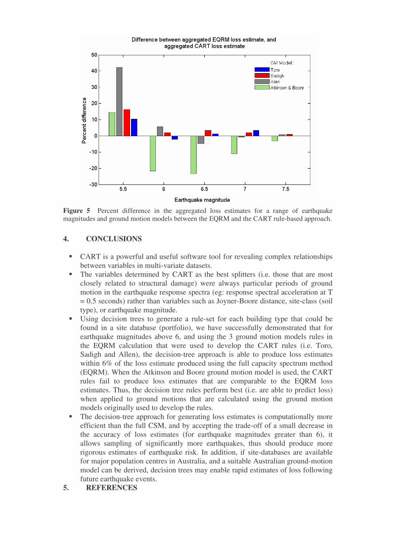
Figure 5 Percent difference in the aggregated loss estimates for a range of earthquake magnitudes and ground motion models between the EQRM and the CART rule-based approach.

4. CONCLUSIONS

� CART is a powerful and useful software tool for revealing complex relationships

between variables in multi-variate datasets. � The variables determined by CART as the best splitters (i.e. those that are most

closely related to structural damage) were always particular periods of ground motion in the earthquake response spectra (eg: response spectral acceleration at T = 0.5 seconds) rather than variables such as Joyner-Boore distance, site-class (soil type), or earthquake magnitude.

� Using decision trees to generate a rule-set for each building type that could be found in a site database (portfolio), we have successfully demonstrated that for earthquake magnitudes above 6, and using the 3 ground motion models rules in the EQRM calculation that were used to develop the CART rules (i.e. Toro, Sadigh and Allen), the decision-tree approach is able to produce loss estimates within 6% of the loss estimate produced using the full capacity spectrum method (EQRM). When the Atkinson and Boore ground motion model is used, the CART rules fail to produce loss estimates that are comparable to the EQRM loss estimates. Thus, the decision tree rules perform best (i.e. are able to predict loss) when applied to ground motions that are calculated using the ground motion models originally used to develop the rules.

� The decision-tree approach for generating loss estimates is computationally more efficient than the full CSM, and by accepting the trade-off of a small decrease in the accuracy of loss estimates (for earthquake magnitudes greater than 6), it allows sampling of significantly more earthquakes, thus should produce more rigorous estimates of earthquake risk. In addition, if site-databases are available for major population centres in Australia, and a suitable Australian ground-motion model can be derived, decision trees may enable rapid estimates of loss following future earthquake events.

5. REFERENCES

Atkinson, G.M. and Boore, D.M., (1997) Some comparisons between recent ground-

motion relations. Seismological Research Letters, Vol. 66(1), pp24-40. Freeman, S.A., (2004) Review of the development of the capacity spectrum method.

ISET Journal of Earthquake Technology, Paper No. 438, Vol. 41, No. 1, pp1-13. Kircher, C.A., Nassar, A.A., Kustu, O. and Holmes, W.T., (1997) Development of

Building Damage Functions for Earthquake Loss Estimation. Earthquake Spectra, Vol 13(4), pp663-682

Lewis, R.J., (2000) An Introduction to Classification and Regression Tree (CART) Analysis.

Patchett, A.M., Robinson, D., Dhu, T. and Sanabria, A., (2005) Investigating Earthquake Risk Models and Uncertainty in Probabilistic Seismic Risk Analyses. Geoscience Australia, Record 2005/02.

Robinson, D., Fulford, G., and Dhu, T., (2005) EQRM: Geoscience Australia’s Earthquake Risk Model. Technical Manual Version 3.0. Geoscience Australia Record 2005/01.

Sadigh, K., Chang, J.A., Egan, J.A., Makdisi, F. and Youngs, R.R., (1997) Attenuation relationships for shallow crustal earthquakes based on California strong motion data. Seismological Research Letters, Vol. 68(1), pp180-189.

Toro, G.R., Abrahamson, N.A., and Schneider, J.F., (1997) Model of strong ground motions from earthquakes in Central and Eastern North America: Best estimates and certainties. Seismological Research Letters, Vol 68(1), 41-57.