using data in excel - ohio early...

Ohio Department of Developmental Disabilities of 51 Using Data in Excel (2016 Data and Monitoring Road Show) Revised 9/22/16

Using Data in Excel Note: This document was created as a resource for the 2016 Data and Monitoring Road Show trainings The following instructions are intended to provide some commonly used Excel functions, formulas, and procedures, both in general, and specific to the Program Referrals Extract Report and EI Services Report. All of the instructions refer to how to perform tasks in Microsoft Excel 2013, so some steps may differ if using a different version of the software. Additionally, Excel can be used for countless other purposes, and there are multiple approaches for accomplishing most tasks using Excel.

Program Referral Extract

Formatting Copy and paste all into new worksheet In order to retain original data, it’s helpful to select the entire dataset and copy into a new worksheet prior to altering the dataset in any way.

Press “Ctrl” and “A” simultaneously to select all data in the sheet

Press “Ctrl” and “C” to copy all of the data or Right Click and choose “Copy”

In a new sheet, press “Ctrl” and “V” simultaneously to paste the previously copied data Rename worksheet Naming each worksheet with a short description of what data are included helps quickly navigate needed data

Right click on the worksheet and Click “Rename” or Double click on the worksheet title

Type desired name


Change font

Select desired cell/area

Navigate to the “HOME” tab toward the left of the Excel ribbon

Select desired font from the drop down in the Font are

Remove “Wrap Text” “Wrap Text” is a formatting function that adjusts the row height in order to ensure all text within the cell is visible. Depending on the desired layout of the worksheet, it can be helpful to turn the wrap text feature on or off.

Select desired cells or area

Unselect the “Wrap Text” option in the Alignment box in the “HOME” tab


Delete extra row

Click in the pane to the left of the row(s) to be deleted (labeled 1, 2, 3…)

Right click in the selected area

Select “Delete” from the drop down

Make header row bold

Click in the pane to the left of the row (labeled 1, 2, 3…)


Navigate to the “HOME” tab

Click on the “B”

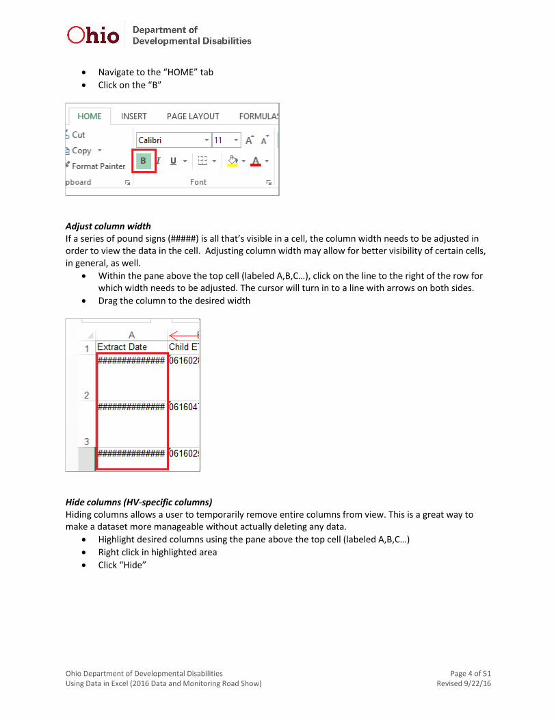
Adjust column width If a series of pound signs (#####) is all that’s visible in a cell, the column width needs to be adjusted in order to view the data in the cell. Adjusting column width may allow for better visibility of certain cells, in general, as well.

Within the pane above the top cell (labeled A,B,C…), click on the line to the right of the row for which width needs to be adjusted. The cursor will turn in to a line with arrows on both sides.

Drag the column to the desired width

Hide columns (HV-specific columns) Hiding columns allows a user to temporarily remove entire columns from view. This is a great way to make a dataset more manageable without actually deleting any data.

Highlight desired columns using the pane above the top cell (labeled A,B,C…)

Right click in highlighted area

Click “Hide”


Using filters Filters can be helpful to temporarily select only certain rows of data, based on desired criteria.

Select the top (header) row within the data set by clicking in the pane to the left of the row

Navigate to the “DATA” tab of the Excel ribbon in the Sort & Filter section and select “Filter” to turn filters on

Click the downward facing triangle in any cell to select information to filter (examples are included subsequently

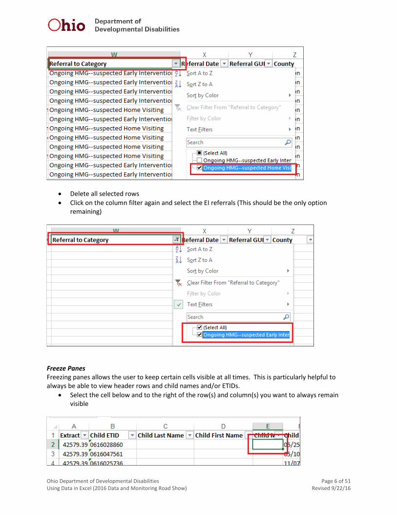
Remove extra information Removing extra data from your working file makes navigating the dataset simpler and more straightforward. For this report, removing the Home Visiting information can make the data easier to work with if you only need the fields related to EI.

Make sure filters are turned on in the top row

Navigate to the “Referral to Category” column

Click on the filter box within in the column header

Select all home visiting referrals by making sure only the “Ongoing HMG—suspected Home Visiting” box is checked


Delete all selected rows

Click on the column filter again and select the EI referrals (This should be the only option remaining)

Freeze Panes Freezing panes allows the user to keep certain cells visible at all times. This is particularly helpful to always be able to view header rows and child names and/or ETIDs.

Select the cell below and to the right of the row(s) and column(s) you want to always remain visible


Navigate to the “VIEW” tab on the Excel ribbon and select “Freeze Panes”

Click “Freeze Panes” from the drop down

Cell formatting There are many different options for structuring cells that can distinguish them, make them easier to read, or ensure they are in the needed format. The method described subsequently can also be used to perform many of the tasks described previously.

Highlight cell(s) for which you desire a change in format

Right click within the highlighted area

Choose “Format Cells”


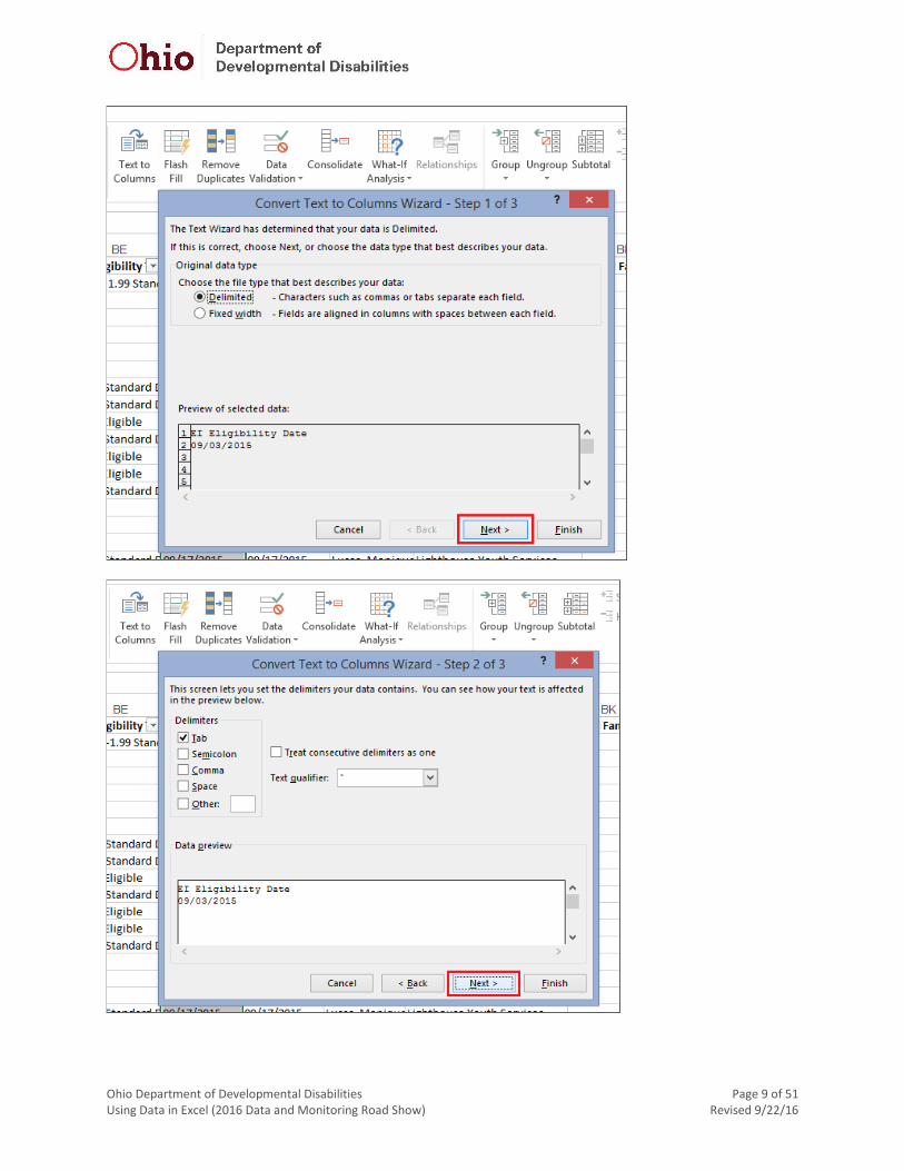
Convert from text to other formats Sometimes data are configured in such a way that the cell formatting changes won’t initially “take.” Though it opens in Excel, the Program Referrals Extract is an example of this, as it is actually formatted as a text file. Thus, a few extra steps are needed in order to convert data to a different format then text:

Highlight the cells needing formatting changes

Navigate to the “DATA” tab on the Excel Ribbon

Click on “Text to Columns” in the Data Tools area

Utilize the default options and click “Next” at Step 1 and Step 2 and “Finish” at Step 3

Once the text to column conversion is complete, follow the steps above to format cells as desired


Calculations Formulas Formulas in Excel are a very useful way to calculate values. Several pre-defined formulas, called functions, are available in Excel. In addition to the readily available functions, many other formulas can be used to make calculations. Formulas include the following components:

Equals sign (=): Each formula begins with an equals sign and is followed by one or more of the subsequent components

Cell references: Many times, formulas include references to particular cell, defined by the column letter and row number (e.g., A1)

Operators: These are the components that specify the type of calculation that should be performed

Constants: Some formulas contain text or numbers in addition to or instead of cell references


Third Birthday The ‘EDATE’ formula calculates a date that is the specified number of months from the date in the referenced cell. Because children can be served in Early Intervention until age three, calculating the third birthday is useful in a lot of circumstances for cleaning data or making calculations.

Right click the “Child Due Date” column in the pane above the top cell (labeled A,B,C…)

Select “Insert” to add a new column to the right of the “Child Birth Date” column

Name the column “Third Birthdate”

Click in the top cell and type the formula “=EDATE(F2,36)” and press enter. In this example, “F2” was referenced (Column F, Row 2), as that was the cell where the child’s birth date was located, so this formula may need to be adjusted to reference the proper cell. “36” was used to calculate the date that is 36 months from the child’s birthday, or the child’s third birthday, so that number can also be adjusted as needed to make different calculations.


Autofill column with third birth date for each child When the same information (number, formula, etc.) needs to be included in every cell within a column, the autofill function is very helpful. In this case, the third birthday needs to be calculated for every child, so the formula can be copied into each cell within the column to the end of the data file. This function works best when no filters are on.

Navigate to the bottom right corner of the cell that contains the formula you intend to copy. You will see a cross display in place of your pointer so you know that you are in the right location. Double click in this location, and the formula will be copied into each cell in the column.

Copy and Paste Special The ‘Paste Special’ function is useful for selecting a group of information and pasting it all into a different format.

Once the formulas have been copied, highlight the “Third Birthday” column

Press “Ctrl” and “C” simultaneously to copy the data

Right click within the column, and select the second paste option with the “123” at the bottom of the clipboard image

If not automatically done, format the column as dates


Create New Variables Create variable to label referral month Adding additional variables, or creating new columns to label a group of data, can be helpful for filtering or sorting data, as well as creating PivotTables (described later in this document).

Insert a column to the right of the “Referral Date” column

Label the column “Referral month”

Select the “Referral month column”

Right click within the column and select “Format Cells”

In the pop-up box, select “Text” from the “Number” tab, then click “OK”


Click the filter of the “Referral Date” column

Select desired month


Type month name and year in the first cell of the “Referral Month” column

Click on the cell to select it and move your mouse to the bottom right corner until the cursor appears as a plus sign

Click the bottom right corner of the cell and drag your mouse downward until you get to the end of the file

Repeat until all desired months have been labeled in the “Referral Month” Column

Create variable to indicate whether the child was determined eligible Creating a ‘Yes’ or ‘No’ variable can help make it more straightforward to select or view only certain desired data. In this case, the new variable simply states whether the child has an eligibility determination entered in the data system.

Insert a column to the right of the “EI Eligibility Date” column and title it “Eligibility?”

Click on the filter for the “EI Eligibility Date” column o Note: The eligibility date may be earlier than the referral date (e.g., for a child who was

previously served in EI, exited, and then re-referred)

Unselect “(Blanks)”

Click on the filter in the “EI Eligibility Type” column

Unselect “Not Eligible”


Type “Yes” into the first row of the “Eligibility?” column

Click on the cell to select it and move your mouse to the bottom right corner until the cursor appears as a plus sign


Select the top row

Navigate to “Filter” in the “Sort & Filter” section of “DATA” tab of the Excel ribbon, and turn the filter off and back on to remove all filters

Select the “Eligibility?” column

Navigate to the “HOME” tab in the Excel ribbon and click on “Find & Select” within the “Editing” section


A “Find and Replace” pop up box will appear

Keep the “Find what” box blank and type “No” into the “Replace with” box

Click “Replace All” or Press “Enter”


Create a variable to indicate whether a determination about Need for Services was made for the child This is another ‘Yes’ or ‘No’ variable that indicates whether the child had a Need for Services established.

Insert a column to the right of the “EI Initial NFS date in referral period” column and title it “NFS?”

Click on the filter for the “EI Initial NFS date in referral period” column

Unselect “(Blanks)”

Type “Yes” into the first row of the “NFS?” column

Click on the row to select it and move your mouse to the bottom right corner until the cursor appears as a plus sign


o NOTE: If “No NFS” is selected in a child record, the date is still included in this column. There is no way to distinguish which children had “No NFS” entered, but it’s very rare that that happens, as most children without a NFS also weren’t established eligible, and therefore don’t have anything entered on the NFS page.

Select the top row



Select the “NFS?” column





Create a variable to indicate whether the child had an IFSP This is yet another ‘Yes’ or ‘No’ variable that specifies whether a child was served in EI (had at least one IFSP).

Insert a column to the right of the “Initial Ifsp Date” column and title it “IFSP?”

Click on the filter for the “Initial Ifsp Date” column

Scroll down and unselect “(Blanks)”


Type “Yes” into the first row of the “IFSP?” column

Click on the row to select it and move your mouse to the bottom right corner until the cursor appears as a plus sign


Select the top row


Select the “IFSP?” column



Pivot Tables Create a PivotTable PivotTables are an extremely useful tool in Excel that can be used relatively easily to analyze and organize, and ultimately to share, a broad array of data.

Navigate to the “Insert” tab

Click on “PivotTable”

By default, the PivotTable will include all columns and cells of the worksheet and will populate in a new worksheet

o Note: If there are any completely blank columns in the middle of a dataset, the table will include all columns to the left of the blank column by default

Click “OK” to create a blank PivotTable table in a new sheet

A new worksheet will appear to the left of worksheet from which the data were selected

A blank PivotTable will appear on the left side of the new worksheet, and the available PivotTable fields along with options for columns, rows, filters, and values will appear on the right


Referrals by Month To determine number of referrals that occurred each month, a PivotTable that includes the ‘Referral Month’ variable is extremely useful.

Scroll down in the PivotTable fields and move the cursor to the “Referral Month” field

Drag the “Referral Month” field down to the “ROWS” box

Also drag the “Referral Month” to the “VALUES” box

Your PivotTable of referrals by month will be displayed at the left of the worksheet


Referral Sources A PivotTable that includes the ‘Referral Source Type’ will indicate the number of referrals within a particular time period that came from each different referral source.

Select the entire Referral Month PivotTable

Paste table below the original

Drag and drop the “Referral Source Type” field into the “ROWS” and “VALUES” boxes

Remove the “Referral Month” field from both boxes


Referral Outcome by Referral Source Type – Children Served A PivotTable that includes the ‘Referral Source Type’ and ‘IFSP?’ variables will provide information about the number (and/or percentage) of referrals from each referral source that ultimately resulted in the child being served in EI.

Select the entire Referral Source Type PivotTable

Paste table below the original

Drag the “IFSP?” field into the “COLUMNS” box

To show values of zero, click anywhere within the table

Navigate to the “ANALYZE” tab

Click on “Options” and select “Options” from the drop down


In the PivotTable options pop-up, within the “Layout & Formula” tab, enter “0” in the “For empty cells show:” box

Click “OK”


To calculate the percentage of referrals for each referral source that resulted in the child being served, click in the cell that corresponds to the top row and the column directly to the right of the table

Type the following formula: “=C48/D48” (Adjust as necessary so the formula references the proper cells)

Click the bottom right corner of the cell and drag your mouse downward until you get to the end of the table

Use the cell format options to format the data as you’d like


EI Services Service Compliance Calculating Service Due Date Calculating the date by which a service must occur in order to be considered timely is important for monitoring compliance with the federally required Timely Receipt of Services indicator. This can be achieved using a simple formula.

Select the “Start Date” column and insert a new column

Label the new column “Service Due Date”

In the top cell of the “Service Due Date” column, type the following formula: “=T2+30” (adjust formula as necessary to reference the “IFSP Added Date” column) to calculate the date that is 30 days from the date the service was added to the IFSP

Double click the bottom right corner of the cell to autofill the formula to the end of the column

Once the formulas have been copied, highlight the “Service Due Date” column

Press “Ctrl” and “C” simultaneously to copy the data

Right click within the column, and select the second paste option with the “123” at the bottom of the clipboard image to past the values into the cells


Selecting service due dates in the desired timeframe Typically, when determining whether TRS compliance requirements have been met, a specific time range of TRS due dates is of particular interest. Narrowing down the due dates to the desired range is a two-step process. First, it needs to be determined whether the IFSP in that row is the one to which the service was added and, if not, that row needs to be removed. Second, services outside of the desired time range need to be removed.

Insert a column to the right of the “IFSP Added Date” column

To determine whether the IFSP date referenced in the row is the date the service-outcome combination was added to the IFSP, use the following formula: “=IF(T2=L2,“Yes”,”No”)”

Autofill the formula to the end of the column

Copy the entire column and paste as values

Make sure filters are turned on and select “No” from the filter in the newly created column – these are the rows where the “IFSP Date” is not equal to the “IFSP Added Date”

Remove all selected rows

Turn filters off and back on

Next, use the filter in the “Service Due Date” column to select all dates NOT in the desired time frame

Delete all selected rows

Turn filter off and back on, and only desired TRS Due dates will remain


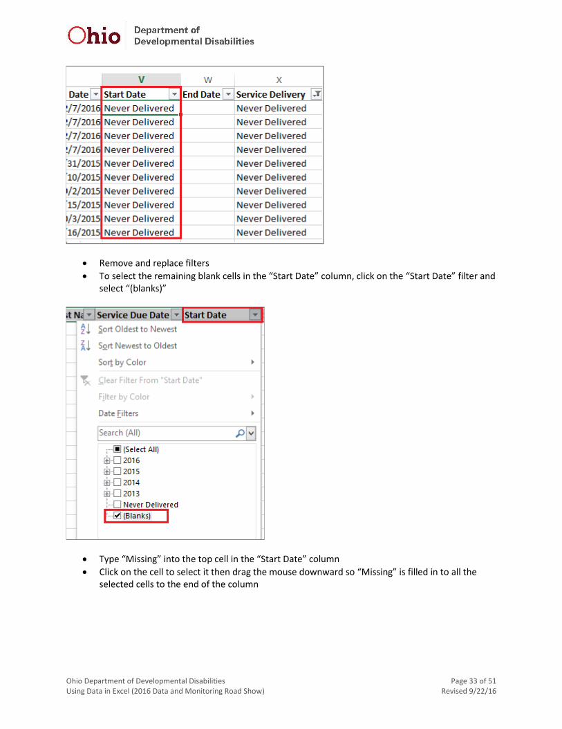
Calculating number of days it took for service delivery to begin Another relatively simple formula can be used to calculate the number of days after a service was added to an IFSP that the initial service delivery occurred, while accounting for any missing service start dates. A date can be missing because the “Never Delivered” option and a non-compliance reason have been selected or because a start date had not been entered into the system at the time data were extracted.

The blank cells in the “Start Date” column first need to be labeled as “Never Delivered” or “Missing”

Click on the “Start Date” filter

Select only “(blanks)”

Click on the “Service Delivery” filter

Select “Never Delivered”

Type “Never Delivered” into the top cell in the “Start Date” column

Click on the cell to select it then drag the mouse downward so “Never Delivered” is filled in to the selected cells to the end of the column


Remove and replace filters

To select the remaining blank cells in the “Start Date” column, click on the “Start Date” filter and select “(blanks)”

Type “Missing” into the top cell in the “Start Date” column

Click on the cell to select it then drag the mouse downward so “Missing” is filled in to all the selected cells to the end of the column


Select the “End Date” column and insert a new column

Label the new column “Start Minus IFSP”

Click in the top cell of the “Start Minus IFSP Column” and type the following formula: “=IF(V2="Missing","Missing",IF(V2="Never Delivered","Never Delivered",V2-T2))”

o This formula looks at the cell and if the “Start Date” column is listed as “Missing” or “Never Delivered” then the “Start Minus IFSP” column is labeled the same; otherwise, this formula calculates the number of days from the IFSP to the start of the service

o T2 and V2 specifically refer to the “IFSP Added Date” and “Start Date” columns, so if these columns are in different locations within your file, adjust accordingly

Double click in the bottom right corner of the cell to autofill the formula into each cell in the column

Copy the content of the entire column and “Paste special” to paste only the values in each cell


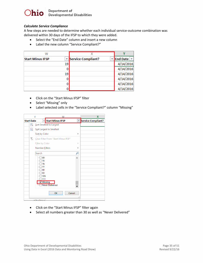
Calculate Service Compliance A few steps are needed to determine whether each individual service-outcome combination was delivered within 30 days of the IFSP to which they were added.

Select the “End Date” column and insert a new column

Label the new column “Service Compliant?”

Click on the “Start Minus IFSP” filter

Select “Missing” only

Label selected cells in the “Service Compliant?” column “Missing”

Click on the “Start Minus IFSP” filter again

Select all numbers greater than 30 as well as “Never Delivered”


Click on the “Non-Compliance Reason” filter

Select “Parent/Child reason,” “Couldn’t locate/reach parent,” and “Emergency related closure,” as applicable

o Note: These options will only show up if they exist in a cell within the column for which the filter is being selected


Label each visible cell in the “Service Compliant?” column as “With NCR”

Click on the “Non-Compliance Reason” filter again

This time select “HMG staff error” and “HMG system reason,” as applicable

Label each visible cell in the “Service Complaint?” column as “No”


Click on the “Service Compliant”

Select “(Blanks)”

Click on the “Start Minus IFSP” filter and check to ensure the only values are numbers 1 through 30

Label each visible cell in the “Service Compliant?” column as “Yes”


EI Services on IFSPs Remove Duplicates If you want to determine a total count of something that is repeated in multiple rows within your dataset, the “Remove Duplicates” feature is helpful. For example, if you want to know how many children had particular services added to IFSPs that occurred within the specified timeframe, you can remove duplicates by ETID and Service Type, which will leave only the first row that contains the ETID and Service Type, and the rest will be deleted from the file (Note: The ETID and Service Type could be duplicated because a child has a service that is needed to meet multiple outcomes on the same IFSP or on two different IFSPs within the specified timeframe.)

Copy and paste all data into a new worksheet

Navigate to the “DATA” tab and click on “Remove Duplicates”


Click “Unselect All”

Check “ETID” and “Service Type” then click “OK”

NOTE: Always be cognizant of the specific data that are being de-duplicated and what that means. For instance, in this example, some data had already been removed from the original data set and only services added within the specified timeframe were left.

Create PivotTable of Services To see the number of children who had each Service Type added to an IFSP within the specified timeframe, a PivotTable using the “Service Type” field can be created.

Navigate to the “Insert” tab of the worksheet that includes the desired data

Click on “PivotTable”

A new worksheet will be created, where the PivotTable can be designed

Drag the “Service Type” field down to the “ROWS” box and again to the “VALUES” box


Your PivotTable will generate at the left of the open worksheet

Finally, if there’s something you want to do in Excel, but don’t know how… USE THE INTERNET! Though the Data and Monitoring Team are always happy to answer questions, almost anything you want to learn or know how to do in Excel can be found quickly and easily by simply typing in whatever it is you’d like to know in your search engine of choice.

using data in excel - ohio early...

Documents