using computational intelligence for the safety...

Using Computational Intelligencefor the Safety Assessment of Oiland Gas Pipelines: A Survey

Abduljalil Mohamed, Mohamed Salah Hamdi and Sofiène Tahar

Abstract The applicability of intelligent techniques for the safety assessment of oiland gas pipelines is investigated in this study. Crude oil and natural gas are usuallytransmitted through metallic pipelines. Working under unforgiving environments,these pipelines may extend to hundreds of kilometers, which make them verysusceptible to physical damage such as dents, cracks, corrosion, etc. These defects,if not managed properly, can lead to catastrophic consequences in terms of bothfinancial losses and human life. Thus, effective and efficient systems for pipelinesafety assessment that are capable of detecting defects, estimating defects sizes, andclassifying defects are urgently needed. Such systems often require collectingdiagnostic data that are gathered using different monitoring tools such as ultra-sound, magnetic flux leakage, and Closed Circuit Television (CCTV) surveys. Thevolume of the data collected by these tools is staggering. Relying on traditionalpipeline safety assessment techniques to analyze such huge data is neither efficientnor effective. Intelligent techniques such as data mining techniques, neural net-works, and hybrid neuro-fuzzy systems are promising alternatives. In this paper,different intelligent techniques proposed in the literature are examined; and theirmerits and shortcomings are highlighted.

Keywords Oil and gas pipelines ⋅ Safety assessment ⋅ Big data ⋅ Computa-tional intelligence ⋅ Data mining ⋅ Artificial neural networks ⋅ Hybridneuro-fuzzy systems ⋅ Artificial intelligence ⋅ Defect sizing ⋅ Magnetic fluxleakage

A. Mohamed (✉) ⋅ M.S. HamdiDepartment of Information Systems, Ahmed Bin Mohamed Military College,P. O. Box 22713, Doha, Qatare-mail: [email protected]

M.S. Hamdie-mail: [email protected]

S. TaharDepartment of Electrical and Computer Engineering, Concordia University,1515 St. Catherine W, Montreal, Canadae-mail: [email protected]

© Springer International Publishing AG 2017W. Pedrycz and S.-M. Chen (eds.), Data Science and Big Data:An Environment of Computational Intelligence, Studies in Big Data 24,DOI 10.1007/978-3-319-53474-9_9

189

1 Introduction

Oil and gas are the leading sources of energy the world relies on today; andpipelines are viewed as one of the most cost efficient ways to move that energy anddeliver it to consumers. The latest data, in 2015, gives a total of more than 3.5million km of pipeline in 124 countries of the world. Many other thousands ofkilometers of pipelines are planned and under construction. Pump stations, alongthe pipeline, move oil and gas through the pipelines. Because the pipeline walls areunder constant pressure, tiny cracks may arise in the steel. Under the continuousload, they can then grow into critical cracks or even leaks. Pipelines conveyingflammable or explosive material, such as natural gas or oil, pose special safetyconcerns; and various accidents have been reported [1]. Damage to the pipelinemay cause the occurrence of large and enormous human and economic losses.Moreover, damaged pipelines obviously represent an environmental hazard.Therefore, pipeline operators must identify and remove pipeline failures caused bycorrosion and other types of defects as early as possible.

Today, inspection tools, called “Pipeline Inspection Gauges” or “Smart Pigs”,employ complex measuring techniques such as ultrasound and magnetic fluxleakage. They are used for the inspection of such pipelines, and have become majorcomponents to pipeline safety and accident prevention. These smart pigs areequipped with hundreds of highly tuned sensors that produce data that can be usedto locate and determine the thickness of cracks, fissures, erosion and other problemsthat may affect the integrity of the pipeline. In each inspection passage, hugeamounts of data (several hundred gigabytes) are collected. A team of experts willlook at these data and assess the health of the pipeline segments.

Because of the size and complexity of pipeline systems and the huge amounts ofdata collected, human inspection alone is neither feasible nor reliable. Automatingthe inspection process and the evaluation and interpretation of the collected datahave been an important goal for the pipeline industry for a number of years.Significant progress has been made in that regard, and we currently have a numberof techniques available that can make the highly challenging and computationally-intensive task of automating pipeline inspection possible. These techniques rangefrom analytical modeling, to numerical computations, to methods employing arti-ficial intelligence techniques such as artificial neural networks. This paper presentsa survey of the state-of-the-art in methods used to assess the safety of the oil and gaspipelines, with emphasis on intelligent techniques. The paper explains the princi-ples behind each method, highlights the settings where each method is mosteffective, and shows how several methods can be combined to achieve higheraccuracy.

The rest of the paper is organized as follows. In Sect. 2, we review the fivestages of the pipeline reliability assessment process. The theoretical principalsbehind the intelligent techniques surveyed in this study are discussed in Sect. 3. In

190 A. Mohamed et al.

Sect. 4, the pipeline safety assessment approaches using the intelligent techniquesreported in Sect. 3 are presented and analyzed. We conclude with final remarks inSect. 5.

2 Safety Assessment in Oil and Gas Pipelines

The pipeline reliability assessment process is basically composed of five stages,namely data processing, defect detection, determination of defect size, assessmentof defect severity, and repair management. Once a defect is detected, the defectassessment unit proceeds by determining the size (the defect’s depth and length) ofthe defect. This is really an important step as the severity of the defect is based onits physical characteristics. Based on the severity level of the detected defect, anappropriate action is taken by the repair management. These five stages of thepipeline assessment process are summarized in the following subsections.

2.1 Big Data Processing

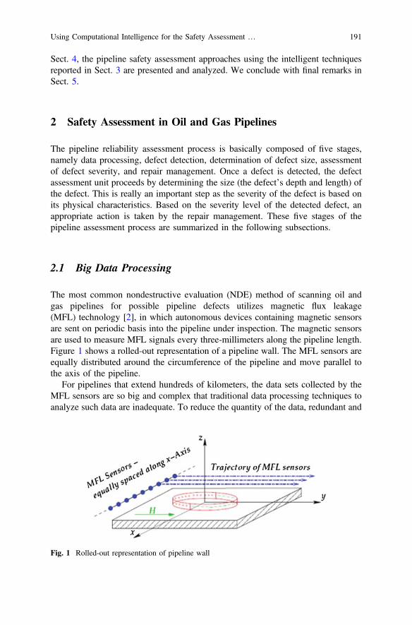
The most common nondestructive evaluation (NDE) method of scanning oil andgas pipelines for possible pipeline defects utilizes magnetic flux leakage(MFL) technology [2], in which autonomous devices containing magnetic sensorsare sent on periodic basis into the pipeline under inspection. The magnetic sensorsare used to measure MFL signals every three-millimeters along the pipeline length.Figure 1 shows a rolled-out representation of a pipeline wall. The MFL sensors areequally distributed around the circumference of the pipeline and move parallel tothe axis of the pipeline.

For pipelines that extend hundreds of kilometers, the data sets collected by theMFL sensors are so big and complex that traditional data processing techniques toanalyze such data are inadequate. To reduce the quantity of the data, redundant and

Fig. 1 Rolled-out representation of pipeline wall

Using Computational Intelligence for the Safety Assessment … 191

irrelevant data are removed using feature extraction and selection techniques. Themost relevant features are selected, and then used to determine the depth and lengthof the detected defect.

2.2 Defect Detection

In this stage, the diagnostic data are examined for the existence of possible defectsin the pipeline. To detect and identify the location of potential defects, wavelettechniques are widely used [3]. They are very powerful mathematical methods [4–6]. They were reported in many applications such as data compression [7], dataanalysis and classification [8], and de-noising [9–11].

2.3 Determination of Defect Size

To determine the severity level of the detected defect, the defect’s depth and lengthare calculated. However, the relationship between the given MFL signals andparticular defect type and shape is not well-known. Hence, it is very difficult toderive an analytical model to describe this relationship. To deal with this problem,researchers resort to intelligent techniques to estimate the required parameters. Oneof these intelligent tools is the Adaptive Neuro-Fuzzy Inference System (ANFIS).

2.4 Assessment of Defect Severity

Based on the defect parameters (i.e., depth and length) obtained in the previousstage, an industry standard known as ASME B31G is often used to assess theseverity level of the defect [12]. It specifies the pipeline stress under operatingpressure and what defect parameters that may fail the hydro pressure test [13].

2.5 Repair Management

In order to determine an appropriate maintenance action, the repair managementclassifies the severity level of pipeline defects into three basic categories, namely:severe, moderate, and acceptable. Severe defects are given the highest priority andan immediate action is often required. The other two severity levels are not deemedcritical, thus, a repair action can be scheduled for moderate and acceptable defects.


3 Computational Intelligence

As mentioned in the previous section, MFL signals are widely used to determine thedepth and length of potential defects. From recorded data, it has been observed thatthe magnitude of MFL signals varies from one defect depth and length to another.In the absence of analytical models that can describe the relationship between theamplitude of MFL signals and their corresponding defect dimensions, computa-tional intelligence provides an alternative approach. Given sufficient MFL data,there are different computational techniques such as data mining techniques, arti-ficial neural networks, and hybrid neuro-fuzzy systems that can be utilized to learnsuch relationships. In the following, the theoretical principals behind each of thesetechniques are summarized.

3.1 Data Mining

The k-nearest neighbor (k-NN) and support vector machines (SVM) are widelyused in data mining to solve classification problems. Within the context of thesafety assessment in oil and gas pipelines, these two techniques can be employed toassign detected defects to a certain severity level.

3.1.1 K-Nearest Neighbor (KNN)

The KKN is a non-parametric learning algorithm as it does not make anyassumptions on the underlying data distribution. This may come in handy sincemany real world problems do not follow such assumptions. The KNN learningalgorithm is also referred to as a lazy algorithm because it does not use the trainingdata points to do any generalization. Thus, there is no training stage in the learningprocess, but rather KNN makes its decision based on the entire training data set.The learning algorithm assumes that all instances correspond to points in then-dimensional space. The nearest neighbors of an instance are identified using thestandard Euclidean distance. Let us assume that a given defect x is characterized bya feature vector:

⟨a1ðxÞ, a2ðxÞ, . . . , anðxÞ⟩, ð1Þ

where ar xð Þ denotes the value of the rth attribute of instance x. Thus, the distanced between two instances xi and xj is calculated as follows:

d xi, xj� �

=

ffiffiffiffiffiffiffiffiffiffiffiffiffiffiffiffiffiffiffiffiffiffiffiffiffiffiffiffiffiffiffiffiffiffiffiffiffiffiffiffiffi∑n

r=1ar xið Þ− ar xj

� �� 2s, ð2Þ


For the safety assessment in oil and gas pipeline application, the target functionis discrete. That is, it assigns the feature vector of the detected defect to one of thethree severity levels severe, moderate, or acceptable. If we suppose k=1, then the1-nearest neighbor assigns the feature vector to the severity level where the traininginstance of that severity level is nearest to the feature vector. For larger values of k,the algorithm assigns the most common severity level among the k nearest trainingexamples. e only assumption made is that the data is in a feature space.

3.1.2 Support Vector Machine (SVM)

The SVM is a discriminant classifier defined by a separating hyperplane. Givenlabeled training data, the SVM algorithm outputs an optimal hyperplane that cancategorize new examples. Support vector machines are originally designed forbinary classification problems. For a linearly separable set of 2D-points, there willbe multiple straight lines that may offer a solution to the problem. However, a line isconsidered bad if it passes too close to the points because it will be susceptible tonoise. The task of the SVM algorithm is to find the hyperplane that gives the largestminimum distance (i.e., margin) to the training examples.

To solve multi-class classification problems, the SVM should be extended. Thetraining algorithms of SVMs look for the optimal separating hyperplane which hasa maximized margin between the hyperplane and the data, which in turn, minimizesthe classification error. The separating hyperplane is represented by a small numberof training data, called support vectors (SVs). However, the real data cannot beseparated linearly, thus the data are mapped into a higher dimensional space.Practically, a kernel function is utilized to calculate the inner product of thetransformed data. The efficiency of the SVM depends mainly on the kernel.

Formally, the hyperplane is defined as follows:

f ðxÞ= β0 + βTx, ð3Þ

where β is known as the weight vector and β0 as the bias. The optimal hyperplanecan be represented in an infinite number of different ways by scaling of β and β0.The hyperplane chosen is:

β0 + βTx�� =1, ð4Þ

where x symbolizes the training examples closest to the hyperplane, which arecalled support vectors. The distance between a point x and a hyperplane ( β,β0) canbe calculated as:

distance=β0 + βTx��

βk k , ð5Þ

For the canonical hyperplane, the numerator is equal to one, thus,


distance=β0 + βTx��

βk k =1βk k , ð6Þ

The margin (M) is twice the distance to the closest examples:

M =2βk k , ð7Þ

Now, maximizing M is equivalent to the problem of minimizing a function L βð Þsubject to some constrains as follows:

minβ, β0

L βð Þ= 12βj j2, ð8Þ

subject to:

yi = βTxi + β0� �

≥ 1∀i, ð9Þ

where yi represents each of the labels of the training examples.

3.2 Artificial Neural Networks

Artificial neural networks (ANN) are suitable for the safety assessment in oil andgas pipelines as they are capable of solving ill-defined problems. Essentially theyattempt to simulate the neural structure of the human brain and its functionality.

The multi-layer perceptron (MLP) with the back propagation learning algorithmis considered the most common neural network and being widely used in a largenumber of applications. A typical MLP neural network of one hidden layer isdepicted in Fig. 2. There are d inputs (example, d dimensions of input pattern X), hhidden nodes, and c outputs nodes.

The output of the jth hidden node is zj = fjðajÞ, where aj = ∑di=0 wjixi, and fjð.Þ is

an activation function associated with hidden node j. wji is the connection weightfrom the input node i to j, and wj0 denotes the bias for the hidden node j. For aninput node k, its output is yk = fkðakÞ, where ak = ∑h

j=0 wkjzj, and fkð.Þ is the acti-vation function associated with output node k. wkj is the connection weight fromhidden node j to output node k. wk0 denotes the bias for output node k. The acti-vation function is often chosen as the unipolar sigmoidal function:

f ðaÞ= 11+ expð− γaÞ , ð10Þ


In MLP, the back propagation learning algorithm is used to update weights so asto minimize the following squared error function:

JðwÞ= 12∑c

k=1ðek − ykðXÞÞ2, ð11Þ

3.3 Hybrid Neuro-Fuzzy Systems

The focus of intelligent hybrid systems in this study will be on the combination ofneural networks and fuzzy inference systems. One of these systems is the adaptiveneuro-fuzzy inference system (ANFIS), which will be used as an illustrativeexample of such hybrid systems. ANFIS, as introduced by Jang [14], utilizes fuzzyIF-THEN rules, where the membership function parameters can be learned fromtraining data, instead of being obtained from an expert [15–23]. Whether thedomain knowledge is available or not, the adaptive property of some of its nodesallows the network to generate the fuzzy rules that approximate a desired set ofinput-output pairs. In the following, we briefly introduce the ANFIS architecture asproposed in [14]. The structure of the ANFIS model is basically a feedforwardmulti-layer network. The nodes in each layer are characterized by their specificfunction, and their outputs serve as inputs to the succeeding nodes. Only theparameters of the adaptive nodes (i.e., square nodes in Fig. 3) are adjustable duringthe training session. Parameters of the other nodes (i.e., circle nodes in Fig. 3) arefixed.

Fig. 2 A multi-layer perceptron neural network


Suppose there are two inputs x, y, and one output f. Let us also assume that thefuzzy rule in the fuzzy inference system is depicted by one degree of Sugeno’sfunction [14].

Rule 1: if x is A1 and y is B1 then f = p1x+ q1y+ r1Rule 2: if x is A2 and y is B2 then f = p2x+ q2y+ r2

where pi, qi, ri are adaptable parameters.The node functions in each layer are described in the sequel.

Layer 1: Each node in this layer is an adaptive node and is given as follows:

o1i = μAiðxÞ, i=1, 2

o1i = μBi− 2ðyÞ, i=3, 4

where x and y are inputs to the layer nodes, and Ai and Bi− 2 are linguisticvariables. The maximum and minimum of the bell-shaped membershipfunction are 1 and 0, respectively. The membership function has thefollowing form:

μAiðxÞ=1

1+ x− ciai

� �2� bi , ð12Þ

where the set ai, bi, cif g represents the premise parameters of themembership function. The bell-shaped function changes according to thechange of values in these parameters.

Layer 2: Each node in this layer is a fixed node. Its output is the product of thetwo input signals as follows:

Fig. 3 The architecture of ANFIS


o2i =wi = μAiðxÞμBiðyÞ, i=1, 2, ð13Þ

where wi refers to the firing strength of a rule.Layer 3: Each node in this layer is a fixed node. Its function is to normalize the

firing strength as follows:

o3i =w′′

i =wi

w1 +w2, i=1, 2 ð14Þ

Layer 4: Each node in this layer is adaptive and adjusted as follows:

o4i =w′′

i fi =w′′

i pix+ qiy+ rið Þ, i=1, 2 ð15Þ

where w′′

i is the output of layer 3 and fpi + qi + rig is the consequentparameter set.

Layer 5: Each node in this layer is fixed and computes its output as follows:

o5i = ∑2

i=1w′′

i fi =∑2

i=1wifi

�

w1 +w2, ð16Þ

The output of layer 5 sums the outputs of nodes in layer 4 to be the output of thewhole network. If the parameters of the premise part are fixed, the output of thewhole network will be the linear combination of the consequent parameters, i.e.,

f =w1

w1 +w2f1 +

w2

w1 +w2f2, ð17Þ

The adopted training technique is hybrid, in which, the network node outputs goforward till layer 4, and the resulting parameters are identified by the least squaremethod. The error signal, however, goes backward till layer 1, and the premiseparameters are updated according to the descent gradient method. It has been shownin the literature that the hybrid-learning technique can obtain the optimal premiseand consequent parameters in the learning process [14].

4 Pipeline Safety Assessment Using Intelligent Techniques

In this section, pipeline safety assessment approaches using the above intelligenttechniques that are reported in the literature are presented and analyzed. Most ofthese have been proposed for either predicting pipeline defect dimensions ordetecting and classifying defect types [24].


4.1 Data Mining-Based Techniques

A recognition and classification of pipe cracks using images analysis and aneuro-fuzzy algorithm is proposed [25]. In the preprocessing step the scannedimages of the pipe are analyzed and crack features are extracted. In the classificationstep the neuro-fuzzy algorithm is developed that employs a fuzzy membershipfunction and an error back-propagation algorithm. The classification of under-ground pipe defects is carried out using the Euclidean distance method, afuzzy-KNN algorithm, a conventional back-propagation neural network, and aneuro-fuzzy algorithm. The theoretical backgrounds of all classifiers are presentedand their relative advantages are discussed. In conventional recognition methods,the Euclidean distance has been commonly used as a distance measure between twovectors. The Euclidean distance is defined by Eq. 2.

The fuzzy k-NN algorithm assigns class membership to a sample observationbased on the observation distance from its k-nearest neighbors and their member-ship. The neural network universal approximation property guarantees that anysufficiently smooth function can be approximated using a two-layer network.Neuro-fuzzy systems belong to hybrid intelligent systems. Neural networks aregood for numerical knowledge (data sets), fuzzy logic systems are good for lin-guistic information (fuzzy sets). The proposed neuro-fuzzy algorithm is a mixture,where the input and the output of the ANN is a fuzzy entity. Fuzzy neural networkssuch as the ones proposed in this study provide more flexibility in representing theinput space by integrating vagueness usually associated with fuzzy patterns withlearning capabilities of neural networks. In fact, by using fuzzy variables as input tothe neural network structure, the boundaries of the decision space become repre-sented in a less restrictive manner (unlike the conventional structure of neuralnetworks where the input are required to be crisp), and permits the representation ofdata possibly belonging to overlapping boundaries. As such more information couldbe represented without having recourse to the storage of a huge amount of data,which are usually required for the training and testing of conventional “crisp-baseddata training” neural networks.

The main disadvantage of the KNN algorithm, in addition to determining thevalue of the parameter k, is that, for a large number of images or MFL data, thecomputation cost is high because we need to compute the distance of each instanceto all training samples. Moreover, it takes up a lot of memory to store all the imageproperties and features of MFL samples. However, it is simple and effective due tothe large data.

SVM-based approaches are reported in [26–28]. In [26], the proposed approachaims at detecting, identifying, and verifying construction features while inspectionthe condition of underground pipelines. The SVM is used to classify featuresextracted from the signals of a NDE sensor. The SVM model to be trained for thiswork uses the RFT data and the ground truth labels to learn how to separateconstruction features (CF) from other data (non-CF) from CCTV images. The CFsrepresent pipeline features such as joints, flanges, and elbows. The learned SVM


model is later employed to detect CF in unseen data. In [27], the authors propose anSVM method to reconstruct defects shape features. To create a defect featurepicture, a large number of samples are collected for each defect. The SVM modelreconstruction error is below 4%. For the analysis of magnetic flux leakage imagesin pipeline inspection, the authors in [28] apply support vector regression amongother techniques. In this paper, the focus is on the binary detection problem ofclassifying anomalous image segments into one of two classes: the first class is theone which consists of injurious or non-benign defects such as various crack-likeanomalies and metal losses in girth welds, long-seam welds, or in the pipe wallitself, which if left untreated, could lead to pipeline rupture. The second classconsists of non-injurious or benign objects such as noise events, safe andnon-harmful pipeline deformations, manufacturing irregularities, etc.

Although finding the right kernel for the SVM classifier is a challenge, but onceobtained, it can work well despite the fact that the MFL data is not linearly sepa-rable. The main disadvantage is that it is fundamentally a binary classifier; thus,there is no particular way for dealing with multi-defect pipeline problems.

4.2 Neural Network-Based Techniques

Artificial neural networks have been used extensively in safety assessment in oiland gas pipelines [29–33]. In [29], Carvalho et al. propose an artificial neuralnetwork approach for detection and classification of pipe weld defects. Thesedefects were manufactured and deliberately implanted. The ANN was able todistinguish between defect and non-defect signals with great accuracy (94.2%). Fora particular type of defect signals, the ANN recognized them 92.5% of the time. In[29], a Radial Basis Function Neural Network (RBFNN) is deemed to be a suitabletechnique and a corrosion inspection tool to recognize and quantify the corrosioncharacteristics. An Immune RBFNN (IRBFNN) algorithm is proposed to processthe MFL data to determine the location and size of the corrosion spots on thepipeline. El Abbasy et al. in [31] propose an artificial neural network models toevaluate and predict the condition of offshore oil and gas pipelines. The inspectiondata for selected factors are used to train the ANN in order to obtain ANN-basedcondition prediction models. The inspection data points were divided randomly intothree sets: (1) 60% for training; (2) 20% for testing; and (3) 20% for validation. Thetraining set is used to train the network whereas the testing set is used to test thenetwork during the development/training and also to continuously correct it byadjusting the weights of network links. The authors in [32] propose a machinelearning approach for big data in oil and gas pipelines, in which three differentnetwork architectures are examined, namely static feedforward neural networks(static FFNN), cascaded FFNN, and dynamic FFNN as shown in Figs. 4, 5, and 6,respectively.

In the static FFNN architecture, the extracted feature vector is fed into the firsthidden layer. Weight connections, based on the number of neurons in each layer,


are assigned between every adjacent layers. While in the cascaded FFNN archi-tecture, include a weight connection from the input layer to each other layer, andfrom each layer to the successive layers. In the dynamic architecture, the networkoutputs depend not only on the current input feature vector, but also on the previousinputs and outputs of the network. Compared with the performance of pipelineinspection techniques reported by service providers such as GE and ROSEN, theresults obtained using the method we proposed are promising. For instance, within±10% error-tolerance range, the obtained estimation accuracy is 86%, compared toonly 80% reported by GE; and within ±15% error-tolerance range, the achievedestimation accuracy is 89% compared to 80% reported by ROSEN.

Mohamed et al. propose a self-organizing map-based feature visualization andselection for defect depth estimation in oil and gas pipelines in [33]. The authorsuse the self-organizing maps (SOMs) as feature visualization tool for the purpose of

Fig. 4 Architecture of static FFNN

Fig. 5 Architecture of cascaded FFNN

Fig. 6 Architecture of dynamic FFNN


selecting the most appropriate features. The SOM weights for each individual inputfeature (weight plane) are displayed then visually analyzed. Irrelevant and redun-dant features can be efficiently spotted and removed. The remaining “good” features(i.e., selected features) are then used as an input to a feedforward neural network fordefect depth estimation. An example of the SOM weights are shown in Fig. 7. The21 features selected by the SOM approach are used to evaluate the performance ofthe three FFNN structures. Experimental work has shown the effectiveness of theproposed approach. For instance, within ±5% error-tolerance range, the obtainedestimation accuracy, using the SOM-based feature selection, is 93.1%, compared to74% when all input features are used (i.e., no feature selection is performed); andwithin ±10% error-tolerance range, the obtained estimation accuracy, using theSOM-based feature selection, is 97.5%, compared to 86% when all the input fea-tures are used (i.e., no feature selection is performed).

The disadvantage of using neural networks is that the neural network structure(i.e., number of neurons, hidden layers, etc.) is determined by trial and errorapproach. Moreover, the learning process can take very long due to the largenumber of MFL samples. The main advantage is that there is no need to find amathematical model that describes the relationship between MFL signals andpipeline defects.

Fig. 7 SOM weights for each input feature [33]


4.3 Hybrid Neuro-Fuzzy Systems-Based Techniques

Several approaches that utilize hybrid systems have been reported in the literature.In [34], the authors propose a neuro-fuzzy classifier for the classification of defectsby extracting features in segmented buried pipe images. It combines a fuzzymembership function with a projection neural network where the former handlesfeature variations and the latter leads to good learning efficiency as illustrated inFig. 8. Sometimes the variation of feature values is large, in which case it is difficultto classify objects correctly based on these feature values. Thus, as shown in thefigure, the input feature is converted into fuzzified data which are input to theprojection neural network. The projection network combines the utility of both therestricted coulomb energy (RCE) network and backpropagation approaches. A hy-persphere classifier such as RCE places hyper-spherical prototypes around trainingdata points and adjusts their radii. The neural network inputs are projected onto ahypersphere in one higher dimension and the input and weight vectors are confinedto lie on this hypersphere. By projecting the input vector onto a hypersphere in onehigher dimension, prototype nodes can be created with closed or open classificationsurfaces all within the framework of a backpropagation trained feedforward neuralnetwork. In general, a neural network passes through two phases: training andtesting. During the training phase, supervised learning is used to assign the outputmembership values ranging in [0,1] to the training input vectors. Each error inmembership assignment is fed back and the connection weights of the network areappropriately updated. The back-propagated error is computed with respect to eachdesired output, which is a membership value denoting the degree of belongingnessof the input vector to a certain class. The testing phase in a fuzzy network isequivalent to the conventional network.

Fig. 8 A hybrid neuro-fuzzy classifier


In [35], a classification of underground pipe scanned images using featureextraction and neuro-fuzzy algorithm is proposed. The concept of the proposedfuzzy input and output module and neural network module is illustrated in Fig. 9.The fuzzy ANN model has three modules: the fuzzy input module, the neuralnetwork module, and the fuzzy output module. The neural network module isaconventional feedforward artificial neural network. A simple three-layer networkwith a backpropagation training algorithm is used in this study. To increase the rateof convergence, a momentum term and a modified backpropagation training rulecalled the delta–delta rule are used. The input layer of this network consists of 36nodes (because of the use of fuzzy sets to screen the 12 input variables; and theoutput layer consists of seven nodes (trained with fuzzy output values). As shown inFig. 9, the input layer of this fuzzy ANN model is actually an output of the inputmodule. On the other hand, the output layer becomes an input to the output module.The input and output modules, for preprocessing and post-processing purposes,respectively, are designed to deal with the data of the ANN using fuzzy sets theory.

In [36], an adaptive neuro-fuzzy inference system (ANFIS)-based approach isproposed to estimate defect depths from MFL signals. To reduce data dimension-ality, discriminant features are first extracted from the raw MFL signals. Repre-sentative features that characterize the original MFL signals can lead to a betterperformance for the ANFIS model and reduce the training session. The followingfeatures are extracted: maximum magnitude, peak-to-peak distance, integral of thenormalized signal, mean average, and standard deviation. Moreover, MFL signalscan be approximated by polynomial series of the form, anXn + . . . + a1X + a0. Theproposed approach is tested for different levels of error-tolerance. At the levels of

Fig. 9 Neuro-fuzzy neural network architecture


±15, ±20, ±25, ±30, ±35, and ±40%, the best defect depth estimates obtained bythe new approach are 80.39, 87.75, 91.18, 95.59, 97.06, and 98.04%, respectively.

The advantages of using ANFIS is that the MFL data can be exploited to learnthe fuzzy rules required to model the pipeline defects, and it converges faster thantypical feedforward neural networks. However, the number of rules extracted isexponential with the number of used MFL features, which may prolong the learningprocess.

5 Conclusion

In this paper, the applicability of computational intelligence in the safety assess-ment in oil and gas pipelines is surveyed and examined. The survey covers safetyassessment approaches that utilize data mining techniques, artificial neural net-works, and hybrid neuro-fuzzy systems, for the purpose of detecting pipelinedefects, estimating their dimensions, and identifying (classifying) their severitylevel. Obviously, techniques of computational intelligence offer an attractivealternative to traditional approaches as they can cope with complexity resultingfrom the uncertainty accompanying the collected diagnostic data, as well from thelarge size of the collected data. For intelligent techniques such as KNN, SVM,neural networks, and ANFIS, there is no need to derive a mathematical model thatdescribes the relationship between pipeline defects and the diagnostic data (i.e.,MFL and ultra sound signals, images, etc.). For typically large MFL data, KNN andSVM classifiers perform well and can provide optimal results. However, KNN mayrequire large memory to store MFL samples. Obtaining suitable kernel functions forthe SVM model has proven to be difficult. While, large MFL data may effectivelybe used to train different types and structures of neural networks, the learningprocess may take long time. Moreover, appropriate fuzzy rules can be extractedfrom the MFL data for the ANFIS model, which has the advantage of convergingmuch faster than regular neural networks. The number of rules extracted, however,may increase exponentially with the number of the used MFL features.

References

1. http://www.ntsb.gov/investigations/AccidentReports/Pages/pipeline.aspx2. K. Mandal and D. L. Atherton, A study of magnetic flux-leakage signals. Journal of Physics

D: Applied Physics, 31(22): 3211, 1998.3. K. Hwang, et al, Characterization of gas pipeline inspection signals using wavelet basis

function neural networks. NDT & E International, 33(8): 531-545, 2000.4. I. Daubechies, Ten Lectures on Wavelets. SIAM: Society for Industrial and Applied

Mathematics, 1992.5. S. Mallat, A Wavelet Tour of Signal Processing. Academic Press, 2008.


http://www.ntsb.gov/investigations/AccidentReports/Pages/pipeline.aspx

6. M. Misiti, Y. Misiti, G. Oppenheim, and J. M. Poggi, Wavelets and their Applications.Wiley-ISTE, 2007.

7. J. N. Bradley, C. Bradley, C. M. Brislawn, and T. Hopper, FBI wavelet/scalar quantizationstandard for gray-scale fingerprint image compression. In: SPIE Procs, Visual InformationProcessing II, 1961: 293–304, 1993.

8. M. Unser and A. Aldroubi, A review of wavelets in biomedical applications. Proceedings ofthe IEEE, 84 (4): 626–638, 1996.

9. S. Shou-peng and Q. Pei-wen, Wavelet based noise suppression technique and its applicationto ultrasonic flaw detection. Ultrasonics, 44(2): 188–193, 2006.

10. A. Muhammad and S. Udpa, Advanced signal processing of magnetic flux leakage dataobtained from seamless gas pipeline. Ndt & E International, 35(7): 449–457, 2002.

11. S. Mukhopadhyay and G. P. Srivastava, Characterization of metal loss defects from magneticflux leakage signals with discrete wavelet transform. NDT & E International, 33(1): 57–65,2000.

12. American Society of Mechanical Engineers, ASME B31G Manual for DeterminingRemaining Strength of Corroded Pipelines, 1991.

13. A. Cosham and M. Kirkwood, Best practice in pipeline defect assessment. Paper IPC00–0205, International Pipeline Conference, 2000.

14. J. R. Jang, ANFIS: Adaptive-network-based fuzzy inference system. IEEE Transactions onSystems, MAN, and Cybernetics, 23: 665–685, 1993.

15. N. Roohollah, S. Safavi, and S. Shahrokni, A reduced-order adaptive neuro-fuzzy inferencesystem model as a software sensor for rapid estimation of five-day biochemical oxygendemand. Journal of Hydrology, 495: 175–185, 2013.

16. K. Mucsi, K. Ata, and A. Mojtaba, An Adaptive Neuro-Fuzzy Inference System forestimating the number of vehicles for queue management at signalized intersections.Transportation Research Part C: Emerging Technologies, 19(6): 1033–1047, 2011.

17. A. Zadeh, et al, An emotional learning-neuro-fuzzy inference approach for optimum trainingand forecasting of gas consumption estimation models with cognitive data. TechnologicalForecasting and Social Change, 91: 47–63, 2015.

18. H. Azamathulla, A. Ab Ghani, and S. Yen Fei, ANFIS-based approach for predictingsediment transport in clean sewer. Applied Soft Computing, 12(3): 1227–1230, 2012.

19. A. Khodayari, et al, ANFIS based modeling and prediction car following behavior in realtraffic flow based on instantaneous reaction delay. IEEE Intelligent Transportation SystemsConference, 599–604, 2010.

20. A. Kulaksiz, ANFIS-based estimation of PV module equivalent parameters: application to astand-alone PV system with MPPT controller. Turkish Journal of Electrical Engineering andComputer Science, 21(2): 2127–2140, 2013.

21. D. Petković, et al, Adaptive neuro-fuzzy estimation of conductive silicone rubber mechanicalproperties. Expert Systems with Applications, 39(10): 9477–9482, 2012.

22. M. Chen, A hybrid ANFIS model for business failure prediction utilizing particle swarmoptimization and subtractive clustering. Information Sciences, 220: 180–195, 2013.

23. M. Iphar, ANN and ANFIS performance prediction models for hydraulic impact hammers.Tunneling and Underground Space Technology, 27(1): 23–29, 2012.

24. Layouni, Mohamed, Sofiene Tahar, and Mohamed Salah Hamdi, “A survey on the applicationof neural networks in the safety assessment oil and gas pipelines.” ComputationalIntelligencefor Engineering Solutions”, 2014 IEEE Symposium on. IEEE, 2014.G. S. Park,and E. S. Park, Improvement of the sensor system in magnetic flux leakage-typenod-destructive testing. IEEE Transactions on Magnetics, 38(2): 1277–1280, 2002.

25. Sinha, Sunil K., and Fakhri Karray. “Classification of underground pipe scanned images usingfeature extraction and neuro-fuzzy algorithm.” IEEE Transactions on Neural Networks 13.2(2002): 393–401.R. K. Amineh, et al, A space mapping methodology for defect character-ization from magnetic flux leakage measurement. IEEE Transactions on Magnetics, 44(8):2058-2065, 2008.


26. Vidal-Calleja, Teresa, et al. “Automatic detection and verification of pipeline constructionfeatures with multi-modal data.” 2014 IEEE/RSJ International Conference on IntelligentRobots and Systems. IEEE, 2014.

27. Lijian, Yang, et al. “Oil-gas pipeline magnetic flux leakage testing defect reconstruction basedon support vector machine.” Intelligent Computation Technology and Automation, 2009.ICICTA’09. Second International Conference on. Vol. 2. IEEE, 2009.

28. Khodayari-Rostamabad, Ahmad, et al. “Machine learning techniques for the analysis ofmagnetic flux leakage images in pipeline inspection.” IEEE Transactions on magnetics 45.8(2009): 3073–3084.

29. Carvalho, A. A., et al. “MFL signals and artificial neural networks applied to detection andclassification of pipe weld defects.” Ndt & E International 39.8 (2006): 661–667.

30. Ma, Zhongli, and Hongda Liu. “Pipeline defect detection and sizing based on MFL data usingimmune RBF neural networks.” Evolutionary Computation, 2007. CEC 2007. IEEE Congresson. IEEE, 2007.

31. El-Abbasy, Mohammed S., et al. “Artificial neural network models for predicting condition ofoffshore oil and gas pipelines.” Automation in Construction 45 (2014): 50–65.

32. A. Mohamed, M. S. Hamdi, and S. Tahar, A machine learning approach for big data in oil andgas pipelines. 3rd International Conference on Future Internet of Things and Cloud (FiCloud),IEEE, 2015.

33. A. Mohamed, M. S. Hamdi, and S. Tahar, Self-organizing map-based feature visualizationand selection for defect depth estimation in oil and gas pipelines. 19th InternationalConference on Information Visualization (iV), IEEE, 2015.

34. Sinha, Sunil K., and Paul W. Fieguth. “Neuro-fuzzy network for the classification of buriedpipe defects.” Automation in Construction 15.1 (2006): 73–83.

35. Sinha, Sunil K., and Fakhri Karray. “Classification of underground pipe scanned images usingfeature extraction and neuro-fuzzy algorithm.” IEEE Transactions on Neural Networks 13.2(2002): 393–401.

36. A. Mohamed, M. S. Hamdi, and S. Tahar, An adaptive neuro-fuzzy inference system-basedapproach for oil and gas pipeline defect depth estimation. SAI Intelligent SystemsConference. IEEE, 2015.


using computational intelligence for the safety...

Documents