using bayes’ rule to model multisensory...

LETTER Communicated by B. E. Stein

Using Bayes’ Rule to Model Multisensory Enhancement in theSuperior Colliculus

Thomas J. AnastasioBeckman Institute and Department of Molecular and Integrative Physiology, Universityof Illinois at Urbana/Champaign, Urbana, IL 61801, U.S.A.Paul E. PattonKamel Belkacem-BoussaidBeckman Institute, University of Illinois at Urbana/Champaign, Urbana, IL 61801,U.S.A.

The deep layers of the superior colliculus (SC) integrate multisensoryinputs and initiate an orienting response toward the source of stimula-tion (target). Multisensory enhancement, which occurs in the deep SC, isthe augmentation of a neural response to sensory input of one modalityby input of another modality. Multisensory enhancement appears to un-derlie the behavioral observation that an animal is more likely to orienttoward weak stimuli if a stimulus of one modality is paired with a stim-ulus of another modality. Yet not all deep SC neurons are multisensory.Those that are exhibit the property of inverse effectiveness: combinationsof weaker unimodal responses produce larger amounts of enhancement.We show that these neurophysiological findings support the hypothesisthat deep SC neurons use their sensory inputs to compute the probabil-ity that a target is present. We model multimodal sensory inputs to thedeep SC as random variables and cast the computation function in termsof Bayes’ rule. Our analysis suggests that multisensory deep SC neuronsare those that combine unimodal inputs that would be more uncertainby themselves. It also suggests that inverse effectiveness results becausethe increase in target probability due to the integration of multisensoryinputs is larger when the unimodal responses are weaker.

1 Introduction

The power of the brain as an information processor is due in part to itsability to integrate inputs from multiple sensory systems. Nowhere elsehas neurophysiological research provided a clearer picture of multisensoryintegration than in the deep layers of the superior colliculus (SC) (see Stein &Meredith, 1993, for a lucid review). Enhancement is a form of multisensoryintegration in which the neural response to a stimulus of one modality isaugmented by a stimulus of another modality. We propose a probabilistic

Neural Computation 12, 1165–1187 (2000) c© 2000 Massachusetts Institute of Technology

1166 T. J. Anastasio, P. E. Patton, and K. Belkacem-Boussaid

theory of the functional significance of multisensory enhancement in thedeep SC that can account for its most important features.

The SC is a layered structure located in the mammalian midbrain (Wurtz& Goldberg, 1989). The deep layers receive inputs from various brain re-gions composing the visual, auditory, and somatosensory systems (Ed-wards, Ginsburgh, Henkel, & Stein, 1979; Cadusseau & Roger, 1985; Sparks& Hartwich-Young, 1989). The deep SC integrates this multisensory inputand then initiates an orienting response, such as a saccadic eye movement,toward the source of the stimulation. Neurons in the SC are organized to-pographically according to the location in space of their receptive fields(auditory, Middlebrooks & Knudsen, 1984; visual, Meredith & Stein, 1990;somatosensory, Meredith, Clemo, & Stein, 1991). Individual deep SC neu-rons can receive inputs from multiple sensory systems (Meredith & Stein,1983; 1986b; Wallace & Stein, 1996). There is considerable overlap betweenthe receptive fields of individual multisensory neurons for inputs of dif-ferent modalities (Meredith & Stein, 1996). The responses of multisensorydeep SC neurons are dependent on the spatial and temporal relationshipsof the multisensory stimuli.

Stimuli that occur at the same time and place can produce response en-hancement (King & Palmer, 1985; Meredith & Stein 1986a, 1986b; Meredith,Nemitz, & Stein, 1987). Multisensory enhancement is the augmentation ofthe response of a deep SC neuron to a sensory input of one modality byan input of another modality. Percent enhancement (% enh) is quantified as(Meredith & Stein, 1986a):

% enh =(

CM− SMmax

SMmax

)× 100, (1.1)

where CM and SMmax are the numbers of neural impulses evoked by thecombined modality and best single modality stimuli, respectively. Multisen-sory enhancement is dependent on the size of the responses to unimodalstimuli. Smaller unimodal responses are associated with larger percentagesof multisensory enhancement (Meredith & Stein, 1986b). This property iscalled inverse effectiveness (Wallace & Stein, 1994). Percentage enhance-ment can range upwards of 1000% (Meredith & Stein, 1986b). Yet not alldeep SC neurons are multisensory. Respectively, in cat and monkey, 46%and 73% of deep SC neurons studied receive sensory input of only onemodality (Wallace & Stein, 1996). It is not clear why some neurons in thedeep SC exhibit such extreme levels of multisensory enhancement, whileothers receive only unimodal input.

Since the deep SC initiates orienting movements, it is not surprisingto find that the orienting responses observed in behaving animals alsoshow multisensory enhancement (Stein, Huneycutt, & Meredith, 1988; Stein,Meredith, Huneycutt, & McDade, 1989). For example, the chances that anorienting response will be made to a stimulus of one modality can be in-

Multisensory Enhancement in the Superior Colliculus 1167

creased by a stimulus of another modality presented simultaneously in thesame place, especially when the available stimuli are weak. The rules ofmultisensory enhancement make intuitive sense in the behavioral context.Strong stimuli that effectively command orienting responses by themselvesrequire no multisensory enhancement. In contrast, the chances that a weakstimulus indicates the presence of an actual source should be greatly in-creased by another stimulus (even a weak one) of a different modality thatis coincident with it.

We will develop this intuition into a formal model using elementaryprobability theory. Our model, based on Bayes’ rule, provides a possibleexplanation for why some deep SC neurons are multisensory while othersare not. It also offers an explanation for the property of inverse effectivenessobserved for multisensory deep SC neurons.

2 Bayes’ Rule

We hypothesize that each deep SC neuron computes the probability that astimulus source (target) is present in its receptive field, given the sensory in-puts it receives. The sensory inputs are neural and are modeled as stochastic.Stochasticity implies that the input carried by sensory neurons indicatingthe presence of a target is to some extent uncertain. Thus, we postulate thateach deep SC neuron computes the conditional probability that a target ispresent given its uncertain sensory inputs. We will model the computationof this conditional probability using Bayes’ rule.

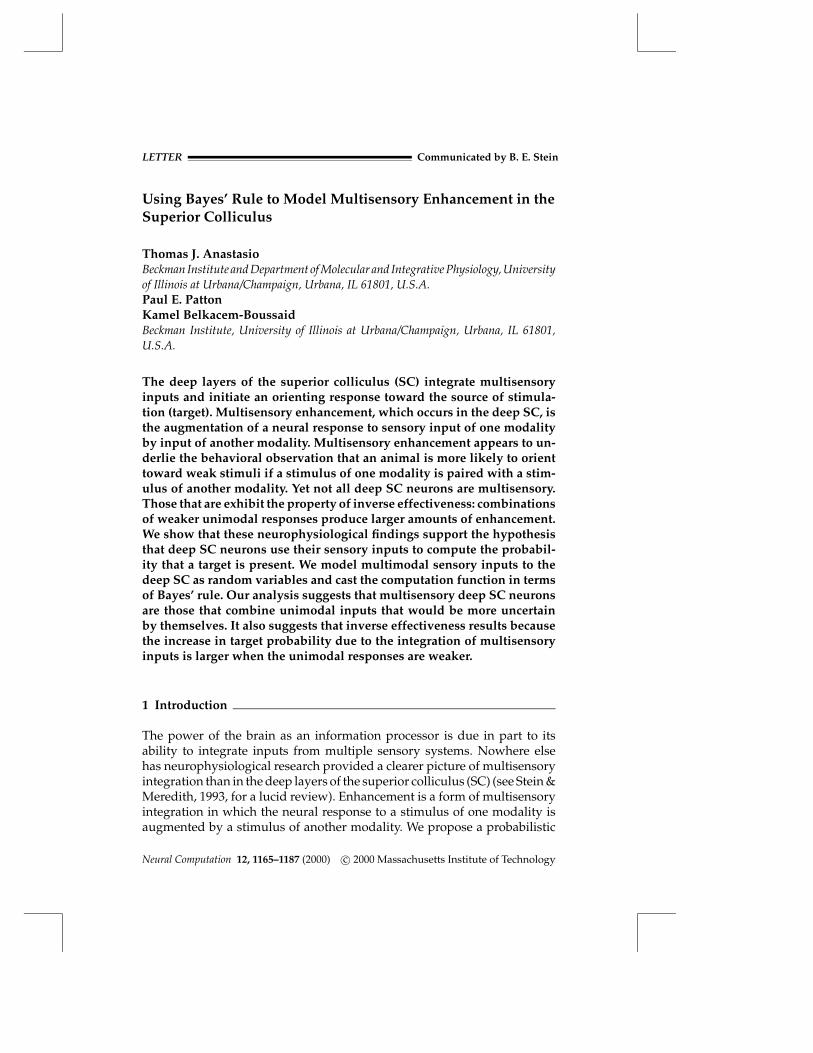
The model is schematized in Figure 1, in which the deep SC receives in-put from the visual and auditory systems. We represent these two sensorysystems because the bimodal, visual-auditory combination is the most com-mon one observed in cat and monkey (Wallace & Stein, 1996). The resultsgeneralize to any other combination. Each block on the grid in Figure 1 rep-resents a single, deep SC neuron. Our model will focus on individual deepSC neurons and on the visual and auditory inputs they receive from withintheir receptive fields.

We begin with the simplest case: a deep SC neuron receives an inputof only one sensory modality. We denote the target as random variable Tand a visual sensory input as random variable V. Then we hypothesizethat a deep SC neuron computes the conditional probability P(T | V). Thisconditional probability can be computed using Bayes’ rule (Hellstrom, 1984;Applebaum, 1996):

P(T | V) = P(V | T)P(T)P(V)

. (2.1)

Bayes’ rule is a fundamental concept in probability that has found wide ap-plication (Duda & Hart, 1973; Bishop, 1995). It underlies all modern systemsfor probabilistic inference in artificial intelligence (Russell & Norvig, 1995).


Figure 1: Schematic diagram illustrating multisensory integration in the deeplayers of the superior colliculus (SC). Neurons in the SC are organized topo-graphically according to the location in space of their receptive fields. Individualdeep SC neurons, represented as blocks on a grid, can receive sensory input ofmore than one modality. The receptive fields of individual multisensory neu-rons for inputs of different modalities overlap. V and A are random variablesrepresenting input from the visual and auditory systems, respectively. T is abinary random variable representing the target. P(T = 1 | V,A) is the Bayesianprobability that a target is present given sensory inputs V and A. The bird imageis from Stein and Meredith (1993).

We suggest that a deep SC neuron can be regarded as implementingBayes’ rule in computing the probability of a target given its sensory in-put. According to equation 2.1, we suppose that the nervous system cancompute P(T | V) given some input V because it already has available theother three probabilities: P(V | T), P(V), and P(T). The conditional prob-ability of V given T [P(V | T)] is the probability of obtaining some visualsensory input V = v given a target T = t (upper- and lowercase italicizedletters represent random variables and particular numerical values of thosevariables, respectively). In the context of Bayes’ rule, P(V | T) is referred toas the likelihood of V given T. The unconditional probability of V [P(V)]is the probability of obtaining some visual sensory input V = v regardlessof whether a target is present. Thus, P(V) and P(V | T) are properties ofthe visual system and the environment, and it is reasonable to suppose thatthose properties could be represented by the brain.


The unconditional probability of T [P(T)] is the probability that T = t.P(T) is a property of the environment. In the context of Bayes’ rule, P(T)is referred to as the prior probability of T. What Bayes’ rule essentiallydoes is to modify the prior probability on the basis of input. In Bayes’ rule(equation 2.1), P(T | V) is computed by multiplying P(T) by the ratio P(V |T)/P(V). Because P(T | V) can be thought of as a modified version of P(T)based on input, P(T | V) can be referred to as the posterior probability ofT. Thus, when computed using Bayes’ rule, P(T | V) is referred to as eitherthe Bayesian or the posterior probability of T. It’s possible that the priorprobability of T [P(T)], and its representation by the brain, could changeas circumstances dictate. With Bayes’ rule, we suggest a model of how thebrain could use knowledge of the statistical properties of its sensory systemsto modify this prior on the basis of sensory input.

3 Bayes’ Rule with One Sensory Input

Equation 2.1 can be used to compute the posterior (Bayesian) probability ofa target given sensory input of only one modality. It can be used to simu-late the responses of unimodal deep SC neurons. To evaluate equation 2.1,it is necessary to define the probability distributions for the terms on theright-hand side. We define T as a binary random variable where T = 1 ifthe target is present and T = 0 if it is absent. We define the prior prob-ability distribution of T [P(T)] by arbitrarily assigning the probability of0.1 to P(T = 1) and 0.9 to P(T = 0). These values are not meant to reflectprecisely some experimental situation, but are chosen because they offeradvantages in illustrating the principles. Bayes’ rule is valid for any priordistribution.

We define V as a discrete random variable that represents the numberof neural impulses arriving as input to a deep SC neuron from a visualneuron in a unit time interval. The unit interval for the data we model is250 msec (Meredith & Stein, 1986b). We define the likelihoods of V givenT = 1 [P(V | T = 1)] or T = 0 [P(V | T = 0)] as Poisson densities withdifferent means. The Poisson density provides a reasonable first approxi-mation to the discrete distribution of the number of impulses per unit timeobserved in the spontaneous activity and driven responses of single neu-rons, and offers certain modeling advantages. The Poisson density functionfor discrete random variable V with mean λ is defined as (Hellstrom, 1984;Applebaum, 1996):

P(V = v) = λve−λ

v!. (3.1)

Example likelihood distributions of V are illustrated in Figure 2A. Thelikelihood of V given T = 0 [P(V | T = 0)] is the probability distribution ofV when a target is absent. Thus, P(V | T = 0) is the likelihood of V under


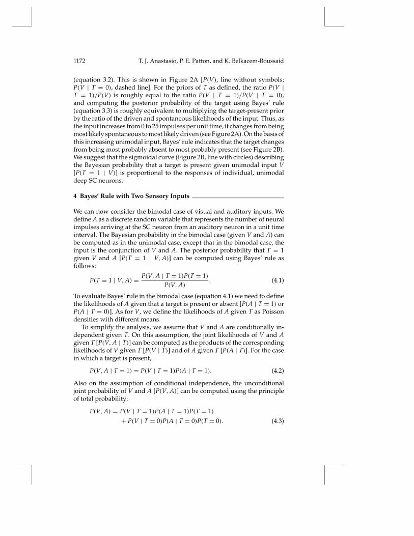
Figure 2: Likelihood distributions and Bayesian probability in the unimodalcase. The target is denoted by the binary random variable T. The prior prob-abilities of the target [P(T)] are 0.9 that it is absent [P(T = 0) = 0.9] and 0.1that it is present [P(T = 1) = 0.1]. The discrete random variable V representsthe number of impulses arriving at the deep SC from a visual input neuronin a unit time interval (250 msec). Poisson densities, shown in (A), model thelikelihood distributions of V [P(V | T)]. A mean 5 Poisson density models thespontaneous likelihood of V [with target absent, P(V | T = 0), dashed line]. Amean 8 Poisson density models the driven likelihood of V [with target present,P(V | T = 1), line with circles]. The unconditional probability of V [P(V), linewithout symbols in (A)] is computed from the input likelihoods and target pri-ors (using equation 3.2). The posterior (Bayesian) probability that the target ispresent given input V [P(T = 1 | V)] is computed using equation 3.3, and theresult is shown in (B) (line with circles). The target-present prior [P(T = 1) = 0.1]is also shown for comparison in (B) (dashed line).

spontaneous conditions. It is modeled as a Poisson density (equation 3.1)with λ = 5 (dashed line). The mean of 5 impulses per 250-msec intervalcorresponds to a mean spontaneous firing rate of 20 impulses per second.This spontaneous rate is meant to represent a reasonable generic value, butone that is high enough so that the behavior of the model under spontaneous


conditions can be examined easily. The model is valid for any spontaneousrate.

The likelihood of V given T = 1 [P(V | T = 1)] is the probability distribu-tion of V when a target is present. Thus, P(V | T = 1) is the likelihood of Vunder driven conditions. The driven likelihood takes into account randomvariability in the stimulus effectiveness of the target, as well as the intrin-sic stochasticity of the sensory neurons. It is modeled as a Poisson density(equation 3.1) with λ = 8 (line with circles in Figure 2A). The mean of 8 im-pulses per 250-msec interval corresponds to a mean driven firing rate of 32impulses per second. Notice that there is overlap between the spontaneousand driven likelihoods of V (see Figure 2A).

Given the prior probability distribution of T [P(T)] and the likelihooddistributions of V [P(V | T)], the unconditional probability of V [P(V)]can be computed using the principle of total probability (Hellstrom, 1984;Applebaum, 1996):

P(V) = P(V | T = 1)P(T = 1)+ P(V | T = 0)P(T = 0). (3.2)

Equation 3.2 shows that the unconditional probability of V is the sum of thelikelihoods of V weighted by the priors of T. The result is the compounddistribution shown in Figure 2A (line without symbols). With P(T) andP(V | T) defined, and P(V) computed from them (equation 3.2), all of thevariables needed to evaluate Bayes’ rule in the unimodal case (equation 2.1)have been specified.

Our hypothesis is that a deep SC neuron computes the Bayesian (poste-rior) probability that a target is present in its receptive field given its sensoryinput. We therefore want to evaluate equation 2.1 for T = 1 with unimodalinput V:

P(T = 1 | V) = P(V | T = 1)P(T = 1)P(V)

. (3.3)

We evaluate equation 3.3 by taking integer values of v in the range from 0to 25 impulses per unit time. For each value of v, the values of P(V | T = 1)and P(V) are read off the curves previously defined (see Figure 2A). Theunimodal posterior probability that T = 1 [P(T = 1 | V)] is plotted inFigure 2B (line with circles). The prior probability that T = 1 [P(T = 1) = 0.1]is also shown for comparison in Figure 2B (dashed line). For the Poissondensity means chosen, the posterior exceeds the prior probability whenv ≥ 7 impulses per unit time (see Figure 2B). For the same values of v(v ≥ 7), the driven likelihood of V [P(V | T = 1)] exceeds the unconditionalprobability of V [P(V)] (see Figure 2A).

Because the target-present prior [P(T = 1) = 0.1] is much smaller thanthe target-absent prior of T [P(T = 0) = 0.9], the unconditional probabilityof V [P(V)] is dominated by the spontaneous likelihood of V [P(V | T = 0)]


(equation 3.2). This is shown in Figure 2A [P(V), line without symbols;P(V | T = 0), dashed line]. For the priors of T as defined, the ratio P(V |T = 1)/P(V) is roughly equal to the ratio P(V | T = 1)/P(V | T = 0),and computing the posterior probability of the target using Bayes’ rule(equation 3.3) is roughly equivalent to multiplying the target-present priorby the ratio of the driven and spontaneous likelihoods of the input. Thus, asthe input increases from 0 to 25 impulses per unit time, it changes from beingmost likely spontaneous to most likely driven (see Figure 2A). On the basis ofthis increasing unimodal input, Bayes’ rule indicates that the target changesfrom being most probably absent to most probably present (see Figure 2B).We suggest that the sigmoidal curve (Figure 2B, line with circles) describingthe Bayesian probability that a target is present given unimodal input V[P(T = 1 | V)] is proportional to the responses of individual, unimodaldeep SC neurons.

4 Bayes’ Rule with Two Sensory Inputs

We can now consider the bimodal case of visual and auditory inputs. Wedefine A as a discrete random variable that represents the number of neuralimpulses arriving at the SC neuron from an auditory neuron in a unit timeinterval. The Bayesian probability in the bimodal case (given V and A) canbe computed as in the unimodal case, except that in the bimodal case, theinput is the conjunction of V and A. The posterior probability that T = 1given V and A [P(T = 1 | V,A)] can be computed using Bayes’ rule asfollows:

P(T = 1 | V,A) = P(V,A | T = 1)P(T = 1)P(V,A)

. (4.1)

To evaluate Bayes’ rule in the bimodal case (equation 4.1) we need to definethe likelihoods of A given that a target is present or absent [P(A | T = 1) orP(A | T = 0)]. As for V, we define the likelihoods of A given T as Poissondensities with different means.

To simplify the analysis, we assume that V and A are conditionally in-dependent given T. On this assumption, the joint likelihoods of V and Agiven T [P(V,A | T)] can be computed as the products of the correspondinglikelihoods of V given T [P(V | T)] and of A given T [P(A | T)]. For the casein which a target is present,

P(V,A | T = 1) = P(V | T = 1)P(A | T = 1). (4.2)

Also on the assumption of conditional independence, the unconditionaljoint probability of V and A [P(V,A)] can be computed using the principleof total probability:

P(V,A) = P(V | T = 1)P(A | T = 1)P(T = 1)

+ P(V | T = 0)P(A | T = 0)P(T = 0). (4.3)


We use the same priors of T as before. With the priors of T and the like-lihoods of V and A defined, and the conditional and unconditional jointprobabilities of (V,A) computed from them (equations 4.2 and 4.3), we canuse Bayes’ rule (equation 4.1) to simulate the bimodal responses of deepSC neurons. We evaluate equation 4.1 by taking integer values of v and ain the range from 0 to 25 impulses per unit time. To simplify the compari-son between simulated unimodal and bimodal responses, we consider thehypothetical case in which v and a are equal. The results are qualitativelysimilar when v and a are unequal as long as they increase together.

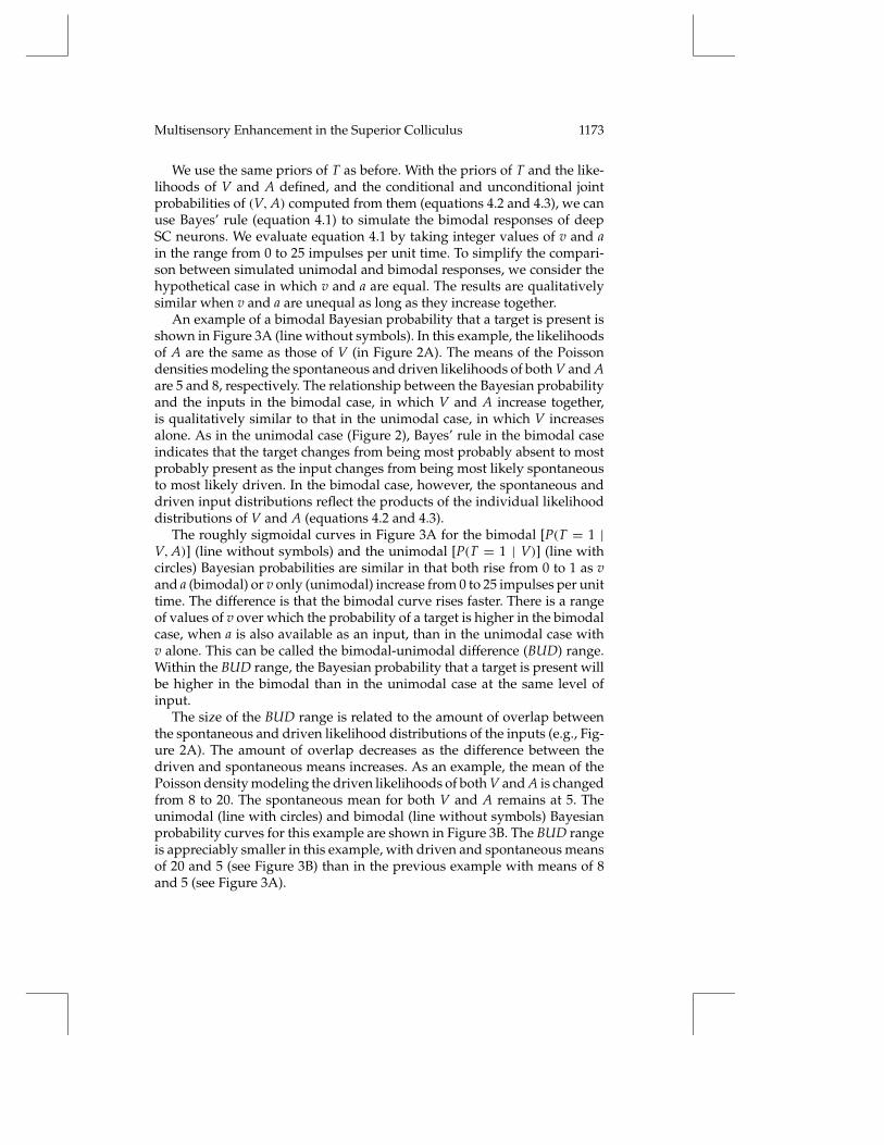
An example of a bimodal Bayesian probability that a target is present isshown in Figure 3A (line without symbols). In this example, the likelihoodsof A are the same as those of V (in Figure 2A). The means of the Poissondensities modeling the spontaneous and driven likelihoods of both V and Aare 5 and 8, respectively. The relationship between the Bayesian probabilityand the inputs in the bimodal case, in which V and A increase together,is qualitatively similar to that in the unimodal case, in which V increasesalone. As in the unimodal case (Figure 2), Bayes’ rule in the bimodal caseindicates that the target changes from being most probably absent to mostprobably present as the input changes from being most likely spontaneousto most likely driven. In the bimodal case, however, the spontaneous anddriven input distributions reflect the products of the individual likelihooddistributions of V and A (equations 4.2 and 4.3).

The roughly sigmoidal curves in Figure 3A for the bimodal [P(T = 1 |V,A)] (line without symbols) and the unimodal [P(T = 1 | V)] (line withcircles) Bayesian probabilities are similar in that both rise from 0 to 1 as vand a (bimodal) or v only (unimodal) increase from 0 to 25 impulses per unittime. The difference is that the bimodal curve rises faster. There is a rangeof values of v over which the probability of a target is higher in the bimodalcase, when a is also available as an input, than in the unimodal case withv alone. This can be called the bimodal-unimodal difference (BUD) range.Within the BUD range, the Bayesian probability that a target is present willbe higher in the bimodal than in the unimodal case at the same level ofinput.

The size of the BUD range is related to the amount of overlap betweenthe spontaneous and driven likelihood distributions of the inputs (e.g., Fig-ure 2A). The amount of overlap decreases as the difference between thedriven and spontaneous means increases. As an example, the mean of thePoisson density modeling the driven likelihoods of both V and A is changedfrom 8 to 20. The spontaneous mean for both V and A remains at 5. Theunimodal (line with circles) and bimodal (line without symbols) Bayesianprobability curves for this example are shown in Figure 3B. The BUD rangeis appreciably smaller in this example, with driven and spontaneous meansof 20 and 5 (see Figure 3B) than in the previous example with means of 8and 5 (see Figure 3A).


Figure 3: Bayesian target-present probabilities computed in unimodal and bi-modal cases. The prior probabilities of the target are set as before [P(T = 1) = 0.1and P(T = 0) = 0.9] and the likelihoods of the visual (V) and auditory (A) in-puts are modeled using Poisson densities as in Figure 2A. Unimodal Bayesianprobabilities (see equation 3.3) are computed as V takes integer values v in therange from 0 to 25 impulses per unit time. Bimodal Bayesian probabilities (equa-tion 4.1) are computed as V and A vary together over the same range with v = a.(A) Spontaneous and driven likelihood means are 5 and 8, respectively, for theunimodal case of V only, and for both V and A in the bimodal case. (B) Spon-taneous and driven likelihood means are 5 and 20, respectively. The bimodalexceeds the unimodal Bayesian probability over a much narrower range in (B)than in (A). For (A) and (B), lines with circles and lines without symbols denoteunimodal and bimodal Bayesian probabilities, respectively.

Comparison of the curves in Figures 3A and 3B illustrates the generalfinding that the BUD range decreases as the difference between the drivenand spontaneous input means increases. The BUD range is also dependenton the prior probabilities of the target. The influences of changing the spon-taneous and driven input means and target priors on the BUD range areillustrated in Figure 4. In this figure, the summed difference between thebimodal and unimodal Bayesian probability curves (cumulative BUD) is


Figure 4: The difference between the bimodal and unimodal Bayesian proba-bilities decreases rapidly as the difference between the driven and spontaneousinput means increases. The spontaneous means for both V and A are fixed at 5impulses per unit time, and the driven means for V and A are varied togetherfrom 7 to 25. Unimodal (equation 3.3) and bimodal (equation 4.1) Bayesian prob-abilities are computed as v, or v and a together, vary over the range from 0 to25 impulses per unit time (as in Figure 3). The unimodal is subtracted fromthe bimodal curve at each point in the input range. The difference (BUD) issummed over the range and plotted. The cumulative BUD is computed withtarget-present prior probabilities of 0.1 (line without symbols), 0.01 (dashedline), and 0.001 (line with asterisks) (target-absent priors are 0.9, 0.99, and 0.999,respectively).


plotted as the driven means of both V and A are varied together from 7to 25. The spontaneous means of both V and A are fixed at 5. The targetprior distribution is altered so that the target-present prior equals 0.1 (linewithout symbols), 0.01 (dashed line), or 0.001 (line with asterisks). Figure 4shows that the cumulative BUD decreases as the difference between thedriven and spontaneous input means increases. The difference is higher forall means as the target-present prior decreases.

Whether a deep SC neuron receives multimodal or only unimodal inputmay depend on the amount by which the driven response of a unimodalinput differs from its spontaneous discharge. If the spontaneous and drivenmeans are not well separated, then a unimodal sensory input provided toa deep SC neuron indicating the presence of a target would be uncertainand ambiguous. In the ambiguous case, a sensory input of another modal-ity makes a relatively big difference in the computation of the probabilitythat a target is present (e.g., Figure 4 for driven means less than about 15).Conversely, if the spontaneous and driven means are well separated, thena unimodal input provided to a deep SC neuron would be unambiguous.In the unambiguous case, a sensory input of another modality makes rela-tively little difference in the computation of the probability that a target ispresent (e.g., Figure 4 for driven means greater than about 15). Unimodaldeep SC neurons may be those that receive an unambiguous input of onesensory modality and have no need for an input of another modality.

5 Bayes’ Rule with One Spontaneous and One Driven Input

To compare the Bayes’ rule model with neurophysiological data on multi-sensory enhancement, we must explore the behavior of the bimodal model(equation 4.1) not only for cases of bimodal stimulation, but also for caseswhere stimulation of only one or the other modality is available. To modelthe experimental situation in which sensory stimulation of both modalitiesis presented, we consider the case in which v and a are equal and vary to-gether over the range from 0 to 25 impulses per unit time (as before). Thissimulates the driven responses of both inputs (both-driven). To model situ-ations in which sensory stimulation of only one modality is presented, weconsider the cases in which v or a is allowed to vary over the range, while theother input is fixed at the mean of its spontaneous likelihood distribution(driven/spontaneous).

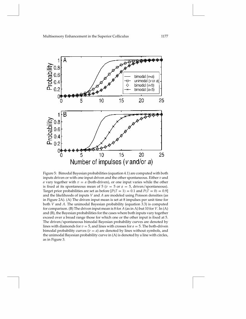
The results of these simulations are shown in Figure 5A, in which thespontaneous and driven input means are 5 and 8 for both V and A, as before.Because both sensory inputs have the same spontaneous and driven means,the bimodal Bayesian probability curves for the two driven/spontaneouscases are the same. Thus, the curves coincide for the bimodal cases in whichv is fixed at 5 while a varies (line with diamonds) and in which a is fixedat 5 while v varies (line with crosses). There is a range of v and a in Fig-ure 5A over which the bimodal Bayesian probability in the both-driven


Figure 5: Bimodal Bayesian probabilities (equation 4.1) are computed with bothinputs driven or with one input driven and the other spontaneous. Either v anda vary together with v = a (both-driven), or one input varies while the otheris fixed at its spontaneous mean of 5 (v = 5 or a = 5, driven/spontaneous).Target prior probabilities are set as before [P(T = 1) = 0.1 and P(T = 0) = 0.9]and the likelihoods of inputs V and A are modeled using Poisson densities (asin Figure 2A). (A) The driven input mean is set at 8 impulses per unit time forboth V and A. The unimodal Bayesian probability (equation 3.3) is computedfor comparison. (B) The driven input mean is 8 for A (as in A) but 10 for V. In (A)and (B), the Bayesian probabilities for the cases where both inputs vary togetherexceed over a broad range those for which one or the other input is fixed at 5.The driven/spontaneous bimodal Bayesian probability curves are denoted bylines with diamonds for v = 5, and lines with crosses for a = 5. The both-drivenbimodal probability curves (v = a) are denoted by lines without symbols, andthe unimodal Bayesian probability curve in (A) is denoted by a line with circles,as in Figure 3.


case (line without symbols) exceeds that in the driven/spontaneous cases(lines with diamonds and crosses). This can be called the range of enhance-ment.

The bimodal curves (both-driven and driven/spontaneous; equation 4.1)are compared in Figure 5A with the corresponding unimodal Bayesian prob-ability curve computed before (equation 3.3). It shows that the Bayesianprobabilities in the bimodal, driven/spontaneous cases (lines with dia-monds and crosses) are smaller than in the unimodal case (line with circles)for the same inputs v and/or a. This illustrates that Bayes’ rule works inboth directions. The bimodal probability can be higher than the unimodalprobability when the target most likely drives both inputs. Conversely, thebimodal probability can be lower than the unimodal probability when thetarget most likely drives one input while the other input is most likely spon-taneous.

For simplicity, we have considered cases of the bimodal Bayes’ rule wherethe likelihood distributions are the same for inputs of both modalities. TheBayesian analysis presented is valid for any input mean values, as long asinputs that are intended to represent neurons that are activated by sensorystimulation have driven means that are higher than spontaneous means.Figure 5B presents an example of bimodal Bayesian probabilities computedwith the same spontaneous means (of 5), but with different driven meansof 10 and 8 for V and A, respectively. This case is qualitatively similar to theprevious one except that the driven/spontaneous curves do not coincide.The range of enhancement is much larger relative to the curve for which avaries alone while v = 5 (line with diamonds) than relative to the curve forwhich v varies alone while a = 5 (line with crosses). There are values of theinput for which a driven/spontaneous probability is almost zero while theboth-driven probability is almost one.

We hypothesize that the response of a deep SC neuron is proportionalto the Bayesian probability that a target is present given its inputs. Forthe curves in Figures 5A and 5B, the ranges of input over which the bi-modal, both-driven probabilities (lines without symbols) exceed the driven/spontaneous probabilities (lines with diamonds and crosses) correspond toranges of multisensory enhancement. As v and a increase within a rangeof enhancement, the amount of enhancement increases and then decreasesuntil, above the upper limit of the range, enhancement decreases to zero.This behavior of the bimodal Bayes’ rule model can be used to simulate theresults of a neurophysiological experiment (Meredith & Stein, 1986b).

The experiment involves recording the responses of a multisensory deepSC neuron to stimuli that by themselves produce minimal, suboptimal, oroptimal responses. The simulation is based on the bimodal case shown inFigure 5B, in which the driven means for V and A are different. Inputsfor v and a are chosen that give similar minimal, suboptimal, and opti-mal Bayesian probabilities in the driven/spontaneous case. The both-drivenprobability is computed using the same, driven input values. The percent-


Table 1: Numerical Values for a Simulated Enhancement Experiment.

Driven Input Bimodal Bayesian Probability

v a v Driven a Driven va Driven % enh

Minimal 8 9 0.0476 0.0487 0.3960 713Suboptimal 12 15 0.4446 0.4622 0.9865 113Optimal 16 21 0.9276 0.9351 1 7

Notes: Target prior probabilities are set at 0.1 for target present and 0.9 for target absent.The likelihoods of inputs V and A are modeled using Poisson densities with a spontaneousmean of 5 impulses per unit time for both V and A and driven means of 10 for V and 8for A. With one input fixed at the spontaneous mean, the other input (v or a) is assigneda driven value such that the two driven/spontaneous, bimodal Bayesian probabilitiesare approximately equal at each of three levels (minimal, suboptimal, and optimal). Theboth-driven (va) bimodal Bayesian probability is computed using the same driven inputvalues. The percentage enhancement is computed using equation 1.1 in which the both-driven probability is substituted for CM and the larger of the two driven/spontaneousprobabilities is substituted for SMmax. The percentage increase in the Bayesian probability(% enh, equation 1.1) when both inputs are driven is largest when the driven/spontaneousBayesian probabilities are smallest.

age enhancement is computed using equation 1.1, in which the Bayesian,bimodal both-driven probability is substituted for CM and the larger of thetwo driven/spontaneous probabilities is substituted for SMmax. The valuesare listed in Table 1.

The results are illustrated in Figure 6, where the bars correspond to theBayesian, bimodal probabilities in the driven/spontaneous cases (white bar,visual driven (v); gray bar, auditory driven (a)) or in the both-driven case(black bar, visual and auditory driven (va)). Figure 6 is drawn as a bar graphto facilitate comparisons with published figures based on experimental data(Meredith & Stein, 1986b; Stein & Meredith, 1993). Figure 6 shows that in themodel, the percentage enhancement goes down as the driven/spontaneousprobabilities go up. These modeling results simulate the property of inverseeffectiveness that is observed for multisensory deep SC neurons, by whichthe percentage of multisensory enhancement is largest when the single-modality responses are smallest.

6 Discussion

Multisensory enhancement is a particularly dramatic form of multisensoryintegration in which the response of a deep SC neuron to a stimulus of onemodality can be increased many times by a stimulus of another modality.Yet not all deep SC neurons are multisensory. Those that are exhibit theproperty of inverse effectiveness, by which the percentage of multisensoryenhancement is largest when the single-sensory responses are smallest. Wehypothesize that the responses of individual deep SC neurons are propor-


Figure 6: Comparing the driven/spontaneous bimodal Bayesian probabilitiesat three levels (minimal, suboptimal, and optimal) with the corresponding both-driven probability. Parameters for the target prior and input likelihood distri-butions are as in Figure 5B. Bimodal probabilities (equation 4.4) are computedwhen both v and a take various values within the range representing driven re-sponses (va, black bars), or when one input takes the driven value (v, white bars;a, gray bars) but the other is fixed at the spontaneous mean of 5. The percent-age increase in the Bayesian probability when both inputs are driven is largestwhen the driven/spontaneous Bayesian probabilities are smallest. The valuesare reported in Table 1.

tional to the Bayesian probability that a target is present given their sensoryinputs. Our model, based on this hypothesis, suggests that multisensorydeep SC neurons are those that receive unimodal inputs that would bemore ambiguous by themselves. It also provides an explanation for theproperty of inverse effectiveness. The probability of a target computed onthe basis of a large unimodal input will not be increased much by an inputof another modality. However, the increase in target probability due to theintegration of inputs of two modalities goes up rapidly as the size of theunimodal inputs decreases. Thus, our hypothesis provides a functional in-terpretation of multisensory enhancement that can explain its most salientfeatures.


6.1 Hypothesis, Assumptions, and Model Parameters. Our basic hy-pothesis is that the responses of deep SC neurons are proportional to theprobability that a target is present. A similar hypothesis was put forwardby Barlow (1969, 1972), who suggested that the responses of feature detec-tor neurons are proportional to the probability that their trigger feature ispresent. Barlow suggested a model based on classical statistical inference,in which the response of a neuron is proportional to− log(P)where P is theprobability of the results on a null hypothesis (i.e., that the trigger feature isabsent). Classical inference differs from Bayesian analysis in many respects,with the main difference being that prior information is used in the latter butnot in the former (Applebaum, 1996). In our model, the response of a deepSC neuron is directly proportional to the Bayesian (posterior) probability ofa target, based on the prior probability of the target and sensory input ofone or more modalities.

We constructed our model so as to minimize the number of assumptionsneeded to evaluate it. That was our motivation in choosing the Poissondensity rather than some other probability density function to represent thevisual and auditory inputs, and in considering those two inputs as con-ditionally independent given the target. The Bayesian formulation is validregardless of the probability density function chosen to represent the inputs,or whether those inputs are independent or dependent. Our particular con-struction of the model demonstrates its robustness, since the parameters ofother instantiations requiring additional assumptions can easily be set soas to exaggerate the multisensory enhancement effects that we successfullysimulate despite the constraints we impose.

Conditional independence given the target implies that the visibility of atarget indicates nothing about its audibility, and vice-versa. One can easilyimagine real targets for which this assumption is valid and others for whichit is not. The advantage of the assumption of conditional independence isthat the conditional and unconditional joint distributions of the visual andauditory inputs [P(V,A | T) and P(V,A)] are then computed directly fromthe likelihoods of each individual input and the target priors (equations 4.2and 4.3). The alternative assumption of conditional dependence carries withit a number of additional assumptions that would have to be made in orderto specify how V and A are jointly distributed. The parameters of such a de-pendent, joint distribution could not be constrained on the basis of availabledata, but could be chosen in such a way that the simulated multisensoryenhancement effects would be greatly exaggerated. Thus, our model con-struction based on conditional independence of the inputs is more restrictivethan the dependent alternative, and conclusions based on it are thereforestronger.

The spike trains of individual neurons have been described using vari-ous stochastic processes (Gerstein & Mandelbrot, 1964; Geisler & Goldberg,1966; Lansky & Radil, 1987; Gabbiani & Koch, 1998). We use the discretePoisson density to approximate the number of impulses per unit time in


the discharge of individual neurons. Real spike trains can be well describedas Poisson processes in some cases but not in others (Munemori, Hara,Kimura, & Sato, 1984; Turcott et al., 1994; Lestienne, 1996; Rieke, Warland,& de Ruyter van Stevenick, 1997). The advantage of the Poisson density isthat it is specified using only one parameter, the mean, and this parame-ter has been reported for neurons in many of the brain regions that supplysensory input to the deep SC. Other densities require setting two or more pa-rameters, which could not be well constrained on the basis of available databut could be chosen in such a way that the simulated multisensory enhance-ment effects would be greatly exaggerated. Thus, our model constructionusing Poisson densities to represent the inputs is better constrained thanothers that would use alternative densities, and conclusions based on it aretherefore more robust.

6.2 Unimodality versus Bimodality. Our analysis suggests that whethera deep SC neuron is multisensory may depend on the statistical propertiesof its inputs. We use two probability distributions to define each sensoryinput: one for its spontaneous discharge and the other for its activity as it isdriven by the sensory attributes of the target. A critical feature of these dis-tributions is their degree of overlap. The more the spontaneous and drivendistributions of an input overlap, the more uncertain and ambiguous willthat input be for indicating the presence of a target.

Our model suggests that if a deep SC neuron receives a unimodal in-put for which the spontaneous and driven distributions have little overlap,then that neuron receives unambiguous unimodal input and has no needfor input of another modality. Conversely, if a deep SC neuron receives aunimodal input for which the spontaneous and driven distributions over-lap a lot, then that neuron receives ambiguous unimodal input. Such a deepSC neuron could effectively disambiguate this input by combining it withan input of another modality, even if the other input is also ambiguous byitself. About 45% of deep SC neurons in the cat and 21% in the monkey re-ceive input from two sensory modalities (Wallace & Stein, 1996). An inputof a third modality could provide further disambiguation. About 9% of alldeep SC neurons in the cat and 6% in the monkey receive input of threemodalities. Inputs to the deep SC are likely to vary in the degree to whichtheir spontaneous discharges and driven responses overlap. For example,sensory neurons vary in their sensitivity, and overlap would occur for thosethat are less sensitive to stimulation. Sensory inputs would therefore varyin their degree of ambiguity. This could explain why some deep SC neuronsare unimodal while others are multimodal (Wallace & Stein, 1996).

6.3 Spontaneous Activity. In the model, the Bayesian probability of atarget increases from zero to one as the input increases. We suggest that theresponses of individual deep SC neurons are proportional to this Bayesianprobability. The Bayesian probability is zero or nearly zero for inputs that are


most likely spontaneous. For the example shown in Figure 2, the Bayesianprobability is nearly zero even for an input of 16 impulses per second(4 impulses per 250-msec interval). The spontaneous activity of deep SCneurons is also zero or nearly zero, despite the fact that most of the neu-rons that supply input to the deep SC have nonzero spontaneous firingrates.

The spontaneous rates of neurons in some of the cortical and subcor-tical visual and auditory regions that project to the deep SC range fromzero to over 100 impulses per second (anterior ectosylvian visual area inanesthetized cat, 1–8 Hz: Mucke, Norita, Benedek, & Creutzfeldt, 1982; pre-tectum in anesthetized cat, 1–31 Hz: Schmidt, 1996; retinal ganglion cells inanesthetized cat, 0–80 Hz: Ikeda, Dawes, & Hankins, 1992; superior olivarycomplex in anesthetized cat, 0–140 Hz: Guinan, Guinan, & Norris, 1972; infe-rior colliculus in alert cat, 2–54 Hz: Bock, Webster, & Aitkin, 1971; trapezoidbody in anesthetized cat, 0–104 Hz: Brownell, 1975). For the unanesthetizedrabbit, mean spontaneous rates of 36.1± 37.8 (SD) and 11.1± 11.4 (SD) im-pulses per second have been observed for single neurons in the superiorolivary complex and inferior colliculus, respectively (D. Fitzpatrick andS. Kuwada, pers. comm.). Although neurons discharge spontaneously inmost of the regions that provide inputs to the deep SC, most deep SC neu-rons exhibit low or zero spontaneous discharge, in both the anesthetizedpreparation and the alert, behaving animal (Peck, Schlag-Rey, & Schlag,1980; Middlebrooks & Knudsen, 1984; Grantyn & Berthoz, 1985). In thecontext of the model, we would interpret this low level of deep SC neuronactivity as indicating that the probability of a target is low when the inputsare spontaneous.

6.4 Driven Responses. The driven responses of deep SC neurons areinfluenced by a multidimensional array of stimulus parameters in additionto location in space. For visual stimuli these can include size, and rate anddirection of motion (Stein & Arigbede, 1972; Gordon, 1973; Peck et al., 1980;Wallace & Stein, 1996). For auditory stimuli, factors influencing driven re-sponses include sound frequency, intensity, and motion of the sound source(Gordon, 1973; Wise & Irvine, 1983, 1985; Hirsch, Chan, & Yin, 1985; Yin,Hirsch, & Chan, 1985). Specificity for these parameters is most likely de-rived from the sensory systems that provide input to the deep SC. In themodel, we represent input activity as the number of impulses per unit time,which increases monotonically as the optimality of the sensory stimulus in-creases. The multidimensional array of stimulus parameters, as well as themultiplicity of input sources, raises the possibility of enhancement within asingle sensory modality. For example, a visual input specific for size mightenhance another visual input specific for direction of motion. The basicmodel, which includes only one input from each of two sensory modalities,can be generalized to include arbitrarily many inputs of various modalitiesand specificities.


The Bayesian probability increases as the input increases, and is one ornearly one for inputs that are most likely driven. A Bayesian probability ofone could correspond to the maximum activity level of deep SC neurons.The model suggests that unimodal input could maximally drive individualdeep SC neurons, even those that are multisensory (e.g., Figure 5). However,in order for some inputs to drive deep SC neurons maximally, they wouldhave to attain very high activity levels. For example, when the auditoryinput alone is driven in Figure 5B (line with diamonds), it does not producea Bayesian probability of one even when it has attained 80 impulses persecond (20 impulses per unit time). It is possible that some unimodal inputsare unable to attain the activity levels needed to drive deep SC neuronsmaximally, regardless of the optimality of the unimodal stimulus. The max-imal response of a multimodal neuron to such unimodal input would beless than its maximal bimodal or multimodal response. Neurophysiologicalevidence suggests that this may be the case for some deep SC neurons (Stein& Meredith, 1993).

6.5 Multisensory Enhancement and Inverse Effectiveness. When theresponses of deep SC neurons are interpreted as being proportional to theBayesian probability of a target, then multisensory enhancement is analo-gous to an increase in that probability due to multimodal input. The strengthof the evidence of a target provided to a deep SC neuron is related to thesize of its driven input. If a driven input of one modality is large, a deep SCneuron receives overwhelming evidence on the basis of that input modal-ity alone. The probability of a target would be high, and driven input ofanother modality will not increase that probability much. Conversely, if adriven input of one modality is small, then the evidence it provides to adeep SC neuron is weak, and the probability of a target computed on thebasis of that input alone would be small. In that case, the probability of a tar-get could be greatly increased by corroborating input of another modality.According to the probabilistic interpretation, the amount of multisensoryenhancement should be larger for smaller unimodal inputs.

The experimental paradigm actually used to demonstrate multisensoryenhancement would accentuate this effect. Typically in studying a multisen-sory deep SC neuron, the response to stimuli of two modalities presentedtogether is compared with the response to a stimulus of either modality pre-sented alone (Meredith & Stein, 1986b; Stein & Meredith, 1993). Accordingto the model, the response of a bimodal, deep SC neuron to a unimodal stim-ulus would be proportional to the probability of a target given that one inputis driven and the other is spontaneous. This bimodal, driven/spontaneousprobability is lower than that which would be computed by a unimodal deepSC neuron receiving only the driven input (see Figure 5A). The both-drivenbimodal probability can be increased greatly over the driven/spontaneousbimodal probabilities, especially when the driven/spontaneous probabili-ties are smaller.


Thus, the amount of increase in target probability due to the integrationof multimodal sensory inputs goes up rapidly as the responses to unimodalinputs decrease. This relationship is illustrated in Figures 5 and 6. It is anal-ogous to the phenomenon of inverse effectiveness, which is the hallmarkof multisensory enhancement in deep SC neurons (Stein & Meredith, 1993).The property of inverse effectiveness is precisely what would be expectedon the basis of the hypothesis that deep SC neurons use their multisensoryinputs to compute the probability of a target.

Acknowledgments

We thank Pierre Moulin, Hao Pan, Sylvian Ray, Jesse Reichler, and Christo-pher Seguin for many helpful discussions and for comments on the manu-script prior to submission. This work was supported by NSF grant IBN92-21823 and a grant from the Critical Research Initiatives of the State ofIllinois, both to T.J.A.

References

Applebaum, D. (1996). Probability and information: An integrated approach. Cam-bridge: Cambridge University Press.

Barlow, H. B. (1969). Pattern recognition and the responses of sensory neurons.Annals of the New York Academy of Sciences, 156, 872–881.

Barlow, H. B. (1972). Single units and sensation: A neuron doctrine for perceptualpsychology? Perception, 1, 371–394.

Bishop, C. M. (1995). Neural networks for pattern recognition. Oxford: ClarendonPress.

Bock, G. R., Webster, W. R., & Aitkin, L. M. (1971). Discharge patterns of singleunits in inferior colliculus of the alert cat. J. Neurophysiol., 35, 265–277.

Brownell, W. E. (1975). Organization of the cat trapezoid body and the dischargecharacteristics of its fibers. Brain Res., 94(3), 413–433.

Cadusseau, J., & Roger, M. (1985). Afferent projections to the superior colliculusin the rat, with special attention to the deep layers. J. Hirnforsch., 26(6), 667–681.

Duda, R. O., & Hart, P. E. (1973). Pattern classification and scene analysis. NewYork: Wiley.

Edwards, S. B., Ginsburgh, C. L., Henkel, C. K., & Stein, B. E. (1979). Sources ofsubcortical projections to the superior colliculus in the cat. J. Comp. Neurol.,184(2), 309–329.

Gabbiani, F., & Koch, C. (1998). Principles of spike train analysis. In C. Koch &I. Segev (Eds.), Methods in neuronal modeling (2nd ed.). (pp. 312–360). Cam-bridge, MA: MIT Press.

Geisler, C. D., & Goldberg, J. M. (1966). A stochastic model of the repetitiveactivity of neurons. Biophys. J., 6, 53–69.

Gerstein, G. L., & Mandelbrot, B. (1964). Random walk models for the spikeactivity of a single neuron. Biophys. J., 4, 41–68.


Gordon, B. (1973). Receptive fields in deep layers of cat superior colliculus. J.Neurophysiol., 36(2), 157–178.

Grantyn, A., & Berthoz, A. (1985). Burst activity of identified tecto-reticulo-spinal neurons in the alert cat. Exp. Brain Res., 57(2), 417–421.

Guinan, J. J., Guinan, S. S., & Norris, B. E. (1972). Single auditory units in thesuperior olivary complex. I. Responses to sounds and classifications basedon physiological properties. Int. J. Neurosci., 4, 101–120.

Hellstrom, C. W. (1984). Probability and stochastic processes for engineers. New York:Macmillan.

Hirsch, J. A., Chan, J. C., & Yin, T. C. (1985). Responses of neurons in the cat’ssuperior colliculus to acoustic stimuli. I. Monaural and binaural responseproperties. J. Neurophysiol., 53(3), 726–745.

Ikeda, H., Dawes, E., & Hankins, M. (1992). Spontaneous firing level distiguishesthe effects of NMDA and non-NMDA receptor antagonists on the ganglioncells in the cat retina. Eur. J. Pharm., 210, 53–59.

King, A. J., & Palmer, A. R. (1985). Integration of visual and auditory informationin bimodal neurones in guinea-pig superior colliculus. Exp. Brain Res., 60,492–500.

Lansky, P., & Radil, T. (1987). Statistical inference on spontaneous neuronal dis-charge patterns. Biol. Cybern., 55, 299–311.

Lestienne, R. 1996. Determination of the precision of spike timing in the visualcortex of anaesthetised cats. Biol. Cybern., 74, 55–61.

Meredith, M. A., Clemo, H. R., & Stein, B. E. (1991). Somatotopic component ofthe multisensory map in the deep laminae of the cat superior colliculus. J.Comp. Neurol., 312(3), 353–370.

Meredith, M. A., Nemitz, J. W., & Stein, B. E. (1987). Determinants of mul-tisensory integration in superior colliculus neurons. I. Temporal factors. J.Neurosci., 7(10), 3215–3229.

Meredith, M. A., & Stein, B. E. (1983). Interactions among converging sensoryinputs in the superior colliculus. Science, 221(4608), 389–391.

Meredith, M. A., & Stein, B. E. (1986a). Spatial factors determine the activityof multisensory neurons in cat superior colliculus. Brain Res., 365(2), 350–354.

Meredith, M. A., & Stein, B. E. (1986b). Visual, auditory, and somatosensory con-vergence on cells in superior colliculus results in multisensory integration. J.Neurophysiol., 56(3), 640–662.

Meredith, M. A., & Stein, B. E. (1990). The visuotopic component of the multi-sensory map in the deep laminae of the cat superior colliculus. J. Neurosci.,10(11), 3727–3742.

Meredith, M. A., & Stein, B. E. (1996). Spatial determinants of multisensoryintegration in cat superior colliculus neurons. J. Neurophysiol., 75(5), 1843–1857.

Middlebrooks, J. C., & Knudsen, E. I. (1984). A neural code for auditory spacein the cat’s superior colliculus. J. Neurosci., 4(10), 2621–2634.

Mucke, L., Norita, M., Benedek, G., & Creutzfeldt, O. (1982). Physiologic andanatomic investigation of a visual cortical area situated in the ventral bankof the anterior ectosylvian sulcus of the cat. Exp. Brain Res., 46, 1–11.


Munemori, J., Hara, K., Kimura, M., & Sato, R. (1984). Statistical features ofimpulse trains in cat’s lateral geniculate neurons. Biol. Cybern., 50, 167–172.

Peck, C. K., Schlag-Rey, M., & Schlag, J. (1980). Visuo-oculomotor properties ofcells in the superior colliculus of the alert cat. J. Comp. Neurol., 194(1), 97–116.

Rieke, F., Warland, D., & de Ruyter van Stevenick, R. (1997). Spikes: Exploring theneural code. Cambrige, MA: MIT Press.

Russell, S., & Norvig, P. (1995). Artificial intelligence: A modern approach. UpperSaddle River, NJ: Prentice Hall.

Schmidt, M. (1996). Neurons in the cat pretectum that project to the dorsal lateralgeniculate nucleus are activated during saccades. J. Neurophysiol., 76(5), 2907–2918.

Sparks, D. L., & Hartwich-Young, R. (1989). The deep layers of the superiorcolliculus. In R. H. Wurtz & M. Goldberg (Eds.), The neurobiology of saccadiceye movements (pp. 213–255). Amsterdam: Elsevier.

Stein, B. E., & Arigbede, M. O. (1972). A parametric study of movement detectionproperties of neurons in the cat’s superior colliculus. Brain Res., 45, 437–454.

Stein, B. E., Huneycutt, W. S., & Meredith, M. A. (1988). Neurons and behavior:The same rules of multisensory integration apply. Brain Res., 448(2), 355–358.

Stein, B. E., & Meredith, M. A. (1993). The merging of the senses. Cambridge, MA:MIT Press.

Stein, B. E., Meredith, M. A., Huneycutt, W. S., & McDade, L. (1989). Behavioralindices of multisensory integration: Orientation to visual cues is affected byauditory stimuli. J. Cog. Neurosci., 1(1), 12–24.

Turcott, R. G., Lowen, S. B., Li, E., Johnson, D. H., Tsuchitani, C., & Teich, M.C. (1994). A non-stationary Poisson point process describes the sequenceof action potentials over long time scales in lateral-superior-olive auditoryneurons. Biol. Cybern., 70, 209–217.

Wallace, M. T., & Stein, B. E. (1994). Cross-modal synthesis in the midbraindepends on input from cortex. J. Neurophysiol., 71(1), 429–432.

Wallace, M. T., & Stein, B. E. (1996). Sensory organization of the superior col-liculus in cat and monkey. Prog. Brain Res., 112, 301–311.

Wise, L. Z., & Irvine, D. R. (1983). Auditory response properties of neurons indeep layers of cat superior colliculus. J. Neurophysiol., 49(3), 674–685.

Wise, L. Z., & Irvine, D. R. (1985). Topographic organization of interaural inten-sity difference sensitivity in deep layers of cat superior colliculus: Implica-tions for auditory spatial representation. J. Neurophysiol., 54(2), 185–211.

Wurtz, R. L., & Goldberg, M. E. (Eds.). (1989). The neurobiology of saccadic eyemovements. Amsterdam: Elsevier.

Yin, T. C., Hirsch, J. A., & Chan, J. C. (1985). Responses of neurons in the cat’ssuperior colliculus to acoustic stimuli. II. A model of interaural intensitysensitivity. J. Neurophysiol., 53(3), 746–758.

Received August 5, 1998; accepted May 10, 1999.

using bayes’ rule to model multisensory...

Documents