Using Automated Performance Modeling to Find Scalability Bugs in Complex Codes

A. Calotoiu1, T. Hoefler2, M. Poke1, F. Wolf1

1) German Research School for Simulation Sciences2) ETH Zurich

Sca

le

Sca

le

Sca

le

2Felix Wolf

3

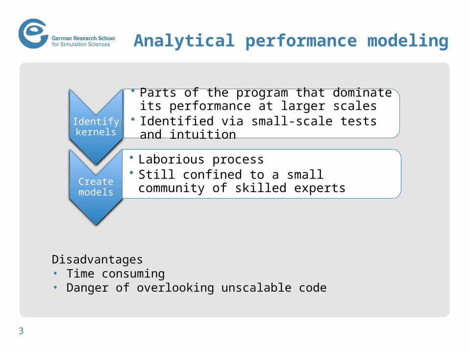
Analytical performance modeling

Disadvantages• Time consuming• Danger of overlooking unscalable code

Identify

kernels

• Parts of the program that dominate its performance at larger scales

• Identified via small-scale tests and intuition

Create

models

• Laborious process • Still confined to a small community of skilled

experts

4

Our approach

Generate an empirical model for each part of the program automatically• Run a manageable number of small-scale performance experiments• Launch our tool• Compare extrapolated performance to expectations

Key ideas• Exploit that space of function classes underlying such model is small

enough to be searched by a computer program• Abandon model accuracy as the primary success metric and rather

focus on the binary notion of scalability bugs• Create requirements models alongside execution-time models

5

Usage model

Input• Set of performance

measurements (profiles) on different processor counts {p1, …, pmax} w/ weak scaling

• Individual measurement broken down by program region (call path)

Output• List of program regions

(kernels) ranked by their predicted execution time at target scale pt > pmax

• Or ranked by growth function (pt ∞)

• Not 100% accurate but good enough to draw attention to right kernels• False negatives when phenomenon at scale is not captured in data• False positives possible but unlikely

• Can also model parameters other than p

6

Workflow

Performance measurements

Performance profiles

Model generation

Scalingmodels

Performance extrapolation

Ranking of kernels

Statistical quality control

Model generation

Accuracy saturated?

Model refinement

Scalingmodels

Yes

NoKernel

refinement

7

Model generation

Performance Model Normal Form (PMNF)

• Not exhaustive but works in most practical scenarios• An assignment of n, ik and jk is called model hypothesis• ik and jk are chosen from sets I,J Q• n, |I|, |J| don’t have to be arbitrarily large to achieve good fit

Instead of deriving model through reasoning, make reasonable choices for n, I, J and try all assignment options one by one• Select winner through cross-validation

8

Search space parameters used in our evaluation

9

Model refinement

• Start with coarse approximation• Refine to the point of statistical

shrinkage Protection against over-fitting

Hypothesis generation; hypothesis size n

Scaling model

Input data

Hypothesis evaluation via cross-validation

Computation of for best hypothesis

No

Yes

10

Requirements modeling

Program

Computation Communication

FLOPS Load Store P2P Collective…

Time

Disagreement may be indicative of wait states

11

Sweep3D

Solves neutron transport problem• 3D domain mapped onto 2D

process grid• Parallelism achieved through

pipelined wave-front process

LogGP model for communication developed by Hoisie et al.

12

Sweep3D (2)

KernelRuntime[%]

pt=262k

Increaset(p=262k)

t(p=64)

Model [s]t = f(p)pi ≤ 8k

Predictive error [%]pt=262k

sweep->MPI_Recv 65.35 16.54 4.03√p 5.10

sweep 20.87 0.23 582.19 0.01

global_int_sum-> MPI_Allreduce

12.89 18.68 1.06√p+0.03√p*log(p)

13.60

sweep->MPI_Send 0.40 0.23 11.49+0.09√p*log(p) 15.40

source 0.25 0.04 6.86+9.13*10-5log(p) 0.01

#bytes = const.#msg = const.

13

Sweep3D (3)

14

HOMME

Core of the Community Atmospheric Model (CAM)• Spectral element dynamical core

on a cubed sphere grid

KernelModel [s]

t = f(p)pi≤15k

Predictive error [%]

pt = 130k

Box_rearrange->MPI_Reduce 0.03 + 2.510-6p3/2 + 1.210-12p3 57.0

Vlaplace_sphere_vk 49.5 99.3

…

Compute_and_apply_rhs 48.7 1.7

15

HOMME

Core of the Community Atmospheric Model (CAM)• Spectral element dynamical core

on a cubed sphere grid

KernelModel [s]

t = f(p)pi≤43k

Predictive error [%]

pt = 130k

Box_rearrange->MPI_Reduce 3.610-6p3/2 + 7.210-13p3 30.3

Vlaplace_sphere_vk 24.4 + 2.310-7p2 4.3

…

Compute_and_apply_rhs 49.1 0.8

16

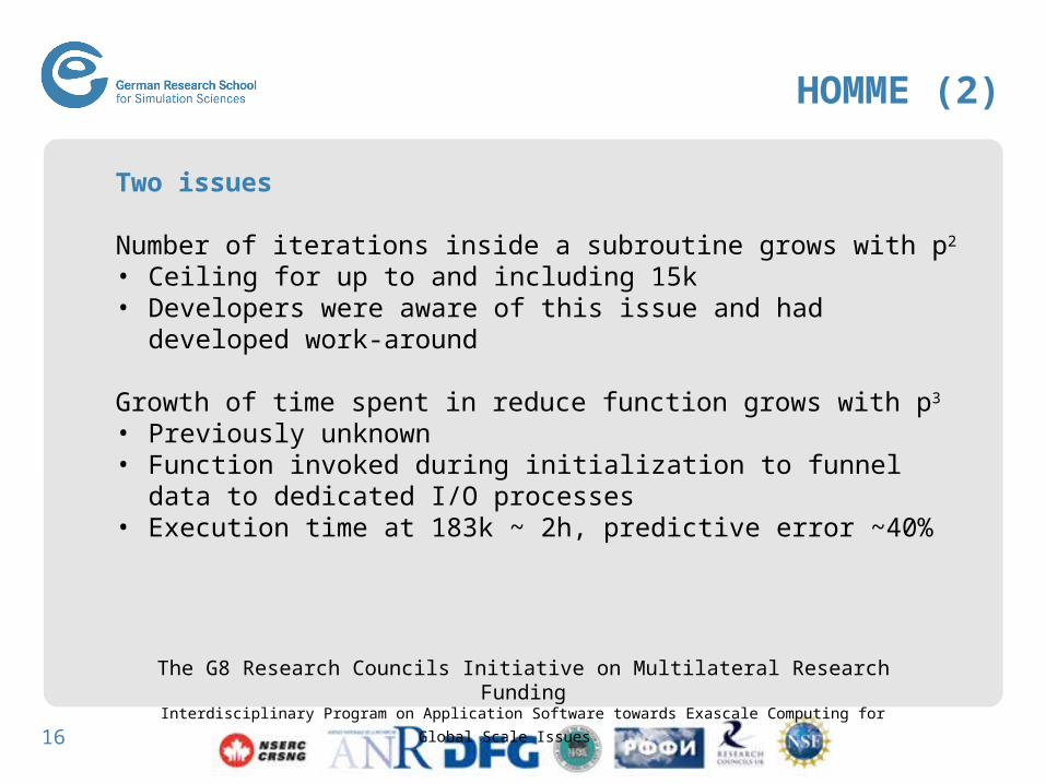
HOMME (2)

Two issues

Number of iterations inside a subroutine grows with p2

• Ceiling for up to and including 15k• Developers were aware of this issue and had developed work-around

Growth of time spent in reduce function grows with p3

• Previously unknown• Function invoked during initialization to funnel data to dedicated I/O

processes• Execution time at 183k ~ 2h, predictive error ~40%

The G8 Research Councils Initiative on Multilateral Research FundingInterdisciplinary Program on Application Software towards Exascale Computing for Global Scale Issues

17

Cost of first prediction

Assumptions• Input experiments at scales {20, 21, 22, …, 2m} • Target scale at 2m+k

• Application scales perfectly

Jitter may require more experiments per input scale, but to be conclusive experiments at the target scale would have to be repeated as well

k Full scale [%] Input [%]

1 100 <100

2 100 <50

3 100 <25

4 100 <12.5

2nd prediction comes for free

18

HOMME (3)

19

Conclusion

Automated performance modeling is feasible

Generated models accurate enough to identify scalability bugs or show their absence with high probability

Advantages of mass production also performance models• Approximate models are acceptable as long as the effort to create them

is low and they do not mislead the user• Code coverage is as important as model accuracy

Future work• Study influence of further hardware parameters• More efficient traversal of search space (allows more model

parameters)• Integration into Scalasca

20

Acknowledgement

• Alexandru Calotoiu, German Research School for Simulation Sciences

• Torsten Höfler, ETH Zurich

• Marius Poke, German Research School for Simulation Sciences

Paper

Alexandru Calotoiu, Torsten Hoefler, Marius Poke, Felix Wolf: Using Automated Performance Modeling to Find Scalability Bugs in Complex Codes. Supercomputing (SC13).