2

 

Using and developing place typologies for policy purposes

Ruth Lupton, London School of Economics and Political Science Rebecca Tunstall, London School of Economics and Political Science

Alex Fenton, University of Cambridge Rich Harris, University of Bristol

3

© Crown Copyright, 2011 You may re-use this information (not including logos) free of charge in any format or medium, under the terms of the Open Government Licence. To view this licence, visit www.nationalarchives.gov.uk/doc/open-government-licence/ or write to the Information Policy Team, The National Archives, Kew, London, TW9 4DU, or email: psi@nationalarchives.gsi.gov.uk This publication is also available on our website: www.communities.gov.uk If you require this publication in an alternative format please email: alternativeformats@communities.gsi.gov.uk Any enquiries regarding this publication should be sent to us at: Department for Communities and Local Government Eland House Bressenden Place London SW1E 5DU Tel: 030 3444 0000 February 2011 ISBN: 978-1-4098-2786-3

This report was commissioned by the previous government and is not necessarily a reflection of the current government's policies and priorities. DCLG is publishing the report in the interests of transparency. www.communities.gov.uk/archived/general-content/corporate/researcharchive/

4

Contents

Introduction .................................................................................................................5

Section 1 Place typologies: Uses and limitations .................................................10

Section 2 Key issues and decisions in the use and development of place typologies ..................................................................................................................21

Section 3 Worked example 1: Classification of neighbourhood employment deprivation.................................................................................................................39

Section 4 Worked example 2: Identifying local authorities with similar contexts to aid performance comparison...............................................................................62

Annex A: Brief descriptions of some well-used typologies ..................................77

Annex B: Useful links ...............................................................................................84

Annex C: Technical details of development of the typology of workless neighbourhoods........................................................................................................86

Annex D: Technical details of development of the nearest neighbour model for local authority performance ...................................................................................105

5

Introduction Why we use place typologies Understanding how socio-economic conditions and the performance of public sector organisations vary from one place to another is a routine and familiar element of contemporary public policy and debate. How and why are health and education outcomes, for example, so different from one place to another? To what extent are these differences a function of the performance of local authorities, schools or health providers? Which places are suffering most as a result of recession, and in what ways? Which need particular kinds of interventions? When and where does policy have to be tailored to suit specific local circumstances?

Dealing with these questions requires the capacity to identify groups of places that are similar to one another, to make sense of an almost endlessly complex picture. Ultimately, every place will have a unique combination of characteristics, but analysts need to be able to distil these in some way that makes similarities and differences apparent. Policy cannot be built on bespoke solutions for every individual place.

Many tools and techniques exist for classifying or ‘typologising’ places. Geography is often the starting point – to what extent do variations exist between north and south, or between local authority areas within a region? Simple East/West and Inner/Outer categorisations go a long way to highlighting social and economic differences within London, for example.

However, we also often need to work across geographies, identifying places which have similar conditions and outcomes although they are not geographically proximate. Tools include:

• Simple univariate rankings or indices, which simply put places in order on a single variable, or normalise a single variable to create an index (say from 0 to 100). Cut offs or quantile groups are then used to create pseudo-types. For example ‘all areas with more than 50% social housing’, or ‘all areas in the top 20% of the index’.

• Multivariate indices, such as the Indices of Multiple Deprivation, which combine different variables, sometimes using weights to give some factors greater importance than others. Again these use quantile groups or cut offs defined by natural breaks in the data to identify groups of places that are similar or different to one another.

• Classifications. Rather than cutting a ranked list into segments, these aim to identify ‘types’ of areas which have similar clusters of characteristics and which are different from other areas. For example, places might be defined as ‘retirement areas’ with a combination of a high proportion of senior citizens and housing owned outright whereas others (often in inner cities) might have distinctive clusters of rented housing, high population turnover and young and

6

minority ethnic residents. ACORN, MOSAIC, and the Office for National Statistics Output Area Classification are well known examples of these.

• Nearest neighbour models, which use similar methods but aim to identify the most similar places to any selected place, rather than to produce typologies of all places.

Box 1: Place typologies – a summary

Univariate indices or rankings Put all places in order on a single characteristic (variable), sometimes through creating an index, then cut the list at different points to define groups

Multivariate indices or rankings

Combine variables, sometimes with weightings, to make a single score, then cut the list at different points to define groups

Classifications Identify types (classes) of places which have distinct combinations of characteristics

Nearest neighbour models For any given place, identify which other places share its characteristics

Annex A provides brief information and references to some of the tools which are most commonly used.

Policy applications

The Department for Communities and Local Government (DCLG) and its predecessor departments have actively promoted the use of such classifications for nearly 30 years, since the development of the Index of Local Conditions (later the Index of Local Deprivation and Index of Multiple Deprivation) in 1981. The department has made active use of these indices in targeting interventions, such as its Neighbourhood Renewal Fund, and in evaluating performance and progress, for example in comparing the performance of New Deal for Communities areas with other areas of similar deprivation. The department has also taken the lead in the development of much better data about small areas, following the report of the Social Exclusion Unit’s Policy Action Team 18 (Social Exclusion Unit, 2000) which identified the need for a robust and wide-ranging set of indicators at neighbourhood level and gave rise to Neighbourhood Statistics.

Partly because of this work and partly because of parallel developments in the use of geo-demographic tools in the private sector and in spatial analysis software, the use of place typologies, typologies and indices is much more common that it was. Across government, these tools are used to help understand:

7

• underlying trends and policy problems, including what is driving area changes and diverging area fortunes, and whether the characteristics of areas themselves make a difference to individual outcomes (does it matter where you live?)

• which kinds of areas need priority intervention, and which can survive with reduced intervention in a time of public spending restraint

• whether different policy responses are needed in different kinds of areas – and how many varieties are needed.

• the different delivery challenges faced in different places

• the different functions that different places play in urban systems or hierarchies of settlements

• how performance can be accurately compared, taking into account relevant contextual factors and functions.

Challenges in the use of place typologies Although there is considerable enthusiasm for place typologies and widespread use, applying these tools in policy is not straightforward. Different kinds of tools, and different levels of methodological sophistication, will be appropriate in different circumstances. In some cases there will be an appropriate existing classification, while in others it may be necessary to develop something bespoke to the particular policy purpose. Departments and governmental organisations will vary in their capacity to buy existing commercial classifications, evaluate freely available tools, or develop their own.

We developed this toolkit after interviewing approximately 20 analysts and policy users across government, within DCLG and other departments including HM Treasury, the Department for Work and Pensions, the Department for Business, Innovation and Skills, the Home Office, the Department for Transport, the Cabinet Office Social Exclusion Task Force and the Welsh Assembly Government, about their use of (and views on) existing classifications and their experience developing and using their own classifications.

We also carried out a website review of work undertaken by regional observatories and regional development agencies and conducted follow-up telephone interviews to explore some of the work in more detail. In addition, we consulted a similar number of senior academics (whom we contacted through DCLG’s expert panels and through personal networks). All of these people conduct research on of area and neighbourhood characteristics and dynamics. Most had either used existing typologies or developed their own. We spoke to the key personnel involved in developing some of the publicly available and most widely used classifications.

8

The consultation raised a number of theoretical and practical questions:

• Why use classifications?

• What are their uses and limitations, methodologically and for different policy purposes?

• How to choose between different kinds of tools (such as classifications, indices and nearest neighbour models) and between different methods.

• How to evaluate existing classifications and decide whether they are fit for particular purposes.

• When, why and how to create bespoke classifications for particular purposes.

This toolkit is designed to help answer these questions, drawing on our own knowledge and the existing academic literature, the examples and insights generated by the consultation, and some new empirical work to develop and test classifications and evaluate their usefulness for policy. It is aimed primarily at policy analysts within central government departments but may also be of use to analysts in regional and local government, and government agencies, as well as to policy makers themselves who need to interpret analysis based on classifications.

Structure of the toolkit Sections 1 and 2 deal with broad questions of theory, methodology and practice.

Section 1 provides a basic introduction to place typologies, and discussion on their value and limitations for policy purposes. It gives examples of bespoke classifications that have been recently developed by analysts in central and regional government.

Section 2 explores some of the key issues in more detail. It explores the rationales for using different kinds of classifications, and provides an overview of methods. These sections are based on interviews with policy users and typology developers, and on the existing academic literature in the field. It is designed to guide potential users in their choice of approach, including when it might be necessary to develop a new classification.

Sections 3 and 4 are worked examples designed to illustrate how a department might go about developing new typologies for particular purposes, and testing their robustness. These are based on new empirical work carried out in early 2010. DCLG policy users identified two areas in which new classifications were thought to be useful. We then developed and tested typologies to address the issues identified. These sections set out the rationales for the new classifications, the methods adopted, and the result, along with an assessment of their robustness and value. It is important to stress that these examples are not designed to provide answers to the policy problems raised, nor to provide definitive tools for tackling them. DCLG may well want to adapt or develop the typologies. They are designed to give transparent demonstrations of the issues and challenges of typology uses, and insight into potential policy implications.

9

Section 3 is an example of a typology at the neighbourhood level, to identify disadvantaged areas with similar and different kinds of problems with worklessness. Section 4 is an example of a nearest neighbour tool at the local authority level, in order to identify similar authorities for the purpose of comparing performance on national indicators.

The Annexes provide further detail on:

• Some familiar and well-used existing typologies (Annex A).

• Useful links to further information (Annex B).

• The methodologies and workings involved in developing the two worked examples (Annexes C and D).

Acknowledgements

In developing the toolkit, we consulted a wide range of people who have developed classifications or who use them in their work: academics, policy experts outside government, and policy leads and analysts across government. We were supported by an advisory group. To protect against attributing views and comments to individuals, we have not named them, but we are very grateful to them for giving their time and sharing their expertise and examples of their work.

10

SECTION 1

Place typologies: Uses and limitations  

Introduction Classifications are ways of grouping places that are similar to each other and different from other places. For example, which urban settlements have similar types of functions, such as regional economic centres or dormitory towns? Which disadvantaged neighbourhoods have similar characteristics and trends to each other? In this context, classifications can be used to group any kinds of places at the sub-national level, typically local authority districts, settlements, and smaller geographies approximating to neighbourhoods such as wards, lower level super output areas or postcode sectors. Clearly there is also scope for classifications of countries or for cross-national classifications (such as of regions in Europe) but we do not deal with this here.

Most people reading this toolkit will be familiar with some commonly used UK classifications. We provide details of some these in Annex A and also in the pages which follow. Box 2 provides a simple list of some of the most familiar classifications. Most of these have been developed by government or governmental organisations and are available free of charge. Their methods and the data used are also publicly available and transparent. Some have been developed by commercial organisations and can be purchased. The methods and data for these classifications are not fully transparent, for commercial reasons.

Box 2: Some familiar classifications in the UK Local Authority Districts

• Office for National Statistics (or previously Office of Population Censuses and Surveys) classifications of local authority districts

• CIPFA (Chartered Institute of Public Finance and Accounting) – Nearest neighbour model for benchmarking local authority performance

‘Neighbourhoods’ • Office for National Statistics/Office of Population Censuses and Surveys

classifications of wards

• ACORN*

• MOSAIC*

• Office for National Statistics Output Area Classification

• Indices of Multiple Deprivation

Note: * denotes commercially developed classification.

11

Why use typologies? Typologies of places have been used for many years by geographers and sociologists, most famously to understand the functions of neighbourhoods with urban systems. For example, Park, Burgess and McKenzie (1925)1 conceptualised cities as concentric rings which served different functions, including central business districts, transition zones and suburbs. More recently (since the late 1970s), geodemographic classifications, based on the composition of resident populations, have been developed to aid understanding of likely demand for products and services.2

Place typologies have the same value in social science and policy as classifications of people into social categories. They bring some simplicity and patterning to what could be an almost endlessly complex picture of variations, and enable a shared understanding and language. For example, Park et al.’s model identified ‘transition zones’ which served as first port of call for newcomers who subsequently moved on and up as they became better off, to be replaced by new waves of immigrants. ‘Transition zones’, it might be argued, are necessary in dynamic cities and may also always be poor, despite regeneration efforts, because of their function. They might require particular kinds of public policy intervention, such as regulation of rented housing markets. The identification of this category of transition place enables a common understanding between policy makers in different cities and central government of the kind of issues at stake.

At the same time, classifications introduce greater complexity than can be derived simply from geographical distinctions. Tobler’s so-called first law of geography that “everything is related to everything else, but near things are more related than distant things”3 is not necessarily true (although it can be in many circumstances, for example broad regional differences often do pertain). Nor is geography always enough to inform some of the questions with which social policy makers are concerned. For example, it may well be true that towns that are close to the sea are more similar to each other than they are to towns which are far from the sea, and that seaside towns in the same regions may also share characteristics.

However, there are other relevant particularities that might be important to know in relation to policy: the size of the settlement, the structure and performance of industries and the history of inward investment to replace declining industry; patterns of immigration; housing policies and demand; and institutional relationships. The development of typologies based on multiple factors takes account of far more complexity in its analysis than simpler categorisations (e.g. disadvantaged or not, seaside or not, North East or not), while producing an end product – the types of areas – which is relatively simple.

                                                       1 Park, R.E., Burgess, E. and McKenzie, R. (1925). The City. Chicago: University of Chicago Press. 2 Harris, R., Sleight, P. and Webber, R. (2005) Geodemographics: neighbourhood targeting and GIS. Chichester: Wiley 3 Tobler W. (1970) A computer movie simulating urban growth in the Detroit region. Economic Geography, 46(2), pp.234-240.

12

Types of classifications Classifications, nearest neighbour models and indices

Strictly speaking, classifications produce ‘classes’ or ‘types’ or place. They are categorical tools.

Most of the typologies listed in Box 2 are accurately described as place classifications because they are primarily designed to discriminate between places, as the unit of analysis. For example, the Office for National Statistics (formerly Office of Population Censuses and Surveys) classifications of local authority districts group districts according to their function, such as ‘London suburbs’ and mining and industrial districts (places like Blackburn, Stoke-on-Trent and Barrow in Furness).

Classifications like this typically use data about the composition of the population in a place (demographic or compositional variables like age structure, household composition or ethnicity) but they may also make use of geographical variables, such as location and settlement size and economic variables. Most are, in a sense, not particularly concerned with spatial characteristics or interactions. They take pre-defined geographies, such as local authorities, wards, or output areas, and classify them according to their characteristics, rather than defining and then categorising places according to the spatial distribution of activity or the relations between places. However, there are examples of place classifications of spatial relationships. For example DCLG has identified town centres and core areas of retail activity. Boundaries and types are identified by the extent and density of the retail activity. A number of regions, in the development of their regional strategies, are examining the economic relationships between different places, and typologising places accordingly.

The availability of an increasingly wide range of data at neighbourhood level along with new, ‘geocoded’ consumer data and computational advances has also enabled the growth from the 1970s of ‘geodemographics’ – the science of identifying the probable characteristics of people based on profiles of where they live. For example, the MOSAIC classification (from Experian, see Annex A for more details) places UK consumers into 67 types and 15 groups, based on the composition of the postcodes in which they live. The focus here is on the probable characteristics of consumers, not the characteristics of places per se. However, each postcode can be ascribed a typical type based on its typical residents, such as ‘Choice Right to Buy’, ‘Brownfield Pioneers’ or ‘University Fringe’. Experian has also developed a public sector version of MOSAIC which categorises consumer needs in a similar way. Annex B provides some references for readers who are interested to know more about the development and uses of geodemographics.

Increasing interest since the late 1980s in measuring local authority performance has led to the development of another kind of classification: nearest neighbours. Such classifications identify local authorities which have similar characteristics to each other, either overall, or in relation to specific policy areas. For example, the Department for Children, Schools and Families (now the Department for Education) has developed a Nearest Neighbour Benchmarking model of local authorities to compare performance against Every Child Matters outcomes, to support the new outcome-focused inspection framework for Childrens’ Services.

13

For each authority, the model identifies others which are closest on the kinds of characteristics which predict these outcomes (variables like child poverty, social class and overcrowded housing). Comparing the performance of an authority with its neighbours provides an initial guide as to whether performance is better or worse than might be expected. The Chartered Institute of Public Finance and Accounting also has a nearest neighbours model which is designed to have broad use across a range of services.

Unlike classifications and typologies which generate groups of similar places, nearest neighbour models start with a single place and find the most similar places to it. They are particular useful for benchmarking performance and sharing good practice, but less useful as analytic tools, since groups are not generated against which to analyse other data or trends. (This issue is covered in more detail in the next section and in the worked example in Section 4.)

It should be noted that classifications and nearest neighbour models are not the only way of comparing areas. Indices are also very commonly used. The Indices of Multiple Deprivation and its component indices are probably the main mechanisms used in government at the moment to distinguish between small areas for the purposes of analysing area change, monitoring performance, setting targets and allocating funding. Often the overall index is used in analysis and policy but all the sub-domains or sub-indices which make up the set can be used for particular purposes. For example, the Department for Children, Schools and Families makes particular use of the Index of Deprivation Affecting Children Index in its analyses.

Unlike classifications, which are categorical, indices are ordinal. Rather than creating groups or types of areas on the basis of combinations of variables, indices give every area a score and rank them according to that score. Groups can be identified depending on their position on the index, such as ‘the top 10%’. However, the index itself only provides rankings, not discrete categories. This can be problematic. In an index, some places have to be at the bottom. There will always be a bottom 10% regardless of how the absolute characteristics of places change, and regardless of the fact that some of the places ranked in the bottom 10% are more similar to those ranked at 15% than those at 5%. It can be easy to see these ‘bottom places’ (or indeed ‘top places’) as discrete groups, when this is not justified by the data. Classifications provide discrete categories but they do not put them in an order.

However, this distinction can be blurred. Indices can be drawn up on single variables (univariate indices) and these can be combined to produce simple classifications. For example, ‘cumulatively advantaged’ areas might be in the bottom quartile of each of a number of indices. Similarly when indices are analysed spatially, categories may emerge, for example ‘rural pockets of deprivation’ or ‘peripheral urban deprived estates’. Furthermore, while classifications have no inherent order driven by a single variable, they are often presented in what seems like a logical order, for example with urban categories followed by rural categories, or affluent categories followed by poorer categories.

Indices can be used alongside classifications for analysis. For example, how do inner urban areas compare with rural areas on indices of access to services or health needs? Classifications can also be turned into indices by creating population

14

weighted scores for each category on in a classification. For example, we might classify responses to a survey question using a typology of places, to identify the probability of certain responses in certain types of areas. These scores could then be apportioned to all areas in the country according to their type and the size/composition of the population living in them, to make an index of places ranking highest to lowest on the survey variable. Using place typologies for policy purposes Kinds of policy use

Policy users who were consulted in the development of this toolkit identified a wide range of uses. Very few people were not making use of classifications at all or saw no value in doing so. Many consultees thought that policy uses of classifications were likely to increase, as departments sought more sophisticated evidence for policy, public funding constraints became tighter, and responsibilities were increasingly devolved to more local levels. They saw a role for central government in helping local actors to analyse the characteristics of their areas and to identify similar places in order to develop and share expertise and benchmark performance, particularly in the light of the Total Place initiative.4

Users identified two quite distinct kinds of policy use: identification of areas which needed additional or tailored support, and evaluation of performance.

The first use of classifications was to identify areas with similar and different characteristics, challenges or trends which might lead variously to:

• the need for more or less support (financial or other), which could help with understanding the efficiency of targeting towards different areas

• the need for tailored services or policy approaches, based both on objective needs and on understanding how different people might respond to different policies or messages

• being able to plan for future needs and investments.

Box 3 gives some examples of the kinds of work being undertaken.

                                                       4 www.communities.gov.uk/localgovernment/efficiencybetter/totalplace/

15

Box 3: Using classifications to understand trends and challenges

DCLG has commissioned three reports from Sheffield Hallam University to help define seaside towns and better understand their socio-economic characteristics. These are published at: www.communities.gov.uk/citiesandregions/coastaltowns/ The first report identified types of coastal town – seaside resorts (37), coastal towns and cities and estuary towns and cities. The second and third reports have provided data on, respectively, the 37 seaside towns, and on smaller seaside towns with population between 1,500 and 10,000. The latter are not in themselves typologies, although they could provide the basis for further segmentation of these settlements. Together these are being used to inform policy makers about the different challenges that face coastal areas, and how they can in different ways maximise economic prosperity while meeting social and economic challenges. The West Midlands Regional Observatory produced a classification of Lower Super Output Areas in the region that were in the top 5th of the Index of Multiple Deprivation. 67 indicators were used across many domains of social inclusion, including administrative data such as county court judgements and emergency hospital admissions, as well as Census and economic data. This identified clusters such as ‘fringe deprivation’, ‘Black Country deprivation’, ‘Black and Minority Ethnic Areas’. The aim was to identify types of areas with distinct clusters of problems that might point to different needs for support and intervention.

A number of regions, as part of the development of their regional strategies, have been developing typologies of areas depending on their economic functions, to help identify likely future trends and develop appropriate strategies for economic growth or support. For example Northern Way, supported by DCLG, the Centre for Cities and the Work Foundation, developed a typology of city relationships, based on an analysis of labour markets and business relationships identifying whether these are productive and mutually reinforcing,or where economies are relatively isolated and not benefiting from growth elsewhere. The North West Regional Information Unit has undertaken a similar study.

Yorkshire Forward for its regional spatial strategy, classified all settlements in four domains: Location (e.g. free-standing), Service (e.g. sub-regional centre or local service centre), Functions (e.g. tourism, employment centre) and Prosperity (whether prosperous, stable or less prosperous). DCLG has identified areas of town centre activities and retail cores: www.communities.gov.uk/publications/corporate/statistics/retailcores19992004

Similarly, many central, regional and local governments and agencies, as well as academics were conducting analyses that produced area comparisons or indices, although not necessarily developing into full blown classifications. For example, Midgley et al (2003)5 identified ‘bundles’ of challenges: access to employment, quality of employment, low earnings, access to housing, housing conditions and

                                                       5 Midgley, J., Hodge, I. and Monk, S. (2003) Patterns and Concentrations of Disadvantage in England: A rural-urban perspective. Urban Studies, 40(8), pp.1427-1454.

 

16

examined the prevalence of these in wards in urban and rural areas using the Office for National Statistics ward classification. This could be taken further to re-classify wards e.g. urban wards with poor housing. West Midlands Regional Observatory has conducted analysis to determine which areas are vulnerable to recession in the short, medium and longer term. Variables indicating vulnerability in each time period have been combined (each with the same value) into an index. Cut offs of the index can be used to identify areas of highest vulnerability.

Some departments were undertaking or considering complex analyses to identify areas that had certain compositional characteristics (for example people in demographic types who might be most likely to respond to policy change) or combinations of population composition and area characteristics (for example areas with many older residents and poorly insulated housing).

Section 3 of the toolkit provides a worked example of the development of a classification to support better understanding of the challenges face in different areas – differentiating areas with different kinds of worklessness.

Our consultation with policy users and academics revealed both enthusiasm for more complex analyses and scepticism. Greater understanding (especially of behaviour) leading to fine-tuning of policies was seen to be valuable both in increasing the impact of policies which had previously been targeted in a more broad-brush fashion, and in ensuring the money was spent wisely in a time of restraint. However, there were also those who were argued that such developments were ideologically unwelcome because they contributed to the search for individuals who were ‘outside the mainstream’ or ‘hard to reach’ rather than looking at structural reasons for disadvantage and inequality. Some users felt that complexity of analysis and targeting could mask more important political and ideological concerns about the distribution of resources. These debates go beyond the scope of this toolkit but are nevertheless worth noting. The existence of the tools to produce fine-grained analysis based on compositional traits does not necessarily mean they should always be used to guide policy.

A second policy use was the evaluation of performance. Policy colleagues wanted to know which areas could reasonably be compared with one another. To what extent did areas manifest distinct groupings of characteristics that created different challenges for delivery? Section 4 of the toolkit provides a worked example of a classification for this purpose.

Limitations and responsible uses

Many users pointed out that there are limitations to the use of classifications (geodemographic and otherwise) in policy and that they need to be used thoughtfully and appropriately. It was generally agreed that typologies should be used descriptively rather than predictively. In other words, they can tell us what types of place are similar to one another, as a basis for other analysis that unpacks why that is the case, what might happen in the future, or what kind of policy intervention might work. Users should not seek to use typologies, on their own, to explain or predict. It was also agreed that typologies should generally not be used on their own as tools for targeting policy or resources. Rather they should be used to enhance understanding and to guide

17

development of a spectrum of policies that could be variously appropriate in different places. In the same vein, some analysts argued that while classifications are attractive because they bring simplification and a shared language, there is a danger that this leads to too much simplicity, the sense that all one needs to know about a place is the category it falls into. They argued that classifications should be a starting point for more complex analyses rather than taking their place. Knowing what types of places there are and what kinds of different mechanisms are prevalent in each is what is ultimately useful, rather than a final answer that x place is of x type. This is particularly the case because, ultimately, the number of types in a classification is determined by the developer. There is a trade-off between having a small number of types, which is easy to grasp and remember, but where each of the types may have a good deal of internal variety, and having a larger number, which is more accurate but may introduce too much complexity and put potential users off. Clearly ‘x’ place might be defined one way in a five group typology, but another way in a ten group typology. Classification is not an exact science. One way to deal with this is the hierarchical approach adopted in the Output Area Classification and a number of other classifications, where subgroups are nested within groups, which are nested within super-groups. This enables policy users to work with high-level categories, but supported by more detailed analysis of patterns within them. A particularly important point was that, while classifications can be helpful in guiding funding priorities, it is problematic to use them for funding allocation. Any mechanism used for funding allocation needs to be defensible to legal challenge. Some analysts pointed out that classifications may be most appropriately used to identify the kinds of areas that should be eligible for funding, but another mechanism should be used actually to allocate money. For example, funding could be allocated on the basis of more local needs assessments or on the strength of local authority plans. In any case, targeting using typologies is inevitably imperfect.6 Both analysts and policy users felt some degree of nervousness about using existing classifications, because they were not always sure of the basis on which types were developed. Many government departments had bought licenses to use commercial classifications (particularly MOSAIC) but were particularly nervous about these because, for commercial reasons, the underlying variables are not fully known nor is it clear what exact methodology has been used. Knowledge of the relatively recent Office for National Statistics Output Area Classification was patchy – some people knew about it and were using it, while others were not. It was noted that the Output Area Classification had not been actively marketed to users, unlike the commercial classifications. Many potential users were aware of the existence of these tools (Output Area Classification and commercial classifications) and some had purchased them, thinking they would be valuable, but had not had the time to develop full confidence in their use. The number of confident users we encountered was relatively small.                                                        6 Tunstall, R. and Lupton, R. (2003) Is targeting deprived areas an effective means to reach poor people? An assessment of one rationale for area-based programmes. CASEpaper70. London: CASE. http://sticerd.lse.ac.uk/dps/case/cp/CASEpaper70.pdf

18

In discussion of the relative advantages of these alternatives for small area classification (commercial vs Output Area Classification), analysts tended to see the advantage of the Output Area Classification as being free and transparent in its methodology and document, and the advantage of commercial classifications as being better known and using more up-to-date data (the Output Area Classification is entirely Census-based). Commercial classifications use a combination of Census and more recent variables, including those garnered from marketing databases about consumer behaviour. This more recent picture was intuitively attractive to users, although in the absence of a transparent methodology it is not possible to assess which variables are driving the typology and what difference these make. An additional advantage of the Output Area Classification, although not one that was specifically raised in our consultation, is that it includes information on the uncertainty with which an output area has been allocated to a given class because it includes the distances to each of the category centroids.7 For local policy use, this could be particularly valuable, and would encourage the use of other data alongside the Output Area Classification to understand characteristics of areas that appeared in odd categories. On the other hand, commercial products offer the potential to aggregate postcodes to Output Areas in order to see the mix of categories within Output Areas – a facility not available with the Output Area Classification. Almost no-one we consulted was confident of being able to determine which of the classifications on the market provided the greatest discriminatory power or was most predictive of the outcomes they wanted to look at. Statistical techniques are available to do this8,9, although they are not widely used. Some consultees emphasised that the statistical robustness of the typology relative to others was not the only criterion for choosing it. Transparency and making sense to end users was also important. The cost of statistical analysis and testing of typologies was not always justified by the additional benefits gained. Both analysts and policy users were in agreement that while it was not necessary for policy clients to be able to perform analysis using classifications, they did need to be able to trust the results. It was agreed that analysts should take responsibility for clear guidance to policy users on how classifications had been developed and the information they could and could not provide. In particular, users need to be clear when data is modelled or real, what the data source is, how old the data is, and when it relies on very small numbers of cases. Transparent robustness tests were also thought to be valuable, including statistical tests such as testing for the effect of removing one or more variables, and non-statistical tests such as ‘road-testing’ the classifications with people working in the field. This toolkit, including the Annexes on particular classifications, is designed to provide support in this.

                                                       7 This dataset is available at www.sasi.group.shef.ac.uk/area_classification/index.html under the heading ‘Fuzzy Classification’. 8 Benton, T., Chamberlain, T., Wilson, R. and Teeman, D. (2007).The Development of the Children’s Services Statistical Neighbour Benchmarking Model: final report. Slough: NFER. 9 Ojo, A. (2009) A Proposed Quantitative Comparative Analysis for Geodemographic Classifications. Published online by the Yorkshire and Humber Public Health Observatory. www.yhpho.org.uk/resource/item.aspx?RID=10170 

19

Names of categories such as ‘mining town’ or ‘multicultural inner city’, are particularly valuable to policy users (and indeed the current lack of names at lower levels of the Output Area Classification was seen as a drawback), but it was also recognised that names may be stigmatising and misleading. The choice of name can induce people to infer more about an area than is justified by the underlying data, so that the typology takes on more (and misleading) meaning than the analysis suggests. In particular, care must be taken to avoid stereotypes and prejudice. Simple explanations of the categories, produced by analysts, can help to add depth and understanding. Some respondents also recommended that substantial time is taken at the naming stage in the development of a typology, to consult with users about what they take names to mean, and to demonstrate the extent to which these are supported by the analysis.

A final issue arising from the consultation we conducted with analysts and users was concern about the use of national classifications for local and regional analysis. Users in regional government, and some academics, tended to argue that national classifications may not give the granularity needed for local analysis. A particular concern was that the distinctive characteristics of London tend to drive the emergence of types in classifications that are England, Great Britain or UK wide. Important differences between places that are not in London may be lost.10 Policy users interested particularly in rural areas and small settlements also find that classifications can be driven by the characteristics of the more numerous urban areas. People working in specific regions argued that classifications may need to be devised at local level or supplemented by locally available data. Local analysts are best placed to do this, but there is no need to reinvent the wheel each time. Some analysts at regional level felt that they would benefit from being able to share practice and replicate existing methodologies. This toolkit goes some way to providing examples and methodological guidance. DCLG could consider other ongoing ways of publicising developments and enabling the transfer of good practice.

Summary It is clear from this introduction that place typologies take different forms, use different methodologies and have different practical applications. Our interviews with analysts and policy users showed that while some have very clear views about the benefits of different kinds of classifications for different purposes, others are less sure which is the right choice.

The next section of the toolkit is designed to help clarify and exemplify the different approaches that can be taken, by working through some of the underlying principles that underpin the choice of approach.

                                                       10 For this reason, some regions make a case for ‘regional OAC’ or similar products. ACORN has developed separate classifications for metropolitan areas and also for Scotland and Ireland. The need for regional classifications remains to be fully tested empirically.

20

We look at:

• whether to use standard (existing) classifications or develop new ones bespoke to particular policy issues

• the different benefits that can be gained from classifications and from nearest neighbour approaches

• whether to develop classifications starting from theory or data, and the methods that follow

• what kinds of variables might be included

• the importance of spatial coverage and units of analysis.

21

SECTION 2

Key issues and decisions in the use and development of place typologies  

Standard or bespoke classifications? A first question that faces policy analysts and users who want to categorise places for policy purposes is whether to use an existing classification or to develop (or commission) one which is designed specifically to be fit for the particular purpose at hand (such as the ones in Error! Reference source not found..

This is partly a pragmatic issue. Some of the academics and policy researchers of area and neighbourhood typologies we consulted pointed out the scale of the intellectual and practical task involved in developing bespoke typologies and warned that for some purposes, the gain in understanding achieved might not be worth the effort. Some felt that existing typologies had much to offer in pragmatic terms, being accessible, well-known, and apparently revealing. They emphasised that the primary value of typologies is to provide a way of simplifying complex patterns as a way into more complex analysis (of cause and effect, for example) or work with people at local level. They should not be seen as performing the analysis in themselves. For this reason, existing tools may do the job.

Departments wanting to develop new typologies need in-house capacity, and/ or funding for commissioning. Some central government departments and regional observatories do contain staff with extensive expertise in these issues, including in some cases PhDs in spatial analysis. However, many others do not. We found little evidence at central government level of sharing of expertise and examples between departments, although there was enthusiasm for this and positive feedback on the work of DCLG’s Spatial Analysis Unit and its potential roles in providing guidance and support. Some researchers pointed out that commercial suppliers can provide help with practicalities and analysis for organisations that do not have the staff time or expertise themselves. In other words, departments using such classifications are buying more than the classification itself.

However, this is not just a pragmatic issue. There are different logics for the different approaches which we set out below.

Standard classifications

One view is that classifications should identify places that are clearly distinguishable from each other on a set of core geographic and demographic characteristics that typically remain fairly stable over time, and which ‘make sense’. For example, we might make a distinction between inner urban estates and middle class suburbs. Such categories should then become familiar and provide a shared language and a common basis for analysis of other characteristics, outcomes, attitudes, trends and

22

perhaps service performance. They could provide a consistent basis for many analyses, so that a comprehensive understanding is built up about different types of places. Of course, it is likely that categories will change over time, and indeed they must if they are adequately to reflect social and economic change, but changes would be expected to take place over relatively long time scales (perhaps 10 years).

Box 4: Example of a standard classification – The Office for National Statistics/Office of Population Censuses Surveys classification of local authority districts

The Office of Population Censuses and Surveys district classification was first produced in the1970s based on cluster analysis of 1971 Census variables. This was repeated in 1981 and 1991, and again in 1996 to take account of local government reorganisation. The same approach is used to produce classifications at smaller geographies (such as wards and health areas), forming a loose system of classifications. The 2001 version (from the Office for National Statistics) is based on cluster analysis of 42 census characteristics covering demographic structure, household composition, housing, socioeconomic characteristics, employment and industry sector. The structure produces a three tier classification of local authority families, groups and clusters although only families and groups have names. The families (in bold)and groups in the 2001 version are as follows:

- Cities and Services o Regional centres o Centres with Industry o Thriving London periphery

- London Suburbs - London Centre - London Cosmopolitan - Prospering UK

o Prospering Smaller Towns o New and Growing Towns o Prospering Southern England

- Coastal and Countryside - Mining and Manufacturing

o Industrial hinterlands o Manufacturing Towns

The categories in the classification do change each time it is produced, to take account of changes in the underlying variables. For example, the emergence in the 2001 version of three London categories (as well as ‘thriving London periphery’ reflects London’s recent growth and diversity. However, the categories largely reflect locational factors and long-term economic structures, and thus provide a solid basis for analysis of outcomes and trends. Earlier versions have been widely used, for example in the State of the English Cities report (2000), in analysis of population and social class change, migration and gentrification, and patterns of labour supply

23

and demand).11

Standard classifications need to include all places at the relevant spatial scale, since they will be used for many different purposes, thus they are likely to have numerous categories, some of which will be redundant for some users. For example, analysts of rural issues will not be interested in urban places, and vice versa. This has implications which we discuss later under the heading ‘Coverage and Scale’. They are also designed for longevity, so are unlikely to be based on volatile indicators, or on recent trend data. They tend to include one spatial scale only (for example they are a classification of districts or neighbourhoods).

Bespoke classifications

Amongst the academic users of area and neighbourhood typologies we consulted, most preferred to develop their own typologies, or to adapt existing ones, bespoke for their particular enquiries, rather than using pre-existing typologies. This was principally because they wanted typologies that fitted their research questions more closely than ones designed for multiple purposes. The typologies often formed the basis for further quantitative or qualitative analysis, so had to be seen to be coherently related to the core questions of the research, rather than ‘picked off a shelf’. Many policy analysts and users also preferred this approach, even if they could not always find the resources to carry through and develop their own classifications. A number of rationales were given for developing bespoke classifications (Table 1).

                                                       11 Champion, A., Green, A., Owen, D., Ellin, D. and Coombes, M. (1987) Changing Places: Britain’s Demographic, Economic and Social Complexion. London: Edward Arnold. Green, A. and Owen, D. (1998) Where are the Jobless. Changing Unemployment and non-employment in cities and regions. Bristol: Policy Press. Hills, J. (1995) JRF Enquiry into Income and Wealth. Champion, T. (2004) Unpublished background paper to State of the Cities report – available on line at www.ncl.ac.uk/curds/publications/publications/staff/tony.champion).

24

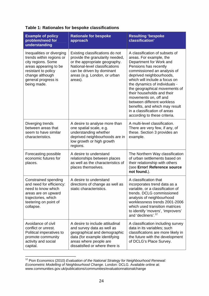
Table 1: Rationales for bespoke classifications

Example of policy problem/need for understanding

Rationale for bespoke approach

Resulting ‘bespoke classification’

Inequalities or diverging trends within regions or city regions. Some areas appearing to be resistant to policy change although general progress is being made.

Existing classifications do not provide the granularity needed, or the appropriate geography. National-level classifications can be driven by dominant areas (e.g. London, or urban areas).

A classification of subsets of areas. For example, the Department for Work and Pensions has recently commissioned an analysis of deprived neighbourhoods, which will include a focus on the dynamics of individuals - the geographical movements of their households and their movements on, off and between different workless benefits, and which may result in a classification of areas according to these criteria.

Diverging trends between areas that seem to have similar characteristics.

A desire to analyse more than one spatial scale, e.g. understanding whether deprived neighbourhoods are in low growth or high growth regions.

A multi-level classification. There are very few, if any, of these. Section 3 provides an example.

Forecasting possible economic futures for places.

A desire to understand relationships between places as well as the characteristics of places themselves.

The Northern Way classification of urban settlements based on their relationship with others (see Error! Reference source not found.).

Constrained spending and need for efficiency: need to know which areas are on upward trajectories, which teetering on point of collapse.

A desire to understand directions of change as well as static characteristics.

A classification that incorporates trend data as a variable, or a classification of trends. DCLG commissioned analysis of neighbourhood worklessness trends 2001-2006 which used transition matrices to identify ‘movers’, ‘improvers’ and ‘decliners’.12

Avoidance of civil conflict or unrest. Political imperatives to promote community activity and social capital.

A desire to include attitudinal and survey data as well as geographical and demographic data (for example identifying areas where people are dissatisfied or where there is

A classification including survey data in its variables; such classifications are more likely in the future with the development of DCLG’s Place Survey.

                                                       12 Pion Economics (2010) Evaluation of the National Strategy for Neighbourhood Renewal: Econometric Modelling of Neighbourhood Change. London: DCLG. Available online at: www.communities.gov.uk/publications/communities/evaluationnationalchange

25

conflict and distrust).

Any policy problem or issue.

A concern that standard classifications may have out-of-date data that makes them inaccurate. Availability of a particular specialised dataset that is not available or used in other classifications.

A classification based on up-to-date data. Commercial typologies claim to be based on up-to-date data such as data from lifestyle surveys.

Key decisions on distribution funding to be decided and announced.

A concern about the usability of an existing typology and how accessible it is to policy makers or members of the public.

A transparent classification (e.g. transparent about data or methodology or with transparent names of classes).

We summarise some of these differences between standard and bespoke classifications in Figure 1 below. Anyone thinking about developing a new classification needs to be clear why it is necessary and what it adds, relative to the costs of development and the likelihood that the analysis may have a short shelf-life. Sections 3 and 4 of this toolkit are worked examples which set out some real-life rationales for bespoke classifications, and then develop and evaluate them.

Figure 1: Purposes of standard and bespoke classifications

26

Classifications or nearest neighbour models Whether or not a new classification is to be developed, another question that needs to be answered is whether it is a classification that is needed or a nearest neighbour model. A classification will include all areas within one of a number of classes or groups. A nearest neighbour model starts from the perspective of a single place and identifies the other places nearest to it. In part, this is a question about usage. Individual local authorities tend mainly to be interested in their own comparators rather than the overall picture, and this may also be the case for those in inspectorate and performance monitoring purposes.

However, this is again not just a pragmatic issue. The results produced will differ in important ways, generating different groups that have more or less reciprocity, are similar or different in size and where it more or less clear what degree of similarity there is between members of the same group (see Table 2 and the example in Section 4 for a fuller coverage of these issues). We show this by way of an example.

Figure 2 shows eight local authorities plotted on two axes of variables that might be thought to impact on educational attainment: the deprivation score for the local authority and the proportion of pupils speaking English as an Additional Language. Local authority A could be regarded as facing the fewest challenges, with low deprivation and low English as an Additional Language, while local authority D, with high deprivation and moderately high English as an Additional Language might be said to face the most challenges.

If we were to go about grouping these authorities for comparison purposes using cluster analysis, we would probably find that initial results produce a group of three relatively advantaged authorities (A, B and G), a group of four relatively disadvantaged authorities (C, D, E and H) and a group of one outlier (F). A characteristic of classification based on cluster analysis is that they will throw up the best fitted groups for any selected number of classes or groups. These groups will not necessarily be the same size.

Very small groups may be suitable for comparison purposes but the single outlier in this example is unsatisfactory because it has no-one to be compared with. To remove this problem, we might choose to reclassify in order to produce just two groups that are, overall, more similar to each other than to those in the other group (Figure 5). In this case, the outlier, F, joins the low deprivation group. Note that with the classification approach, relationships are reciprocal. E is in D’s group and D is in E’s group, and so on.

27

Figure 2: A classification (groups) approach to comparison

This result might be seen to be rather unfair for comparing performance. Although in the high deprivation group, the authorities are all fairly close to each other and closer to each other than they are to authorities in the other group, this is not the case in the low deprivation group. Authority G in particular might argue that it is unfair to put it in a group with F, where it is really closer to E than to its own group member, F.

The nearest neighbour approach works by starting from the actual location of each authority to identify its closest comparators. We simply find those with the smallest distance.

Figure 3 illustrates what would happen in this case, to whom authorities D and G are compared with. D retains the same comparators as in the previous model: H, E and C. However, G is now compared with E, B and A, and not with F. Note that although G is compared with E, E would not be compared with G, because it is more like H, C and D than it is like G.

28

Figure 3: A nearest neighbour approach to performance comparison

29

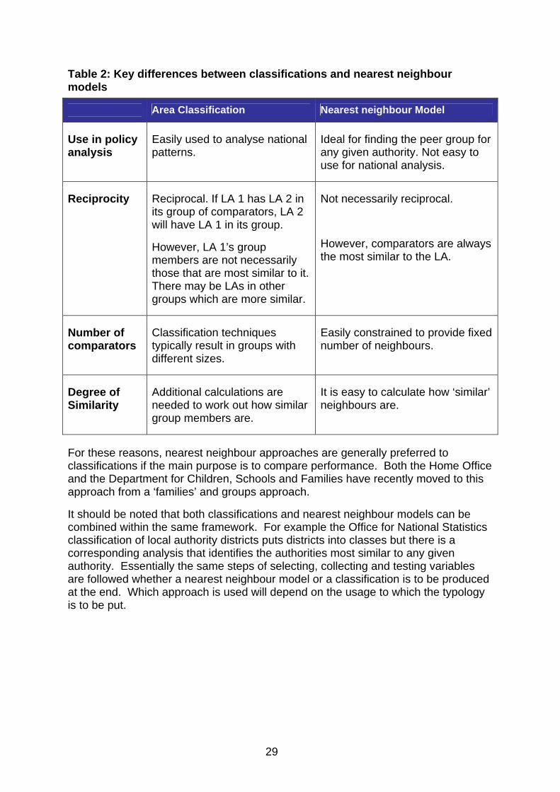
Table 2: Key differences between classifications and nearest neighbour models

Area Classification Nearest neighbour Model

Use in policy analysis

Easily used to analyse national patterns.

Ideal for finding the peer group for any given authority. Not easy to use for national analysis.

Reciprocity Reciprocal. If LA 1 has LA 2 in its group of comparators, LA 2 will have LA 1 in its group.

However, LA 1’s group members are not necessarily those that are most similar to it. There may be LAs in other groups which are more similar.

Not necessarily reciprocal.

However, comparators are always the most similar to the LA.

Number of comparators

Classification techniques typically result in groups with different sizes.

Easily constrained to provide fixed number of neighbours.

Degree of Similarity

Additional calculations are needed to work out how similar group members are.

It is easy to calculate how ‘similar’ neighbours are.

For these reasons, nearest neighbour approaches are generally preferred to classifications if the main purpose is to compare performance. Both the Home Office and the Department for Children, Schools and Families have recently moved to this approach from a ‘families’ and groups approach.

It should be noted that both classifications and nearest neighbour models can be combined within the same framework. For example the Office for National Statistics classification of local authority districts puts districts into classes but there is a corresponding analysis that identifies the authorities most similar to any given authority. Essentially the same steps of selecting, collecting and testing variables are followed whether a nearest neighbour model or a classification is to be produced at the end. Which approach is used will depend on the usage to which the typology is to be put.

30

Theory or data: What should drive a classification? All classifications depend on a combination of theory (about what makes places similar or different to each other) and analysis of data. However, some are more data-driven and some are more theory-driven. Our consultation revealed different views about these approaches.

Data-driven typologies or classifications

Data-driven classifications are developed by combining a large number of variables about areas using statistical techniques. The principal mechanism is cluster analysis to see how these factors or components group together in areas, such that some areas have one distinctive group of factors (such as terraced housing and South Asian populations) and some have another group (such as detached housing and people in professional occupations).

Typically, the correlations between available variables are checked to ensure that the classification is not based on many variables that are effectively measuring the same thing. Factor analysis or principal components analysis can also be used to distil large numbers of variables into a smaller number by identifying underlying themes and relationships.

In a data driven classification, the analyst is not attempting to shape the classification by deciding what the final groups should look like, nor making judgements about which variables are theoretically important or which should have more weight. The outcome is therefore a classification which is theory-neutral – the data is doing the talking. Such classifications arguably have broader uses than those that are seen to have been based on judgement.13

                                                       13 It is arguable that there is no such thing as a neutral classification since some decisions are always made by someone about which variables should be included. For example, Census-based classifications rely on what someone decided to put in the Census and on the decision to use the Census, and a particular spatial scale, as the data source. The theorisation, however, is designed to take a back seat in the formation of the typology.

31

Box 5: Example of a data-driven classification

The Office for National Statistics Output Area Classification 41 variables were used from the 2001 census. These covered demography, household composition, housing, socio-economic factors and employment. The variables were chosen partly on the basis of theory (e.g. gender was not included since it was considered to say little about an area) and partly because of their inter-correlation or distribution (for example variables which are very heavily skewed to one end do not work well in a classification. Consistency with the Office for National Statistics classifications for wards and local authorities was also desired. All variables were standardised across the same range to enable them to be used in the classification. A decision was made to have a three-level classification, with different levels useful for different kinds of purpose. K-means clustering was applied to identify groups which contained places most similar to each other and different from the rest. This produced 7 super-groups at the top level of the hierarchy, 21 groups, and 52 sub-groups. Each could be profiled in terms of its scores on the variables. The super-groups and groups were then given names which best described them. For example, a super-group ‘Constrained by Circumstances’ contains groups including ‘Senior Communities’, ‘Public Housing’ and ‘Older Workers’.

Theory driven typologies or classifications

Some classifications are not driven by data in this way but by theory.

In a purely theoretical classification, the analyst uses existing knowledge to identify theoretical types, and then uses data to identify which areas fall into which type. Box 6 is an example of such a classification. Typically such classifications will include a much smaller number of variables than a data-driven classification. Their advantages are that they build on a lot of existing knowledge. They make sense to policy users because it is obvious what is driving the classification, and they can be relatively quick to produce.

However, such classifications are clearly open to the question on the grounds that, had other variables been included, different results would have been found. The selection of variables reflects only one theoretical perspective, which may then be given undue weight in policy thinking. For example, one theory about neighbourhood decline is that neighbourhood fortunes are driven very largely by economic forces at city or regional levels, and by the extent to which individual neighbourhoods are connected to these wider opportunities. A classification based on this theoretical perspective would use economic variables at city or regional scales, and geographic measures of proximity. It would not include measures that could be seen as important from other theoretical perspectives, such as the history of policy interventions, the performance of local institutions or the level of community social capital or efficacy.

32

Purely theoretical classifications can be subjected to various tests in response to these questions. These include:

• ‘road-testing’ with people who work in the field and can highlight when results seem fundamentally at odds with their understandings

• ‘road-testing’ with people who are sceptical about the theoretical premises of the classification

• testing the robustness of the classification to inclusion of different variables or data collected at different time periods

• cross-checking against other existing classifications.

Box 6: Example of a theory led classification

Functional Roles of Deprived Areas DCLG recently commissioned the Centre for Urban Policy Studies at Manchester University to conduct analysis of the functional roles that different deprived areas play.14 The rationale was that different policy approaches might be relevant for different areas. For example, areas that are subject to gentrification may generate displaced households whose need for affordable housing must be met. Rather than starting with a large number of variables, the team used their existing knowledge of the functions of deprived areas to generate a four-way classification, based on patterns of in and out migration: whether people moved from and/or to more deprived, similar or more advantaged areas. For example, in some deprived areas, people move in from similarly deprived areas and move out to similarly deprived areas. These were described as Isolate areas. Census migration data were then applied for Lower Super Output areas to fit deprived areas into these groups. The robustness of the typology was tested by:

• testing the groups against the Index of Multiple Deprivation to make sure that they were not just measuring deprivation

• testing the groups against expectations, and in particular localities

• testing them against other Census variables to see if their socio-economic profiles accorded with what might be expected.

                                                       14 Robson, B., Lymperopoulou, K. and Rae, A. (2009) A typology of the functional roles of deprived neighbourhoods. London. DCLG.

 

33

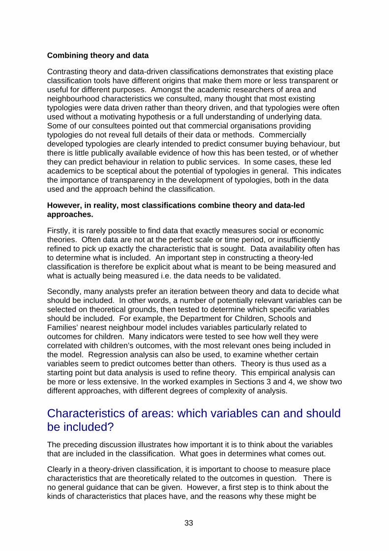
Combining theory and data

Contrasting theory and data-driven classifications demonstrates that existing place classification tools have different origins that make them more or less transparent or useful for different purposes. Amongst the academic researchers of area and neighbourhood characteristics we consulted, many thought that most existing typologies were data driven rather than theory driven, and that typologies were often used without a motivating hypothesis or a full understanding of underlying data. Some of our consultees pointed out that commercial organisations providing typologies do not reveal full details of their data or methods. Commercially developed typologies are clearly intended to predict consumer buying behaviour, but there is little publically available evidence of how this has been tested, or of whether they can predict behaviour in relation to public services. In some cases, these led academics to be sceptical about the potential of typologies in general. This indicates the importance of transparency in the development of typologies, both in the data used and the approach behind the classification.

However, in reality, most classifications combine theory and data-led approaches.

Firstly, it is rarely possible to find data that exactly measures social or economic theories. Often data are not at the perfect scale or time period, or insufficiently refined to pick up exactly the characteristic that is sought. Data availability often has to determine what is included. An important step in constructing a theory-led classification is therefore be explicit about what is meant to be being measured and what is actually being measured i.e. the data needs to be validated.

Secondly, many analysts prefer an iteration between theory and data to decide what should be included. In other words, a number of potentially relevant variables can be selected on theoretical grounds, then tested to determine which specific variables should be included. For example, the Department for Children, Schools and Families’ nearest neighbour model includes variables particularly related to outcomes for children. Many indicators were tested to see how well they were correlated with children’s outcomes, with the most relevant ones being included in the model. Regression analysis can also be used, to examine whether certain variables seem to predict outcomes better than others. Theory is thus used as a starting point but data analysis is used to refine theory. This empirical analysis can be more or less extensive. In the worked examples in Sections 3 and 4, we show two different approaches, with different degrees of complexity of analysis.

Characteristics of areas: which variables can and should be included? The preceding discussion illustrates how important it is to think about the variables that are included in the classification. What goes in determines what comes out.

Clearly in a theory-driven classification, it is important to choose to measure place characteristics that are theoretically related to the outcomes in question. There is no general guidance that can be given. However, a first step is to think about the kinds of characteristics that places have, and the reasons why these might be

34

important. Selections can then be made selections in consultation with experts in the area or with reference to specialised literature.

Lupton and Power (2002)15 suggest that it is helpful to think about places as having certain ‘intrinsic’ or hard-to-change characteristics, such as their location, economic structure, and housing stock. Some of these can be changed (they are not intrinsic in the strict sense of the word), but change is slow, and characteristics of this kind tend to be embedded over long periods.

‘Intrinsic’ characteristics are strongly linked to population composition and dynamics. Workers locate close to industry. People with low skills and earning capacity move into areas of lower quality, lower cost housing. New migrants tend to settle near ports or in major cities, from which some will disperse. In cities with growing economies, areas of low cost private housing close to city centres become gentrified. Thus to a certain extent, we may read off population composition and dynamics from intrinsic characteristics (assuming that similar places behave in similar ways), or we may want to add compositional variables in order to understand better the variation between areas with similar geographic and economic characteristics.

The combination of place and people also gives rise to ‘acquired’ characteristics which are more prone to change. These include physical/environmental characteristics, social interactive characteristics, political and institutional characteristics, or economic characteristics. Again, depending on the purpose of an area classification, we may want to read these off from geographical and demographic variables, or we may want to measure them directly.

Table 3 shows summarises this approach to thinking about place characteristics and gives some examples of measures. It is evident that each type of characteristic might be viewed as context, and therefore to be included in a classification, or as an outcome, depending on the purpose of the classification. For example a policy maker interested in understanding migration patterns might classify places by their ‘intrinsic’ characteristics and analyse the extent to which demographic characteristics were changing over time in places of different types. On the other and someone interested in understanding local authority performance or would include demographic factors in a classification, in order to identify places with different social and community contexts. Someone interested in promoting third sector activity might want to consider local authority performance or political control as a contextual variable to be included in a classification.

                                                       15 Lupton, R. and Power A. (2002) Social exclusion and neighbourhoods. In J. Hills, J. Legrand and D. Piachaud (eds). Understanding Social Exclusion. Oxford: Oxford University Press.

 

35

Table 3: Place characteristics

Type of Characteristics

Examples Why important Examples of measures

‘Intrinsic’ or hard to change characteristics of place

Geographical factors such as proximity

Economic factors such as industrial structure

Physical factors such as housing stock

Influence access to jobs and services

Distance to nearest major settlement or transport link

Census or Annual Business Enquiry measures of occupational structure

Measures of labour demand such as job density or economic productivity

Census or English Housing Survey measures of building type, age, size and quality

Population composition and dynamics

Age, gender, ethnicity, social class of residents

Migration

Influence labour supply, household structure, service needs, social networks and norms, culture and preferences

Census of Population and administrative data (such as GP registrations and annual school census)

Acquired characteristics

Norms, attitudes and behaviours

Social relations and networks

Environmental characteristics such as noise, graffiti, traffic, pollution

Institutional characteristics such as local services and resources

Political characteristics

Influence behaviour and the experiences that people have of living in places

Survey data on social networks and peer relations

Measures of environmental quality

Survey data on attitudes and concerns

Political control, local authority performance, strength of voluntary sector

36

There are also other important considerations in the choice of variables:

• Both absolute and relative variables may be relevant. The characteristics in the table above are all absolute. However, places are in some ways meaningful because of the relations between them. For example, it might be relevant to know what position a neighbourhood has in the local housing market, not just the absolute value of prices or rents.

• We might sometimes be interested in diversity within an area (for example of tenure or ethnicity) as well as an overall score.

• Historical factors, direction and speed of change may be important, as well as current factors. It is unusual to see an area classification which also explicitly incorporates a time dimension. Some of the academics we consulted argued that this brings an unnecessary level of complexity, the purpose of a classification being to identify similar places at any given point in time in order to be able to see how such places change relative to each other. However, there is no reason why long-run change prior to the time at which characteristics are measured should not in itself be regarded as a characteristic. For example, is an area declining or growing?

There can be no right answer to this, since what is relevant will vary a lot from one case to the next. The key issue is not simply to take variables that happen to be available but to develop a theory about what kinds of place factors might be important, and to seek measures of these. This process is best illustrated by worked examples in Sections 3 and 4.

Spatial coverage and units of analysis Finally there are issues of coverage and scale.

The coverage of a classification (whether England only, England and Wales, Great Britain or UK for example) may well be determined by policy considerations if a bespoke classification is being considered, or by what already exists if a pre-existing classification is being used. The choice of spatial units for the classification may also be pragmatically determined. For example, policy users involved in evaluation of local authority performance are necessarily interested in classifying local authorities, although this does not preclude introducing variables relating to diversity within those areas. Data limitations and sample sizes might also mean that certain spatial units rather than others need to be chosen.

When the intended use is to produce insight or understanding of underlying problems, it is not necessary to be limited by standard administrative areas, nor to include all areas. For example, in recent years, DCLG (and predecessor departments) has been interested in how it can support seaside towns and former coalfield communities, in renewing neighbourhoods, transforming social housing estates and revitalising housing markets

37

Figure 4: Examples of different spatial units for different policy uses

It is crucial to recognise that even if they are driven by policy or pragmatic considerations, decisions about coverage and scale may be critical for results. For example, within England, London has some very different characteristics (for example ethnic mix and income inequalities) from the rest of the country. It also has a large population and many neighbourhoods. Data-driven typologies for the whole country may be strongly influenced by the characteristics of London, and of urban areas in general, such that types of areas which are an important feature of other regions and rural areas do not emerge in the classification. For this reason, it is sometimes appropriate to develop regional classifications, or ones that have only a partial coverage (such as classifications of rural settlements). If bespoke classifications cannot be developed, a minimum requirement should be to think through the likely effect of the coverage used.

Decisions about spatial units are perhaps even more critical. Variations within and between local authorities are not the same as those within and between neighbourhoods. For example, if we were trying to classify areas according to their mix of tenure, we would find that some enumeration districts are homogenous in tenure, but if included in a ward or local authority they might be classified as ‘mixed’. Vickers highlights another example. Student neighbourhoods emerge as a ‘type’ in his ward-level classification but not in an output area classification. This is because at Output Area level, neighbourhoods tend to be near to 100% student occupied or near to 0%. They appear as ‘outliers’ in the data and are thrown out. At Lower Super Output Area level student-dominated areas are less completely homogenous, so are not thrown out as outliers but emerge as significant types.

Finally, it is crucial to note that although a classification must be based on a particular spatial unit, this does not mean that all the variables need to be based on that spatial unit. Labour market data is a good example. If we are interested in

38

classifying neighbourhoods we would certainly need to draw on some neighbourhood data, but might argue that data about the wider contexts of those neighbourhoods is also important, such as the wider labour or housing market context. Multi-level modelling techniques can be used to identify the spatial levels which are most influential for the issue at hand.

Sections 3 and 4 provide worked examples of the inclusion of variables at different spatial scales. The example in Section 3 includes multi-level modelling.

Summary This section has highlighted the questions that need to be answered in assessing whether a classification is needed, how it could be of value, what form it should take, and what kinds of variables it should involve. We summarise these in the form of a checklist in Box 7.

Box 7: Checklist of questions before developing or using a classification

1. For what policy purpose is the classification needed?

2. What kind of classification is best suited to this purpose?

3. What coverage and spatial scale is appropriate?

4. What existing tools and products exist at this coverage and spatial scale?

5. Is it necessary to develop a bespoke classification?

6. To what extent should the classification be theory-led or data led?

7. What kinds of variables should be included?

In Sections 3 and 4, we provide worked examples in which we go through this checklist in relation to two different policy questions, and then proceed to develop and test the typologies.

Each worked example took about 20 person days to produce, and required knowledge of statistical software (in this case, R), GIS software (Arcview) and advanced knowledge of Excel, as well as prior knowledge of the policy areas and data sources. They thus provide examples of what might be done in-house if the relevant capacity exists, within a relatively short time-frame, but nevertheless represent considerable investment of time and effort. We evaluate the value of typologies in the light of this.

39

SECTION 3

Worked example 1: Classification of neighbourhood employment deprivation

Introduction This section provides a worked example of the development of a classification designed to provide greater insight into the different circumstances of employment deprived neighbourhoods.

We first work through the checklist of issues developed in Section 2 to decide whether a classification is needed, and then, if so, what kind is needed and whether existing products might be suitable. We provide references so that readers can refer back to more detail on these issues.

We then set out the steps followed in developing the classification, highlighting methodological considerations.

Third, we demonstrate the resulting classification.

Fourth, we evaluate the robustness of the classification, and assess whether it offers something that existing classifications do not. With this information we can comment on whether its benefits justify the time involved in developing it.

Box 8 provides a summary of this section of the toolkit.

Annex C works through the methodological steps in more detail for readers who are interested in applying the classification for policy purposes or who wish to replicate the method.

Box 8: Summary of neighbourhood-level worked example

Spatial disparities in employment deprivation – especially concentrations of worklessness- have been a longstanding concern in policy. They can be tackled by supply-side interventions (for example, upskilling) or demand-side intervention (for example, stimulating local business development). Place-based interventions by DCLG typically run alongside people-based programmes run by the Department for Work and Pensions, which may or may not be tailored to local circumstances. However, the form that concentrations of worklessness take can be very different from one place to another. Economic inactivity, unemployment and seasonal worklessness exist in different proportions and have different origins. Policy interventions suited to one place may be less effective in another.

40

The goal of this piece of work was therefore to develop a fine-tuned classification of the most employment-deprived neighbourhoods. Only the 20% most deprived Lower Level Super Output Areas on the employment domain of the Indices of Multiple Deprivation are included. This allows a focus on the characteristics of these particular neighbourhoods, rather than producing findings about all places, including advantaged neighbourhoods which are of less interest in policy terms. The work covers England only, corresponding to DCLG’s jurisdiction.

Because the goal is to identify different categories and types, not to find best comparators for individual neighbourhoods, and because we want to explore multiple variables, a classification based on identifying clusters of co-existing variables is the best approach, rather than a ranking or a nearest neighbour model.

There are other typologies of neighbourhoods including the Index of Multiple Deprivation itself, the Output Area Classification and commercial classifications such as MOSAIC and ACORN. However, all of these have a much wider coverage. Having developed a typology just of the most employment deprived neighbourhoods, we cross-classify this against the Output Area Classification to examine whether the bespoke typology we have developed does indeed add greater insight than can be gained from existing tools.

The typology is theoretically informed, in the sense that we identify variables for inclusion based on theoretical propositions about what causes different clusters of worklessness. In particular we reflect the proposition that characteristics of wider labour and housing markets are influential as well as characteristics of neighbourhoods themselves. However, we subject these variables to empirical testing, using multi-level regression modelling to identify which seem to be most important in predicting different kinds of worklessness (e.g. Jobseeker's Allowance claims, Incapacity Benefit claims). We then include these variables in a cluster analysis to produce groups/types of high worklessness neighbourhoods.

We undertake limited testing of the classification this by comparing the results with the Output Area Classification and by ‘road-testing’ with DCLG colleagues. We also identify further tests that could be applied to refine the classification.

The conclusion from this exercise is that the bespoke typology distinguished places with clusters of characteristics that are relevant to policy. The regression models provide a useful basis for selecting variables on which to base clusters, and the weights to give them. This comes at the cost of a more complex and time-consuming method for reaching the final classification.

41

Stage 1: Assessment of requirements

Box 9: Checklist of questions before developing a classification

1. For what policy purpose is the classification needed?

2. What kind of classification is best suited to this purpose?

3. What coverage and spatial scale is appropriate?

4. What existing tools and products exist at this coverage and spatial scale?

5. Is it necessary to develop a bespoke classification?

6. To what extent should the classification be theory-led or data led?

7. What kinds of variables should be included?

For what policy purpose is the classification needed?

The classification is needed for analysis and policy development, because the nature as well as the extent of worklessness varies between places. Differences occur at both large spatial scales, such as that of regions, and between smaller areas such as wards and Lower Super Output Areas.

Concentrations of worklessness in a relatively small number of neighbourhoods has been a long-standing concern for policy-makers, and has implications for individual outcomes, local areas and welfare systems. Spatially targeted policy interventions in recent years have included Employment Zones,16 Pathways to Work17 and the Working Neighbourhoods Fund.18

However, dealing with these concentrations is not straightforward partly because employment deprivation manifests in different forms and has different causes. Some areas have high claimant employment, while others have high rates of inactivity. Others may not have high claimant employment all year round but have a high proportion of insecure or seasonal employment, which manifests in high unemployment at certain peak times.

Map 1 partially illustrates this by showing Jobseeker's Allowance claimant rate and an index of Incapacity Benefit just for the 20% most employment deprived neighbourhoods (defined by Lower Layer Super Output Areas) in the country.                                                        16 See Elias, P. (2002) Do Employment Zones Reduce Unemployment? An analysis based on administrative microdata. Warwick: Institute for Employment Research, University of Warwick; Hasluck, C. (2003) The Wider Labour Market Impact of Employment Zones: The Impact on Unemployment Outflows. Warwick: Institute for Employment Research, University of Warwick; Hales, J. et al. (2003) Evaluation of Employment Zones: Report on a Cohort Survey of Long-Term Unemployed People in the Zones and a Matched Set of Comparison Areas. London: Department for Work and Pensions. 17 Bewley, H. et al. (2009) The impact of Pathways to Work on work, earnings and self-reported health in the April 2006 expansion areas. London: Department for Work and Pensions. 18 Department of Land Economy, University of Cambridge et al. (2009) The Working Neighbourhoods Fund (WNF) Scoping Study: Worklessness and how WNF is being used to tackle it. London: DCLG. 

42

Orange and red areas have the most severe levels in each case. As the map shows, these distributions are rather different. High levels of Incapacity Benefit claims are concentrated in the large northern cities and their hinterlands, and in smaller settlements elsewhere. The highest Jobseeker's Allowance claim rates are found foremost in London and Birmingham.

Map 1: Geographical distribution of different kinds of worklessness

2007 Jobseeker's Allowance claimant rate (top) and Incapacity Benefit index (bottom) in the 20% most employment-deprived Lower Super Output Areas (LSOAs) in England.

43

These different manifestations of worklessness are likely to necessitate different kinds of policy intervention. However, to understand this better, it is really necessary to understand the combinations of different kinds of employment deprivation at small area level, rather than simply ranking each area on a single variable and comparing this with the ranking on another variable.

Moreover, it is almost certainly the case that different dynamics in labour and housing markets create these different characteristics. It cannot be assumed that employment deprived neighbourhoods have the same dynamics as other neighbourhoods, nor that they have the same dynamics as each other. For example, in strong labour markets, employment deprivation can be caused by high living costs discouraging working in low-paid jobs, whereas in weak labour markets it may be caused by low labour demand, perhaps combined with poor transport connections to centres of employment. Explanations of spatial differences in employment tend to draw both on regional characteristics, such as mix of industries and advantages of agglomeration, and on neighbourhood characteristics, such as the qualifications of residents.

44

The principal goal of this piece of work is to develop a classification of different kinds of deprived area based on combinations of labour market, geographic and neighbourhood characteristics, and thus to make the complexity and multi-dimensionality of concentrated worklessness easier to define and grasp, and the need for tailored policy intervention more evident.

What kind of classification is best suited to this purpose?

Since the objective of this work is to handle complexity in response to the obviously different geographical distributions of single variables, a multivariate approach is needed. Multivariate ranking already exists in the form of the Indices of Deprivation employment domain. The domain score condenses information on recipients of Jobseeker’s Allowance, Incapacity Benefit, Severe Disablement Allowance, and participants in the New Deal for the 18-24s who are not in receipt of Jobseeker's Allowance. The objective here is not to provide further rankings but to understand non-hierarchical differences within the 20% most deprived neighbourhoods, and to group neighbourhoods in types which share characteristics rather than to identify comparable neighbourhoods for any given place. For these reasons a classification identifying places with distinctive clusters of characteristics is the preferred approach rather than a nearest neighbour model or index.

What coverage and spatial scale is appropriate?

Policy colleagues are concerned with neighbourhood-level concentrations of worklessness, as some of the recent interventions noted above indicate. Neighbourhoods have no single definition. Prior to the 2001 Census, electoral wards were often used to define neighbourhoods, but there were vast disparities in geographical area and population size. Many analyses, including the Indices of Deprivation, now treat Lower Layer Super Output Areas as ‘neighbourhoods’, and the reporting of many official small-area statistics – for example, benefit claims – has adopted this geography. We adopt this approach too. Lower Layer Super Output Areas are designed to contain roughly similar populations, and typically contain about 1,500 people. We look only at the most deprived 20% of Lower Layer Super Output Areas in England on the employment deprivation domain of the IM.

What existing tools and products exist at this coverage and spatial scale?

No existing tools have been developed with this specific purpose in mind, although general purpose classifications are potentially of value even for specialised tasks. There are three well-used neighbourhood classifications: Output Area Classification, MOSAIC and ACORN which might be relevant.

The Department for Work and Pensions has recently commissioned an analysis of deprived neighbourhoods, which will include a focus on the dynamics of individuals - the geographical movements of their households and their movements on, off and between different workless benefits, and which may result in a classification of areas according to these criteria. The results of this work are not yet available. The Department for Work and Pensions’ work has different goals to the current exercise. The Department for Work and Pensions has a particular need to understand individual dynamics and how these vary within areas. DCLG is more concerned with place characteristics, including the physical characteristics of places such as their housing stock. There is therefore, a current value in going beyond the existing tools

45

and products, but not in including individual dynamics, since this will be covered more fully by the Department for Work and Pensions work.

Is it necessary to develop a bespoke classification?

The Department for Work and Pensions’ interest in finer-grained analysis of the most employment deprived neighbourhoods suggests that there may be a policy need for greater insight than is provided by existing classifications. None of the existing classifications focus specifically on worklessness and they all cover the whole of England, which allows the classification to be driven by the characteristics of more affluent neighbourhoods than the ones that are of particular policy interest.

Having developed the classification, we cross-classify with one of the existing tools, Output Area Classification, to see whether the bespoke classification that we develop does indeed provide additional insight.

To what extent should the classification be theory-led or data-led?

There are arguments for a data-led approach in this case, given that there are a number of different theoretical explanations for concentrations of worklessness, including competing claims about demand-side and supply-side influences, and about the relative influence of factors at different spatial levels. Certainly there is no single body of theory that could lead to a purely theory-driven approach.

However, the classification is not intended as generic tool to support a variety of different uses, based on inclusion of a wide range of social and economic variables. It has a defined policy purpose. This means that it makes sense to constrain the data included to relevant variables, drawn from the various theoretical propositions about what causes different clusters of worklessness. It makes sense for the classification to be theoretically informed.

For these reasons, we adopt a theoretical approach to the initial selection of variables. To ensure that the final classification is not pre-determined by theory, we then subject the initial selection of variables to empirical testing, using multi-level regression modelling to identify which seem to be most important in predicting different kinds of worklessness (e.g. Jobseeker's Allowance claims, Incapacity Benefit claims). This final selection of variables is used to form the clusters.

What kinds of variables should be included?

There is a variety of different propositions about the causes of neighbourhood concentrations of worklessness and the different dynamics of workless areas.

Some emphasise supply-side variables – characteristics of the workforce that make it more difficult to gain and retain paid employment. These range from demographic characteristics, to skills, attitudes and aspirations of individuals. Some theorists argue that social relations and networks are important influences on job-finding and on attitudes to work and benefit. These are most appropriately measured at the lowest spatial level.

Other theories emphasise demand-side variables: whether there is sufficient work. This can be measured by the size, structure and performance of the local economy. Typically the Travel-to-Work Area is regarded as the most appropriate geography for

46

assessing labour demand, although some people argue that travel-to-work distances tend to be much smaller for low skilled work, making more local geographies relevant, and that location within the travel-to-work area is also important, with some neighbourhoods being spatially dislocated from jobs. This may make institutional measures such as transport availability relevant, as well as geographical location. Other evidence suggests that there are also important interactions with other institutional variables. For example, the price of housing, relative to wages, may provide disincentives to paid work if housing is unaffordable on low wages, but affordable with the assistance of housing benefit if not working.

Essentially, a broad range of variables at different spatial scales is needed to capture the various processes that are at work.

We began construction of the typology with a set of about 100 variables, drawn from more than a dozen different sources. These are fully described in Annex C. Table 4 provides examples of variables used according to the scheme of place characteristics identified in Table 3. Note that we some of the variables capture relative positions and that we also add change over time.19

Table 4: Summary of variables included in initial modelling

Type of Characteristics

Examples Examples of Variables Included (with source)

‘Intrinsic’ and hard-to-change characteristics of place

Geographical factors such as proximity

Economic factors such as industrial structure

Physical factors such as housing stock

tenure mix (Census), dwellings in the lowest tax band (Valuation Office Agency), urban/rural type (Department for Environment, Food and Rural Affairs) nearness of facilities (Index of Multiple Deprivation), commuting patterns (Census),

labour demand (NOMIS/Jobs Density), productivity (Regional Accounts), business start-up rates (Department for Work and Pensions/VAT registrations) and past and present workplace counts (Annual Business Inquiry).

Population composition and change

Age, gender, ethnicity, social class of residents

Migration

health and ethnicity (Census), some specific to the resident workforce, such as age mix (Small Area Population Estimates), qualifications and

immigrant workforce estimates (Department for Work and Pensions/National Insurance Numbers), population turnover

                                                       19 At the neighbourhood level i.e. how neighbourhoods have changed over time. The Department for Work and Pensions’ classification will also draw on data on changes over time at the individual level, which we do not explore here.

47

Acquired characteristics

Norms, attitudes and behaviours

Social relations and networks

Environmental characteristics such as noise, graffiti, traffic, pollution

Institutional characteristics such as local services and resources

Political characteristics

occupational class, industry of employment (Census)

cross-tenure housing costs (University of Cambridge/Dataspring)20

Change over time

Demographic changes Change in population at neighbourhood level (Small Area Population Estimates), Change in labour market working-age population (Office for National Statistics)

It is worth noting at this point that the selection of variables is determined by what is desirable, but also by what is available. The wanted variables may not always be available at the desired spatial level, or for the most relevant time period. The technical annex discusses some of the issues that arose for this model in more detail.

Methodological steps Selecting dimensions of worklessness to model

In order to refine the list of variables for inclusion in the classification, we undertook regression modelling to identify which characteristics were most predictive of each of the three dimensions of employment deprivation that we wished to explore and incorporate in the classification.

• Claimant unemployment rate, measured by the average 2007 Jobseeker's Allowance claimant count (NOMIS) divided by the 2007 mid-year estimate of working population (Office for National Statistics Small Area Population Estimates). This gives the average proportion of working-age adults who are experiencing unemployment and claiming Jobseeker's Allowance over the year.

• Economic inactivity through ill-health, measured by the ratio of actual Incapacity Benefit claims to rate of claims that would be expected given the age and sex composition of the Lower Super Output Area population. ‘Excess’ Incapacity Benefit claims would be expected in deprived areas, given the correlation of illness with class, poverty and certain industries. However, excess rates also reflect historic patterns of Incapacity Benefit

                                                       20 www.dataspring.org.uk/projects/detail.asp?ProjectID=78

48

use in long-term unemployment, and demoralisation of potential workers in the face of lack of opportunity to work.

• Seasonality and insecure employment, measured by the standard deviation in the Jobseeker's Allowance claimant count 2005-2007. This is included because some classes of employee, and some kinds of industries are subject to frequent lay-offs. Notable among this is the seasonal variation of employment in some sectors, e.g. tourism, agriculture and transport and distribution. Vulnerability of work (and the instability of income it implies) are distinct from the overall rate of claimant unemployment.

Testing of assumptions

Before doing the modelling, we tested some of the assumptions which informed the approach. We first tested whether the dynamics of unemployment appear to be different in the most deprived neighbourhoods. The same simple regression model predicting Jobseeker's Allowance claims from neighbourhood characteristics was fitted to all Lower Super Output Areas in England, and to the most deprived. What predicts Jobseeker's Allowance claims in the most deprived neighbourhoods is not the same as for all Lower Super Output Areas. For example, ill health predicts higher rates of Jobseeker's Allowance claims for all neighbourhoods, but lower rates for deprived neighbourhoods – presumably because in the latter, the highest rates of ill health are associated with high rates of economic inactivity.

Second, we looked at whether there are differences in levels of worklessness both between labour markets and between neighbourhoods within labour markets. Table 5 shows how the variance is distributed: somewhat over 60% of the variation in Jobseeker's Allowance claim rates in employment-deprived neighbourhoods is between neighbourhoods within the same district and labour market. Around a quarter of the total variation is accounted for by differences between labour markets (represented by NUTS3 areas).

Table 5: Percentage of the variance in neighbourhood Jobseeker's Allowance claimant rates explained by different spatial levels

% Variance Variance Std Dev

NUTS3 24.2% 0.074 0.271

LA 14.0% 0.043 0.207

Neighbourhood (Residual) 61.8% 0.188 0.433

This finding justified the use of multi-level regression models. These are similar to ordinary multiple regression models, but acknowledge the existence of groups among the units of data being observed. In this case, it allows for the fact that Lower Super Output Areas (the units of data) are grouped within districts and labour markets, and so the individual Lower Super Output Area rates of Jobseeker's Allowance within each group are partly shaped by the same wider area factors. Multi-level models can be well suited to analysis of places.

49

Refining the selection of variables

We began with an initial model21 including the full dataset of theoretically relevant variables and refined it by gradually eliminating variables that were not statistically significant predictors. The statistical significance of a predictor is the chance that its relationship with the dependent variable (here, Jobseeker's Allowance claimant rate) reflects a real underlying relationship rather than random chance. Table 6 shows the most important predictors of Jobseeker's Allowance claimant rates in the final model. Where the values are black, a higher value for that variable predicts higher Jobseeker's Allowance rates; where the values are negative, in red, lower Jobseeker's Allowance rates are predicted. Remember that these do not show what actually causes claimant unemployment.

Table 6: The most important predictor variables for the final model of Jobseeker's Allowance claimant rates.

Variable Spatial level Standard coefficient

Gross Value Added per capita NUTS3 0.607

Job density NUTS3 -0.521

% social rented dwellings LSOA 0.469

Village-type settlement (relative to Towns) LSOA -0.372

% private rented dwellings LSOA 0.345

% working-age residents aged >45 LSOA -0.195

% dwellings in tax band “A” LSOA 0.176

% Black Caribbean ethnicity LSOA 0.166

Population turnover MSOA 0.133

% working-age residents aged <30 LSOA 0.129

Neighbourhood % social rented tenure in area with high private rents relative to lower-end wages

LSOA/ LA -0.122

Urban-type settlement (relative to Towns) LSOA 0.107

This stage does not have to be included in developing a classification. One valid approach is simply to use judgement, preparatory inspection of the candidate variables and careful refinement of the results to gain an understanding of how different variables affect the overall findings. This approach is the one that we adopt in the second worked example, in Section 4.

Another approach is to slim down the variable list by excluding variables that are strongly correlated with each other. However, with a complex, multi-dimensional area like employment deprivation, it is more difficult to be confident of the important dimensions of the policy problem. Adopting a modelling approach provides an

                                                       21 For the sake of brevity only one model, that for Jobseeker's Allowance claimant counts, is presented here, but the other two are similar in structure and the techniques used to build them.

50

empirical test of some of the theoretical propositions for the inclusion of variables initially, and thus strengthens the theoretical basis of the classification.

Note also that the modelling results are insightful in themselves, both for what they show and what they reject. Table 5 identifies neighbourhood and labour market characteristics which are most strongly associated with Jobseeker's Allowance claimant unemployment. Findings of interest include:

Ill-health and employment in manufacturing, 2001 predict lower Jobseeker's Allowance rates; the opposite is true in the Incapacity Benefit model, pointing to the complementary role of Incapacity Benefit and Jobseeker's Allowance as working-age benefits.

Rented tenures are associated with higher Jobseeker's Allowance rates, but this effect is balanced by there being lower Jobseeker's Allowance rates where social housing is located in areas where private housing costs are high relative to lower-end wages. In more expensive areas, social housing provides housing to the low-paid working poor. The Incapacity Benefit model found that Incapacity Benefit levels were higher where social rents are high and wages are low – in other words, where the replacement value of associated housing benefit is hardest to meet through work.

Several reflect the location of high Jobseeker's Allowance claim rates in London and Birmingham, such as the ethnic group variables and the Gross Value Added per capita value.

Locational characteristics such as distance to post-office, sparseness and commuting were not significant predictors when the variables above were included. This may simply mean that more sensitive measures of connectivity are needed.

Neither business start-up rates nor numbers of overseas VAT registrations were significant predictors of unemployment.

Creating the classification

The model results are interesting in themselves, but the primary purpose of the analysis was to provide a basis for a classification of employment-deprived neighbourhoods. The classification was constructed by using standard cluster analysis techniques (K-means). Cluster techniques take the population to be classified (here, Lower Super Output Areas) and group them so that, on chosen variables, the differences within each group is minimised.

The multi-level models were used to decide two things: which neighbourhood and labour market variables should be used in the cluster analysis, and what relative importance should be assigned to each variable. All the variables shown by modelling to be significant predictors of Jobseeker's Allowance and Incapacity Benefit were used to cluster the employment-deprived Lower Super Output Areas. The absolute size of the predictive effect of each variable was used as a weighting in the cluster analysis. This means, for example, that neighbourhood housing tenure and jobs density are particularly important in discriminating among groups.

51

The number of clusters to be generated must be specified by the analyst. Although there are some techniques for suggesting an optimal number, they are not always useful. In this case, two typologies of four (in fact, five) and ten groups were created. We tested the value to policymakers of these two options as part of the ‘road-testing’ of the classification (see later).

Describing the clusters

Once the groups within the Lower Super Output Areas have been identified, the next step is describing and naming the clusters. This is done by seeing what are the most salient characteristics of each group – which features most distinguish it from all deprived Lower Super Output Areas?

One way of doing this is by looking at variables of interest and seeing how the average of the Lower Super Output Areas each group compares to the overall average. Table 7 shows, for example, that the cluster C has particularly high population turnover and private rented housing, and little social housing. Of course, some variables vary more widely than others – compare the range of tenure values to that for employment in hotels and restaurants. The significance of a cluster’s difference from the overall mean was assessed by using probability distributions, and these provide the colour coding.

Table 7: Selected characteristics of 4-way clusters compared to average for all employment-deprived neighbourhoods

ALL A B C D (E)

Jobseeker's Allowance claim rate 18% 18% 13% 20% 26% + 19%

Incapacity Benefit index 2.16 2.51 + 1.96 2.08 1.92 1.88

% social rent 44% 59% + 33% 17% --- 60% ++ 60% ++

% private rent 13% 8% - 10% 27% +++ 13% 16%

% no qualifications 43% 50% + 43% 37% - 35% -- 29% ---

% employed in manufacturing 17% 19% 20% 16% 9% -- 6% ---

% employed in hotels 6% 6% 5% 8% + 7% 8% +

% in elementary occupations 32% 38% + 32% 29% 24% -- 17% ---

% Black Caribbean ethnicity 2% 1% 1% 2% 9% +++ 7% ++

Neighbourhood population turnover 185 167 161 236 ++ 223 + 189

Neighbourhood pop change 2001-07 2% 1% 1% 3% 4% 12% ++

Gross Value Added per capita (£k) 19.6 17.3 16.0 17.2 26.6 + 101.2 +++

52

Key: +/- group average is in top/bottom 30% of overall distribution ++/-- group average is in top/bottom 20% of overall distribution +++/--- group average is in top/bottom 10% of overall distribution Another way of identifying the distinctive characteristics of each cluster is by drawing a boxplot to show each cluster’s distribution of a variable of interest, and comparing these to the whole population. The charts below do this for social rented and private rented housing. The blue bars across the whole chart show the whole population distribution, and the boxes the distribution for each cluster. The distinctively high levels of private rented housing in cluster C show up again. This method provides more information – in particular, it reminds us that the cluster characteristics are tendencies rather than absolutes – but needs more skill to interpret.

Figure 5: Distribution of social rented and private rented housing in 4-way cluster groups

53

Figure 6 shows the same chart as above for social renting, but plotted for the 10-way cluster shows an important difference between the 4-way and 10-way clusters. Many of the clusters (e.g. i, v, vii, viii) have much more extreme values compared to the population average. The greater the number of clusters, the more distinctive each will tend to be.

Figure 6: Distribution of social rented housing in 10-Way cluster groups

As we highlighted earlier, naming is potentially problematic. We use class 2: ‘Older Workers in Declining Areas’ as an example of how descriptions can be approached. A first step was to inspect characteristics where the class mean was furthest from the mean for all employment-deprived neighbourhoods. Some of these are benefit claims characteristics; this group has, on average, low rates of overall and new Jobseeker's Allowance claims. We are primarily interested in using the social, demographic and economic variables to provide the summary descriptions, so the policy variables are ignored for now. The neighbourhoods in this group have on average a high proportion of people aged 45 and over in the working-age population, and this is supported by having the lowest proportion of working-age residents aged under 30 of all the clusters.

Therefore 'older workers' was chosen to reflect the neighbourhood characteristics. There are some other distinctive features of this group which are also neighbourhood-level: employees in skilled occupations, and in manufacturing. However, since the typology seeks to bring together spatial levels, we looked for distinctive labour-market features to add.

These neighbourhoods are found in areas with the lowest population growth, smallest increase in economic output, and lowest Gross Value Added per capita, compared to all the other groups. The term ‘declining’ was chosen to bring together these demographic and economic trends.

Note that, given time constraints and the fact that the primary purpose of this exercise was to demonstrate an approach to typology development, we have not undertaken the extensive consultation with policy users that is recommended before

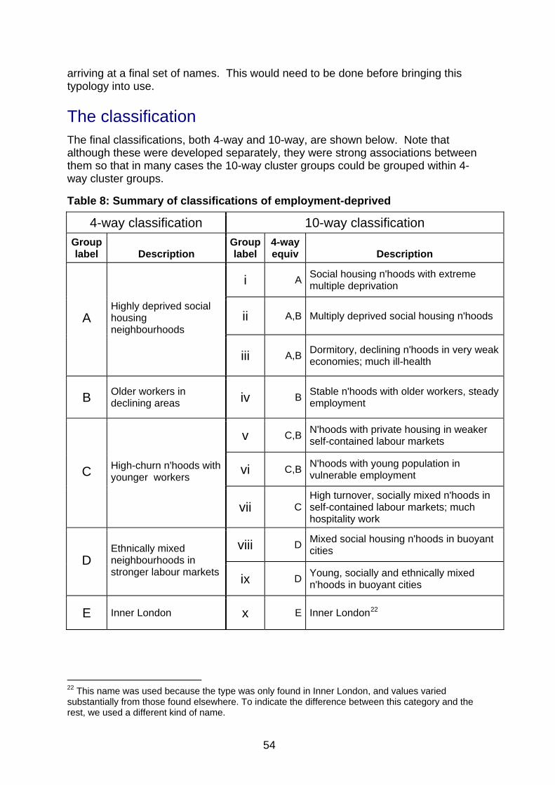
54

arriving at a final set of names. This would need to be done before bringing this typology into use.

The classification The final classifications, both 4-way and 10-way, are shown below. Note that although these were developed separately, they were strong associations between them so that in many cases the 10-way cluster groups could be grouped within 4-way cluster groups.

Table 8: Summary of classifications of employment-deprived

4-way classification 10-way classification Group label Description

Group label

4-way equiv Description

i A Social housing n'hoods with extreme multiple deprivation

ii A,B Multiply deprived social housing n'hoods A Highly deprived social housing neighbourhoods

iii A,B Dormitory, declining n'hoods in very weak economies; much ill-health

B Older workers in declining areas iv B Stable n'hoods with older workers, steady

employment

v C,B N'hoods with private housing in weaker self-contained labour markets

vi C,B N'hoods with young population in vulnerable employment C High-churn n'hoods with

younger workers

vii CHigh turnover, socially mixed n'hoods in self-contained labour markets; much hospitality work

viii D Mixed social housing n'hoods in buoyant cities

D Ethnically mixed neighbourhoods in stronger labour markets ix D Young, socially and ethnically mixed

n'hoods in buoyant cities

E Inner London x E Inner London22

                                                       22 This name was used because the type was only found in Inner London, and values varied substantially from those found elsewhere. To indicate the difference between this category and the rest, we used a different kind of name.

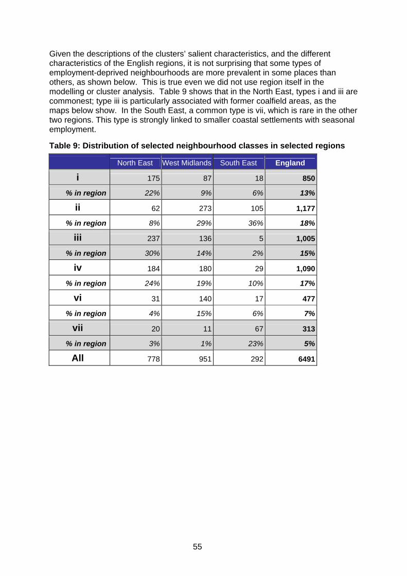
55

Given the descriptions of the clusters’ salient characteristics, and the different characteristics of the English regions, it is not surprising that some types of employment-deprived neighbourhoods are more prevalent in some places than others, as shown below. This is true even we did not use region itself in the modelling or cluster analysis. Table 9 shows that in the North East, types i and iii are commonest; type iii is particularly associated with former coalfield areas, as the maps below show. In the South East, a common type is vii, which is rare in the other two regions. This type is strongly linked to smaller coastal settlements with seasonal employment.

Table 9: Distribution of selected neighbourhood classes in selected regions

North East West Midlands South East England

i 175 87 18 850

% in region 22% 9% 6% 13%

ii 62 273 105 1,177

% in region 8% 29% 36% 18%

iii 237 136 5 1,005

% in region 30% 14% 2% 15%

iv 184 180 29 1,090

% in region 24% 19% 10% 17%

vi 31 140 17 477

% in region 4% 15% 6% 7%

vii 20 11 67 313

% in region 3% 1% 23% 5%

All 778 951 292 6491

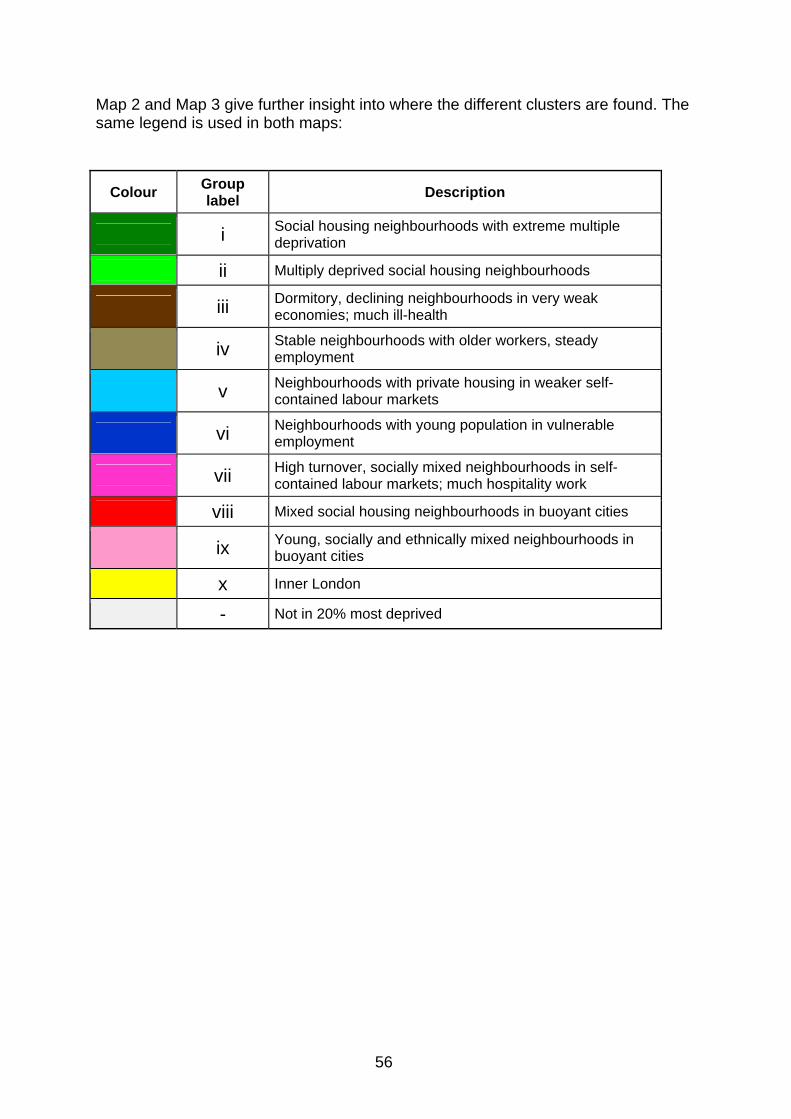
56

Map 2 and Map 3 give further insight into where the different clusters are found. The same legend is used in both maps:

Colour Group label Description

i Social housing neighbourhoods with extreme multiple deprivation

ii Multiply deprived social housing neighbourhoods

iii Dormitory, declining neighbourhoods in very weak economies; much ill-health

iv Stable neighbourhoods with older workers, steady employment

v Neighbourhoods with private housing in weaker self-contained labour markets

vi Neighbourhoods with young population in vulnerable employment

vii High turnover, socially mixed neighbourhoods in self-contained labour markets; much hospitality work

viii Mixed social housing neighbourhoods in buoyant cities

ix Young, socially and ethnically mixed neighbourhoods in buoyant cities

x Inner London

- Not in 20% most deprived

57

Map 2: Distribution of cluster groups in the north

Map 3: Distribution of cluster groups in Tyneside and Teesside

Testing the classification With the classification developed and mapped, we tested its usefulness in several different ways. Some of the tests involve data analysis, to see whether the typology distinguishes groups of areas which share characteristics of policy interest, and whether it is more sensitive to the policy domain than existing neighbourhood

58

classifications such as the Output Area Classification. The typology was also presented to potential policy users and analysts to get their qualitative feedback.

Does the typology identify areas with characteristics of policy interest?

Using cluster analysis means that the groups are distinguished from one another by the variables used to build the clusters. So, as shown above, the groups differ in their typical shares of housing tenures. The classification is much more useful if the groups differ in other characteristics that may be of policy interest but which were not used in generating the classification itself.

A first test of this is in describing the clusters. As an example, we found that one of the groups (vii) was characterised by high levels of employment in the hotels and restaurants sector. This was despite the fact that neither this sector of employment nor characteristics that might be associated with it, such as seasonal unemployment, were part of the cluster analysis.

The health condition by which recipients of Incapacity Benefit are made unable to work is of potential interest in policy planning and targeting. An intervention might offer a therapeutic programme for a particular type of condition, combined with support and incentives to encourage a return to economic activity. We looked at whether the clusters were associated with particular health conditions among Incapacity Benefit claimants (Figure 7, Figure 8).

Figure 7: Average number of Incapacity Benefit claimants with mental conditions in different groups

59

Figure 8: Average number of Incapacity Benefit claimants with musculoskeletal conditions in different groups

These charts show that musculoskeletal conditions are found in greatest number in types iii and iv – particularly associated with coalfield areas and manufacturing towns, whereas mental conditions are prevalent in coastal towns (vii) and inner London (x). Group i (social housing with extreme multiple deprivation) has high numbers of both conditions.

An alternative would be to do univariate analysis and mapping of Incapacity Benefit conditions to identify areas for potential intervention. With the classification, however, the information about the incidence of conditions is linked to a bundle of other information about typical neighbourhood characteristics – housing tenure, demographics, labour market context and so on – which may be important considerations in policy design.

Does it offer anything over existing typologies?

We compared how each Lower Super Output Area was classified by the bespoke worklessness typology to its group in the freely available Output Area Classification for Lower Super Output Areas. We wanted to see whether the bespoke typology drew distinctions that were already picked up by the Census-based Output Area Classification.

All of the 20 Output Area Classification groups for Lower Super Output Areas have some neighbourhoods which are in the 20% most deprived. Some Output Area Classification groups, such as ‘Affluent Urban Commuter’, ‘Farming and Forestry’ and ‘Well-off Mature Households’ have very few. The Output Area Classification group with the most highly deprived neighbourhoods is ‘Struggling Urban Families’, 89% of whose members are included (see Table 10). Apart from that, only two other Output Area Classification groups – ‘Blue Collar Families’ and ‘Multicultural Inner City’ – have more than half their members among the most deprived. This suggests

60

that for targeting policy on the areas with greatest need, the Output Area Classification alone would not be sufficient. The Index of Multiple Deprivation would need to be used instead, or in addition.

Table 10: Cross-classification of the bespoke worklessness typology with selected Output Area Classification groups.

Worklessness group

Output Area Classification group

% of OAC group that is highly

deprived

A high dep soc hsg

B older

workers

C high

churn younger

D eth mix, buoyant

E inner

london

Blue Collar Urban Families 64% 756 733 19 22 0

Educational Centres 11% 4 0 34 11 0

Multicultural Inner City 63% 33 20 45 588 99

Multicultural Suburbia 47% 159 150 107 123 2

Multicultural Urban 34% 25 136 228 31 0

Resorts and Retirement 26% 17 45 240 6 0

Small Town Communities 14% 15 228 13 5 0

Struggling Urban Families 89% 1232 440 58 65 0

Urban Terracing 27% 4 143 273 3 0

Note: Only Output Area Classification groups with at least 10% of Lower Super Output Areas in most employment deprived are shown.

Comparison of the Output Area Classification and bespoke groups for the most deprived neighbourhoods shows some correspondences. Bespoke group D (‘ethnically mixed areas in buoyant cities’) matches well with the Output Area Classification class ‘Multicultural inner city’. However, most of the Output Area Classification groups are spread across several bespoke typology groups, and vice versa. The bespoke typology is more sensitive than the Output Area Classification to place characteristics specifically linked to work and worklessness. The Output Area Classification is based only on neighbourhood characteristics, whereas the bespoke typology also reflects differences in the labour market context of neighbourhoods.

How important is perfecting the model?

A distinctive feature of the example is the use of regression models to select variables for clustering. This does entail greater complexity. Multi-level modelling offers a wide range of ways of representing relationships between variables and

61

spatial levels. In a model with many predictor variables, the potential configurations are near limitless. Similarly, a large number of diagnostic tests and corrections are available. The question arises of how ‘good’ a model ought to be.

Modelling can be extremely time-consuming, and in a complex social domain with sometimes imperfect data, there will not be a single perfect model that can be achieved. In this example, although there is inherent interest in the models’ results, the purpose is ultimately to produce a classification. The models are a means to base the classification on variables that explain employment deprivation, and for the weights given to different characteristics (neighbourhood population composition, housing, labour market features) to roughly approximate their ‘real-world’ importance. Different ways of specifying the model produced different estimates, but the broader balance and mix of variables that guide the eventual classification changed little. In addition, the more complex a model’s structure, the harder its results become to interpret, especially for non-specialists.

Feedback from policy users

The bespoke classification was also evaluated in discussion with potential users, firstly with a small group of DCLG policy users working in the specific field, and then in a larger seminar with users and analysts from several departments.

Policy users felt that the classification ‘made sense’ and fitted with existing understandings and analyses. They felt it identified characteristics of neighbourhoods that are considerations in policy development. The approach was particularly welcomed for drawing together neighbourhood and regional features and making the case that both spatial levels mattered.

Several users commented on the importance of description and naming and felt that the typology would benefit from further characterisation of each cluster.

An important issue identified by potential users was the trade-off between the simplicity of classifications with few groups and the sophistication and sensitivity of those with many. For the bespoke typology, some felt that the 4-way classification was an over-simplification which grouped some heterogeneous neighbourhoods together. Conversely, the 10-way classification was seen by some as overly complex, with the differences between some groups not clear. Some suggested that a classification with six to eight main groups would offer a balance.

Conclusion This example demonstrated the development of a neighbourhood-level classification suited to policy analysis and planning. A classification was able to provide a simplified but nuanced view of a complex and multidimensional policy issue, and the groups made sense to potential users. The bespoke typology distinguished groups of neighbourhoods with characteristics of interest to policy, and sorted neighbourhoods in a novel way compared to an existing generic typology (Output Area Classification). Using multi-level modelling to select the variables for the classification makes the process more complex, but provides an effective way of dealing with the many competing explanations of employment deprivations.

62

SECTION 4

Worked example 2: Identifying local authorities with similar contexts to aid performance comparison

Introduction This section provides a worked example of the development of a classification to aid in the comparison of local authority performance on National Indicators.

We first work through the checklist of issues developed in Section 2 to decide what kind of a classification is needed and whether there are existing products available that might be suitable. We provide references so that readers can refer back to more detail on these issues.

We then set out the steps followed in developing the classification, highlighting methodological considerations.

Third, we demonstrate the resulting classification.

Fourth, we evaluate the robustness of the classification.

Box 10 provides a summary of this section of the toolkit.

Annex D shows the methodological steps in more detail for readers who are interested in applying the classification for policy purposes or who wish to replicate the method.

63

Box 10: Summary of local authority worked example

The Local Analysis and Delivery Unit at DCLG is responsible for monitoring the performance of local authorities on the National Indicators. A key issue is to understand which authorities face similar contexts, in order to know whether performance should be considered in line or out of line with that of other similar authorities.

National Indicators cover many aspects of local authority performance and local outcomes, from the efficiency of planning processes to levels of worklessness. This example explores whether it is appropriate to use existing generic classifications or whether bespoke classifications are necessary to compare performance on different National Indicators. We develop two bespoke classifications for different sets of National Indicators, and compare them with existing classifications, to see whether they predict outcomes more closely. Because the goal is fair performance comparison, we adopt a nearest neighbour approach.

The coverage of the model is England, corresponding with policy jurisdiction in this area. The spatial unit is the local authority. Since some National Indicators are the responsibility of counties and some of districts, we develop one typology at each scale, for illustration purposes. At each of these scales, other classifications exist and are used by other government departments. However, it is unclear whether these are appropriate. The constituent variables might be considered too specific or too generic. There is a reliance on 2001 Census data. Some are data-driven, whilst others are theory-driven but in relation to different outcomes from the ones the Local Analysis and Delivery Unit wants to look at. We therefore decide to develop theory-driven models, including relevant variables for each of the sets of National Indicators we explore.

For each of the two examples, we identify a selection of relevant variables. On each variable we calculate the distance between any given authority and all others, and combine scores for all variables, with no weighting. This identifies the nearest neighbours for each authority. We test the model by working out how well it predicts differences in actual performance on the specific National Indicators, compared with other existing tools and with just comparing each authority to the national average. We find that the bespoke model has similar performance to that of existing tools which were not specifically designed in relation to these indicators.

The conclusion from this exercise is that bespoke nearest neighbour models for local authority comparison can be developed within about a month’s work for one analyst with expertise in the statistical methods involved and knowledge of the data sources. This is not a light undertaking for a government department, although it is modest by comparison with some eternally commissioned analyses. The main value of such models is that they have value in being seen to be fine-tuned and therefore fairer than more generic classifications or one developed for other purposes. However, in statistical terms, relatively little additional accuracy is gained from the investment in bespoke classifications. Existing tools are likely to do the job just as well.

64

Stage 1: Assessment of requirements

Box 11: Checklist of questions before developing a classification

1. For what policy purpose is the classification needed?

2. What kind of classification is best suited to this purpose?

3. What coverage and spatial scale is appropriate?

4. What existing tools and products exist at this coverage and spatial scale?

5. Is it necessary to develop a bespoke classification?

6. To what extent should the classification be theory-led or data led?

7. What kinds of variables should be included?

For what policy purpose is the classification needed?

The way in which public bodies, including local authorities, perform their statutory duties is subject to external scrutiny and audit. One element of the performance management regime for local authorities is the collation of quantitative indicators of outcomes in fields in which local authorities work. In 2007, a unified set of 198 indicators for English local authorities were announced, covering domains such as ‘Stronger and Safer Communities’ and ‘Children and Young People’. The indicators were largely drawn from existing sample survey and administrative data sources. They are known as the National Indicator set (NI set or NIs). The Local Analysis and Delivery Unit in DCLG is responsible for monitoring local authority performance on these indicators.

One way in which an indicator may be used is to see whether, in any given local authority, it is changing in the desired direction over time – are crime rates falling in X? Are examination results improving in Y? Both local practitioners and external auditors may also find it useful to compare the same indicator across several authorities – perhaps to identify authorities whose policies and administration are especially effective, or that are not reaching expected standards.

Comparing indicator scores between authorities is made more complex by the fact that almost all indicators are determined not only by an authority’s effectiveness, but in large part by the characteristics of the area it administers. For example, children with parents in managerial and professional occupations consistently attain higher scores in school examinations. Therefore, local authorities where many residents work in such occupations would be expected to perform better than others on an examinations indicator. This better performance would not necessarily reflect more effective administration of educational services in the area – an authority with a different occupational structure might be more effective, but still have lower pass rates. What is needed, therefore, is some way to identify ‘fair’ comparisons between authorities.

65

This is illustrated by Figure 9 below, which allocates a score on a scale of 0-100 to five fictional authorities on a fictional indicator. The panel on the left shows raw performance scores. On this basis, we would say that ‘C’ shire County Council is by far the best performer, and Metropolitan Borough ‘E’ the least. However, accounting for context provides a very different picture. In the right hand panel, we see that ‘C’ shire County Council actually has a very much more favourable context than the other authorities and that this accounts for most of the raw performance variation, although not all. ‘E’ Metropolitan Borough turns out to have a much less favourable context that all the others. Once this is taken into account, it emerges as a relatively strong performer.

Figure 9: The Importance of context in local authority performance

0 50 100

London Borough  of "A"

West "B" District

"C"'shire County 

City of "D" UA

"E" Met Borough NI Score

0 50 100

London Borough  of "A"

West "B" District

"C"'shire County 

City of "D" UA

"E" Met Borough

ContextPerformance

Having a fair peer group is useful both for local authorities themselves, who wish to track their own progress, and for those, like the Local Analysis and Delivery Unit, who are involved in the external evaluation of delivery. This means finding authorities which are as like each other as possible on relevant factors. However, the breadth of the National Indicator set makes this complicated. Can we assume that a local authority’s closest comparator for a particular National Indicator or domain (say Children and Young People) is also its closest comparator when it comes to comparing performance on housing, transport or community cohesion? This would depend on whether certain major underlying factors, such as levels of deprivation, underpin performance on all indicators or whether more specific factors are influential. There is a pragmatic issue in that some of the National Indicators relate to the functions of district councils and unitaries, while others relate to the functions of county councils and unitaries.

In this example, we develop a model to identify relevant comparators on two sets of indicators, from the Stronger Communities and Local Economy domains of the National Indicator set. Stronger Communities was selected in order to illustrate a classification at the county/unitary level, while Local Economy illustrates comparison at the district/unitary level.

66

These domains are considered as sets, and local authorities select indicators from within them. What is needed is therefore a way of comparing authorities on the domains, rather than on individual indicators. It would clearly be impractical to develop 198 bespoke classifications for comparison purposes.

In consultation with the Local Analysis and Delivery Unit, we selected a small number of indicators from within each domain which are widely used by local authorities and which together reflect the scope of the domain. Similar selections could be made from the other domains.

Table 11: Selected indicators from selected domains of the National Indicator set

Stronger Communities Local Economy

NI 001 % of people who believe people from different backgrounds get on well together in their local area

NI 151 Overall Employment rate (working-age)

NI 002 % of people who feel that they belong to their neighbourhood

NI 152 Working age people on out of work benefits

NI 004 % of people who feel they can influence decisions in their locality

NI 171 New business registration rate

NI 005 Overall/general satisfaction with local area

NI 173 Flows on to incapacity benefits from employment

NI 007 Environment for a thriving third sector

NI 009 Use of public libraries

What kind of classification is best suited to this purpose?

A nearest neighbour model is most appropriate for this purpose because:

• It is fairest. Local authorities will always be compared with the other authorities that are most similar to them.

• It is consistent with the kind of use to which the classification will mostly likely be put. Typically, scrutiny of performance and benchmarking exercises start with one authority and look outwards to find comparators, rather than starting with an overall national pattern.

• It is easily used and manipulated to identify more or fewer comparators e.g. the five nearest neighbours, the ten nearest neighbours

What coverage and spatial scale is appropriate?

Liaison with and monitoring of local government is a devolved function in the UK, with each country having responsibility for its own authorities. The classification must therefore cover England only.

‘Stronger Communities’ are compared for district and unitary authorities, ‘Local Economy’ for counties and unitaries.

67

What existing tools and products exist at this coverage and spatial scale?

There already exist several schemes for identifying comparator groups for local authorities including:

• The Chartered Institute of Public Finance and Accountancy’s nearest neighbour model

• The Department for Children, Schools and Families’ nearest neighbour model

• Home Office research to identify peers for Crime and Disorder Reduction Partnerships

• The Office for National Statistics Census-based classification of local authority districts.

(See Annex A for details of these.)

Is it necessary to develop a bespoke classification? As we are interested in using a nearest neighbour model, the Office for National Statistics classification is not appropriate for this purpose. However, the nearest neighbour models developed by the Chartered Institute of Public Finance and Accountancy and other government departments are potential tools. Discussion with policy colleagues revealed uncertainty on whether such tools would be suitable. The broadest classification (that of the Chartered Institute of Public Finance and Accountancy) was regarded as potentially too broad for assessing the context for performance on specific domains. It includes indicators of local authority resources as well as socio-economic context. The bespoke classifications designed for specific purposes were seen as potentially too specific to be applicable to other domains. For example, the Department for Children, Schools and Families’ one is strongly loaded towards family circumstances and the resources available to families with children (Table 12).

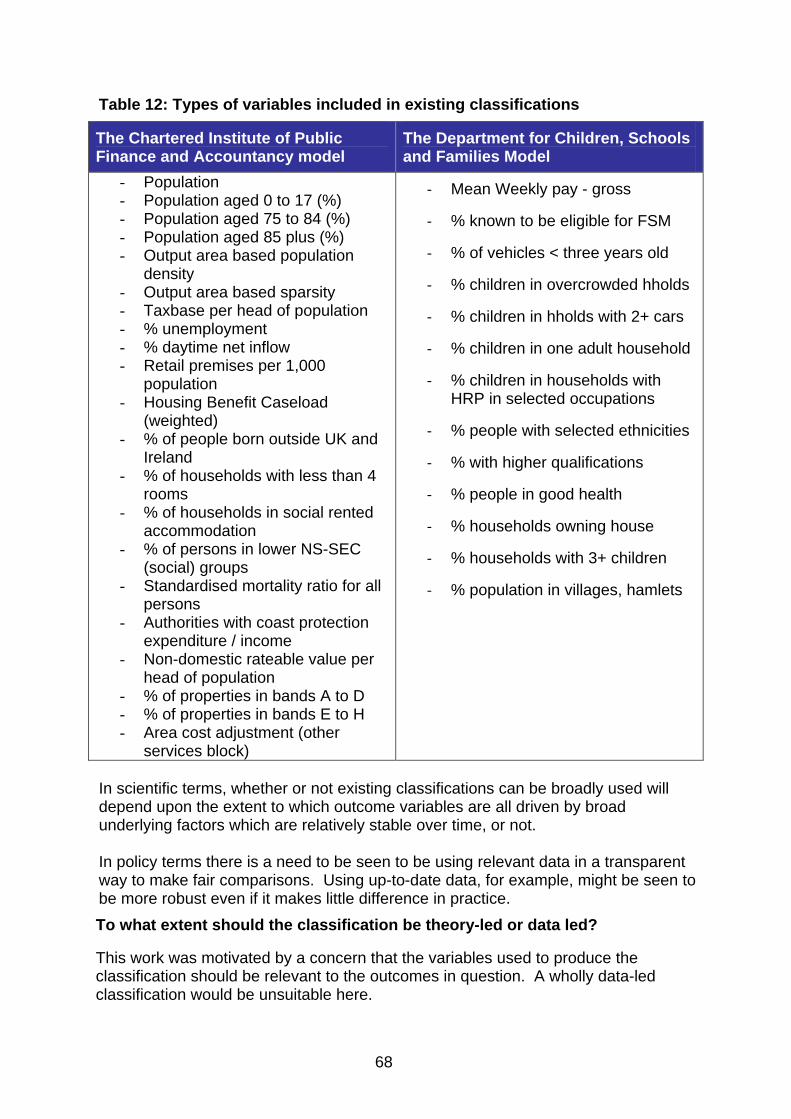
68

Table 12: Types of variables included in existing classifications

The Chartered Institute of Public Finance and Accountancy model

The Department for Children, Schools and Families Model

- Population - Population aged 0 to 17 (%) - Population aged 75 to 84 (%) - Population aged 85 plus (%) - Output area based population

density - Output area based sparsity - Taxbase per head of population - % unemployment - % daytime net inflow - Retail premises per 1,000

population - Housing Benefit Caseload

(weighted) - % of people born outside UK and

Ireland - % of households with less than 4

rooms - % of households in social rented

accommodation - % of persons in lower NS-SEC

(social) groups - Standardised mortality ratio for all

persons - Authorities with coast protection

expenditure / income - Non-domestic rateable value per

head of population - % of properties in bands A to D - % of properties in bands E to H - Area cost adjustment (other

services block)

‐ Mean Weekly pay - gross

‐ % known to be eligible for FSM

‐ % of vehicles < three years old

‐ % children in overcrowded hholds

‐ % children in hholds with 2+ cars

‐ % children in one adult household

‐ % children in households with HRP in selected occupations

‐ % people with selected ethnicities

‐ % with higher qualifications

‐ % people in good health

‐ % households owning house

‐ % households with 3+ children

‐ % population in villages, hamlets

In scientific terms, whether or not existing classifications can be broadly used will depend upon the extent to which outcome variables are all driven by broad underlying factors which are relatively stable over time, or not. In policy terms there is a need to be seen to be using relevant data in a transparent way to make fair comparisons. Using up-to-date data, for example, might be seen to be more robust even if it makes little difference in practice. To what extent should the classification be theory-led or data led?

This work was motivated by a concern that the variables used to produce the classification should be relevant to the outcomes in question. A wholly data-led classification would be unsuitable here.

69

On the other hand, there is no one clear body of theory that indicates definitively which kinds of context lead to particular challenges for local authorities on these indicators. It is not simply a matter of defining ‘types’ on the basis of prior knowledge (a purely theory driven approach).

In this example, we demonstrate an approach that is mainly theoretically driven, but tested empirically in a straightforward, replicable and transparent way. We make principled decisions to include context variables specifically relevant to each domain, based on our own knowledge of the literature in this field and discussions with policy colleagues. We then experiment with entering different numbers and combinations of variables into the models in order to understand which variables have most impact on the classification and produce the best fit with actual performance.

What kinds of variables should be included?

This example was designed to demonstrate the application of a relatively straightforward approach to designing a classification. Clearly, provided that variables are carefully selected and validated, and that they are all measuring distinctly different things, one would expect a model with more variables to have more power than one with fewer, but there is a trade-off between improved accuracy and simplicity and transparency. We decided in each case to limit the number of variables to fewer than ten. As part of the testing process, we examined the effect of using fewer variables than this.

Stronger communities

In this example, the classification is designed to help us understand which local authorities have contexts which would lead to different kinds of attitudes and behaviours.

In considering which variables to include, we need to theorise which other kinds of contextual variables might be related to these characteristics.

Analysis of the Citizenship Survey23indicates that attitudes towards community vary substantially by age, ethnicity and social class. We would therefore expect that the demographic and socio-economic composition of an area would be highly influential on these outcomes. Environmental and geographical characteristics may also influence attitudes and opportunities for interaction.

Table 13 shows the selection of variables, and the most appropriate and up-to-date data source. This is a much simpler approach than the one adopted in Section 3 and does not involve consideration of different spatial scales. All the variables are at the local authority level. Note that:

• A variety of sources has been used.

• The most recent data possible has been used, although for some variables, this is the 2001 Census. The most up-to-date sources date from 2008 and 2009. The inevitable lag in the production of statistics means that no classification can actually be truly current.

                                                       23 Laurence, J. and Heath, A. (2008) Predictors of community cohesion: multi-level modelling of the 2005 Citizenship Survey. London: DCLG.

70

• Although institutional variables (such as the numbers of libraries) are clearly relevant to the outcomes, we exclude them here because they are elements of local authority performance, whereas we are interested here in identifying aspects of context that impact on performance, not performance itself.

Table 13: Variables included in the stronger communities model

Context Variables Rationale Source/date

Compositional Variables

% adults aged under 30

Younger adults may be less likely to be involved in local area

MYE population estimates 2008

% households which have dependent children

Children possible stimulus for adult engagement and relationships in local area

Census 2001

% Managerial & Professional

Higher social classes may be likelier to use libraries and cultural facilities

Census 2001

Ethnic diversity index (Simpson’s)

High ethnic homogeneity, and some kinds of diversity, correlated with some cohesion measures in survey data

Derived from Census 2001

Unemployment rate Literature suggests poverty damages cohesion LFS 2009

Geographical and Environmental Variables

% flatted housing Built form may influence opportunities for informal interaction

Census 2001

Local economy

Theory suggests that local economic indicators are influenced both by supply-side and demand-side factors.

Supply-side factors relate to the skills and attributes of the work force. Thus we include compositional variables relating to people of working age. Demand-side measures capture the nature of the local economy. It is widely argued that the relevant scale at which to consider labour demand is not the local authority (because people are not constrained by administrative boundaries) but the wider labour market, incorporating possibilities for travelling to jobs and the nature of supply-chain relationships. Strong sub-regional economies generate labour demand even if there are few jobs in the immediate vicinity. Geographical variables indicating the degree of connectivity to these opportunities can then be incorporated

71

Table 14: Variables in the local economy model

Context Variables Rationale Source/date

Supply side variables

% adults no qualifications 2001

Job opportunities for resident labour depend on skills and qualifications

Census 2001

Long-term sickness related economic inactivity

High sick rates indicator of economically inactive adults distant from labour market

Proportion of working-age population claiming IB/ESA for 1+ years

Demand-side variables

Working-age population

Scale of local authority area labour force MYE estimates 2008

% employed in manufacturing

Resident workforce exposure to a potentially vulnerable / high unemployment sector

Census 2001

% employed in public sector services

Resident workforce exposure to a counter-cyclical sector Census 2001

% employed in private sector services

Resident workforce exposure to a growing sector Census 2001

Gross Value Added per capita in NUTS3 area24

Relative value of economic output in wider economic area Regional Accounts, 2008

Self-employed High rates of self-employment may indicate more opportunity for entrepreneurialism (Although this may also indicate insecure employment in some areas)

Census 2001 or LFS

Jobs density in NUTS3 area

Measure of wider area demand for labour – use pre-recession figure

NOMIS 2007

Geographical Variables

% working residents working outside

Identify dormitory areas Census 2001

% local workforce not resident

Identify central employment areas Census 2001

                                                       24 Note this is used as an approximate indicator only; figures at this spatial level are somewhat unreliable.

72

Methodological steps Testing and selection of variables

This example is designed to demonstrate a relatively straightforward approach to typology construction. Having chosen the variables, we included them all without applying further tests to determine the extent of colinearity or relationship to outcomes. We applied tests of the relative importance of the variables at a later stage.

Calculating similarity and distance

The variables are used to calculate how near (similar) each authority is to every other.

Figure 3 illustrates how nearness is calculated for two variables. Each variable is an axis along which distance is measured, and a total distance between two points can thus be calculated. The same approach can be applied to any number of variables; Annex D provides more information.

Once the distance between every pair of neighbours is known, each authority’s nearest neighbours are simply those with the smallest distance. These are the most similar authorities.

The classification The output from the classification is a list of the nearest neighbours for each local authority. This list is available separately for the two bespoke nearest neighbour models discussed here. Examples of the nearest neighbours for two authorities are shown below, with comparisons to their nearest neighbours as identified by the Chartered Institute of Public Finance and Accountancy’s (CIPFA) tool. Bradford has many of the same neighbours under both models, although their positions differ. Only a few of North Somerset’s neighbours are common to CIPFA and the bespoke model.

 

73

Table 15: Nearest neighbours for Bradford and North Somerset, from bespoke and CIPFA nearest neighbour models

Bradford MD North Somerset UA Bespoke model CIPFA Bespoke model CIPFA

1 Coventry Kirklees North Yorkshire Poole 2 Blackburn with

Darwen Coventry Gloucestershire Isle of Wight

3 Luton Bolton Poole Bath & NE Somerset

4 Rochdale Oldham West Sussex East Riding of Yorkshire

(mos

t sim

ilar)

5 Barking and Dagenham

Rochdale East Riding of Yorkshire

South Gloucestershire

6 Middlesbrough Luton Herefordshire Solihull 7 Peterborough Derby Somerset Stockport 8 Hillingdon Walsall Suffolk Southend-on-Sea 9 Derby Blackburn with

Darwen Cheshire Torbay

(less

sim

ilar)

10 Walsall

Calderdale East Rutland York

The classification can be used to select comparison groups. For example, the performance of any given local authority can be compared with its ten nearest neighbours. Alternatively, local authorities could be compared only with others where the combined score is lower than a certain value. Some local authorities would have fewer comparators than others, but each would be being compared only with ones that are truly comparable.

Testing the classification Testing overall predictive power, compared with other classifications

The key question we sought to explore in undertaking this work is whether developing a bespoke classification with carefully selected relevant variables provides a closer comparison than using existing nearest neighbour models.

To test this we applied a method used by the National Foundation for Educational Research in testing the nearest neighbour model they developed for the Department for Children, Schools and Families. The method is based on the premise that the model should have some predictive power in relation to the outcomes that are being measured. We would expect that authorities with similar contexts would have similar outcomes on the National Indicators. Nearest neighbour models can therefore be compared by calculating the mean difference between an authority and any given number of its neighbours, on the outcomes in which the client is interested. A smaller score would indicate a closer comparison.

We compare our Stronger Communities model (with either 5 or 15 neighbours) against those developed by CIPFA (5 or 15) and the Department for Children, Schools and Families (5 or 10),25 in relation to their predictive power on the Stronger                                                        25 The Department for Children, Schools and Families classification identifies 10, not 15 nearest neighbours.

74

Communities National Indicators. We also compare it to what would happen if each authority were compared just with the national average, or with all the other authorities in its region. We standardise these results so that comparing with the national average has a value of 1 and all others a percentage of 1.

The results are shown in

Table 16. They indicate that all of the models perform much better than just comparing with the national average. However, there is little to choose between them. Comparing with the five closest neighbours on the Chartered Institute of Public Finance and Accountancy model or the five closest on the Department for Children, Schools and Families model would be, on average, as good a comparison as the one provided by our bespoke model, even though these other models are not specific to Stronger Communities outcomes.

Table 16: Relative performance of different nearest neighbour models

Standardised value Raw value

National Average 1.00 0.997

CIPFA-15 0.71 0.711

CIPFA-5 0.58 0.581

DCSF-10 0.54 0.541

DCSF-5 0.56 0.555

Our Model-15 0.55 0.547

Our Model-5 0.57 0.570

Changing the component variables

We can also use this method to revisit and fine tune our own model. Which combination of variables produces a model with the best predictive power? How much can be achieved by a classification just based on one or two variables?

For the Stronger Communities model, testing each variable in our model separately, we find that the ethnic diversity score produces the best single variable performance. However, this is little better than just comparing with the national average (Table 17). Adding one more variable (the proportion in managerial or professional occupations) improves the power of the model considerably. Using just two variables produces a nearest neighbour model which is not a great deal worse than using six and is still substantially better than just comparing to the national average, especially when wider comparisons are wanted (to compare with the nearest fifteen authorities not just the nearest five).

75

Table 17: Testing the model with just one or two variables

Model Score Variables (our models only)

National Average 1.00

CIPFA-5 0.58

DCSF-5 0.56

Our Full Model- 5 0.57 age < 30, flats, ethnic div, unemp, dep children, mgr/prof

Our Single Variable Model-5 0.94 ethnic diversity

Our Single Variable Model-15 0.79 ethnic diversity

Our dual variable model - 5 0.67 ethnic div, mgr/ prof

Our dual variable model -15 0.61 ethnic div, mgr/ prof

These results tend to suggest that investment in bespoke models of great complexity is probably not wise, as they do not provide substantially better comparisons than existing tools or more simple models capturing key characteristics.

‘Road testing’

Finally, we ‘road-tested’ the classification on staff of the Local Analysis and Delivery Unit and with a wider range of policy colleagues and analysts at a workshop hosted by DCLG. The finding that domain-specific bespoke neighbour models did not perform better than generic or wrong-domain models was of particular interest. Analysts suggested a number of further metrics that might be useful in evaluating techniques for comparator groups, such as indicators of the range within comparator groups, as well as the relative means. Another suggestion was to see how stable the implied ‘performance’ of each authority was as the neighbour model, and thus its comparators, changed.

Conclusion This worked example was designed to address concerns that existing classifications designed to compare local authority performance might not be fit for the purpose of examining performance on specific National Indicators. We demonstrate that a bespoke classification can be developed in a relatively modest amount of time. We produced models for two sets of indicators within approximately 20 days. However, the gains from doing this are slight, in statistical terms. This suggests that there are broad contextual factors that influence outcomes across the spectrum, rather than very specific contextual factors affecting very specific outcomes. The implication of this is also that there may be considerable stability in neighbours over time. Although absolute values may change, necessitating up-to-date data, relative positions may change a lot less. Bespoke nearest neighbour models clearly have political value in being transparent, specific and up-to-date. The value of this needs to be traded off against the cost of their development.

76

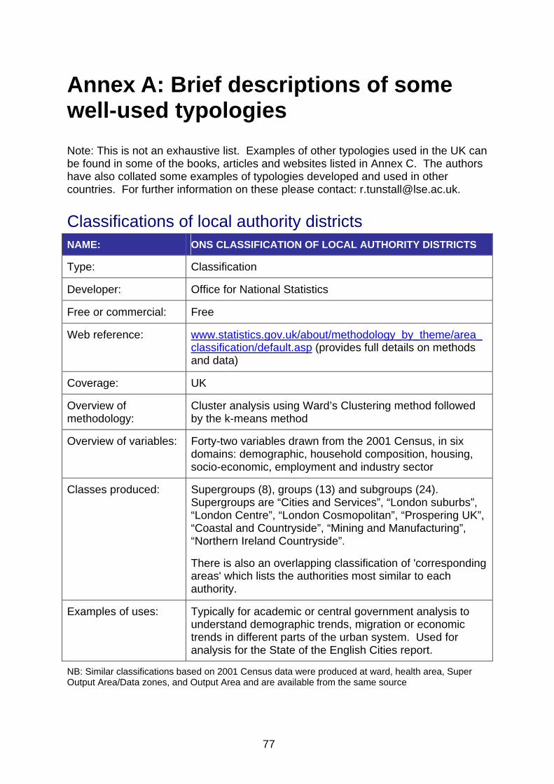
77

Annex A: Brief descriptions of some well-used typologies Note: This is not an exhaustive list. Examples of other typologies used in the UK can be found in some of the books, articles and websites listed in Annex C. The authors have also collated some examples of typologies developed and used in other countries. For further information on these please contact: r.tunstall@lse.ac.uk.

Classifications of local authority districts NAME: ONS CLASSIFICATION OF LOCAL AUTHORITY DISTRICTS

Type: Classification

Developer: Office for National Statistics

Free or commercial: Free

Web reference: www.statistics.gov.uk/about/methodology_by_theme/area_classification/default.asp (provides full details on methods and data)

Coverage: UK

Overview of methodology:

Cluster analysis using Ward’s Clustering method followed by the k-means method

Overview of variables: Forty-two variables drawn from the 2001 Census, in six domains: demographic, household composition, housing, socio-economic, employment and industry sector

Classes produced: Supergroups (8), groups (13) and subgroups (24). Supergroups are “Cities and Services”, “London suburbs”, “London Centre”, “London Cosmopolitan”, “Prospering UK”, “Coastal and Countryside”, “Mining and Manufacturing”, “Northern Ireland Countryside”.

There is also an overlapping classification of 'corresponding areas' which lists the authorities most similar to each authority.

Examples of uses: Typically for academic or central government analysis to understand demographic trends, migration or economic trends in different parts of the urban system. Used for analysis for the State of the English Cities report.

NB: Similar classifications based on 2001 Census data were produced at ward, health area, Super Output Area/Data zones, and Output Area and are available from the same source

78

NAME: CIPFA NEAREST NEIGHBOURS

Type: Nearest Neighbour Model

Developer: Chartered Institute for Public Finance and Accountancy

Free or commercial: Free

Web reference: www.cipfastats.net/ (provides full info on methodology and variables)

Coverage: England

Overview of methodology:

All variables standardised. Euclidean distances calculated between each authority and each other on each variable. Distances summed across variables and rebased so that 1 represents the farthest neighbour

Overview of variables: Demographic variables, sparsity, but also indicators of density of commercial activity, commuting, visitor populations and whether on coast or prone to flooding. Designed to identify challenges to local authority performance.

Classes produced: NA

Examples of uses: Used by local authorities for benchmarking purposes. Used by Audit Commission for Value for Money Profiles

NAME: HOME OFFICE FAMILY GROUPS

Type: Classification

Developer: Home Office

Free or commercial: Free

Web reference: http://rds.homeoffice.gov.uk/rds/prgpdfs/brf300.pdf

Coverage: England

Spatial Scale: Crime and Disorder Reduction Partnerships (CDRPs)

Overview of methodology:

Cluster analysis using k-means and the more recent ‘self organising map’ (SOM) which works more on identifying the main patterns occurring in the data. Methods were combined to produce optimum fit

Overview of variables: Demographic and economic variables and also indicators of size of daytime populations and length/type of roads. Designed to reflect challenges for policing and community

79

safety.

Classes produced: Thirteen ‘families’ (numbered 1 to 13)

Examples of uses: Used by Home Office to benchmark performance of CDRPs. More recently the Home Office has moved to a nearest neighbour model

NAME: CHILDRENS’ SERVICES STATISTICAL NEIGHBOURS BENCHMARKING TOOL

Type: Nearest Neighbour Model

Developer: Department for Children, Schools and Families

Free or commercial: Free

Web reference: www.data4nr.net/outbound/692/1264/

Coverage: England

Spatial Scale: County/Unitary Authority

Overview of methodology:

All variables standardised. Euclidean distances calculated between each authority and each other on each variable. Distances summed across variables

Overview of variables: Selected on basis of correlation with children’s services outcomes. Includes demographic and economic variables mainly relating to circumstances affecting children (eg household structure, car ownership among families with children)

Classes produced: N/A. Each local authoritycan identify nearest neighbours and also identify those which are ‘close’ ‘somewhat close’ or ‘not close’

Examples of uses: Used to support performance monitoring and inspection on children’s services indicators

NAME: RURAL/URBAN CLASSIFICATION

Type: Classification

Developer: Department for Environment, Food and Rural Affairs

Free or commercial: Free

Web reference: www.defra.gov.uk/evidence/statistics/rural/documents/rural-defn/LAClassifications_technicalguide.pdf

80

Coverage: England

Spatial Scale: Local Authority District

Overview of methodology:

Draws on rural/urban definition of Census Output areas (www.ons.gov.uk/about-statistics/geography/products/area-classifications/rural-urban-definition-and-la-classification/index.html This is used to define classes on the basis of proportion of district population living in Output Areas of these different points. Cut-off points to define classes were in most cases chosen on the basis of evidence (statistical and visual) of a ‘natural break’ in the rank ordered histogram of the relevant distribution.

Overview of variables: NA

Classes produced: “major urban”, large urban”, “other urban”, “significant rural” (between 26 and 50 percent of its population in rural settlements and large market towns), rural-50 (50-to-80% of population living in rural settlements or large market towns), Rural-80 (80% of their population in rural settlements and large market towns)

Examples of uses: Relatively recently developed. Widely used by the Department for Environment, Food and Rural Affairs. Beginning to be matched to major surveys and data sets (e.g. Edubase, Millennium Cohort Study) to provide broad contextual indicators e.g. on school location or location of social housing.

81

Classifications of neighbourhoods NAME: MOSAIC

Type: Classification

Developer: Experian

Free or commercial: Commercial

Web reference: www.business-strategies.co.uk/

Spatial Scale Postcode unit

Coverage UK

Overview of methodology:

Not published

Overview of variables: C400, just over half from census; others include shareholder register, consumer credit data, postal address files, council tax data, edited electoral rolls and lifestyle surveys

Classes produced: 61 types, aggregated into 11 groups: “symbols of success” “happy families”, “suburban comfort” “ties of community” “urban intelligence” “welfare borderline” “ municipal dependency” “blue collar enterprise” “twilight subsistence” “grey perspectives” and “rural isolation”

The classes are classes of people based on the typical characteristics of where they live. Experian has also developed a public sector MOSAIC geared more towards identifying needs for public sector services

Examples of uses Widely used eg to project needs for health services, to assess likely policing demands or fire risk. See case studies at: www.experian.co.uk/www/pages/why_experian/client_case_studies/improve_data_and_data_management.html

NAME: ACORN

Type: Classification

Developer: CACI

Free or commercial: Commercial

Web reference: www.caci.co.uk/acorn

82

Spatial Scale Postcode unit

Coverage UK (although there are specialist ACORNs for Scotland, Ireland and Metropolitan areas

Overview of methodology:

Detail not published

Overview of variables: Over 400. Starts with 35 Census variables but reclassifies according to lifestyle surveys and other government sources.

Classes produced: 5 categories, 17 groups and 56 types. Categories are “wealthy achievers”, “urban prosperity”, “comfortably off”, “moderate means”, “hard pressed”

Examples of uses: Similar uses to those of MOSAIC and OAC

NAME: OUTPUT AREA CLASSIFICATION

Type: Classification

Developer: Dan Vickers (University of Sheffield). Now an Office for National Statistics product

Free or commercial: Free

Web reference: www.statistics.gov.uk/about/methodology_by_theme/area_classification/oa/default.asp

www.sasi.group.shef.ac.uk/area_classification/

Spatial Scale Census Output Areas

Coverage UK

Overview of methodology: Cluster analysis

Overview of variables: 42 Census variables

Classes produced: 7 super groups, 21 groups and 52 sub-groups. Super groups include “multicultural”, “typical traits” “constrained by circumstances”, “prospering suburbs”, “countryside”, “city living”, “blue collar communities”

Examples of uses See http://areaclassification.org.uk/case-studies/

83

NAME: INDICES OF MULTIPLE DEPRIVATION

Type: Multivariate indices

Developer: DCLG

Free or commercial: Free

Web reference: www.communities.gov.uk/communities/neighbourhoodrenewal/deprivation/deprivation07/

Spatial Scale Lower Super Output Areas (LSOAs)

Coverage England (separate indices are available for the other UK countries

Overview of methodology: Indices are combined within domains to produce single summary measures. Where the underlying metric is the same, this can be done simply by summing indicators and dividing by the underlying population at risk. Otherwise factor analysis was used to derive weights for combining indicators. Domain scores are then standardised and transformed and combined into a single index based on theoretical considerations.

Overview of variables: 37 different indicators which cover specific aspects or dimensions of deprivation: Income, Employment, Health and Disability, Education, Skills and Training, Barriers to Housing and Services, Living Environment and Crime

Classes produced: N/A but note that there are separate domains that make up the indices, so rankings can be produced on combinations of different measures

Examples of uses: Very widely used as basis for analysis of trends and distribution (see for example recent report of National Equality Panel). Used for funding purposes by DCLG

84

Annex B: Useful links  

(See also the links to individual classifications in Annex A.)

Articles, books and reports The Association of Public Health Observatories Technical Report on Geodemographic Segmentation www.apho.org.uk/resource/item.aspx?RID=67914

Ashby, D.A. (2005) Policing neighbourhoods: Exploring the geographies of crime, policing and performance assessment. Policing and Society, 15(4), pp.413-447.

Batey, P. and Brown, P. (2007) The spatial targeting of urban policy initiatives: a geodemographic assessment tool. Environment and Planning A, 39, pp.2774-2793. Benton, T., Chamberlain, T., Wilson, R. and Teeman, D. (2007) The Development of the Children’s Services Statistical Neighbour Benchmarking Model: final report. Slough: NFER. Birkin, M. Geodemographics (a presentation which provides a useful introduction to the subject for beginners) www.reallifemethods.ac.uk/training/workshops/geodemographics/documents/birkin-history-geodemographics.pdf Brown, P., Hirschfield, A. and Batey, P. (2000) Adding value to census data: Public sector applications of super profiles geodemographic typology. Journal of Cities and Regions,10, pp.19-32.

Champion, A. Green.A., Owen, D., Ellin, D. and Coombes, M. (1987) Changing Places: Britain’s Demographic, Economic and Social Complexion. London: Edward Arnold.

Defra (2004) Social and Economic Change and Diversity in Rural England: A report by the Rural Evidence Research Centre Birkbeck College, London. London: Department for Environment, Food and Rural Affairs.

Dr Foster Research Ltd and Tetlow Associates Ltd (2007) Guide to Segmentation: Customer Satisfaction Measures for Local Government Services. Prepared for the Local Government Association, Improvement and Development Agency and National Consumer Council. (Shows how classifications can be used to target local authority services or understand the needs of different groups of citizens.) www.lga.gov.uk/lga/aio/37774

Harris, R.J., Sleight, P. and Webber, R. (2005) Geodemographics, GIS and Neighbourhood Targeting: Wiley.

Harris, R., Johnston, R. and Burgess, S. (2007) Neighborhoods, Ethnicity and School Choice: Developing a Statistical Framework for Geodemographic Analysis. Population Research and Policy Review, 26, pp.553-579.

85

Leventhal, B. (1995) Evaluation of geodemographic classifications. Journal of Targeting, Measurement and Analysis for Marketing, 4, pp.173-183. Ojo, A. (2009) A Proposed Quantitative Comparative Analysis for Geodemographic Classifications. Published online by the Yorkshire and Humber Public Health Observatory. www.yhpho.org.uk/resource/item.aspx?RID=10170

Vickers, D.W. and Rees, P.H. (2007) Creating the National Statistics 2001 Output Area Classification. Journal of the Royal Statistical Society Series A, 170(2), pp.379-403.

Vickers, D.W., Rees, P.H. and Birkin, M. (2003) A New Classification of UK Local Authorities Using 2001 Census Key Statistics. Working Paper 03/3. Leeds: School of Geography, University of Leeds.

Vickers, D. (2006) Multi-level Integrated Classifications Based on the 2001 Census. PhD Thesis. Leeds: University of Leeds. www.geog.leeds.ac.uk/people/old/d.vickers/thesis.html

Voas, D. and Williamson, P. (2001) The diversity of diversity: a critique of geodemographic classification. Area, 33, pp.63-76.

Williams, S. and Botterill, A. (2006) Profiling Areas Using the Output Area Classification, Regional Trends, 39, pp.11-18.

Websites Spatial_Literacy.org (A joint initiative of the University of Leicester, University College London and the University of Nottingham) www.spatial-literacy.org

Market Research Society Geodemographics Knowledge Base www.geodemographics.org.uk/index.html

Presentations from a Market Research Society introductory seminar on the techniques of geodemographics www.mrs.org.uk/networking/cgg/cggnov08.htm

The Output Area Classification User Group www.areaclassification.org.uk

Oneplace (website on how local public services and how they are performing: provides information on comparison groups) http://oneplace.direct.gov.uk/aboutthissite/contents/pages/aboutcomparisongroups.aspx

Data4Neighbourhood Renewal (Provides information and links to datasets and tools that can be used for comparison purposes) www.data4nr.net/resources/geographies--benchmarking

86

Annex C: Technical details of development of the typology of workless neighbourhoods  

Overview This appendix provides additional information on the development of the typology of neighbourhood worklessness presented in Section 3 of the toolkit. The final typology was created by using standard cluster analysis techniques. As an interim stage to the classification, a series of regression models were estimated in order to identify neighbourhood and labour market characteristics which are significantly associated with different dimensions of employment deprivation.

This appendix is intended to provide more information on the regression models and cluster analysis, and to permit the findings to be reproduced. It therefore assumes familiarity with the datasets and statistical techniques used. The aim of the project was to demonstrate applications of spatial typologies and describe different methods. The annex therefore notes places where particular decisions were made, and alternative approaches that might be relevant in similar work.

Tools

The estimation of the multi-level models and the cluster analysis was done using R, an open-source statistics package.26 The nlme package was used for the multi-level modelling.27 The code specifying the models, cluster analysis and derived variables is available.

Microsoft Excel was used for some data preparation and formatting of tables of results. The maps were drawn using ArcGIS.

Source data All the base variables and their sources are listed in the table below. The source data for the modelling and clustering exercise were all drawn from publicly-available datasets. They are measured at three spatial levels: Lower Super Output Area, Local Authority District and NUTS3. Local authority boundaries are those that applied before the 2009 reorganisation.

Travel-to-work areas are a better definition of a ‘labour-market area’ than NUTS3 areas. However, fewer data are published at this level, travel-to-work areas are very variable in size, and their boundaries cross local authority boundaries. Given the

                                                       26 R Development Core Team (2009) R: A language and environment for statistical computing. Vienna. Austria: R Foundation for Statistical Computing. www.R-project.org. 27 Pinheiro, J. et al. (2009) nlme: Linear and Nonlinear Mixed Effects Models. version 3.1-96. 

87

limited sources for travel-to-work areas and the increased complexity of estimating multi-level models where the groups are not nested, NUTS3 were preferred as the representation of the labour-market level.

Derived variables

A large number of derived variables were calculated – to standardise counts against populations, measure trends, and to represent regression interaction terms in the clustering stage. These are only shown in the table below if they are referred to elsewhere in the text.

88

Variable name Description Level Dataset Source Date Note nuts3 NUTS3 area ONS 2001 la Local authority, pre-

2009 ONS 2001

msoa MSOA ONS 2001 lsoa LSOA ONS 2001 lsoa_name LSOA Name ONS 2001 gor Govt Office Region ONS 2001 jsa_avg_07 Average JSA Claim

Count 2007 LSOA Claimant Count for

small areas NOMIS/DWP 2007 1

wa_pop_07 Working Age Population 2007

LSOA Small Area Population Estimates

ONS 2007

imd_emp IMD Employment Domain Score

LSOA Indices of Multiple Deprivation

DCLG 2007

morphology Settlement Morphology LSOA Rural-Urban Classification

ONS/DEFRA 2001

sparseness Settlement Sparseness LSOA Rural-Urban Classification

ONS/DEFRA 2001

ib_actual Incapacity Benefit Actual claims 2007

LSOA Working-age client group for small areas

NOMIS/DWP 2007

ib_pred Incapacity Benefit Predicted claims 2007

LSOA Derived, from pop estimate and rates

NOMIS/DWP 2007

jsa_stdev Std Deviation of JSA Claim Count 2005-2007

LSOA Derived, from claimant counts

NOMIS/DWP 2005-07

jsa_onflows JSA Total new claims 2007

LSOA Claimant count for small areas

NOMIS/DWP 2007

social_rent Social rent % LSOA Census ONS 2001 private_rent Private rent % LSOA Census ONS 2001 health_not_good % Health “not good” LSOA Census ONS 2001 qual_none No qualifications LSOA Census ONS 2001 qual_high Highest level quals LSOA Census ONS 2001

89

Variable name Description Level Dataset Source Date Note emp_agri % working in

agriculture LSOA Census ONS 2001

emp_mining % working in mining LSOA Census ONS 2001 emp_manu % working in

manufacturing LSOA Census ONS 2001

emp_constr % working in construction

LSOA Census ONS 2001

emp_hotrest % working in hotels & restaurants

LSOA Census ONS 2001

emp_retail % working in retail LSOA Census ONS 2001 emp_pubetc % working in public

sector + educ + health LSOA Census ONS 2001

occ_mgr_prof % occupations managerial / professional

LSOA Census ONS 2001

occ_skilled % occupations skilled LSOA Census ONS 2001 occ_serv_sales % occupations service /

sales LSOA Census ONS 2001

occ_proc_elem % occupations process / elementary

LSOA Census ONS 2001

eth_bangla % ethnic group – Bangladeshi

LSOA Census ONS 2001

eth_pak % ethnic group – Pakistani

LSOA Census ONS 2001

eth_blkcb % ethnic group – Black Caribbean

LSOA Census ONS 2001

young_workers % working-age population aged < 30

LSOA SAPE ONS 2007

old_workers % working-age population aged > 45

LSOA SAPE ONS 2007

dwellchange_0107 Change in number of dwellings 2001-07 (%)

LSOA Derived, from dwellings by council tax band

VOA 2001-07

90

Variable name Description Level Dataset Source Date Note popchange_0107 Change in population

2001-2007 (%) LSOA Derived, from SAPE ONS 2001-

07

postoff_distance Distance to post office LSOA IMD, Barriers to housing and services domain

DCLG 2007

band_a_dwell % dwellings in Council Tax Band A

LSOA Dwellings by council tax band

VOA 2007

jsa_rate 2007 JSA claimant rate LSOA Derived, from SAPE and claimant count

Multiple 2007

ib_index Actual / Predicted IB Claims

LSOA Derived Multiple 2007

jsa_flowrate Total new claims 2007 / working age population

LSOA Derived Multiple 2007

imd_emp_quint Quintile on IMD Employment score

LSOA IMD, Employment domain

DCLG 2007

inflow_pm Population turnover – inflow of all persons

MSOA Population turnover statistics

Neighbourhood Statistics/ONS

2007

outflow_pm Population turnover – outflow of all persons

MSOA Population turnover statistics

Neighbourhood Statistics/ONS

2007

pop_turnover Inflow + Outflow MSOA Derived Neighbourhood Statistics/ONS

2007 2

la_name Name of the LA LA lapop_01 LA Population 2001 LA Mid-year population

estimates ONS 2001

lawapop_01 LA working-age population 2001

LA Mid-year population estimates

ONS 2001

lapop_07 LA population 2007 LA Mid-year population estimates

ONS 2007

lawapop_07 LA working-age population 2007

LA Mid-year population estimates

ONS 2007

commute_out Resident Workers who do not work in the area

LA Derived from Census ONS 2001

commute_in Workers who are not LA Derived from Census ONS 2001

91

Variable name Description Level Dataset Source Date Note resident

weekpay_10 Bottom decile gross weekly pay

LA Annual Survey of Hours and Earnings

NOMIS/ONS 2007 3

weekpay_25 Lower quartile gross weekly pay

LA ASHE NOMIS/ONS 2007 3

weekpay_50 Median gross weekly pay

LA ASHE NOMIS/ONS 2007 3

hsgcost_social Average social housing rent

LA Cross-tenure rents Dataspring / CCHPR 2006/07

hsgcost_prent Average private housing rent

LA Cross-tenure rents Dataspring / CCHPR 2006/07

hsgcost_ownocc Average user-cost of owner-occupation

LA Cross-tenure rents Dataspring / CCHPR 2006/07

nino_eu National insurance registrations from EU, 2006

LA National Insurance registrations by LA

DWP 2007 4

nino_asafr National insurance registrations from Asia and Africa, 2006

LA National Insurance registrations by LA

DWP 2007 4

nuts3_name Name of NUTS3 area NUTS3 nutspop_01 NUTS3 Population

2001 NUTS3 Mid-year population

estimates ONS 2001

nutswapop_01 NUTS3 working-age population 2001

NUTS3 Mid-year population estimates

ONS 2001

nutspop_07 NUTS3 population 2007

NUTS3 Mid-year population estimates

ONS 2007

nutswapop_07 NUTS3 working-age population 2007

NUTS3 Mid-year population estimates

ONS 2007

jobdens_07 Jobs density 2007 NUTS3 Job density NOMIS 2007 jobdens_01 Jobs density 2001 NUTS3 Jobs density NOMIS 2007 gvapercap_07 GVA per capita 2007 NUTS3 Regional accounts ONS 2007 gvapercap_01 GVA per capita 2001 NUTS3 Regional accounts ONS 2001 vatregs_01 New business VAT NUTS3 Vat registrations NOMIS/DWP 2001

92

Variable name Description Level Dataset Source Date Note registrations 2001

vatregs_07 New business VAT registrations 2007

NUTS3 Vat registrations NOMIS/DWP 2001

wrkp_manu_01 Manufacturing workplaces 2001

NUTS3 Annual Business Inquiry

ONS 2001

wrkp_manu_07 Manufacturing workplaces 2007

NUTS3 Annual Business Inquiry

ONS 2007

wrkp_hotrest_01 Hotel and restaurants workplaces 2001

NUTS3 Annual Business Inquiry

ONS 2001

wrkp_hotrest_07 Hotel and restaurants workplaces 2007

NUTS3 Annual Business Inquiry

ONS 2007

wrkp_agri_01 Agricultural workplaces 2001

NUTS3 Annual Business Inquiry

ONS 2001

wrkp_agri_07 Agricultural workplaces 2007

NUTS3 Annual Business Inquiry

ONS 2007

wrkp_publ_01 Public sector workplaces 2001

NUTS3 Annual Business Inquiry

ONS 2001

wrkp_publ_07 Public sector workplaces 2007

NUTS3 Annual Business Inquiry

ONS 2007

wrkp_finance_01 Financial services workplaces 2001

NUTS3 Annual Business Inquiry

ONS 2001

wrkp_finance_07 Financial services workplaces 2007

NUTS3 Annual Business Inquiry

ONS 2007

wrkp_realest_01 Real estate and business services workplaces 2001

NUTS3 Annual Business Inquiry

ONS 2001

wrkp_realest_07 Real estate and business services workplaces 2007

NUTS3 Annual Business Inquiry

ONS 2007

busi_startrate_01 New business registrations per working age adult 2001

NUTS3 Derived 2001

busi_startrate_07 New business NUTS3 Derived 2007

93

Variable name Description Level Dataset Source Date Note registrations per working age adult 2007

nutswapop_trend Change in NUTS3 working population 2001-07

NUTS3 Derived 2001-07

Notes on source variables 1. Figures for Jobseeker's Allowance claims are suppressed where the true value is 1 or 2. These suppressed figures were

excluded from the calculation of one-year average claimant counts. This means that for Lower Super Output Areas with very few Jobseeker's Allowance claims, the average is an overestimate of the true monthly average value. This does not affect any of the high-unemployment Lower Super Output Areas actually modelled.

2. Population turnover is published for Middle Super Output Areas but is treated as an Lower Super Output Area variable throughout; each Lower Super Output Area received its containing Middle Super Output Area’s scores.

3. The gross weekly wages figures from ASHE are based on survey data and are therefore subject to sampling error. Estimates for more detailed percentiles (e.g. lower quartile, bottom decile) are suppressed for a few very small districts. These were imputed by taking the relevant figure from identifying the district within the same county with the most similar median, and taking its figures for other percentiles.

94

The multilevel models Three models were estimated, each estimating the predictors of a different aspect of employment deprivation. The models were based on the same population: 6,491 Lower Super Output Areas in England, those in the top two deciles of the Index of Multiple Deprivation Employment Domain Score.

Each Lower Super Output Area is treated as nested within two higher groups, a local authority which is in turn nested within a NUTS3 area. The intercept (mean) within each local authority/NUTS3 was treated as a random parameter and its value for each estimated. All the independent variables were treated as fixed effects across all groups. This means that each is deemed to have the same predictive effect in all NUTS3 and local authority areas, rather than its effect varying in different places.

In more isolated pockets of employment deprivation this structure means there are only one or a few Lower Super Output Areas within a group. The estimates of random effects within those groups are therefore subject to considerable error.

Overall model issues

Development

Each model was started by including a relatively large number of variables and interactions expected to be potentially important in explaining variance, reflecting a range of different explanations of spatial disparities in employment. The initial model for each dependent variable is shown below in R-syntax.

These models were reduced by progressively eliminating the least significant terms. For terms shown as marginally significant (~ p<0.2) alternative variable specifications were tried, and the effects of different removal steps tested before choosing the final variable to include. Interaction terms were replaced where possible with more easily understood derived variables describing, for example, change over time or wage/cost relationships.

Multicollinearity

Multicollinearity is a potential issue at several levels of the model. Preliminary visual inspection of grids of scatter plots was carried out on key variables to identify the most potentially problematic. An example for selected neighbourhood variables (below) shows the strongest correlation between the proportion with the highest qualifications and with no qualifications. The correlation coefficient between those two variables was -0.79 – slightly over the level at which collinearity in model parameters may be a concern. In this case, the decision was made to proceed with caution.

95

Formal statistical tests for multicollinearity in regression models could also be usefully applied in further developing the work. There may also be scope to use variable reduction – for example, principal components analysis – to address this.

At the Lower Super Output Area level, many of the variables are percentages of categories of the same variable (e.g. ethnicity, occupation). The sum of all categories is one; therefore only a limited number of theoretically selected categories of each variable were entered into the model. For example, preliminary data analysis of total jobs by industry sector was used to identify those where many jobs have been lost:

96

Jobs, March 2001(thousands)

Jobs, March 2007 (thousands)

Change 2001-07

1 : Agriculture and fishing (SIC A,B) 197 201 +1.7%2 : Energy and water (SIC C,E) 152 117 -22.6%3 : Manufacturing (SIC D) 3,255 2,451 -24.7%4 : Construction (SIC F) 929 1,013 +9.0%5 : Distribution, hotels and restaurants (SIC G,H) 5,212 5,364 +2.9%6 : Transport and communications (SIC I) 1,369 1,367 -0.1%7 : Banking, finance and insurance, etc (SIC J,K) 4,415 4,999 +13.2%8 : Public administration,education & health (SIC L,M,N) 5,160 5,928 +14.9%9 : Other services (SIC O,P,Q) 1,112 1,177 +5.8%

A hypothesis is that a neighbourhood’s share of 2001 employment in sectors that have since shed jobs at the national level may influence its employment deprivation in 2007. A similar hypothesis applies to the share of sectors in regional economies. Therefore indicators of employment in manufacturing, mining (the declining part of ‘Energy and Water’) and public sector employment were used, with more limited collinearity among these variables. Similar exercises were carried out to identify industries with high seasonal variations in employment, and ethnic groups with high rates of unemployment and/or economic inactivity.

Similarly at labour-market level indicators of sectoral composition, labour demand and output are also frequently correlated. A smaller subset was entered into each model and then reduced according to the criteria above.

Standardisation

Standardised variables were needed to provide easier interpretation of the parameter estimates of the models, and also later to feed into the cluster analysis. In these models, z-score standardisation was applied to all variables, transforming the observed values into a count of standard deviations on a normal distribution with mean 0 and s.d. 1. There are other techniques for standardisation that might be applied, such as the range standardisation used in the development of Output Area Classification.28 Range standardisation may be particularly suited to variables with a strong positive skew, where most cases have a value near 0, and a small number have very high values.

The raw figures for small-area claimant counts were used in the modelling. Given the small figures sometimes involved, an option is to apply shrinkage to the variables. This moves the Lower Super Output Area figure towards its district mean, and moves them most in homogeneous districts. The rationale and procedure is described in the development of the 2004 Index of Multiple Deprivation.29

                                                       28 See Vickers, D. and Rees, P. (2006) Introducing the Area Classification of Output Areas. Population Trends, 125, pp.15-129. 29 Noble et al. (2004) The English Indices of Deprivation 2004 (revised). London: Office of the Deputy Prime Minister; see Annex E. 

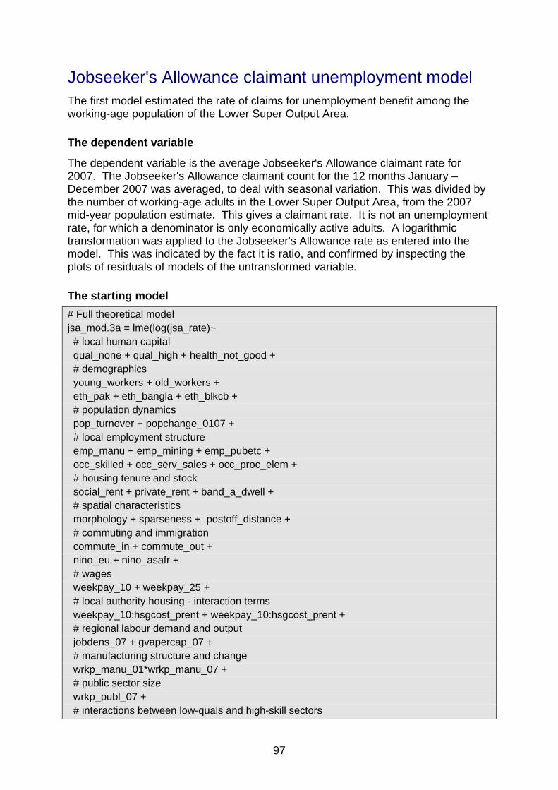
97

Jobseeker's Allowance claimant unemployment model The first model estimated the rate of claims for unemployment benefit among the working-age population of the Lower Super Output Area.

The dependent variable

The dependent variable is the average Jobseeker's Allowance claimant rate for 2007. The Jobseeker's Allowance claimant count for the 12 months January – December 2007 was averaged, to deal with seasonal variation. This was divided by the number of working-age adults in the Lower Super Output Area, from the 2007 mid-year population estimate. This gives a claimant rate. It is not an unemployment rate, for which a denominator is only economically active adults. A logarithmic transformation was applied to the Jobseeker's Allowance rate as entered into the model. This was indicated by the fact it is ratio, and confirmed by inspecting the plots of residuals of models of the untransformed variable.

The starting model # Full theoretical model jsa_mod.3a = lme(log(jsa_rate)~ # local human capital qual_none + qual_high + health_not_good + # demographics young_workers + old_workers + eth_pak + eth_bangla + eth_blkcb + # population dynamics pop_turnover + popchange_0107 + # local employment structure emp_manu + emp_mining + emp_pubetc + occ_skilled + occ_serv_sales + occ_proc_elem + # housing tenure and stock social_rent + private_rent + band_a_dwell + # spatial characteristics morphology + sparseness + postoff_distance + # commuting and immigration commute_in + commute_out + nino_eu + nino_asafr + # wages weekpay_10 + weekpay_25 + # local authority housing - interaction terms weekpay_10:hsgcost_prent + weekpay_10:hsgcost_prent + # regional labour demand and output jobdens_07 + gvapercap_07 + # manufacturing structure and change wrkp_manu_01*wrkp_manu_07 + # public sector size wrkp_publ_07 + # interactions between low-quals and high-skill sectors

98

wrkp_realest_07:qual_none + wrkp_finance_07:qual_none + # enterprise busi_startrate_07, random=~1|nuts3/la, data=high_lsoa)

Final model parameters

Variable Spatial level

Standard coefficient

% with no qualifications LSOA 0.068

% with highest level qualifications LSOA -0.066

% with health “not good” LSOA -0.041

% working-age residents aged <30 LSOA 0.129

% working-age residents aged >45 LSOA -0.195

% Pakistani ethnicity LSOA 0.088

% Bangladeshi ethnicity LSOA 0.049

% Black Caribbean ethnicity LSOA 0.166

Population turnover MSOA 0.133

% employed in manufacturing LSOA -0.040

% employed in public sector LSOA -0.023

“Urban type” (relative to Towns) LSOA 0.107

“Village type” (relative to Towns) LSOA -0.372

% in service/sales occupations LSOA -0.023

% in process/elementary occupations LSOA 0.077

% social rented dwellings LSOA 0.469

% private rented dwellings LSOA 0.345

% dwellings in tax band “A” LSOA 0.176

10th percentile of weekly average pay LA -0.081

Job density NUTS3 -0.521

GVA per capita NUTS3 0.607

Trend in manufacturing workplaces NUTS3 -0.088

N’hood % social rented tenure in area with high private rents relative to wages

LSOA/ LA

-0.122

N’hood % no qualifications in area with many real-estate and business services workplaces

LSOA/ NUTS3

-0.092

(Intercept) LSOA -0.182

99

Incapacity Benefit claimant level model This model estimated the ‘excess’ rate of Incapacity Benefit claims in the Lower Super Output Area. While some of this will reflect real differences in organic health by class, deprivation and so on, it is taken that some reflects labour market disadvantage (lack of jobs, weak incentives to return to economic activity, etc).

The dependent variable

The dependent variable is the ratio of actual Incapacity Benefit claims in 2007 to the expected number of claims in the Lower Super Output Area. The actual claims are the average of the Lower Super Output Area figures for the four quarters of 2007. An expected claimant count was calculated for each Lower Super Output Area by first calculating the England-wide rates of Incapacity Benefit claims for six age/sex groups (male and female, under 30, 30-45 and 45-pensionable age):

Claims aged 16-30 aged 30-44* aged 45-pens Male 154,420 345,337.5 748,153

Female 121,897.5 269,125 498,095

Population Male 4,853,800 5,532,600 6,239,500

Female 4,659,300 5,569,900 4,936,600

Rates Male 3.2% 6.2% 12.0%

Female 2.6% 4.8% 10.1%

*Incapacity Benefit claims for England are supplied for age band 25-35; the totals for this group were split between ‘age under 30’ and ‘age 30-44’ to align with the Small Area Population Estimates population age bands

These rates were then applied to the population numbers in each age/sex group at Lower Super Output Area level, from the Small Area Population Estimates, and then the predictions by age group summed to give a whole-Lower Super Output Area expected count.

The Incapacity Benefit actual/predicted ratio was entered untransformed into the model used for clustering. Later diagnostics suggested that the model would benefit from applying a logarithmic transformation; however, doing this does not materially change the parameter estimates from those shown below.

100

The starting model ibmod.3a = lme(ib_index~ # health health_not_good + # housing tenure social_rent + private_rent + # human capital qual_none + qual_high + # employment sectors emp_mining + emp_manu + emp_constr + emp_pubetc + # occupations occ_skilled + occ_proc_elem + # ethnicity eth_bangla + eth_pak + eth_blkcb + # demographics young_workers + old_workers + popchange_0107 + pop_turnover + # physical / housing dwellchange_0107 + postoff_distance + band_a_dwell + sparseness + morphology + # commuting commute_in + commute_out + # pay weekpay_10 + weekpay_25 + # housing costs/pay weekpay_25:hsgcost_prent + weekpay_25:hsgcost_social + weekpay_25:hsgcost_ownocc + # migraition nino_eu + nino_asafr + # historical and current job density, and consistent high/low jobdens_01*jobdens_07 + # past and present output, and consistent high/low gvapercap_01*gvapercap_07 + # workplace composition, past / present wrkp_manu_01*wrkp_manu_07 + wrkp_publ_01*wrkp_publ_07 + busi_startrate_01 + busi_startrate_07, random=~1|nuts3/la, data=high_lsoa)

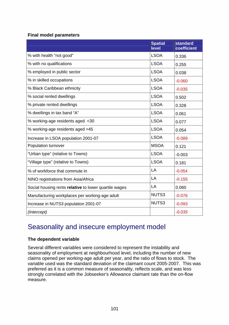
101

Final model parameters

Spatial level

standard coefficient

% with health “not good” LSOA 0.336

% with no qualifications LSOA 0.255

% employed in public sector LSOA 0.038

% in skilled occupations LSOA -0.060

% Black Caribbean ethnicity LSOA -0.035

% social rented dwellings LSOA 0.502

% private rented dwellings LSOA 0.328

% dwellings in tax band “A” LSOA 0.061

% working-age residents aged <30 LSOA 0.077

% working-age residents aged >45 LSOA 0.054

Increase in LSOA population 2001-07 LSOA -0.089

Population turnover MSOA 0.121

“Urban type” (relative to Towns) LSOA -0.003

“Village type” (relative to Towns) LSOA 0.181

% of workforce that commute in LA -0.054

NINO registrations from Asia/Africa LA -0.155

Social housing rents relative to lower quartile wages LA 0.060

Manufacturing workplaces per working-age adult NUTS3 -0.076

Increase in NUTS3 population 2001-07 NUTS3 -0.093

(Intercept) -0.035

Seasonality and insecure employment model

The dependent variable

Several different variables were considered to represent the instability and seasonality of employment at neighbourhood level, including the number of new claims opened per working-age adult per year, and the ratio of flows to stock. The variable used was the standard deviation of the claimant count 2005-2007. This was preferred as it is a common measure of seasonality, reflects scale, and was less strongly correlated with the Jobseeker's Allowance claimant rate than the on-flow measure.

102

The starting model casmod.3a = lme(jsa_stdev~ # underlying rate of new claims - v impt jsa_flowrate + # housing tenure social_rent + private_rent + # human capital qual_none + qual_high + # casualised / seasonal sectors emp_agri + emp_manu + emp_constr + emp_hotrest + emp_retail + # lower occupational class occ_skilled + occ_serv_sales + occ_proc_elem + # ethnicity eth_bangla + eth_pak + eth_blkcb + # age demographics young_workers + old_workers + # population dynamics dwellchange_0107 + popchange_0107 + pop_turnover + # sparse / distant postoff_distance + sparseness + morphology + # cheap housing band_a_dwell + # dormitory areas commute_in + commute_out + # low pay characteristic? weekpay_10 + weekpay_25 + # interaction term? hsgcost_social:weekpay_25 + hsgcost_prent:weekpay_25 + # associated with flexible migrant labour? nino_eu + nino_asafr + # low value / competition for labour jobdens_07 + gvapercap_07 + # seasonal sectors? wrkp_manu_07 + wrkp_hotrest_07 + wrkp_agri_07 + # startups busi_startrate_07, random=~1|nuts3/la, data=high_lsoa)

103

Final model parameters

Spatial level

standard coefficient

JSA on-flows per working-age adult LSOA 0.556

% social rented dwellings LSOA 0.048

% private rented dwellings LSOA 0.064

% dwellings in tax band “A” LSOA 0.063

% with no qualifications LSOA 0.097

% employed in agriculture LSOA -0.030

% employed in hotels/restaurants LSOA 0.084

% in service/sales occupations LSOA -0.026

% Bangladeshi ethnicity LSOA -0.101

% Pakistani ethnicity LSOA -0.064

% working-age residents aged <30 LSOA 0.051

% working-age residents aged >45 MSOA 0.258

Increase in LSOA population 2001-07 LSOA 0.124

Population turnover MSOA 0.054

NINO registrations from Asia/Africa LA 0.069

Private rents relative to lower quartile wages LA 0.088

Job Density 2007 LA 0.044

(Intercept) 0.011

Creating clusters The models were created by clustering against a new dataset. The copy dataset is created by, for each case (Lower Super Output Area), taking the standardised value of each predictor from each model, and multiplying it by the absolute value of the standard coefficient. Where a parameter appears in both models, the value is repeated. The group mean (NUTS3 random effect) for each model is also added as a variable to each case. This will tend to group Lower Super Output Areas from areas with high and low base rates of Jobseeker's Allowance and Incapacity Benefit together. The dependent variables (Incapacity Benefit and Jobseeker's Allowance) were not themselves included in the clusters, as they were assumed to be redundant given their known correlation with the model variables.

104

Choice of cluster amounts A scree plot (below) showing the sum of differences within groups for a range of different clusters was plotted, but did not show any clear break point. The choice of number of clusters was decided on the basis of possible policy applications, and to solicit comment on this issue from policy users.

Cluster algorithm

The k-means algorithm was run repeatedly to identify a stable set of clusters. Another choice would have been to specify a formal criterion (for example, maximum between-group difference, or minimum within-group difference), and used this criterion to decide automatically among many runs of the algorithm.

105

Annex D: Technical details of development of the nearest neighbour model for local authority performance Tools The calculation of neighbours and the testing of different neighbour models by sum of square differences was done using Microsoft Excel. This allowed the component variables of the nearest neighbour model to be changed interactively.

Variable standardisation for neighbour model Each authority’s value for each variable was standardised to its z-score, to reflect its deviation from the mean for that variable, relative to the extent of variation for all authorities. Standardisation transforms all variables into comparable scores that are indifferent to the original units of measurement and absolute range of values. Other standardisation methods are available; see Annex C.

Calculation of distance This distances between authorities were calculated by Euclidean distance. This is the square root of the sum of the squared differences on each variable in the neighbour model. So, the total distance between two authorities x and y, on variables a, b, and c would be calculated as follows:

2 2 2( ) ( ) ( )x y x y x ya a b b c c− + − + −

The greater the distance, the less similar the authorities. Note that there other means of calculating statistical distances, such as cosine similarity.

All the variables in the two bespoke neighbour models had equal weight, since there was no theoretical logic to do otherwise. Weightings could be applied at this stage. For example, feedback from local authorities might suggest that they consider ethnic diversity to be by far the most important challenge in building community cohesion. In this case, the distance on that variable could be given twice the weight (multiplied by two) before summing it with the other variables.