userâ€™s manual for the nati onal water-quality assessment program

U.S. GEOLOGICAL SURVEY

Open-File Report 03–172

User’s Manual for the National Water-Quality Assessment Program Invertebrate Data Analysis System (IDAS) Software: Version 3

NATIONAL WATER-QUALITY ASSESSMENT PROGRAM

By Thomas F. Cuffney

Raleigh, North Carolina2003

U.S. DEPARTMENT OF THE INTERIORGALE A. NORTON, Secretary

U.S. GEOLOGICAL SURVEY

CHARLES G. GROAT, Director

For additional information write to: Copies of this report can be purchased from:

District Chief U.S. Geological Survey U.S. Geological Survey Branch of Information Services 3916 Sunset Ridge Road Box 25286, Federal Center Raleigh, NC 27607 Denver, CO 80225

[email protected] 1-888-ASK-USGS

Information regarding the National Water-Quality Assessment (NAWQA) Program is available on the Internet at http://water.usgs.gov/nawqa/

Cover photograph: Opening screen of the Invertebrate Data Analysis System program.

The use of firm, trade, and brand names in this report is for identification purposes only and does not constitute endorsement by the U.S. Government.

FOREWORD

Foreword III

The U.S. Geological Survey (USGS) is committed to serve the Nation with accurate and timely scientific information that helps enhance and protect the overall quality of life and that facilitates effective management of water, biological, energy, and mineral resources (http://www.usgs.gov/). Information on the quality of the Nation’s water resources is of critical interest to USGS because it is so integrally linked to the long-term availability of water that is clean and safe for drinking and recreation and that is suitable for industry, irrigation, and habitat for fish and wildlife. Escalating population growth and increasing demands for multiple water uses make water availability, now measured in terms of quantity and quality, even more critical to the long-term sustainability of our communities and ecosystems.

The USGS implemented the National Water-Quality Assessment (NAWQA) Program to support national, regional, and local information needs and decisions related to water-quality management and policy (http://water.usgs.gov/nawqa/). Shaped by and coordinated with ongoing efforts of other Federal, State, and local agencies, the NAWQA Program is designed to answer: What is the condition of our Nation’s streams and ground water? How are the conditions changing over time? How do natural features and human activities affect the quality of streams and ground water, and where are those effects most pronounced? By combining information on water chemistry, physical characteristics, stream habitat, and aquatic life, the NAWQA Program aims to provide science-based insights for current and emerging water issues and priorities. NAWQA results can contribute to informed decisions that result in practical and effective water-resource management strategies that protect and restore water quality.

Since 1991, the NAWQA Program has implemented interdisciplinary assessments in more than 50 of the Nation’s most important river basins and aquifer systems, referred to as Study Units (http://water.usgs.gov/nawqa/studyu.html). Collectively, these Study Units account for more than 60 percent of the overall water use and population served by public water supply, and are representative of the Nation’s major hydrologic landscapes, priority ecological resources, and agricultural, urban, and natural sources of contamination.

Each assessment is guided by a nationally consistent study design and methods of sampling and analysis. The assessments thereby build local knowledge about water-quality issues and trends in a particular

stream or aquifer while providing an understanding of how and why water quality varies regionally and nationally. The consistent, multi-scale approach helps to determine if certain types of water-quality issues are isolated or pervasive, and allows direct comparisons of how human activities and natural processes affect water quality and ecological health in the Nation’s diverse geographic and environmental settings. Comprehensive assessments on pesticides, nutrients, volatile organic compounds, trace metals, and aquatic ecology are developed at the national scale through comparative analysis of the Study-Unit findings (http://water.usgs.gov/nawqa/natsyn.html).

The USGS places high value on the communication and dissemination of credible, timely, and relevant science so that the most recent and available knowledge about water resources can be applied in management and policy decisions. We hope this NAWQA publication will provide you the needed insights and information to meet your needs, and thereby foster increased awareness and involvement in the protection and restoration of our Nation’s waters.

The NAWQA Program recognizes that a national assessment by a single program cannot address all water-resource issues of interest. External coordination at all levels is critical for a fully integrated understanding of watersheds and for cost-effective management, regulation, and conservation of our Nation’s water resources. The Program, therefore, depends extensively on the advice, cooperation, and information from other Federal, State, interstate, Tribal, and local agencies, nongovernment organizations, industry, academia, and other stakeholder groups. The assistance and suggestions of all are greatly appreciated.

Robert M. HirschAssociate Director for Water

http://www.usgs.gov/

http://water.usgs.gov/nawqa

http://water.usgs.gov/nawqa/studyu.html

CONTENTS
Abstract ................................................................................................................................................................................. 1Introduction ........................................................................................................................................................................... 1
Purpose and scope ....................................................................................................................................................... 2Acknowledgments ....................................................................................................................................................... 2

Invertebrate Data Analysis System (IDAS)........................................................................................................................... 2Capabilities.................................................................................................................................................................. 2Sources of data used by IDAS..................................................................................................................................... 3Characteristics of Bio-TDB data ................................................................................................................................. 4

Provisional and conditional identifications ....................................................................................................... 4Ambiguous taxa ................................................................................................................................................ 5

Installation................................................................................................................................................................... 6System requirements ......................................................................................................................................... 6Installing the IDAS software............................................................................................................................. 6Updates.............................................................................................................................................................. 7

Help and documentation ............................................................................................................................................. 7Using IDAS ........................................................................................................................................................................... 8

Starting IDAS.............................................................................................................................................................. 8Common features of modules ..................................................................................................................................... 8

Menu items........................................................................................................................................................ 8Status bars ......................................................................................................................................................... 9Loading data...................................................................................................................................................... 9Resetting or exiting a module............................................................................................................................ 11

Edit Data module................................................................................................................................................................... 12Subset data .................................................................................................................................................................. 12

Sample information........................................................................................................................................... 13Taxonomy.......................................................................................................................................................... 14

Combine/delete data.................................................................................................................................................... 15Summarize taxa ........................................................................................................................................................... 16

Data Preparation module....................................................................................................................................................... 17Processing options....................................................................................................................................................... 18

Select sample type(s) to process ....................................................................................................................... 19Calculate densities............................................................................................................................................. 21Data deletions based on NWQL BG processing notes...................................................................................... 21Data deletions based on lifestages..................................................................................................................... 22Options based on combining lifestages............................................................................................................. 22Options for forming qualitative (QUAL) samples ............................................................................................ 24Select lowest taxonomic level ........................................................................................................................... 24Delete rare taxa ................................................................................................................................................. 25Options for resolving ambiguities ..................................................................................................................... 31

Sample-by-sample basis .......................................................................................................................... 33Option 1 (RS1): Delete ambiguous parents and retain children ................................................... 34Option 2 (RS2): Delete children of ambiguous parents and add their abundances

to the abundance of the ambiguous parent ...................................................................... 35Option 3 (RS3): If the abundance of an ambiguous parent is greater than the sum

of the abundances of the children, add the children’s abundances to that of the parent and delete the children; otherwise, retain the children and delete the parent........................................................................................................ 37

Option 4 (RS4): Distribute ambiguous parent abundance among children in accordance with the relative abundance of each child .................................................... 39

Option 5 (RS5): None — retain ambiguous taxa ........................................................................... 41

Contents V

Combined samples................................................................................................................................... 42Option 1 (RC1): Delete ambiguous parents and retain children.................................................... 42Option 2 (RC2): Delete children of ambiguous parents and add their abundances

to the abundance of the ambiguous parent ...................................................................... 43Option 3 (RC3): If an ambiguous parent’s abundance is greater than the sum

of the children’s abundances, add the children’s abundances to the parent and delete the children. Otherwise, retain the children and delete the parent ................. 44

Option 4 (RC4): Distribute ambiguous parent abundance among children in accordance with the relative abundance of each child................................................. 45

Option 5 (RC5): None — retain ambiguous taxa ........................................................................... 46Associating ambiguous children with ambiguous parents ............................................................ 46

Running the Data Preparation module......................................................................................................................... 53Output from the Data Preparation module................................................................................................................... 54Resetting or exiting the module ................................................................................................................................... 55

Calculate Community Metrics module.................................................................................................................................. 55Processing options ....................................................................................................................................................... 56Updating attributes file ................................................................................................................................................ 58Output from the module............................................................................................................................................... 59Resetting or exiting the module ................................................................................................................................... 59

Calculate Diversities and Similarities module....................................................................................................................... 59Processing options ....................................................................................................................................................... 60Output from the module............................................................................................................................................... 61Resetting or exiting the module ................................................................................................................................... 61

Data Export module............................................................................................................................................................... 61Processing options ....................................................................................................................................................... 62Duplicate sort codes..................................................................................................................................................... 64Resetting or exiting the module ................................................................................................................................... 64

Troubleshooting ..................................................................................................................................................................... 64Types of errors ............................................................................................................................................................. 64Error messages............................................................................................................................................................. 65Reporting program bugs .............................................................................................................................................. 65Abnormal termination of IDAS ................................................................................................................................... 66

Summary................................................................................................................................................................................ 66References cited..................................................................................................................................................................... 67Appendix I: Bio-TDB data file formats................................................................................................................................. 70Appendix II: Data output formats produced by the Data Preparation module ...................................................................... 73Appendix III: Data output formats produced by the Calculate Community Metrics module ............................................... 78Appendix IV: Data output formats produced by the Calculate Diversities and Similarities module .................................... 83Appendix V: Data output formats produced by the Data Export module.............................................................................. 93Appendix VI: Error messages................................................................................................................................................ 98

FIGURES

1. Opening screen of the IDAS program showing the buttons that activate the five program modules....................... 92. A 5-panel status bar displays information at the bottom of each module window .................................................. 103. File-selection window displayed by IDAS modules for opening data files ............................................................. 104. Standard window displayed by IDAS for selecting an Excel spreadsheet or Access data table .............................. 115. The IDAS program warns the user if executing the module will produce a spreadsheet or data table

name that already exists in the Excel workbook or Access database. ..................................................................... 116. The opening screen of the Edit Data module ........................................................................................................... 127. File-type selection window used in the Edit Data module ....................................................................................... 138. Selection window used to subset data based on sample information....................................................................... 139. Form used to enter a data table or spreadsheet name to store data........................................................................... 14

10. Selection window used to subset data based on taxonomic information ................................................................. 1511. Selection window used to select data tables or spreadsheets to combine ................................................................ 16

VI Contents

12. The distribution of taxa can be summarized based on BU_ID or the combination of BU_ID and lifestage ........... 1713. Main window of the Data Preparation module with the processing options displayed ........................................... 1914. Form for selecting the range of dates over which to aggregate RTH, DTH, and QMH samples

when creating the QUAL sample ............................................................................................................................. 2015. Data entry screen for selecting RTH and(or) DTH samples to pair with a QMH

sample in the formation of a QUAL sample ............................................................................................................ 2016. The method selected to resolve ambiguous taxa can have a profound effect

on taxa richness and abundance ............................................................................................................................... 3417. Pop-up window that prompts the user to select an upper taxonomic limit for the aggregation

of data when using ambiguous taxa resolution method 2 (RS2, RC2) .................................................................... 3618. Error message generated when the upper taxa limit for resolving ambiguities is lower than the level

chosen as the lowest taxonomic level....................................................................................................................... 3719. The IDAS program informs the user of the number of ambiguous taxa that need to be resolved

through user intervention ......................................................................................................................................... 4720. The IDAS program allows the user to select children to match with ambiguous parents when

it encounters a sample that contains an ambiguous parent but no associated children............................................ 4821. This message box can be used to manually change the percentage of parent abundance

that is assigned to a child ......................................................................................................................................... 4922. The processing status window from the Data Preparation module .......................................................................... 5423. Main window of the Calculate Community Metrics module ................................................................................... 5624. The IDAS program allows the user to determine how to match Bio-TDB taxa names to those used

by the U.S. Environmental Protection Agency ........................................................................................................ 5825. The IDAS program warns the user if it cannot match Bio-TDB taxonomic names with those used

by the U.S. Environmental Protection Agency and displays a list of names that cannot be matched ..................... 5826. Main window of the Calculate Diversities and Similarities module ........................................................................ 6027. Main window of the Export Data module ................................................................................................................ 6228. The IDAS program prompts the user to supply a header line for files stored in CANOCO

native format files..................................................................................................................................................... 6329. The IDAS message box that alerts the user of the presence of duplicate sort codes in the data .............................. 6430. Error message generated by an anticipated and trappable error ............................................................................... 6531. Error message generated by an unanticipated but trappable error............................................................................ 65

TABLES

1. Structure of the “_Invert_Results_Comb.xls” file exported from Bio-TDB in a 20-column format ....................... 42. Example of multiple entries for one taxon associated with a single sample ............................................................ 43. Conditional and provisional identifications confined to the BU_ID column of the Bio-TDB export file ............... 54. Example of ambiguous taxa ..................................................................................................................................... 65. National Water Quality Laboratory Biological Group (NWQL BG) standardized sample-processing

notes that are recognized by the IDAS program ...................................................................................................... 216. The three options for applying NWQL BG sample-processing notes operate differently

if ambiguous taxa are present................................................................................................................................... 227. Examples of how the IDAS program can modify data using sample-processing notes (Notes)

and lifestage data...................................................................................................................................................... 238. An example of how the “Select lowest taxonomic level” option operates at the species,

genus, family, and order levels ................................................................................................................................. 249. Effects of “delete rare taxa” options 1 – 4 on taxa richness and density ................................................................... 26

10. Hypothetical density data used to illustrate how the options for deleting rare taxa determine which taxa to delete.................................................................................................................................................. 27

11. Examples of the steps used to delete rare taxa in option 1 as applied to the data in table 10 .................................. 2812. Examples of the steps used to delete rare taxa in option 2 as applied to the data in table 10 .................................. 2913. Examples of the steps used to delete rare taxa in option 3 as applied to the data in table 10 .................................. 3014. Examples of the steps used to delete rare taxa in option 4 as applied to the data in table 10 .................................. 3115. Hypothetical invertebrate data used to illustrate the eight methods for resolving ambiguous taxa ......................... 3316. Taxa richness and abundance obtained by using different methods for resolving taxonomic ambiguities.............. 34

Contents VII

17. Results obtained by using processing method RS1 (deleting ambiguous parents and retaining children separately for each sample) to resolve ambiguous taxa in table 15 ........................................................... 35

18. Results obtained by using processing method RS2 (deleting children of ambiguous parents and adding their abundances to that of the parents) to resolve ambiguous taxa in table 15 .................................... 36

19. Results obtained by specifying different upper taxa limits in the RS2 processing method ..................................... 3720. An example of how processing method RS3 resolves ambiguous taxa over three iterations from

genus to family......................................................................................................................................................... 3821. Results obtained by using processing method RS3 to resolve ambiguous taxa in table 15 ..................................... 3922. Examples of how processing method RS4 distributes the abundances of ambiguous parents

among ambiguous children for sample 7896 in table 15 ......................................................................................... 4023. Results obtained by using processing method RS4 (distributing the abundance of ambiguous

parents among their children in accordance with the relative abundance of each child) to resolve ambiguous taxa in table 15....................................................................................................................................... 41

24. Results obtained by using processing method RC1 (delete ambiguous parents and retain children) to resolve ambiguous taxa in table 15 ...................................................................................................................... 43

25. Results obtained by using processing method RC2 (deleting children of ambiguous parents and adding their abundances to the abundance of the parents) to resolve ambiguous taxa in table 15 ................... 44

26. Example of how processing method RC3 resolves ambiguous taxa when parents or children are not present in the sample.................................................................................................................................... 45

27. Results obtained by using processing method RC3 to resolve ambiguous taxa in table 15..................................... 4528. Results obtained by using processing method RC4 (distributing the abundance of ambiguous

parents among their children) to resolve ambiguous taxa in table 15...................................................................... 4629. Effects of distributing, deleting, or retaining parents when processing ambiguous taxa by using

processing method RC1 ........................................................................................................................................... 5030. Effects of distributing, deleting, or retaining parents when processing ambiguous taxa by using

processing method RC4 ........................................................................................................................................... 5231. Output tables that can be produced by the Calculate Community Metrics module ................................................. 59

VIII Contents

CONVERSION FACTORS and TEMPERATURE

Temperature: Temperature is given in degrees Celsius (°C), which can be converted to degrees Fahrenheit (°F) as follows:

°F = (1.8 × °C) + 32

Multiply By To obtain

Lengthmicrometer (µm) 0.00003937 inch (in.)millimeter (mm) 0.03937 inch (in.)centimeter (cm) 0.3937 inch (in.)

meter (m) 3.281 foot (ft)kilometer (km) 0.6214 mile (mi)

Areasquare centimeter (cm2) 0.155 square inch (in2)

square meter (m2) 10.76 square foot (ft2)square kilometer (km2) 0.3861 square mile (mi2)

Volumeliter (L) 1.057 quart (qt)liter (L) 0.2642 gallon (gal)

milliliter (mL) 0.0338 ounce, fluid (oz)

Flowcentimeter per second (cm/s) 0.0328 foot per second (ft/s)

Massgram (g) 0.03527 ounce, avoirdupois (oz)

Pressurekilopascal (kPa) 0.1450 pound-force per square inch (lbf/in2)

ABBREVIATIONS FREQUENTLY USED IN THIS REPORT

A adult lifestage P pupal lifestage

ALBE Albemarle-Pamlico Drainage Basin QMH qualitative multi-habitat

ALMN Allegheny and Monongahela Drainage Basin QUAL qualitative sample: RTH+DTH+QMH

Ambig ambiguous taxon RAM random access memory

BG Biological Group of the NWQL RBP Rapid Bioassessment Protocol

Bio-TDB Biological Transactional Database RTH richest-targeted habitat

BU_ID organism name applied by BG SampleID sample identifier used by Bio-TDB

DTH depositional-targeted habitat SortCode taxonomic sort code

IDAS Invertebrate Data Analysis System SMCOD sample identification code

imm. immature sp. species

indet. indeterminate STAID station identifier

KB kilobyte SUID 4-character Study Unit identifier

L larval lifestage TOL tolerance value

MB megabyte USEPA U.S. Environmental Protection Agency

MHz megahertz YAKI Yakima River Basin

no. number % percentage

NAWQA National Water-Quality Assessment ≤ less than or equal to

NWQL National Water Quality Laboratory ± plus or minus

Contents IX

GLOSSARY

Abundance — The number of organisms in a sample, either for the whole sample or for each taxon.

Access tables — Rows and columns of data that form the basic data storage units in Microsoft Access® database files.

Ambiguous child — A taxon that occurs at a lower taxonomic level within a group of ambiguous taxa. For example, in a sample that contained data for Hydropsychidae, Hydropsyche, and Hydropsyche sparna; Hydropsyche would be the ambiguous child of the ambiguous parent Hydropsychidae and Hydropsyche sparna would be the ambiguous child of the ambiguous parents Hydropsychidae and Hydropsyche.

Ambiguous parent — A taxon within a group of ambiguous taxa that occurs at a higher taxonomic level than do other taxa within the group. For example, in a sample that contained data for Hydropsychidae, Hydropsyche, and Hydropsyche sparna; both Hydropsychidae and Hydropsyche would be ambiguous parents of Hydropsyche sparna, and Hydropsychidae would be an ambiguous parent of Hydropsyche.

Ambiguous taxon — A taxon in a data set for which data are reported at one or more lower or higher taxonomic levels within the taxonomic hierarchy. For example, in a sample that contained data for Hydropsychidae, Hydropsyche, and Hydropsyche sparna; all three taxa would be considered ambiguous.

AreaSampTot — The name of the column that stores the total area sampled (cm2) during the collection of quantitative samples (RTH and DTH).

Benthic — Refers to bottom; for example, benthic organisms that live on or burrow into an aquatic substrate.

Biological Data Analysis System (BDAS) — A USGS software package for the analysis of NAWQA Program ecological data that was developed for use on the Data General computer system.

Biological Transactional Database (Bio-TDB) — The database used to store biological data collected by the NAWQA Program.

BU_ID — The taxonomic name provided by the Biological Group at the USGS’s National Water Quality Laboratory. BU_ID’s may include conditional or provisional identifications.

CANOCO — A commercially available multivariate statistical package for the analysis of community data.

Child — See ambiguous child.Collection date (CollectionDate) — The date on which a

sample was collected.Community metrics — A numerical summarization of the

characteristics of a community.Component — See sample component.

Conditional identification — An organism that has been assigned to a taxon that it closely resembles, but for which it does not fully meet the published description. These identifications are approximations rather than definitive.

Cornel Ecology Package (CEP) — A statistical package developed in the 1970’s for the multivariate analysis of community data.

Data set — A group of samples that are contained within an Excel spreadsheet or Access data table.

Data table — See Access tables.Density — The number of organisms in a sample divided by

the area sampled in square meters (m2). Expressed as density for the whole sample, taxon, or group of taxa.

Depositional-targeted habitat (DTH) — A habitat within the sampling reach where fine sediments (for example, sand and silt) are deposited. A composite sample from this habitat is referred to as a “DTH sample.”

Dissimilarity index — An index that measures how different two samples are based on the kinds of taxa present in the samples and(or) their abundances. Dissimilarity indices are related to similarity indices.

Diversity index — An index that reduces the structure of a community to a numeric value by mathematically describing how abundance is distributed among taxa in a sample. Diversity indices are related to dominance and evenness indices.

Dominance index — A numeric index that measures how strongly community structure is dominated by numerically abundant taxa. Dominance indices are related to diversity and evenness indices.

Ecological tolerance — A numeric value assigned to a taxon that indicates how well the taxon tolerates pollution. Low values indicate intolerant taxa that will disappear quickly from communities as water quality degrades. High values indicate tolerant taxa that will remain in the community as water quality degrades.

Evenness index — A numeric index that measures how uniformly (evenly) abundance is distributed among taxa in a sample. Evenness indices are related to dominance and diversity indices.

Functional feeding group — A group of taxa that have similar adaptations for feeding.

Functional group — See functional feeding group. Higher taxonomic level — A position in the taxonomic

hierarchy that is closer to the level of phylum than the level against which it is being compared. In IDAS the highest taxonomic level is phylum, the lowest level is species.

Invertebrates — Animals that do not have backbones, such as worms, clams, crustaceans, and insects.

X Glossary

Lab notes — Notes made by the NWQL BG during sample processing that document why organisms were not identified to taxonomic levels specified in the sample processing protocol.

Laboratory notes — See lab notes.Lifestage — One of four stages (egg, larva, pupa, and adult)

in the development of insects.Lower taxonomic level — A position in the taxonomic

hierarchy that is closer to the level of species than the level against which it is being compared. In IDAS, the highest taxonomic level is phylum and the lowest level is species.

Lowest taxonomic level — The lowest level of the taxonomic hierarchy that will be used for an analysis. Data in levels below this level will be aggregated up to this taxonomic level. In IDAS, the highest taxonomic level is phylum and the lowest level is species.

Metrics — See community metrics.Module — A set of related analyses in IDAS.MVSP — A commercially available multivariate statistical

package for the analysis of community data.Notes — See lab notes.NWQL BG — National Water Quality Laboratory Biological

Group. This group is responsible for processing (picking, identifying, and counting) NAWQA invertebrate samples.

Parent — See ambiguous parent.PC-ORD — A commercially available multivariate statistical

package for the analysis of community data.Phylogenetic order — The taxonomic hierarchy

arranged along inferred lines of descent based on paleontological, morphological, or other evidence.

Proportion — The number or density of organisms of a particular taxon present in a sample divided by the total abundance or density in that sample. Proportions vary between 0 and 1.

Proportional abundance — The number of organisms of a particular taxon present in a sample divided by the total number of organisms in that sample. Proportional abundance varies between 0 and 1.

Proportional density — The density of organisms of a particular taxon present in a sample divided by the total density of organisms in that sample. Proportional density varies between 0 and 1.

Provisional identification — An organism that has been assigned to a provisional taxon reported in the literature, but the specific identify remains unknown (Hydropsyche sp. A). Also known as “operational taxonomic units” or “OTUs.” These identifications are approximations rather than definitive.

Qualitative multihabitat (QMH) — A series of different habitats identified in a reach from which discrete collections of invertebrates are taken and later combined to form a composite sample. The composite sample is referred to as a “QMH sample.”

Qualitative sample (QUAL) — A list of taxa found at a site that is formed by combining data from QMH samples with data from RTH and(or) DTH samples collected over a specified range of sampling dates.

Rare taxa — Taxa that occur at only a few sites or that contribute only a small fraction of the total abundance in a sample.

Reach — A length of stream (150 – 300 m for wadeable streams; 300 – 1,000 m for nonwadeable streams) that is chosen to represent a uniform set of physical, chemical, and biological conditions within a stream segment. It is the principal sampling unit for collecting physical, chemical, and biological data in the NAWQA Program.

Relative abundance — The number of organisms of a particular taxon present in a sample divided by the total number of organisms in that sample and multiplied by 100. Relative abundance varies between 0 and 100.

Relative density — The density of organisms of a particular taxon present in a sample divided by the total density of organisms in that sample and multiplied by 100. Relative density varies between 0 and 100.

Richest-targeted habitat (RTH) — A targeted habitat (usually a riffle or woody snag) in a reach where the taxonomically richest invertebrate community is theoretically located. Discrete collections of invertebrates are taken from this habitat and combined to form a composite sample. The composite sample is referred to as an “RTH sample.”

Richness — See taxa richness.Sample — Operationally defined as all of the material and

organisms collected during one application of the NAWQA Program sampling protocol for a particular sample type (for example, invertebrate RTH sample). A single sample may be subdivided during field processing to create multiple sample components.

Sample component — A subset of an invertebrate sample that is produced by processing a sample in the field. Field processing can produce up to four different sample components: large-rare, main-body, split, and elutriate.

Sample identification code (SMCOD) — A 16-character alphanumeric code that uniquely identifies each sample component.

Sample medium — The type of biological community being sampled (algae, invertebrates, or fish).

Glossary XI

SampleMediumCode — The name of the column that holds information on the sample medium.

Sample number — A 4-digit number that Bio-TDB uses to uniquely identify each sample component.

Sample type — A certain type of invertebrate sample collected in a reach from either a single targeted habitat (RTH or DTH) or multiple habitats (QMH).

SampleType — The name of the column that stores sample type information.

SAS — A commercially available statistics package.Similarity index — An index that measures how alike two

samples are based on the kinds of taxa present in the samples and(or) their abundances.

Sort Code (SortCode) — A number supplied by Bio-TDB that allows data to be sorted into phylogenetic order.

S-PLUS — A commercially available statistics package.Spreadsheet — A series of rows and columns that holds

information in Microsoft Excel® files.STAID — Station identification number.SUID — A 4-letter abbreviation used to identify Study Units.SYSTAT — A commercially available statistics package.Taxa — Plural of taxon.

Taxa richness — The number of different taxa in a sample.Taxon — A taxonomic group that is sufficiently distinct to be

worthy of being distinguished by name and ranked in a definite category of the taxonomic hierarchy.

Taxonomic hierarchy — A hierarchic classification scheme that orders taxa into related groups based on similarities in morphological structure. The highest level of the hierarchy (phylum) has the most general characteristics and the lowest level (species) the most specific characteristics and greatest morphological similarities among organisms.

Taxonomic level — A grouping in the taxonomic hierarchy.Tolerance — See ecological tolerance.TWINSPAN — Two-Way Indicator Species Analysis. A

computer software package for the multivariate analysis of community data that is part of the Cornel Ecology Package of software.

Visual Basic — A computer programming language for Microsoft Windows®.

Workbook — A collection of spreadsheets contained within one Microsoft Excel® file.

Zoogeography — The study of the geographic distribution of animals.

XII Glossary

User’s Manual for the National Water-Quality Assessment Program Invertebrate Data Analysis System (IDAS) Software: Version 3By Thomas F. Cuffney

ABSTRACT

The Invertebrate Data Analysis System (IDAS) software provides an accurate, consistent, and efficient mechanism for analyzing invertebrate data collected as part of the National Water-Quality Assessment Program and stored in the Biological Transactional Database (Bio-TDB). The IDAS software is a stand-alone program for personal computers that run Microsoft (MS) Windows®. It allows users to read data downloaded from Bio-TDB and stored either as MS Excel® or MS Access® files. The program consists of five modules. The Edit Data module allows the user to subset, combine, delete, and summarize community data. The Data Preparation module allows the user to select the type(s) of sample(s) to process, calculate densities, delete taxa based on laboratory processing notes, combine lifestages or keep them separate, select a lowest taxonomic level for analysis, delete rare taxa, and resolve taxonomic ambiguities. The Calculate Community Metrics module allows the user to calculate over 130 community metrics, including metrics based on organism tolerances and functional feeding groups. The Calculate Diversities and Similarities module allows the user to calculate nine diversity and eight similarity indices. The Data export module allows the user to export data to other software packages and produce tables of community data that can be imported into spreadsheet and word-processing programs. Though the IDAS program was developed to process invertebrate data downloaded from USGS databases, it will work with other data sets that are converted to the USGS (Bio-TDB) format. Consequently, the data manipulation, analysis, and export procedures provided by the IDAS program can be used by anyone involved in using benthic macroinvertebrates in applied or basic research.

INTRODUCTION

The U.S. Geological Survey’s (USGS) National Water-Quality Assessment (NAWQA) Program is a perennial program designed to provide a comprehensive, interdisciplinary water-quality assessment of the Nation’s flowing water resources (Hirsch and others, 1988; Leahy and others, 1990). During the first decade of the NAWQA Program’s operation (1991 – 2001), ecological studies were conducted to assess the occurrence and distribution of algal, invertebrate, and fish communities in about 51 Study Units (Gilliom and others, 1995). These Study Units represent the dominant hydrologic systems nationwide and are staggered in time with respect to implementation and high- and low-intensity sampling periods (Gilliom and others, 1995). During the second decade of the NAWQA Program (2001–2011), ecological studies are being conducted as part of nationally guided topical studies that address selected water-quality issues and as part of long-term-trends monitoring within the Study Units.

Accurate, consistent, and timely analyses of invertebrate data are critical when providing interpretations of water-quality conditions that integrate physical, chemical, and biological attributes of aquatic ecosystems at local, regional, and national scales. A common set of data-analysis tools facilitates integrated analyses by making communications among multiple scientific teams (for example, study unit, regional, and national) easier and more precise, and it provides a means of documenting and archiving data analyses. A common set of invertebrate data-analysis tools was not available during the first decade of the NAWQA Program, making it difficult to duplicate and archive data analyses conducted during this period. Adoption of a common set of self-documenting software tools makes data analysis, communication, and archiving results and analyses more

Abstract 1

accurate, efficient, and timely during the second decade of the NAWQA Program.

Purpose and Scope

The purpose of this report is to provide information on the use and capabilities of the Invertebrate Data Analysis System (IDAS) software. This User’s Manual explains how to acquire the software, load it onto a personal computer, and run the software. It discusses the relation between the NAWQA Program ecological database and the IDAS program, and provides instructions on how to use IDAS as a tool for exploring, analyzing, and exporting invertebrate data to other software programs. Though developed for processing invertebrate data downloaded from the NAWQA Program databases, the IDAS program will analyze any invertebrate data converted to the format specified in the User’s Manual. Consequently, this program will be of value to non-USGS scientists looking for an efficient means of processing invertebrate data. The IDAS software was designed to provide a rapid, consistent, and efficient means of analyzing data stored in the NAWQA Program’s Biological Transactional Database (Bio-TDB). The IDAS software was developed to help data analysts at the study-unit, regional, and national levels work either independently or in cooperation with one another, and it also facilitates the archiving of data analyses by providing procedures that automatically document the options used in the analyses. The IDAS software provides a set of standard, data-analysis procedures that are citable and that can be used by scientists within and outside of the USGS.

Acknowledgments

The IDAS software is a distillation of over 12 years of experience working with large quantities of invertebrate data in multiple databases and with numerous biologists associated with the NAWQA Program. Specifications for the software program originally were established from the input of NAWQA Program biologists during the development of the Biological Data Analysis System (BDAS) in 1994 – 95. I am indebted to the biologists who provided input at that time — Michael Bilger, Robert Black, Larry Brown, James Coles, Carol Couch, Charles Demas, Steven Frenzel, Jeffrey Frey, Robert Goldstein, Steven Goodbred, Martin Gurtz, Evan Hornig, Clifford Hupp, Terry Maret, Michael Meador, Bruce Moring, Mark Munn, Karen Murray, James Petersen, Stephen Porter, Stephen Rheaume, Peter Ruhl,

Barbara Scudder, Terry Short, Stephen Sorenson, Cathy Tate, Ian Waite, and Humbert Zappia. Several biologists provided input in the development of IDAS and assisted in helping to test the installation and operation of the IDAS software program — Humbert Zappia, James Coles, Ian Waite, Thomas Abrahamsen, Elise Giddings, Robert Ourso, Mitch Harris, Terry Maret, Dorene MacCoy, Karen Murray, and Jeffrey Powell. The Ecological Integration Project and the Albemarle-Pamlico Drainage and Yakima River Basin Study Units provided additional support for the development of this software.

INVERTEBRATE DATA ANALYSIS SYSTEM (IDAS)

The IDAS software package is a special purpose program written in Microsoft Visual Basic® 6.0. It is intended to provide NAWQA Program biologists with a flexible and efficient mechanism for analyzing invertebrate data downloaded from Bio-TDB and for preparing Bio-TDB data for use in other analytical programs, such as MVSP, CANOCO, SYSTAT, S-PLUS, and SAS. In general, the format of the invertebrate data supplied by Bio-TDB does not allow the user to analyze invertebrate data without making substantial modifications to the data files. The IDAS software program provides a quick and flexible means of manipulating and analyzing invertebrate data obtained from Bio-TDB data.

Capabilities

The IDAS program consists of five program modules that allow the user to manipulate data sets, calculate community metrics, and export data to other programs. These modules provide the following capabilities:

1. Edit Data module:

A. Subset data option is used to generate subsets of data based on sample information (for example, date, sample type, station) or taxo-nomic groupings (for example, order, family).

B. Combine data sets option can be used to combine

TIP: Use the Edit Data module to select subsets of data for analysis and to examine the distribution of taxa among sites. This will help guide decisions (for example, deleting rare taxa) that are required in the Data Preparation module.

2 User’s Manual for the National Water-Quality Assessment Program Invertebrate Data Analysis System (IDAS) Software: Version 3

one or more Excel spreadsheets or Access data tables of similar structure into a new Excel spreadsheet or Access table.

C. Delete data sets option is used to delete one or more Excel spreadsheets or Access tables.

D. Summarize taxa option can be used to identify ambiguities and provide distribution statistics for taxa in a data set.

2. Data Preparation module:

A. Select sample types (QMH, DTH, RTH, and(or) QUAL = QMH+RTH+DTH) to process.

B. Calculate densities, in number per square meter (no./m2), using the sample area information contained in the file “_Sample_All.xls” exported by Bio-TDB.

C. Delete data based on Biological Group (BG) processing notes, such as immature or damaged.

D. Delete pupae or non-aquatic adult insects.

E. Combine or retain information on lifestages.

F. Select how to form QUAL samples: QMH+RTH and(or) DTH.

G. Select the lowest taxonomic level (for example — family, tribe,genus) for the data set.

H. Delete rare taxa based on the percentage of total abundance in a sample and(or) the percentage of sites at which the taxa occur.

I. Resolve ambiguous taxa separately for each sample or for a combination of data by using one of five methods:a. Delete ambiguous parents and retain children.

b. Delete children of ambiguous parents and add their abundance to the parent taxa.

c. Retain children’s abundance if it is larger than parent abundance. Otherwise, combine children with parent taxa.

d. Distribute ambiguous parent abundance among children in accordance with the relative abundance of the children.

e. None — retain ambiguous taxa.3. Calculate Community Metrics module:

A. Richness metrics will calculate 25 richness and 24 percent-richness metrics.

B. Abundance metrics will calculate 25 abundance and 24 percent-abundance metrics.

C. Tolerance metrics will calculate average tolerance based on richness and abundance.

D. Functional group metrics will calculate 16 richness and 16 percent-abundance metrics.

4. Calculate Diversities and Similarities module:

A. Calculate 9 diversity, dominance, and evenness indices.

B. Calculate 8 similarity and dissimilarity indices.5. Data Export module:

A. Export data as abundance, density, proportions, or percentages.

B. Export data in comma-delimited ASCII format with rows as samples or taxa.

C. Export data in tab-delimited ASCII format with rows as taxa.

D. Export data in CANOCO-condensed format.

The Data preparation module reads data in the format exported by Bio-TDB (that is, combined results format, appendix table I-1). This module produces a new format (processed data, appendix table II-1) that is used by the other four modules (Edit Data, Calculate Community Metrics, Calculate Diversities and Similarities, and Data Export). The Edit Data module is the only module that can process data that are in the original Bio-TDB format (appendix table I-1) or the processed format (appendix table II-1). The other three modules can use data only in the processed format. All modules except for the Data Export module store data in the original files either as new spreadsheets (Excel) or new data tables (Access). The Data Export module writes data to ASCII text files rather than to Excel or Access files.

Sources of Data Used by IDAS

All analyses are based on the invertebrate abundance information contained in the combined results files exported from Bio-TDB (v. 2.2.0). These files are obtained from Bio-TDB by using the combined data export option (Data/SU Data Exports/Invertebrate Results Combined) and saving the results as an Excel file (appendix table I-1). This export option creates files in the form “X_Y_Z_Invert_Results_Comb.xls,” where “X” is the 4-letter abbreviation for the Study Unit, “Y” is the date (month, day, year), and “Z” is the time (hour, minute) that the data were exported (for example, ALMN_03192001_1515_Invert_Results_Comb.xls). If the user wants to convert abundances to densities, then information on the area sampled for RTH and DTH samples must be obtained from Bio-TDB. Use the sample

TIP: Data must be processed by the Data Preparation module before it can be processed by the Calculate Community Metrics, Calculate Diversities and Similarities, or Data Export modules.

Invertebrate Data Analysis System (IDAS) 3

Table 2. Example of multiple entries for one taxon associated with a single sample [The multiple entries represent unique combinations of BU_ID, lifestage, and notes. In this way, Bio-TDB preserves all information generated during the processing of each invertebrate sample component]

BU_ID Lifestage Notes Abundance

Hydroptila sp. L ref. 1

Hydroptila sp. P 5

Hydroptila sp. L imm. 50

Hydroptila sp. L dam. 62

Hydroptila sp. L dam., imm. 65

information export option (Data/SU Data Exports/Sample information) to obtain the sample all file (for example, ALMN_03192001_ 1555 _Sample_All.xls; appendix table I-2). Information on functional groups and tolerance data is contained in the file Attributes.xls, which is distributed with the IDAS software. The IDAS software is designed to work with Microsoft Access® files (*.mdb) and Excel® files (*.xls) provided that the formats of the Access files are the same as the original Excel files obtained from Bio-TDB. The user does not need to create “keys” when converting Bio-TDB Excel files into Access files because IDAS will create the keys that it requires. Converting the “combined results” and “sample all” Excel files to Access files will increase processing speed substantially. The attributes files (Attributes.xls) should not be converted to an Access file because the design of the IDAS software expects this information to be contained in an Excel file.

Characteristics of Bio-TDB Data

Invertebrate abundance data exported from Bio-TDB using the “combined data” option (that is, files that end in “_Invert_Results_Comb.xls”) are structured to provide a maximum amount of information in a minimum amount of space. These files consist of 20 columns of data that provide information on the identity of the sample (Sample Identifiers), the taxonomic hierarchy associated with each taxon (Taxonomic Hierarchy), and the abundance of organisms in the sample (Abundance Data; table 1). These data are sorted in descending phylogenetic order (by SortCode) so that all data for a taxon occur in consecutive lines of the data file (appendix table I-1). In other words, the data are grouped by taxon rather than by sample.

4 User’s Manual for the National Water-Quality Assessment Program Inve

Table 1. Structure of the “_Invert_Results_Comb.xls” file exported from Bio-TDB in a 20-column format[All of these variables except “LabCount” are used in the IDAS program. Variables in italics must be fully populated (that is, no blank or null values) as well as the taxonomic hierarchy associated with each BU_ID]

Sample identifiers

Taxonomic hierarchy

Abundance data

SampleID Phylum BU_ID

SMCOD Class SortCode

STAID Order Lifestage

Reach Suborder Notes

CollectionDate Family LabCount

Subfamily Abundance

Tribe

Genus

Species

The “combined data” (Bio-TDB format) preserves information on lifestage (adult, pupa, larva) and sample- processing notes (Notes) that are associated with sample components and processing fractions (Moulton and others, 2000). Therefore, a single taxon (BU_ID) in a sample may have multiple rows of information (table 2) representing unique combinations of BU_ID, lifestage, and processing notes. This ensures that all the information generated by the National Water Quality Laboratory Biological Group (NWQL BG) during sample processing is available to the analysts as they decide how to summarize their data. The consequences of preserving this information is that multiple lines of data may be associated with a taxon in a sample and the number of lines of data associated with a sample does not necessarily correspond to a measure of taxa richness. Consequently, data exported from Bio-TDB require some preparation and manipulation before the data can be used to calculate community metrics or as input to other analysis programs.

The abundance data in the “combined results” file represent the number of organisms that were present in the sample. The IDAS program converts these abundances to densities (no./m2) using data contained in the “_Sample_All.xls” file exported from Bio-TDB. This file type contains 41 columns of information (appendix table I-2). However, the IDAS program used only eight columns (SampleID, SUID, STAID, Reach, CollectionDate, SampleMediumCode, SampleType, AreaSampTot) to match information on the area sampled with abundance data for each quantitative (RTH, DTH) sample. The calculation of densities is optional in the IDAS program.

Provisional and Conditional Identifications

When a specimen cannot be identified by the NWQL BG down to the taxonomic level specified in the sample-processing protocol (Moulton and others, 2000), the presence or abundance of the specimen usually is

rtebrate Data Analysis System (IDAS) Software: Version 3

reported at a taxonomic level that is higher than the target level (for example, genus instead of species or family instead of genus). However, the NWQL BG occasionally will assign a provisional or conditional identification to a specimen. This occurs when (1) the specimen represents a potentially undescribed species (Hydropsyche sp. nr. simulans), (2) a species differs in some minor way from the description in the literature (Hydropsyche cf. simulans), (3) one of two taxa cannot be resolved (Hydropsyche rossi/simulans), (4) a taxon is provisional in the literature (Oecetis sp. A), (5) a group of closely related species cannot be separated (Hydropsyche scalaris group), or (6) some other case occurs where the literature provides the option to use a nondefinitive identification. It is important that the analyst understands that these provisional and conditional identifications appear only in the BU_ID column of the data exported from Bio-TDB. The data columns that correspond to the taxonomic hierarchy (table 1) contain only definitive identifications. For example, the BU_ID column in table 3 contains the conditional species Hydropsyche betteni/depravata, but the lowest taxonomic level reported in the taxonomic hierarchy for this taxon is the genus (Hydropsyche).

Provisional and conditional identifications can provide the analyst with additional information that may be of use in understanding the distribution of invertebrates. However, including these identifications may not be appropriate for some types of analyses. Provisional and conditional identifications can be

eliminated in the IDAS program simply by summarizing data at other taxonomic levels. This may produce data sets that are different from the original data set even when the lowest level of the taxonomic hierarchy (species) is used. Table 3 illustrates how provisional and conditional identifications disappear when the original BU_ID’s are converted to one of the levels in the taxonomic hierarchy. For example, at the species level, Hydropsyche betteni/depravata, Hydropsyche cf. simulans, and Hydropsyche sp. A, all become Hydropsyche; Bezzia/Palpomyia becomes Ceratopogonidae; Cricotopus bicinctus group becomes Cricotopus; and Stilocladius? becomes Chironomidae.

Ambiguous Taxa

Invertebrate data downloaded from Bio-TDB may contain taxonomic ambiguities within and among samples. Taxonomic ambiguities occur when specimens cannot be identified to the level of taxonomic resolution specified in the sample-processing protocol (Moulton and others, 2000) and must be reported at higher taxonomic levels (for example, family rather than genus). If these specimens are parents of other taxa in the sample or data set, then the sample or data set contains ambiguous taxa. Table 4 presents a hypothetical sample containing ambiguities in the mayfly family Baetidae. This sample contains 144 specimens identified to species, 20 identified to genus, and 200 identified to family. The three species are ambiguous children of ambiguous


Table 3. Conditional and provisional identifications confined to the BU_ID column of the Bio-TDB export file [Conditional and provisional identifications are indicated by the appearance of “nr.,” “cf.,” “/,” “group,” “complex,” “n. sp.,” or “?” in the taxonomic designation or by a species or genus name that consists of a single letter or number (sp. 1, sp. 2, or Genus A; see Moulton and others, 2000). Provisional and conditional identifications are not propagated in the taxonomic hierarchy]

Taxonomic hierarchyOriginal BU_ID Species Genus Family Order

Glossomatidae Glossomatidae Trichoptera

Agapetus Agapetus Glossomatidae Trichoptera

Glossosoma Glossosoma Glossomatidae Trichoptera

Hydropsychidae Hydropsychidae Trichoptera

Hydropsyche Hydropsyche Hydropsychidae Trichoptera

H. betteni H. betteni Hydropsyche Hydropsychidae Trichoptera

H. betteni/depravata Hydropsyche Hydropsychidae Trichoptera

H. cf. simulans Hydropsyche Hydropsychidae Trichoptera

H. sp. A Hydropsyche Hydropsychidae Trichoptera

Ceratopsyche Ceratopsyche Hydropsychidae Trichoptera

Bezzia/Palpomyia Ceratopogonidae Diptera

Cricotopus bicinctus group Cricotopus Chironomidae Diptera

Stilocladius? Chironomidae Diptera

Table 4. Example of ambiguous taxa [Both Baetis and Baetidae are ambiguous parents of the three species. Baetidae is an ambiguous parent of Baetis. The three species are ambiguous children of the genus Baetis and family Baetidae]

Family Genus Species Abundance

Baetidae 200

Baetis 20

Baetis bicaudatus Dodds 34

Baetis brunneicolor McDunnough

65

Baetis intercalaris McDunnough

45

parents Baetis and Baetidae. Baetidae is the ambiguous parent of Baetis.

Ambiguous taxa present a problem in the analysis of invertebrate data, particularly in the determination of taxa richness and abundance metrics. For example, what is the taxa richness represented in table 4? Some biologists would argue that there are only three taxa (species) in this data set; others would argue that there are five taxa. Assuming there are only three taxa (species), what becomes of the abundance associated with Baetidae and Baetis? On the other hand, assuming there are five taxa, then the information on the richness of Baetidae and Baetis is superfluous given that they already are represented as parents of the three species. Clearly, the determination of taxa richness and abundance requires a logical, consistent, and documented approach to the complex task of resolving taxonomic ambiguities.

The purpose of the IDAS program is not to legislate a correct approach to resolving the problem of ambiguous taxa, but rather to provide analysts with a set of tools that will allow them to process these data in an efficient and consistent manner according to the decisions that are deemed appropriate. The IDAS program has eight options (in the Data Preparation module) for resolving ambiguous taxa and can resolve ambiguities on a sample-by-sample basis or in a group of samples. The IDAS program can analyze large data sets and has quickly resolved ambiguities in data sets with over 400 samples and more than 700 taxa.

Installation

The IDAS program is a stand-alone program designed to run on a laptop or desktop microcomputer with a Microsoft Windows® operating system and

6 User’s Manual for the National Water-Quality Assessment Program Inve

Microsoft Excel® installed locally. The IDAS documentation can be obtained on the Web (http://pubs.water.usgs.gov/ofr03172/) along with the IDAS program, support files (invertebrate attributes files), and examples of Bio-TDB export files. Even though the IDAS software was written specifically to work with NAWQA Program data downloaded from Bio-TDB, it will work with any data set that can be converted to the Bio-TDB file formats (appendix tables I-1 and I-2).

System Requirements

The following computer hardware and software are required for the operation of the IDAS program.

• Processor: Pentium® or compatible micro-processor running at 90 megahertz (MHz) or higher.

• Hard disk space: approximately 35 megabytes (MB) for installation, although the installed program requires only about 14 MB of disk space.

• System memory: a minimum of 64 MB of random access memory (RAM), although 128 MB or more is preferred.

• Video: a minimum of 800 by 600 pixels, 1024 by 768 preferred. The program screens are sized to run on a laptop.

• Mouse: required.• Software: Microsoft Excel® version 8.0 or later. The

IDAS program cannot save files in Excel format unless Excel is loaded on the user’s computer.

• Operating system: Microsoft Windows NT® 4.0, Windows 2000®, or Windows XP®. The IDAS pro-gram can be run on Microsoft Windows 98® and 95® systems, but the user must install additional files to modify these operating systems. Users desiring to install IDAS on computers running these earlier operating systems should consult Microsoft’s Web site (http://www.microsoft.com) for information on updating these operating systems.

Installing the IDAS Software

The installation package for the IDAS software can be obtained on the Web (http://pubs.water.usgs.gov/ofr03172/). The installation package consists of four files that can be obtained separately or combined into a 20-MB zip file (IDAS.zip):

1. vbrun60sp5.exe — a 1-MB executable file that loads support files required by Visual Basic. This program is provided free of charge from Microsoft and addresses some deficiencies in the software

rtebrate Data Analysis System (IDAS) Software: Version 3

http://nc.water.usgs.gov/usgs/albe/idas/



packaging and distribution tool provided with Microsoft Visual Basic® 6.0.

2. IDAS.CAB — a 14-MB file that contains the IDAS program, forms, and support files as packaged by the Visual Basic software packaging and distribution tool.

3. setup.exe — a 137-kilobyte (KB) program that installs the IDAS software on the host computer.

4. SETUP.LST — a 6-KB file that contains setup information used by setup.exe.

After copying these four files into a temporary directory, the program vbrun60sp5.exe must be run (for example, double click on the program name from within MS Windows Explorer®) before starting the IDAS installation program. Running the vbrun60sp5.exe program will ensure that all of the files required by Visual Basic are installed on the host computer.

The IDAS program uses a standard Microsoft Windows® installation program that copies the program files to new directories, registers the various program files, and adds IDAS to the startup menu. By default, the installation program installs IDAS and supporting files in the Program Files directory of the boot drive in a group called EcoTools, although the user can specify a different directory during the installation process.

Installation of IDAS begins by running the set-up program (setup.exe) after closing all other programs. Setup.exe is run by using the Start plus Run options on the main Windows screen and following the instructions provided by the installation program. The IDAS software will be installed in a folder called Invertebrate Data

Analysis System within the Programs folder. The installation program also will create an EcoTools directory that can be used to hold data and output files. In the event that the installation program signals an alert that it is attempting to replace a newer version of a support file with an older version, select the option to keep the newer

version of the support file. Once the installation process is completed, the files in the temporary directory can be deleted.

Updates

The IDAS software is updated periodically, based on requests from users for new features or the discovery of bugs in the software. Updates and documentation can be obtained from the IDAS Web site (http://pubs.water.usgs.gov/ofr03172/). Fortunately, users do not have to go through the entire installation process each time the IDAS software is updated. The IDAS software can be updated simply by downloading the latest version of the program executable file (IDAS.EXE) from the IDAS Web site and copying it over the previous copy of IDAS.EXE in the folder “Programs/Invertebrate Data Analysis System” or wherever the program was installed.

Help and Documentation

The primary sources for help installing and using the IDAS software are the user’s manual, the program developer, and other IDAS users. The IDAS program does not have a fully implemented help system. Help within the IDAS program is limited to explanatory text that appears when the cursor is held over certain selection buttons or boxes. The following sources provide information and documentation that may be useful to IDAS users.

Email the program developer at:[email protected]

Paper copies of the IDAS documentation can be obtained from:

District ChiefU.S. Geological Survey3916 Sunset Ridge RoadRaleigh, NC 27607

Electronic copies of the IDAS program and documenta-tion can be obtained from:

http://pubs.water.usgs.gov/ofr03172/

Information on Bio-TDB, including documentation, can be obtained from:

http://wwwnc.usgs.gov/usgs/biotdb/

Information on Microsoft Excel and Access can be obtained from the appropriate user manuals or online help:

http://www.microsoft.com

CAUTION: The installation package will alert you when it tries to replace an existing file with a version that is older. You will be given the option of replacing the newer file with the older version or keeping the newer version. ALWAYS keep the newer version!


mailto:[email protected]

http://wwwnc.usgs.gov/usgs/albe/idas/

http://wwwnc.usgs.gov/usgs/biotdb/

http://www.microsoft.com

Information on invertebrate tolerances can be obtained from:

Barbour and others, 1999; or http://www.epa.gov/owow/monitoring/rbp/

Information on diversity and similarity indices can be obtained from:

Brower and Zar, 1984; and Washington, 1984.

Information on the National Water-Quality Assessment (NAWQA) Program can be obtained from:

http://water.usgs.gov/nawqa/

Suggested reference for IDAS:Cuffney, T.F., 2003, User’s Manual for the National

Water-Quality Assessment Program Invertebrate Data Analysis System (IDAS) software — Version 3: U.S. Geological Survey Open-File Report 03-172, 103 p.

USING IDAS

The IDAS program is designed to be a single user system; that is, it will not open files for simultaneous use by multiple users or programs. This was done to protect the integrity of the data files and to simplify construction of the program. Consequently, the user should avoid using other programs, such as Excel or Access, to view data or attribute files while IDAS is running. If another program attempts to access a file that is already in use by IDAS, an

error will be generated and data processing will cease. In addition, IDAS uses a hidden copy of Excel to save data to Excel workbooks. Starting Excel while the hidden copy is running will create a second instance of Excel, which can substantially reduce the memory available to IDAS and

substantially reduce program performance. To avoid possible conflicts, it is best not to run Excel or Access while using IDAS or to limit the use of these programs to the opening window of IDAS or the opening windows of the individual modules. If Excel or Access is used in this manner, be sure to exit these programs before returning to the IDAS program.

Starting IDAS

There are four methods to start the IDAS program once it has been properly installed. While all of these methods work, the first method is the most convenient for starting IDAS, particularly if the IDAS program is used frequently.

1. Create a program shortcut by using Windows Explorer to view the IDAS program (IDAS.EXE) and then dragging the IDAS icon onto the Windows Desktop. Right click on the resulting icon and rename it “IDAS,” if desired. IDAS can now be started by double clicking the Desktop icon.

2. Use the Start button in Windows. The sequence is Start/Programs/EcoTools/IDAS.

3. Double click the program name from within Windows Explorer®.

4. Use Start and Run options in Windows. The full name of the executable file must be entered (that is, include the path) in the “Run” window, or the file can be selected by using the “Browse” button.

Once IDAS has been started, the opening screen should appear (fig. 1). This screen has six buttons, one for each of the five data-processing modules and an Exit button that allows the user to terminate IDAS. The opening screen also has an About menu item that summarizes the features of the program and provides contact and support information. Clicking on a button starts the corresponding data-processing module.

Common Features of Modules

The five IDAS modules have many common features, such as mechanisms for opening and closing files, selecting tables or spreadsheets, viewing data, displaying error messages, and providing information on program modules and contact information. Data processing in each module starts with the user selecting an Excel or Access file that contains the data needed by the program. All modules except the Export Data module save data in the Excel workbook or Access database that provided the invertebrate abundance data.

Menu Items

The Files menu is used to open and close data files in all modules except the Edit Data module. The Open option is used to open an Excel or Access file that contains the abundance data. The Close option is used to close all open files, reset the module, and prepare it for processing another set of data (in contrast to Exit). In the

TIP: DO NOT start Excel or Access while IDAS is running unless you are at the opening window of IDAS or one of its modules. Be sure to close Excel or Access before returning to IDAS.


Figure 1. Opening screen of the IDAS program showing the buttons that activate the five program modules.

Edit Data module, the Open option is named Open data files, which leads to a series of submenus that are used to select specific data-editing features and the files that are appropriate for the editing features. The View menu is used to display the first 20 lines of the spreadsheet or data table that is providing abundance data to the program. In the Calculate Community Metrics module, the View menu also can be used to view and print a list of metrics calculated by IDAS. The Run menu processes data according to the options selected by the user. The Exit menu is used to close the current module and return the user to the opening window of IDAS. Contrast this to the Close option, which prepares the module for processing another data set by resetting the module without exiting the module. The user also can exit the module by clicking on the “x” in the upper right-hand corner of the module window. The About menu displays a window that provides a synopsis of the module capabilities and contact information. Menu items are activated at appropriate points in the program; for example, the Close option in the Files menu is inactive (that is, dimmed) until a file has been opened.

Status Bars

Each module has a 5-panel status bar along the bottom of the module window (fig. 2). This status bar displays (1) the name of the file that provided the abundance data, (2) the type of file (Excel or Access) that is providing the data, (3) the name of the worksheet or data table that contains the source data, (4) the name of the worksheet or data table where the processed data will be stored, and (5) user prompts and program status messages (for example, “Finished” indicates that this module has completed processing data).

Loading Data

Data are loaded into the IDAS program from Excel spreadsheets or Access data tables by using a two-step process. Step 1 involves selecting the file that contains the spreadsheet or data table. The IDAS program displays a standard Window interface (fig. 3) for selecting files. Excel files are the default setting of the

TIP: Data must be processed by the Data Preparation module before metrics or indices can be calculated.

Using IDAS 9


Figure 3. File-selection window displayed by IDAS modules for opening data files. Excel files are displayed by default. Access files may be viewed and selected by clicking on the down arrow of the “Files of Type” text box and selecting “Access files (*.mdb).”

Figure 2. A 5-panel status bar displays information at the bottom of each module window. The status bar shows the (1) source file name, (2) file type, (3) source data table/spreadsheet name, (4) destination data table/spreadsheet name, and (5) user prompts and status messages.

1 5432

TIP: The source file name panel (1) expands as the size of the file name increases. Keep the source file name and path short so that other information will be visible in the status bar.

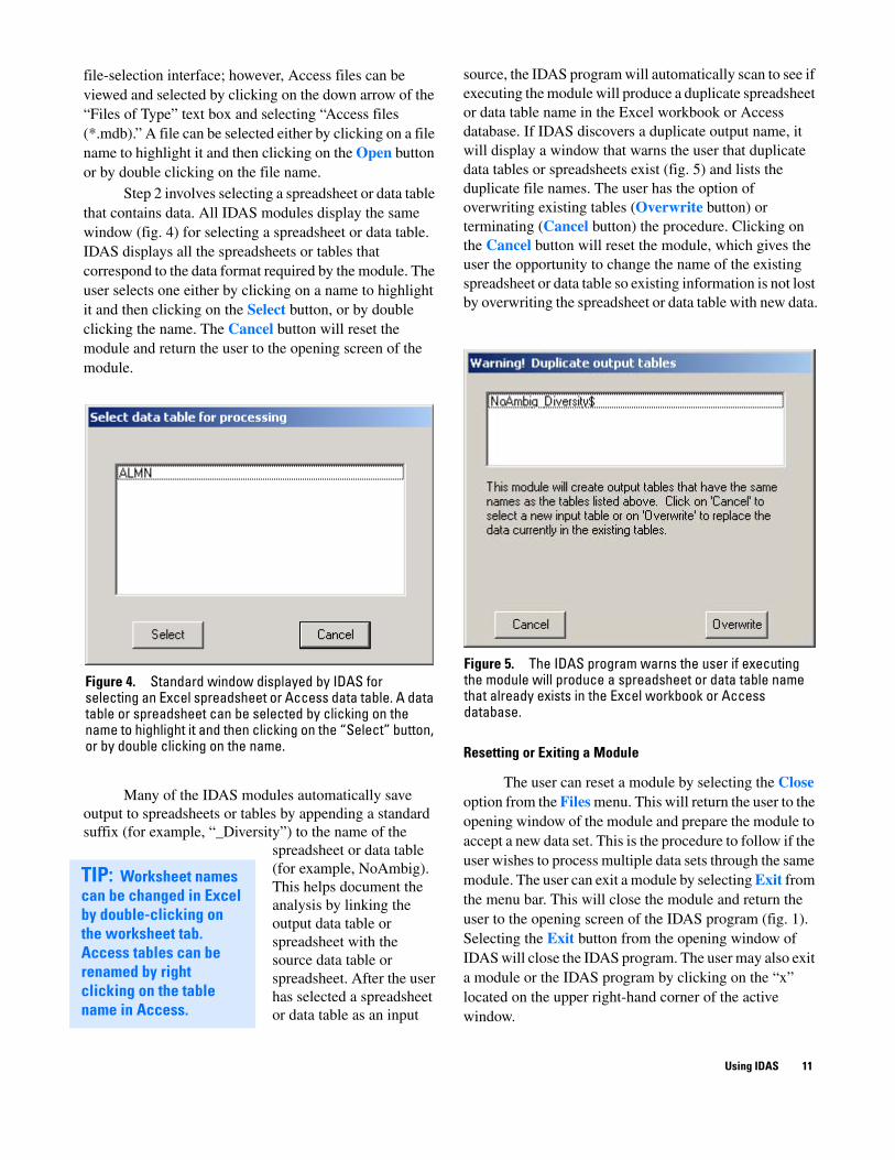
file-selection interface; however, Access files can be viewed and selected by clicking on the down arrow of the “Files of Type” text box and selecting “Access files (*.mdb).” A file can be selected either by clicking on a file name to highlight it and then clicking on the Open button or by double clicking on the file name.

Step 2 involves selecting a spreadsheet or data table that contains data. All IDAS modules display the same window (fig. 4) for selecting a spreadsheet or data table. IDAS displays all the spreadsheets or tables that correspond to the data format required by the module. The user selects one either by clicking on a name to highlight it and then clicking on the Select button, or by double clicking the name. The Cancel button will reset the module and return the user to the opening screen of the module.

Figure 4. Standard window displayed by IDAS for selecting an Excel spreadsheet or Access data table. A data table or spreadsheet can be selected by clicking on the name to highlight it and then clicking on the “Select” button, or by double clicking on the name.

Figure 5. The IDAS program warns the user if executing the module will produce a spreadsheet or data table name that already exists in the Excel workbook or Access database.

Many of the IDAS modules automatically save output to spreadsheets or tables by appending a standard suffix (for example, “_Diversity”) to the name of the

spreadsheet or data table (for example, NoAmbig). This helps document the analysis by linking the output data table or spreadsheet with the source data table or spreadsheet. After the user has selected a spreadsheet or data table as an input

TIP: Worksheet names can be changed in Excel by double-clicking on the worksheet tab. Access tables can be renamed by right clicking on the table name in Access.

source, the IDAS program will automatically scan to see if executing the module will produce a duplicate spreadsheet or data table name in the Excel workbook or Access database. If IDAS discovers a duplicate output name, it will display a window that warns the user that duplicate data tables or spreadsheets exist (fig. 5) and lists the duplicate file names. The user has the option of overwriting existing tables (Overwrite button) or terminating (Cancel button) the procedure. Clicking on the Cancel button will reset the module, which gives the user the opportunity to change the name of the existing spreadsheet or data table so existing information is not lost by overwriting the spreadsheet or data table with new data.

Resetting or Exiting a Module

The user can reset a module by selecting the Close option from the Files menu. This will return the user to the opening window of the module and prepare the module to accept a new data set. This is the procedure to follow if the user wishes to process multiple data sets through the same module. The user can exit a module by selecting Exit from the menu bar. This will close the module and return the user to the opening screen of the IDAS program (fig. 1). Selecting the Exit button from the opening window of IDAS will close the IDAS program. The user may also exit a module or the IDAS program by clicking on the “x” located on the upper right-hand corner of the active window.

Using IDAS 11

EDIT DATA MODULE

The Edit Data module allows the user to subset data, combine and(or) delete data, or summarize the distribution of taxa among sites and samples (fig. 6). This is the only module in the IDAS program that can use data in both Bio-TDB format (appendix table I-1) and processed format (appendix table II-1). The View, Exit, and About menus work the same in this module as in other modules. However, the Files menu in the Edit Data module differs from the files menus in other modules by having a series of submenu items under the Open data files option (fig. 6). These submenus activate processing

options that have different requirements for when and how they open files, spreadsheets, and(or) data tables.

Subset Data

By selecting Subset data, two additional choices (by Sample information and by Taxonomy) can be selected by the user to separate the original data sets into subsets based on sample identifiers (for example, SUID, STAID, and SampleType) or taxonomic groupings (for example, Trichoptera or Ephemeroptera). Clicking on one of these choices will call up the standard file selection (fig. 3) and data table or spreadsheet selection (fig. 4)


Figure 6. The opening screen of the Edit Data module, which differs from other modules in that the “Files” menu contains a series of submenu items under the “Open data files” option. This example shows the selection of the “Subset data by taxonomy” option.

windows. However, since the Edit Data module can process files from both Bio-TDB and processed formats, the user must specify the type of file to be worked with by using the file-type selection window (fig. 7) before the data table or spreadsheet selection window is displayed. Once the user selects a spreadsheet or data table to work on and the IDAS program establishes that the format is correct, then the View menu is activated.

Figure 7. File-type selection window used in the Edit Data module. This example shows that the user has elected to process data that are stored in the original Bio-TDB format.

Figure 8. Selection window used to subse

TIP: Multiple items in the “source” and “destination” windows can be selected by using the shift and control keys in conjunction with the mouse.

Sample Information

The by Sample information option calls up a selection window (fig. 8) that allows the user to subset data based on any combination of SUID, STAID, Reach, CollectionDate, SampleID, sample code (SMCOD), and SampleType (for example, R = RTH, D = DTH, Q = QMH). Once the user has selected an element of sample information to subset, the sample information box is disabled (dimmed) until the user has indicated what action is to be applied to the data. The selected sample information is transferred to the Source file list box. Data to be subset are transferred between the Source file list box and the Destination file list box by double clicking the desired item or by highlighting the desired items (multiple selections are allowed using the shift and control keys in conjunction with the mouse) and clicking on the Transfer button. The Accept button is used to prompt IDAS to act upon the user’s selections.

Once the user selects the Accept button, the appropriate Sample Information check box is checked, provided that the user actually selected items to transfer to

Edit Data Module 13

t data based on sample information.

the destination file. If the user did not select items to send to the destination file, then the Sample information check box will remain unchecked. In this way, the user can quickly see what items of sample information have been selected. The user can click on previously selected Sample information check boxes to review or modify selections. If one or more boxes are checked, the Process button will be activated, which implements the subsetting procedures. Once the Process button has been activated and the user has finished selecting items to subset by, subsetting is implemented by clicking on the Process button. The user will be prompted for the name of a new spreadsheet or data table in which to store the subset of data (fig. 9), or warned that the combination of sample information selected did not correspond to any data in the source file. The name of the new spreadsheet or data table must be 15 characters or less and contain only letters, numbers, and the underscore character. The IDAS program will warn the user if the name entered does not meet these criteria. The new spreadsheet or data table is stored in the original workbook or database.

The IDAS program will display FINISHED in the right-hand status bar panel (fig. 8) when it has finished processing and saving data. The Files/Close menu items can then be used to reset the module and begin processing another data set.

The by Sample information subsetting option is a very important feature of the IDAS program. It allows the analyst to select samples that need to be processed together. For example, the analyst can create data sets that consist only of trends sites, or sites that are part of specific topical studies (for example, land-use gradient studies), or data from specific time periods. This subsetting option also can be used to separate qualitative samples, which should be analyzed separately, from quantitative samples. Breaking down the large data sets exported from Bio-TDB into smaller, more coherent data sets is important for data analysis and program performance because smaller files can be processed faster and more efficiently than larger ones.

Taxonomy

The by taxonomy option calls up a new selection window (fig. 10) that allows the user to select subsets of data based on taxonomy. Taxonomic groups are selected by clicking on the appropriate active check boxes, which are activated only if the taxon exists in the data set. Selected taxa are sent to a new spreadsheet or data table by clicking the Process button. The user will be prompted for a valid spreadsheet or data table name (fig. 9), and the new data will be stored in the original Excel workbook or

Access database. After saving the selected data, the IDAS program updates the selection window by deactivating (dimming) the check boxes that were previously selected. That is, active check boxes correspond only to taxa that exist in the data set and that have not yet been saved to a new spreadsheet or data table. In this way, a data set can be iteratively subset until no taxa remain and only the Quit button remains active. The Quit button or the menu commands Files/Close can be used to reset the subset by taxonomy function and return to the opening screen of the Edit Data module.


Figure 9. Form used to enter a data table or spreadsheet name to store data.

TIP: Tables are automatically appended to the original Excel workbook or Access database following processing.

Figure 10. Selection window used to subset data based on taxonomic information. Taxonomic groups that are not present in the source data file are disabled (dimmed).

Subsetting by Taxonomy can be used to create separate data sets for specific taxonomic groups. These data sets can then be processed through the other modules to calculate metrics or apply different data preparation options to specific taxonomic groups. For example, the analyst may want to process midges (Chironomidae) with a different lowest taxonomic level than other invertebrates. Alternatively, the analyst may want to preserve information on the lifestages of beetles (Coleoptera) but not other invertebrates. Once the subsets of data have been created and processed, they can be recombined by using the Combine/delete option of this module and run through other IDAS modules to calculate metrics, diversities, similarities, or to export data to other analysis packages.

Combine/Delete Data

The Combine/delete data option produces two additional choices (Combine tables/spreadsheets and

Delete tables/spreadsheets) that allow the user to form new data tables or spreadsheets by combining Excel spreadsheets or Access tables of similar types (that is, either Bio-TDB or processed format) or to delete spreadsheets or data tables of all types. By clicking on one of these choices, a file-selection window (fig. 3) appears. If the “Combine tables/spreadsheets” option is selected, the type of file to combine must be selected by using the Select type window (fig. 7). This window will not appear if the “Delete tables/spreadsheets” option is selected, as this option applies to any spreadsheet or data table. Once the user selects a spreadsheet or data table to work on and the IDAS program establishes that format of the spreadsheet or data table is correct, then the View menu item is activated.

Both the combine and delete functions use a source (left) and destination (right) list box to select tables or spreadsheets to combine or delete (fig. 11). The contents of a spreadsheet or data table highlighted in either list box can be viewed by using the View menu item, which will display the first 20 lines of the data table.

Edit Data Module 15

Figure 11. Selection window used to select data tables or spreadsheets to combine. A similar window is used to delete data tables or spreadsheets.

Data tables or spreadsheets can be transferred between the source and destination list boxes by highlighting the file

name(s) and selecting the appropriate Transfer button or by double-clicking the data table or spreadsheet file name. Data are combined or deleted by selecting the Combine or Delete buttons. The IDAS program prompts the user for the name of a new data table or spreadsheet in which to store the

combined data (fig. 9), but it gives no further warning if data tables or spreadsheets are being deleted. Once data tables or spreadsheets have been deleted, they cannot be recovered. Therefore, caution should be exercised when selecting the delete option. When data tables or spreadsheets are combined, the original data tables or spreadsheets are kept intact.

The combine and delete functions use the Files/Close menu combination to reset the module. This returns the user to the opening screen of the Edit Data module and prepares the module for processing another data set.

The combine function can be very useful to recombine data sets that were subset on the basis of taxonomy or sample information. The recombined data set can then be run through the other IDAS modules to calculate community metrics, diversities, similarities, or exported to other software packages. The delete function allows the user to eliminate unwanted data without having to exit the IDAS program. This function is particularly useful for deleting Access tables, because Access does not allow the user to delete multiple tables simultaneously.

Summarize Taxa

The Summarize taxa option calculates statistics on the distribution of taxa among samples and sites. Selecting this option from the Files menu produces a file-selection window (fig. 3) followed by a file-type selection

WARNING: Once data tables or spread-sheets have been deleted in the Edit data module, they cannot be recovered! Exercise caution when using the delete capability.


window (fig. 7) and then a data table or spreadsheet selection window (fig. 4). The file-type selection window is required because the Summarize taxa option applies to files in both Bio-TDB (appendix table I-1) and processed formats (appendix table II-1). The user also has the option of summarizing distributions based on BU_ID or the combination of BU_ID and lifestage using the lifestage summarization window (fig. 12). Once the user selects a spreadsheet or data table to work on and the IDAS program establishes that the format is correct, then the View menu item is activated. The View menu is used to view the first 20 rows of the selected spreadsheet or data table.

Figure 12. The distribution of taxa can be summarized based on BU_ID or the combination of BU_ID and lifestage.

TIP: Use the “Summarize taxa” function of the Edit Data module to investigate how to resolve ambiguous taxa and to set limits for deleting rare taxa.

The IDAS program summarizes the distribution of taxa and saves this information in the source file by using a data table or spreadsheet name that contains the input data table name (for example, ALMN) plus the suffix “_Distrib” (for example, ALMN_Distrib). The Summarize taxa function summarizes the distribution of taxa across a group of samples. The summary contains the

list of taxa (rows) in phylogenetic order with the taxonomic hierarchy plus the following columns of information:

BU_ID: name of the taxon being summarized.

Lifestage: “A” for adult, “P” for pupae, “L” for larvae, or blank.

Ambig: indicates if the taxon is ambiguous (“Yes”) or not (blank).

noChild: number of children that are associated with an ambiguous taxon.

sumChild: sum of the abundances of children associated with an ambiguous taxon.

pSumChild: percentage of total abundance represented by sumChild.

Sites: number of sites where the taxon occurs.pSites: percentage of sites where the taxon occurs.Samples: number of samples in which the taxon occurs.pSamples: percentage of samples in which the taxon

occurs.Abund: the abundance of the taxon summed in all samples.pAbund: percentage of total abundance represented by

Abund.Ave_All: average abundance of taxon in all samples.MAX_All: maximum abundance of taxon in all samples.MIN_All: minimum abundance of taxon in all samples.StDev_All: standard deviation of abundance of taxon in all

samples.Ave_Occur: average abundance of taxon in samples where

it occurs.MAX_Occur: maximum abundance of taxon in samples

where it occurs.MIN_Occur: minimum abundance of taxon in samples

where it occurs.StDev_Occur: standard deviation of abundance of taxon in

samples where it occurs.

Average, maximum, minimum, and standard deviation of abundances are given based on consideration of all (_All) samples (that is, abundance is considered to be zero for samples in which the taxon does not occur) and considering only samples in which the taxon actually occurs (_Occur). Processing data through the Summarize taxa function is an important preliminary step in the analysis of invertebrate data. The statistics generated by this function allow the analyst to get a comprehensive overview of the data, which can be helpful in deciding how to resolve ambiguities, subset data, set limits for deleting rare taxa, or in providing a taxa list for a group of samples.

DATA PREPARATION MODULE

The Data Preparation module prepares data for analysis by the other modules. This module reads abundance data exported from Bio-TDB (combined results format, appendix table I-1) and produces a new file format (processed format, appendix table II-1) that can be read by the other IDAS modules. There are two main objectives in data preparation: (1) resolve taxonomic ambiguities in the data and (2) combine data so that rows of data correspond to taxa richness (where a taxon is represented by a BU_ID or a combination of BU_ID and lifestage). The Data Preparation module provides the following functionalities:

1. Select sample types (QMH, DTH, RTH, and(or) QUAL = QMH+RTH+DTH) to process.

Data Preparation Module 17

2. Calculate densities (no./m2) using the sample area information contained in the file “_Sample_All.xls” exported by Bio-TDB (appendix table I-2).

3. Delete data based on NWQL BG processing notes such as immature or damaged.

4. Delete pupae or non-aquatic adult insects.

5. Combine or retain information on lifestages.

6. Select how to form QUAL samples: QMH+RTH and(or) DTH.

7. Select a lowest taxonomic level (family, tribe, genus) for the data set.

8. Delete rare taxa based on the percentage of total abundance in a sample and(or) the percentage of sites at which the taxon occurs.

9. Resolve ambiguous taxa separately for each sample or for a combination of samples using one of five methods:

A. Delete ambiguous parents and retain children.B. Delete children of ambiguous parents and add

their abundance to the parent.C. Retain abundance of children if it is larger than

the abundance of parents. Otherwise, combine children with parents.

D. Distribute ambiguous parent’s abundance among children in accordance with their relative abundance.

E. None: retain ambiguous taxa.

The Files, View, Exit, Run, and About menus operate the same as in other modules. The Status menu option is used to display a separate window that tracks the progress of the IDAS program as it performs the various processing steps requested by the user. The Options menu allows the user to select the order for displaying the children of an ambiguous parent — alphabetically or by occurrence (that is, descending order based on the number of sites where each taxon is found). Once an appropriate (that is, combined results Bio-TDB format) Excel spreadsheet or Access data table is selected for processing and the data format and contents are checked, the IDAS program displays the various options for data preparation (fig. 13) and activates the Run menu. If the user selects Run without selecting any options, the resulting file will have a different format and fewer rows of data than the original file. This is because the Data Preparation module removes, at a minimum, duplicity in BU_ID’s (or BU_ID + Lifestage) associated with NWQL BG sample- processing notes (table 2).

Processing Options

The Data Preparation module provides a large number of options for processing invertebrate data. These options allow the user to produce data sets that emphasize different characteristics of the data for specific analyses (for example, qualitative lists of taxa associated with a site). Collectively, these options provide a powerful set of tools for manipulating NAWQA Program invertebrate data.

TIP: Data must be processed by the Data Preparation module before they can be processed by the Calculate Community Metrics, Calculate Diversities and Similarities, and Data Export modules.


Figure 13. Main window of the Data Preparation module with the processing options displayed.

IP: Don’t combine ualitative (QMH, QUAL) nd quantitative (RTH, DTH) amples in the same data reparation run. Applying uantitative criteria to ualitative data can have nanticipated effects on

he resulting data. eparate data files should e created for qualitative nd quantitative samples.

DAS is designed to do this n the Data Preparation

odule without having to eopen the source file.

Select Sample Type(s) to Process

The Select sample type(s) to process option allows the user to choose which samples to process: QMH, RTH, DTH, and(or) QUAL samples. QUAL samples are synthetic samples that are intended to provide a comprehensive taxa list for a site, reach, and date. They are formed by combining QMH, RTH, and DTH samples associated with a unique combination of SUID, STAID, Reach, and a range of collection dates (CollectionDate) centered upon the QMH sample-collection date. If the user elects to create QUAL samples, the IDAS program

will prompt the user to specify a date range (within ± 0 to 7 days of the QMH sample-collection date) over which it will search for RTH and DTH samples to combine (fig. 14) with QMH samples. RTH and DTH (Cuffney and others, 1993) samples are paired with QMH samples if they have the same SUID, STAID, Reach, and if their collection dates fall within the range specified by the user.

The date range for QUAL aggregation is an acknowledgment that it is not always possible to collect all samples at a site on the same day. If the IDAS program finds multiple RTH or

TqaspqqutSbaIimr


Figure 14. Form for selecting the range of dates over which to aggregate RTH, DTH, and QMH samples when creating the QUAL sample.

DTH samples that can be matched with the QMH sample, it will display an input screen that allows the user to select which RTH and(or) DTH samples are to be paired (fig. 15) with the QMH sample. Each list box also contains a blank line at the bottom that can be used to remove a selection. Only one RTH and(or) DTH sample can be paired with

20 User’s Manual for the National Water-Quality Assessment Program Inv

Figure 15. Data entry screen for selecting RTH and(or) DTH saformation of a QUAL sample. This screen appears when there awith a QMH sample. The user must select the appropriate RTH asample.

each QMH sample. Selecting the Cancel button terminates sample processing and returns to the opening screen of the Data Preparation module. The Accept selection button associates the QMH sample with the selected RTH and DTH samples. The IDAS program automatically documents which RTH and DTH samples are associated with each QMH sample during the creation of the QUAL samples. This documentation consists of the following columns of information that are stored in a spreadsheet or data table with the suffix “_QQSMCODs” (for example, ALMN_QQSMCODs; appendix table II-2).

SUID: four-character abbreviation for Study Unit.STAID: station number.Reach: sampling reach.CollectionDate: date that the QMH sample was collected.Qsmcod: the SMCOD used to identify the QUAL sample.

This SMCOD is generated by setting the “M” identifier in a QMH SMCOD to “Q” (for example, IQM becomes IQQ).

QsampleID: sampleID for the QUAL sample. This is generated by negating the SampleID assigned to the QMH sample (for example, 7770 becomes – 7770).

QMHsmcod: SMCOD assigned to the QMH sample.QMHsampleID: SampleID assigned to the QMH sample.

ertebrate Data Analysis System (IDAS) Software: Version 3

mples to pair with a QMH sample in the re multiple RTH and(or) DTH samples to pair nd(or) DTH samples to pair with the QMH

TIP: The list boxes associated with “RTH choices” and “DTH choices” include a blank line at the bottom that can be selected to clear the entries in the “RTH SMCOD” or “DTH SMCOD” text boxes.

RTHsmcod: SMCOD assigned to the RTH sample.RTHsampleID: sampleID assigned to the RTH sample.DTHsmcod: SMCOD assigned to the DTH sample.DTHsampleID: sampleID assigned to the DTH sample.

Calculate Densities

The Calculate density option allows the user to convert abundance (number/sample) data associated with quantitative (RTH and DTH) samples to density (no./m2) data. This feature is disabled if the user has chosen to process only qualitative data (QMH and(or) QUAL). If the user chooses to calculate densities, the program

prompts the user to select a spreadsheet or data table that contains information on the area sampled for each RTH or DTH sample. This information is contained in Bio-TDB export files of the form “_Sample_All.xls” (for example, ALMN_10302001_1052_

Sample_ All.xls). If the program cannot find sample area information for a sample, it alerts the user and provides the option of continuing without the sample or quitting the analysis and returning to the opening screen of the Data Preparation module. The user must check to make sure that the “_Sample_All.xls” file contains accurate sample area information; otherwise the densities generated will be in error. If qualitative samples (QMH or QUAL) are present in the data being processed, the densities for these samples will automatically be set to one (1).

Densities should be calculated when the sampling areas associated with the samples in the data set are variable and the analyses include comparing abundances

among samples. If all sampling areas are the same for all samples (for example, composites of five Slack samplers) or the analytical techniques to be used are strictly qualitative, then densities do not need to be calculated.

Data Deletions Based on NWQL BG Processing Notes

The IDAS program allows the user to delete rows of data based on the NWQL BG sample-processing notes (Notes column, appendix table I-1) associated with each row. The IDAS program recognizes six standard sample-processing notes (Moulton and others, 2000) that can be combined and used to delete data (table 5). One of three options can be selected for each type of laboratory sample-processing note (fig. 13): none, all taxa, and ambig taxa. None is the default option, and selecting this option results in no deletions. The All taxa option will delete all lines of data where the sample-processing note appears. The Ambig taxa option will only delete a line of data if the note is present and the taxon is ambiguous within the sample. In table 6 the various options are shown for the sample-processing note “imm.” (immature). The option none does not alter the data; the All taxa option deletes all data with the string “imm.” in the processing notes column; Ambig taxa deletes only data with “imm.” noted in association with an ambiguous taxon (Hydropsychidae). This option does not delete data when “imm.” is associated with a non-ambiguous taxon (Hydropsyche).

Processing notes provide a means for the NWQL BG taxonomist to communicate problems with data quality to the analyst. The analyst can then decide whether to eliminate poor-quality data (for example, damaged specimens) based on these notes. For example, eliminating damaged (dam.) and immature (imm.)

TIP: Sample area information is located in the Sample_All.xls file in Bio-TDB.


Table 5. National Water Quality Laboratory Biological Group (NWQL BG) standardized sample-processing notes (Moulton and others, 2000) that are recognized by the IDAS program [The user can delete rows of data based on any combination of these notes]

Notes Description

imm. Immature: identification to a prescribed level is not supported because the organism(s) is(are) too immature.

dam. Damaged: identification to a prescribed level is not supported because the organism(s) is(are) damaged.

Mount Poor mount: identification to a prescribed level is not supported because slide-mounted organism(s) is(are) poorly oriented on slide.

indet. Indeterminate: identification to a prescribed level is not supported for recently molted organisms, mayfly subimagos, or mature and intact organisms because of undocumented variation or indistinct characters, required case is missing or damaged, or required habitat or ecological information is missing or unavailable.

Gender Gender: identification to targeted level is not supported because of gender.

Artifact Artifact: taxon is not represented by a complete organism (for example, bryozoan fragment or empty mollusk shell).

Table 6. The three options for applying NWQL BG sample-processing notes operate differently if ambiguous taxa are present. In this example, Hydropsychidae is an ambiguous taxon

Original dataBU_ID

Abundances after processing notes using option:

Abundance Notes None All taxa Ambig taxa

Hydropsychidae 10 imm. 10 0 0

Hydropsyche 20 dam., imm. 20 0 20

Ceratopsyche 30 30 30 30

specimens can be an effective method for reducing taxonomic ambiguities in the data. Using the Ambig taxa option of this function will minimize the loss of taxa richness in samples by restricting the elimination of taxa to those instances when the taxa are ambiguous. The decision on whether to delete taxa based on processing notes depends on the amount of information (taxa richness and abundance) that will be lost in relation to the reduction in ambiguous taxa.

Data Deletions Based on Lifestages

The Deletions based on lifestages option allows the user to delete all lines of data with a lifestage listed as “P” for pupa and(or) data that correspond to non-aquatic adult insects. Non-aquatic adult insects are defined as adults in the orders Ephemeroptera, Odonata, Plecoptera, Megaloptera, Neuroptera, Trichoptera, Lepidoptera, Hymenoptera, and Diptera. Adults in the orders Orthoptera, Hemiptera, and Coleoptera will be retained even if the user selects the delete adult lifestages (terrestrial adults only) option. The program default is to retain pupae and drop non-aquatic adult insects. Table 7C is an example of how this function works in relation to deletions based on BG notes and lifestages. Adults of the caddisfly Hydroptila are eliminated, but not adults of the beetle Optioservus.

The methods for collecting invertebrate samples in the NAWQA Program (Cuffney and others, 1993; Moulton and others, 2002) are not designed to collect aquatic insects during the terrestrial stage of their lifecycles. Any such adults that are collected are not of much value in community assessments because their place of origin is unknown. Therefore, it is recommended that terrestrial adults be deleted, which is why this is a default in the IDAS program. Pupae should be retained for analysis because they represent the completion of the aquatic phase of the lifestage and are a part of the invertebrate community at the site.

Options Based on Combining Lifestages

The choices under Options based on combining lifestages allow the user to keep lifestages (A = adult, P = pupa, L = larva) separate or to combine lifestages. If the user elects to keep lifestages separate, then a taxon is identified by the combination of BU_ID and lifestage, and the processed data can have multiple BU_ID’s within a sample (for example, Lara L, Lara A, and Lara P). If the user elects to combine lifestages, there only will be one BU_ID within a sample and information on lifestage will be lost (for example, Lara). It is important for the user to realize that this option will always combine data within a sample based either on BU_ID or BU_ID + lifestage. The resulting data sets usually will have fewer rows than the original data because the data are combined without regard to the NWQL BG sample-processing notes. Combining data on the basis of BU_ID or BU_ID + lifestage requires combining lab notes, which renders this information useless as a means of identifying data-quality problems. Consequently, lab notes are deleted at this point in data preparation.

Options for handling laboratory processing notes and lifestages can have important consequences in the calculation of metrics by later modules that assume each row in a sample corresponds to a unique taxon. The effects of these options on estimates of abundance and richness are illustrated in table 7. By eliminating immature organisms, total abundance is reduced from 248 to 133 and the number of lines of data (richness) from 8 (table 7A) to 6 (table 7B). An example of the effects of deleting non-aquatic adult insects is given in table 7C in which adults of the caddisfly Hydroptila were deleted but adults of the beetle Optioservus, which are aquatic adults, were not. The number of rows (richness) was reduced from 6 to 5 and total abundance changed from 133 to 128. In table 7D the results of combining lifestages are a reduction in the number of lines of data (richness) from 5 to 2 but no change in total abundance. The effects of retaining lifestages can be seen in table 7E in which the number of lines of data (richness) was reduced from 5 to 4, but total abundance remained the same as in table 7C.



Table 7. Examples of how the IDAS program can modify data using sample-processing notes (Notes) and lifestage data. How the data are combined affects the number of rows in the data (richness) and the total abundance in the processed sample

A. Data prior to processing:BU_ID Lifestage Notes Abundance


Hydroptila sp. P 5

Hydroptila sp. A 5

Hydroptila sp. L imm. 50


Hydroptila sp. L dam., imm. 65

Optioservus sp. A 20

Optioservus sp. L 40

Taxa richness 8

Total 248

B. Data after eliminating organisms too immature (imm.) to identify (using option “All taxa”):



Hydroptila sp. P 5

Hydroptila sp. A 5




Taxa richness 6

Total 133

C. Data after eliminating immature (all) and non-aquatic adult insects:BU_ID Lifestage Notes Abundance


Hydroptila sp. P 5




Taxa richness 5

Total 128

D. Data after eliminating immature (all), non-aquatic adult insects, and combining lifestages:


Hydroptila sp. 68

Optioservus sp. 60

Taxa richness 2

Total 128

E. Data after eliminating immature (all), non-aquatic adult insects, and keeping lifestages separate:


Hydroptila sp. L 63

Hydroptila sp. P 5



Taxa richness 4

Total 128

Since these processing options can have a significant effect on richness and abundance, the user must carefully consider how the options selected can affect the processed data.

Options for Forming Qualitative (QUAL) Samples

The choices under Options for forming qualitative (QUAL) samples allow the user to specify the sample types to be used in forming the QUAL sample. The user can elect to combine all sample types (QMH + RTH + DTH) or (RTH + QMH) or (DTH + QMH). Even though the DTH samples are no longer collected in the NAWQA Program (Moulton and others, 2002), some DTH samples may be present in earlier data sets (Cuffney and others, 1993). This option provides the user with a simple means of controlling the types of data that are used in forming QUAL samples. The default option (RTH + QMH) will ensure comparability in the creation of QUAL samples for NAWQA data sets collected at any time.

The IDAS program automatically creates new SampleID’s and SMCOD’s for the QUAL samples based on the QMH samples that form the basis of the QUAL samples. QUAL SampleID’s are set to the negative value of the QMH SampleID (for example, 7909 becomes – 7909). The sample component designator in the QMH SMCOD (“M”) is set to “Q” for the QUAL SMCOD (for example, ALMN0695IQM0063 becomes ALMN0695IQQ0063). In this way, it is easy to associate a QUAL sample with the QMH sample from which it is derived.

Select Lowest Taxonomic Level

The Select lowest taxonomic level option allows the user to select the lowest taxonomic level that occurs in the data set (phylum being the highest and species being the lowest). This option works by substituting the selected

taxonomic level for lower taxonomic levels in the BU_ID column. Table 8 is an example of how this option operates when the lowest taxonomic level is set to species, genus, family, and order. Once the substitutions are made, the program recombines data on the basis of SampleID, revised BU_ID, and lifestage. The taxonomic hierarchy is then updated to reflect the revised BU_ID’s. The IDAS program generates a SortCode for each of the revised BU_ID’s when one is not already available. This new SortCode is the highest value of the SortCodes associated with the original BU_ID’s that were combined into the new BU_ID. These SortCodes permit the sorting of the data into phylogenetic order, but they may not correspond to the SortCodes in the original data set.

When selecting the lowest taxonomic level for processing, it is important to note that there can be a difference between data sets produced with the lowest taxonomic level set to BU_ID and data sets produced with the lowest taxonomic level set to species. It would seem that using either of these levels would result in identical data sets since species is the lowest taxonomic level provided by the NWQL BG. However, the BU_ID provided by the NWQL BG can contain provisional and conditional identifications. Provisional and conditional identifications (Moulton and others, 2000) occur when a specimen represents a potentially undescribed species or possesses sufficient characteristics to permit its assignment to a pair or group of closely allied species or genera. Provisional and conditional identifications are reported in the BU_ID column of the data exported from Bio-TDB but are not listed in the taxonomic hierarchy associated with the BU_ID (table 3), which lists only definitive identifications. Consequently, when species is selected as the lowest taxonomic level, the resulting data set can be different from that based on BU_ID. For example, in table 8 the BU_ID column contains two provisional taxa: the species Hydropsyche betteni/depravata and the genus Bezzia/Palomyia. When species


Table 8. An example of how the “Select lowest taxonomic level” option operates at the species, genus, family, and order levels

Revised BU_ID when lowest taxonomic level is set at:Original BU_ID Species Genus Family Order

Glossomatidae Glossomatidae Glossomatidae Glossomatidae Trichoptera

Agapetus Agapetus Agapetus Glossomatidae Trichoptera

Glossosoma Glossosoma Glossosoma Glossomatidae Trichoptera

Hydropsychidae Hydropsychidae Hydropsychidae Hydropsychidae Trichoptera

Hydropsyche Hydropsyche Hydropsyche Hydropsychidae Trichoptera

H. betteni H. betteni Hydropsyche Hydropsychidae Trichoptera

H. betteni/depravata Hydropsyche Hydropsyche Hydropsychidae Trichoptera

Ceratopsyche Ceratopsyche Ceratopsyche Hydropsychidae Trichoptera

Bezzia/Palpomyia Ceratopogoninae Ceratopogoninae Ceratopogonidae Diptera

are substituted for BU_ID’s, the provisional and conditional identifications are replaced with definitive identifications at the next highest taxonomic levels, genus (Hydropsyche) and subfamily (Ceratopogoninae), respectively. If the analyst wants to include provisional identifications in analyses, BU_ID must be selected as the lowest taxonomic level. If the analyst does not want to include provisional identifications in analyses, then species must be selected as the lowest taxonomic level. The user can select different lowest taxonomic levels for different taxonomic groups by using the subset by taxonomy function of the Edit Data module to create subsets of data that can be processed by the Data Preparation module and recombined using the Combine data function of the Edit Data module.

Delete Rare Taxa

This option allows the user to delete taxa (based either on BU_ID or BU_ID + lifestage) that occur at only a few sites and(or) that constitute only a small proportion of the abundance in a sample. The concept of deleting rare taxa prior to analysis is somewhat controversial. Users should review the work of Goff (1975), Faith and Norris (1989), Marchant (1990), Marchant and others (1997), and Cao and others (1998; 1999; 2001) to obtain some insight into how removing rare taxa can affect multivariate analyses and metric-based bioassessments.

Four options are available for removing rare taxa. The user can cycle through these options by clicking on the numbered button in the Delete rare taxa frame (fig. 13). Options for deleting rare taxa are based on their occurrence at a certain number of sites (integer) or as a certain percentage (0 – 100) of abundance or density. The available options for deleting rare taxa are as follows:

1. Delete taxa that occur at less than or equal to the specified number of sites in the data set. Then delete taxa that constitute less than or equal to a specified percentage of abundance or density in the sample (delete sites, then abundance). This approach evaluates each element separately. That is, the

number of sites where each taxon occurs is calculated and the taxa that occur at or below the criterion are deleted. The IDAS program then calculates the percentage abundance or density for each of the remaining taxa in each sample and deletes those that occur at or below the criterion.

2. Delete taxa that constitute less than or equal to the specified percentage of abundance or density in each sample. Then delete taxa that occur at less than or equal to a specified number of sites in the data set (delete abundance, then sites). As in option 1, this approach evaluates each element separately. That is, the program calculates the percentage of abundance or density contributed by each taxon in each sample and deletes those that occur at or below the specified criterion. The program then calculates the number of sites where each of the remaining taxa occurs and deletes the taxa that occur at or below this criterion.

3. Simultaneously delete taxa that constitute less than or equal to the specified percentage of abundance (or density) AND that occur at less than or equal to the specified number of sites (delete abundance and sites). This option differs from options 1 and 2 in that the number of sites where each taxon occurs and the contribution of each taxon to total abundance/density in each sample are calculated simultaneously. Then these criteria are applied in a simple combined query, that is, a taxon is deleted if the number of sites where it occurs is at or below the criterion level and if the percentage of abundance or density contributed by the taxon in the sample is less than or equal to the criterion. Both criteria must be met before a taxon can be deleted from a sample.

4. Simultaneously delete taxa that constitute less than or equal to the specified percentage of abundance (or density) OR that occur at less than or equal to the specified number of sites (delete abundance or sites). This option is similar to option 3, except that taxa are deleted if they occur at less than or equal to the criteria for number of sites or they contribute less than or equal to the criterion for the percentage of abundance or density. Taxa are deleted from a sample if they meet either of these criterions.

The user must be aware of the nuances of these procedures before applying them to the data. For example, if a taxon is deleted on the basis of the number of sites where it occurs (note: this is the number of sites (STAID) where the taxon is found not the number of samples

WARNING: The deletion options provided in the IDAS program are powerful and can be complicated. Be sure that you have studied the examples provided and understand how each option works before you select an option to apply to your data! Different options can result in deleting widely different groups of taxa.


(SampleID) in which it is found), then the taxon will be deleted across all samples. However, if a taxon is deleted

on the basis of its contribution to the total sample abundance or density, it will be eliminated only from those samples where it fails to meet the criterion rather than from all samples. Consequently, the order in which deletions are applied in options 1 and 2 (sites then abundance or abundance then sites) can have a profound effect on the taxa that

are deleted because the calculations of occurrence and abundance are conducted sequentially. Similarly, the

operators and and or used in options 3 and 4, respectively, can greatly affect the number of taxa that are deleted and the abundance or density that remains in the processed data set. Examples of these effects are shown in table 9, in which taxa richness and density are shown before and after applying the four options for deleting rare taxa. The same criteria (delete taxa that occur at two sites or less; delete taxa that constitute 1 percent or less of sample abundance) were used in each of the four options. As indicated in table 9, the user’s selection of a deletion option can have a profound effect on taxa richness and abundance.

The following series of examples demonstrate how each of the four deletion options process information on occurrence and abundance or density to identify which taxa to delete. Each example is applied to the hypothetical invertebrate density data presented in table 10 and is based on the same deletion criteria (delete taxa occurring at two or fewer sites; delete taxa contributing 5 percent or less of sample abundance).

TIP: Insight into the appropriate values to enter in the “delete rare taxa” criteria boxes can be obtained by using the “summarize taxa” option in the Edit Data module. This will give a good summarization of the distribution of taxa across sites and samples in the data set.


Table 9. Effects of “delete rare taxa” options 1 – 4 on taxa richness and density [All options are based on the same criteria (delete taxa that occur at two sites or less; delete taxa that constitute 1 percent or less of sample abundance)]

Taxa richnessMethod used to delete rare taxa

Site Original Option 1 Option 2 Option 3 Option 4

Site 1 53 11 20 41 10

Site 2 58 14 26 38 10

Site 3 50 14 19 35 13

Site 4 49 17 28 35 13

Site 5 54 9 19 30 8Density

Method used to delete rare taxa

Site Original Option 1 Option 2 Option 3 Option 4

Site 1 6,373 4,726 5,590 5,967 4,534

Site 2 1,138 823 1,000 1,036 712

Site 3 891 666 740 805 646

Site 4 1,620 1,258 1,479 1,479 1,056

Site 5 6,281 5,003 5,890 5,668 4,730

Table 10. Hypothetical density data used to illustrate how the options for deleting rare taxa determine which taxa to delete[Occurrence is the number of sites where the taxon is found]

Taxon Site 1 Site 2 Site 3 Site 4 Site 5 Occurrence

Spp 1 107.2 1

Spp 2 26.4 1

Spp 3 860.8 63.2 60.8 120.8 128.8 5

Spp 4 476.0 19.2 2

Spp 5 218.4 1

Spp 6 26.4 16.0 45.3 3

Spp 7 23.2 1

Spp 8 5.0 51.2 10.2 3

Spp 9 68.0 1

Spp 10 36.8 22.4 54.4 3

Total 1,449.0 176.0 169.6 298.7 347.2 5

Option 1 (delete sites then abundance) requires three steps to identify and eliminate rare taxa (table 11). Step 1 eliminates all taxa that occur at two or fewer sites (Spp 1, 2, 4, 5, 7, and 9; table 11). Step 2 calculates the percentage of density contributed by the remaining taxa. Step 3 eliminates all taxa that contribute less than 5 percent of abundance in the sample (Spp 8 in samples from sites 1 and 4). Applying option 1 to the data in table 10 results in the loss of 20 to 75 percent of taxa richness, but less than 5 percent of sample density.

Option 2 (delete abundance then sites) requires three steps to identify and eliminate rare taxa (table 12).

Step 1 calculates the percentage of density contributed by each taxon at each site. Step 2 eliminates all taxa that contributed less than 5 percent of the density in each sample (Spp 8 in samples from sites 1 and 4). Step 3 eliminates all taxa that occur at two or fewer sites (Spp 1, 2, 4, 5, 7, 8, 9; table 12). Applying option 2 to the data in table 10 results in the loss of 40 to 75 percent of taxa richness and 27 to 63 percent of sample density. The data set produced by option 2 (table 12) is different from that produced by option 1 (table 11) even though the only difference between the two methods is the order in which the criteria for deletion (occurrence and density) are applied.



Table 11. Examples of the steps used to delete rare taxa in option 1 as applied to the data in table 10[Deletion criteria are delete taxa that occur at two sites or less, then delete taxa that contribute 5 percent or less to sample density]

Step 1: Delete taxa that occur at two sites or less (Spp 1, 2, 4, 5, 7, and 9).


Spp 1 0

Spp 2 0

Spp 3 860.8 63.2 60.8 120.8 128.8 5

Spp 4 0

Spp 5 0

Spp 6 26.4 16.0 45.3 3

Spp 7 0

Spp 8 5.0 51.2 10.2 3

Spp 9 0

Spp 10 36.8 22.4 54.4 3

Total 865.8 126.4 150.4 230.7 128.8

Step 2: Calculate the percentage of total abundance contributed by each taxon after eliminating taxa based on whether they occur at more than two sites.


Spp 1 0

Spp 2 0

Spp 3 99.4 50.0 40.4 52.4 100.0 5

Spp 4 0

Spp 5 0

Spp 6 20.9 10.6 19.6 3

Spp 7 0

Spp 8 0.6 34.0 4.4 3

Spp 9 0

Spp 10 29.1 14.9 23.6 3

Total 100.0 100.0 100.0 100.0 100.0

Step 3: Delete taxa that constitute 5 percent or less of sample abundance (Spp 8 at sites 1 and 4). Total is the percentage of original density that remains.Taxon Site 1 Site 2 Site 3 Site 4 Site 5 Occurrence

Spp 1 0

Spp 2 0

Spp 3 99.4 50.0 40.4 52.4 100.0 5

Spp 4 0

Spp 5 0

Spp 6 20.9 10.6 19.6 3

Spp 7 0

Spp 8 34.0 1

Spp 9 0

Spp 10 29.1 14.9 23.6 3

Total 99.4 100.0 100.0 95.6 100.0


Table 12. Examples of the steps used to delete rare taxa in option 2 as applied to the data in table 10 [Deletion criteria are delete taxa that contribute 5 percent or less to sample density, then delete taxa that occur at two sites or less]

Step 1: Calculate the percentage of total abundance contributed by each taxon.Taxon Site 1 Site 2 Site 3 Site 4 Site 5 Occurrence

Spp 1 7.4 1

Spp 2 15.0 1

Spp 3 59.4 35.9 35.8 40.4 37.1 5

Spp 4 32.9 11.3 2

Spp 5 62.9 1

Spp 6 15.0 9.4 15.2 3

Spp 7 13.2 1

Spp 8 0.3 30.2 3.4 3

Spp 9 22.8 1

Spp 10 20.9 13.2 18.2 3

Total 100.0 100.0 100.0 100.0 100.0

Step 2: Delete taxa that constitute 5 percent or less of sample abundance (Spp 8 at sites 1 and 4).Taxon Site 1 Site 2 Site 3 Site 4 Site 5 Occurrence

Spp 1 7.4 1

Spp 2 15.0 1

Spp 3 59.4 35.9 35.8 40.4 37.1 5

Spp 4 32.9 11.3 2

Spp 5 62.9 1

Spp 6 15.0 9.4 15.2 3

Spp 7 13.2 1

Spp 8 30.2 1

Spp 9 22.8 1

Spp 10 20.9 13.2 18.2 3

Total 99.7 100.0 100.0 96.6 100.0

Step 3: Delete taxa that occur at two sites or less (Spp 1, 2, 4, 5, 7, 8, and 9).Taxon Site 1 Site 2 Site 3 Site 4 Site 5 Occurrence

Spp 1 0

Spp 2 0

Spp 3 59.4 35.9 35.8 40.4 37.1 5

Spp 4 0

Spp 5 0

Spp 6 15.0 9.4 15.2 3

Spp 7 0

Spp 8 0

Spp 9 0

Spp 10 20.9 13.2 18.2 3

Total 59.4 71.8 58.5 73.8 37.1

Option 3 (delete abundance and sites) requires only two steps to identify and eliminate rare taxa (table 13). The first step calculates the percentage of density contributed by each taxon in the sample and the number of sites where the taxa occur (occurrence). The second step eliminates taxa that occur at fewer than two sites and contribute 5 percent or less to sample density. The results from applying option 3 to the data in table 10 are very different from those obtained by using options 1 (table 11) or 2 (table 12). No taxa are eliminated because no taxa meet both criteria. Spp 1, 2, 4, 5, 7, and 9 (table 13) have occurrences that are below the occurrence criterion, but their contribution to sample density is above the criterion so they are not deleted. Similarly, Spp 8 at sites 1 and 4 falls below the criterion for contribution to sample density, but Spp 8 occurs at more than two sites so it is not deleted. In this example, applying option 3 to the

data in table 10 did not change it. Although this would not be the case for other data sets and(or) using other criteria.

Option 4 (delete abundance or sites) is similar to option 3 in that it requires only two steps to identify and eliminate rare taxa (table 14). The first step calculates the percentage of density contributed by each taxon in the sample and the number of sites where the taxa occur (occurrence). The second step eliminates taxa that occur at fewer than two sites or contribute 5 percent or less to sample density. The difference between option 4 and option 3 is the substitution of the “or” operator for the “and” operator used in option 3. In option 3, a taxon must meet both criteria before it can be deleted, whereas in option 4 a taxon must meet only one of the criteria before it can be deleted. Consequently, more taxa are deleted in option 4 than in option 3. The results of using option 4 also differ substantially from the results obtained by using


Table 13. Examples of the steps used to delete rare taxa in option 3 as applied to the data in table 10 [Deletion criteria are delete taxa that occur at two or fewer sites and delete taxa that contribute 5 percent or less to sample density]

Step 1: Calculate the number of sites where each taxon occurs (occurrence) and the percentage of sample abundance contributed by each taxon.Taxon Site 1 Site 2 Site 3 Site 4 Site 5 Occurrence

Spp 1 7.4 1

Spp 2 15.0 1

Spp 3 59.4 35.9 35.8 40.4 37.1 5

Spp 4 32.9 11.3 2

Spp 5 62.9 1

Spp 6 15.0 9.4 15.2 3

Spp 7 13.2 1

Spp 8 0.3 30.2 3.4 3

Spp 9 22.8 1

Spp 10 20.9 13.2 18.2 3

Total 100.0 100.0 100.0 100.0 100.0 5

Step 2: Delete taxa that occur at two sites or less and that contribute 5 percent or less to abundance in the sample. (No taxa are deleted because no taxa meet both of these criteria.)Taxon Site 1 Site 2 Site 3 Site 4 Site 5 Occurrence

Spp 1 7.4 1

Spp 2 15.0 1

Spp 3 59.4 35.9 35.8 40.4 37.1 5

Spp 4 32.9 11.3 2

Spp 5 62.9 1

Spp 6 15.0 9.4 15.2 3

Spp 7 13.2 1

Spp 8 0.3 30.2 3.4 3

Spp 9 22.8 1

Spp 10 20.9 13.2 18.2 3

Total 100.0 100.0 100.0 100.0 100.0

Table 14. Examples of the steps used to delete rare taxa in option 4 as applied to the data in table 10 [Deletion criteria are delete taxa that occur at two or fewer sites or that contribute 5 percent or less to sample density]

Step 1: Calculate the number of sites where each taxon occurs (occurrence) and the percentage of sample abundance contributed by each taxon.Taxon Site 1 Site 2 Site 3 Site 4 Site 5 Occurrence

Spp 1 7.4 1

Spp 2 15.0 1

Spp 3 59.4 35.9 35.8 40.4 37.1 5

Spp 4 32.9 11.3 2

Spp 5 62.9 1

Spp 6 15.0 9.4 15.2 3

Spp 7 13.2 1

Spp 8 0.3 30.2 3.4 3

Spp 9 22.8 1

Spp 10 20.9 13.2 18.2 3

Total 100.0 100.0 100.0 100.0 100.0 5

Step 2: Delete taxa that occur at two sites or less or that contribute 5 percent or less to abundance in the sample. (Spp 1, 2, 4, 5, 7, 8, and 9 are deleted.)Taxon Site 1 Site 2 Site 3 Site 4 Site5 Occurrence

Spp 1 0

Spp 2 0

Spp 3 59.4 35.9 35.8 40.4 37.1 5

Spp 4 0

Spp 5 0

Spp 6 15.0 9.4 15.2 3

Spp 7 0

Spp 8 0

Spp 9 0

Spp 10 20.9 13.2 18.2 3

Total 59.4 71.8 58.5 73.8 37.1

option 1 (table 11) but are identical to the results obtained by using option 2 (table 12). The comparability of results obtained by using options 2 and 4 is serendipitous. Comparisons of these two options using larger data sets and other criteria show that these options give different results (table 9).

Deleting taxa on the basis of their contribution to sample abundance or density does not have any meaning for qualitative samples in which all abundances are equal — that is, all abundances are one (1). Therefore, if the user is processing only qualitative samples (QMH and(or) QUAL), the option to eliminate taxa on the basis of their contribution to sample abundance or density will be inactive (dimmed). This option is active if the user is conducting an analysis that involves quantitative samples (RTH or DTH) or a combination of quantitative and qualitative samples. It is highly recommended that the

Data Preparation module not be used to process mixed qualitative and quantitative data sets. Each data type should be prepared separately and then, if desired, the user can recombine qualitative and quantitative data into a single spreadsheet or data table by using the Combine tables/spreadsheets option of the Edit Data module.

Options for Resolving Ambiguities

This option provides a variety of methods for resolving taxonomic ambiguities. Ambiguities can be

TIP: Analyze quantitative (RTH and DTH) samples separately from qualitative samples (QMH and QUAL). Use the Edit Data module to create separate qualitative and quantitative data sets.


resolved on a sample-by-sample basis (Keeping samples separate) or on a combined-sample basis (Combining all samples). The sample-by-sample method identifies and resolves ambiguities separately for each sample and commonly is used when communities are expected to differ widely based on natural environmental factors (for example, data collected across a large geographic area). The combined-sample method combines all the data into one sample, finds the ambiguous taxa in the combined sample, and then resolves ambiguities in each sample based on the ambiguous taxa identified in the combined sample. This method commonly is used in situations where there is an expectation that the communities would be similar among sites in the absence of anthropogenic effects (that is, studies conducted in areas with relatively uniform environmental settings). When ambiguous taxa are identified on a sample-by-sample basis (Keeping samples separate), there can be substantial differences in the ambiguous taxa among the samples. For example, Baetis sp. L is an ambiguous parent in samples 7896 and 7973 (table 15) because several species of Baetis are present in these samples. However, sample 7650 does not contain any species of Baetis so Baetis sp. L is not an ambiguous taxon in that sample. Similar differences can be seen for Acentrella sp. L, Plauditus sp. L, Pseudocloeon sp. L, and Zygoptera L. In contrast, resolving ambiguities for a combined data set results in a consistent set of ambiguous taxa (Combined samples column, table 15) that are

resolved uniformly across all samples. However, this approach can lead to instances where a sample contains an ambiguous parent, but no children of that parent (for example, Pseudocloeon sp. L, Baetis sp. L, and Zygoptera in sample 7650) are present in the sample. The

IDAS program provides the user with several methods for handling these situations, which are addressed later in the section Associating ambiguous children with ambiguous parents.

The combined method is most appropriately used in situations where the occurrences of taxa are expected to be fairly uniform among sites in the absence of anthropogenic effects. An example of such a data set would be the urban land-use gradient NAWQA studies where sites are chosen within a limited geographical area in which environmental settings are as similar as possible. In these situations, there is an expectation that the same taxa will be found at all sites in the absence of human effects. This makes it possible to extrapolate the identity of missing children based on the composition of other samples in the data set. In contrast, the sample-by-sample method is most appropriately used when analyzing data across large geographic areas (for example, aggregation of data from multiple Study Units) or when the invertebrate fauna are expected to differ

substantially among sites based on natural factors. In these cases, there is no expectation that a taxon that occurs at one site will occur at another. Therefore, it is not appropriate to extrapolate the occurrence of a missing

Ambiguous taxon: A taxon in a data set in which data are reported at one or more lower or higher taxonomic levels in the taxonomic hierarchy. For example, in a sample that contains data for Hydropsychidae, Hydropsyche, and Hydropsyche sparna, all three taxa are considered ambiguous.

Ambiguous parent: A taxon in a group of ambiguous taxa that occurs at a higher taxonomic level than the other taxa in the group. For example, in a sample that contains data for Hydropsychidae, Hydropsyche, and Hydropsyche sparna, both Hydropsychidae and Hydropsyche are ambiguous parents of Hydropsyche sparna, and Hydropsychidae is an ambiguous parent of Hydropsyche.

Ambiguous child: A taxon that occurs at a lower taxonomic level in a group of ambiguous taxa. For example, in a sample that contains data for Hydropsychidae, Hydropsyche, and Hydropsyche sparna, Hydropsyche and Hydropsyche sparna are ambiguous children of the ambiguous parent Hydropsychidae, and Hydropsyche sparna is the ambiguous child of the ambiguous parents Hydropsyche and Hydropsychidae.


Table 15. Hypothetical invertebrate data used to illustrate eight methods for resolving ambiguous taxa [These data include lifestage information (A = adult, P = pupa, L = larvae) and the identity of ambiguous taxa (Ambig = Yes) for each sample (Separate option) and for all sites combined (Combined option). “Occur” is the number of samples where each taxon occurs, and “Abund” is the abundance of the taxon]

Combined samplesSample

Taxon and lifestage7650 7896 7729 7973

Occur Abund Ambig Abund Ambig Abund Ambig Abund Ambig Abund Ambig

Ephemeroptera A 1 2 2

Ephemeroptera L 1 100 Yes 100 Yes

Baetidae L 2 12 Yes 8 Yes 4 Yes

Acentrella sp. L 3 45 Yes 5 Yes 10 Yes 30

Acentrella parvula L 3 71 26 11 34

Acentrella turbida L 2 12 9 3

Baetis sp. L 3 179 Yes 35 100 Yes 44 Yes

Baetis flavistriga L 2 60 6 54

Baetis intercalaris L 2 99 78 21

Baetis pluto L 3 58 12 23 23

Baetis tricaudatus L 2 13 2 11

Plauditus sp. L 2 61 Yes 5 Yes 56

Plauditus cestus L 2 87 34 53

Pseudocloeon sp. L 2 46 Yes 45 1 Yes

Pseudocloeon propinquum L 2 117 5 112

Zygoptera L 2 110 Yes 10 100 Yes

Argia sp. L 1 8 8

Hydropsychidae L 1 50 50

Diplectrona sp. P 2 33 10 23

Total richness 11 10 11 6

Total abundance 322 312 246 283

child at one site based on its occurrence at other sites. Instead, such extrapolations should be limited to the occurrences of children in each sample. The method used to resolve ambiguities can have a profound effect on the abundance and taxa richness in a sample (fig. 16), and these effects must be considered when using the processed data to calculate community metrics or in statistical analyses.

Methods for resolving taxonomic ambiguities are assigned a three-character abbreviation to facilitate referencing each method. These abbreviations begin with the letter ‘R’ (resolve ambiguities), followed by an ‘S’ (sample-by-sample) or a ‘C’ (combined samples), and ending with the number of the method being used (methods 1 – 5, figure 13). Therefore, RC4 represents the resolution (R) method that identifies ambiguities based on combined samples (C) and distributes ambiguous parent abundance among children in accordance with the relative abundance of each child (method 4).

Sample-by-Sample Basis

The sample-by-sample method of resolving ambiguities (Keeping samples separate) processes each sample separately without considering ambiguities that might exist among samples. That is, it does not deal with situations where a taxon in one sample might be an ambiguous parent or child of taxa in another sample (contrast this approach with the combined method). The sample-by-sample method is most appropriately used when there is no a priori expectation that the sites in the data set will have similar communities in the absence of anthropogenic effects. This method is used for analyses across large geographic areas or across areas with complex environmental settings. The five options that are available under the sample-by-sample method have varying effects on how much taxa richness and abundance are preserved (table 16). The choice of option will be based on how comfortable the analyst is with losing richness and(or) abundance in the process of making data sets as comparable as possible.


Table 16. Taxa richness and abundance obtained by using different methods for resolving taxonomic ambiguities [Each method was applied to the four samples listed in table 15. The upper taxa levels in methods RS2 and RC2 were set to phylum]

Taxa richness Abundance

Method 7650 7896 7729 7973 7650 7896 7729 7973

RS5 11 10 11 6 322 312 246 283

RS1 8 7 8 5 212 104 231 239

RS2 7 2 2 1 322 312 246 283

RS3 8 5 8 5 212 304 231 239

RS4 5 7 8 5 322 312 246 283

RC1 9 7 8 5 212 104 231 239

RC2 4 2 2 1 212 212 246 283

RC3 6 6 8 4 138 154 239 213

RC4 9 7 8 5 322 312 246 283

Figure 16. The method selected to resolve ambiguous taxa can have a profound effect on taxa richness and abundance. In this example both taxa richness and total abundance are strongly affected by the choice of processing option (1 – 4) and whether ambiguities are resolved for each sample separately (S) or for all samples combined (C). Results are expressed as a percentage of richness or abundance derived without resolving ambiguities (option RS5) and combining lifestages. Means and 95% confidence intervals are shown based on 90 RTH samples collected as part of the NAWQA Program urban gradient pilot studies.

Option 1 (RS1): Delete ambiguous parents and retain children.

Processing method RS1 identifies the parents that are ambiguous (that is, exist as BU_ID’s and as the parent of another entry in the BU_ID column) in each sample and then deletes them. The children of the ambiguous parent are not modified. The results of this method are

fewer taxa (lower richness) and lower total abundance in a sample that has one or more ambiguous parent. It is most appropriately used in the analysis of qualitative samples when the user is interested in comparing taxa richness among sites and does not consider abundances. It is less useful in situations when abundance is important


because the application of this method can lead to a substantial loss of abundance.

To show how the RS1 option works, it was applied to the data in table 15, which includes lifestage information (table 17). Ephemeroptera L and Baetidae L were dropped from all samples because children exist in the samples where these taxa occur. Ephemeroptera A was not dropped because all of the children associated with Ephemeroptera are larvae (L) rather than adults (A). Consequently, Ephemeroptera A is not an ambiguous taxon, but Ephemeroptera L is an ambiguous taxon. If the data set had been processed with the option to combine lifestages, then Ephemeroptera would not appear in the processed data. Acentrella sp. L, Baetis sp. L, Plauditus sp. L, Pseudocloeon sp. L, and Zygoptera L were dropped in the samples where children exist, but they were retained in the processed data set because they occur without children (that is, they are not ambiguous taxa) in several of the samples. The abundance and taxa richness of the processed samples (table 17) are substantially reduced from those observed in the original data (table 15). Taxonomic ambiguities were removed from each sample but not from the data set. To fully understand how this processing option works, contrast table 17 with the results obtained using the equivalent resolution

method under the “combined” option (method RC1, table 24).

Option 2 (RS2): Delete children of ambiguous parents and add their abundances to the abundance of the ambiguous parent.

Processing option RS2 identifies in each sample the ambiguous parents, the children associated with each ambiguous parent, and the sum of the abundances of the children associated with each ambiguous parent. The IDAS program then adds the children’s abundances to the appropriate ambiguous parent and deletes the associated children. The program does this iteratively, starting at species and progressing up to phylum. This method will result in fewer taxonomic entities (richness) but total abundance will remain unchanged (table 18). This option is appropriate for analysis when the user wishes to preserve abundance at the expense of taxa richness. This is an extremely conservative approach that can result in summarizing the data into a relatively small number of fairly high taxonomic levels. This option should be used with great caution because it eliminates much of the information content of the data set.

The presence of just a few taxa whose BU_ID identifier is at the order or class level can cause method


Table 17. Results obtained by using processing method RS1 (deleting ambiguous parents and retaining children separately for each sample) to resolve ambiguous taxa in table 15 [Occurrence is the number of sites where a taxon occurs (1 sample per site). Taxa are listed by name and lifestage (A = adult, P = pupa, L = larvae)]

Sample

Taxon and lifestage Occurrence 7650 7896 7729 7973

Ephemeroptera A 1 2

Acentrella sp. L 1 30

Acentrella parvula L 3 26 11 34

Acentrella turbida L 2 9 3

Baetis sp. L 1 35

Baetis flavistriga L 2 6 54

Baetis intercalaris L 2 78 21

Baetis pluto L 3 12 23 23

Baetis tricaudatus L 2 2 11

Plauditus sp. L 1 56

Plauditus cestus L 2 34 53

Pseudocloeon sp. L 1 45

Pseudocloeon propinquum L 2 5 112

Zygoptera L 1 10

Argia sp. L 1 8

Hydropsychidae L 1 50

Diplectrona sp. P 2 10 23

Total richness 8 7 8 5


Table 18. Results obtained by using processing method RS2 (deleting children of ambiguous parents and adding their abundances to that of the parents) to resolve ambiguous taxa in table 15 [The upper taxa limit was set to phylum, which conserves the abundance in each sample while reducing the taxa richness. Occurrence is the number of sites where a taxon occurs (1 sample per site). Taxa are listed by name and lifestage (A = adult, P = pupa, L = larvae)]

Sample


Ephemeroptera A 1 2

Ephemeroptera L 1 250

Baetidae L 2 204 223


Baetis sp. L 1 88

Plauditus cestus L 1 53

Pseudocloeon propinquum L 1 112

Zygoptera L 2 10 108



Taxa richness 5 2 2 4


RS2 to aggregate data into a few high taxonomic levels that are not very useful for analysis. This problem arises when a data set contains organisms that have been identified at taxonomic levels that are much higher than the taxonomic levels specified in the sample-processing protocol (Moulton and others, 2000). Typically, this occurs when the NWQL BG identifies fragments of invertebrates in an effort to provide as much information about the contents of a sample as possible. The IDAS program addresses this problem by forcing the user to select an upper taxonomic limit (note: the default for the upper taxa limit is family) for the aggregation of data (fig. 17). Data associated with ambiguous parents above this upper taxonomic limit are deleted before ambiguities are resolved. This prevents method RS2 from aggregating

36 User’s Manual for the National Water-Quality Assessment Program Inv

Figure 17. Pop-up window that prompts the user to select an upper taxonomic limit for the aggregation of data when using ambiguous taxa resolution method 2 (RS2, RC2).

ambiguous taxa into a few, very high taxonomic levels. Non-ambiguous taxa that occur above the upper taxonomic limit are not affected. When the user selects Run from the Data Preparation menu, the IDAS program checks whether the upper taxonomic limit (fig. 17) chosen by the user is higher than the lowest taxonomic level (fig. 13). If not, an error message (fig. 18) is generated, and the user is prompted to change either the upper taxonomic limit for aggregation or the lowest taxonomic level.

The upper taxa limit selected for aggregation can have a profound effect on the results, both in richness and abundance, obtained by using this method. This is illustrated in table 19, which shows how selecting various upper taxa limits affect the processed data set. For example, setting the upper taxa limit to genus results in the elimination of ambiguous parents that are above this taxonomic level (that is, Arthropoda L, Insecta L, Ephemeroptera L, Leptophlebiidae L, and Hydropsychidae L), but ambiguous parents that are at this taxonomic limit (Acentrella sp. and Plauditus sp.) are retained. Non-ambiguous taxa that are above the upper taxa limit (Turbellaria) are not eliminated. As the upper taxa limit increases, the ambiguous taxa are aggregated into a smaller number of taxonomic entities and taxa richness decreases. In contrast, the proportion of original abundance that remains in the processed data set increases as the upper taxa limit increases because fewer taxa are being eliminated and more taxa are being aggregated. When the upper taxa limit is equivalent to the highest taxonomic level associated with an ambiguous parent

ertebrate Data Analysis System (IDAS) Software: Version 3

Figure 18. Error message generated when the upper taxa limit for resolving ambiguities is lower than the level chosen as the lowest taxonomic level. The information in parentheses indicates where the conflict lies.

Table 19. Results obtained by specifying different upper taxa limits in the RS2 processing method[Ambiguous parents are identified (Ambig = Yes) in the original data]

Taxonomiclevel

Original data Upper taxa limit

Taxon and lifestage Value Ambig Genus Family Order Class Phylum

Turbellaria Class 14 14 14 14 14 14

Arthropoda L Phylum 10 Yes 389

Insecta L Class 25 Yes 379

Ephemeroptera A Order 2 2 2 2 2 2

Ephemeroptera L Order 100 Yes 318

Leptophlebiidae L Family 65 Yes 68

Habrophlebia vibrans L Species 3 3

Acentrella sp. L Genus 5 Yes 31 31

Acentrella parvula L Genus 26

Baetis sp. L Genus 35 35 35

Plauditus sp. L Genus 5 Yes 39 39

Plauditus cestus L Species 34

Pseudocloeon sp. L Genus 45 45 45

Zygoptera L SubOrder 10 1 1 1

Hydropsychidae L Family 23 Yes 26 26

Diplectrona modesta L Species 2 2

Ceratopsyche alhedra L Species 1 1

Taxa richness 17 10 9 5 3 3

Total abundance 405 173 261 361 395 405

(phylum in table 19), then abundance is conserved (that is, the abundance in the processed data is the same as in the original data set). Users are advised to compare the results obtained by using method RS2 with the original data so that they fully understand how this method has altered their data set.

Option 3 (RS3): If the abundance of an ambiguous parent is greater than the sum of the abundances of the children, add the children’s abundances to that of the parent and delete the children; otherwise, retain the children and delete the parent.

Method RS3 works by identifying ambiguous parents and the children associated with them and then comparing the abundance of the ambiguous parents to the sum of the abundances of their children. If the abundance of the ambiguous parent is greater than the sum of the children’s abundances, the children’s abundances are added to the parent abundance and the children are deleted. Otherwise, the parent is deleted and the children are retained. Ambiguities are resolved iteratively, starting with genus and processing up to phylum. The IDAS program keeps track of abundances that are deleted at each taxonomic level and can add these abundances to the


parent in later iterations. This would be necessary if a comparison between an ambiguous parent and its children indicates that the children need to be combined with the parent and one or more parents have been deleted in a previous iteration. Adding the abundances of deleted parents under these circumstances prevents the loss of abundance information. This method results in both reduced sample richness and abundance.

Method RS3 offers a compromise between methods RS1, which eliminates ambiguous parents, and RS2, which eliminates the children of ambiguous parents. This option is used when the analyst wants to tie the preservation of taxa richness to the abundance of the ambiguous taxa and is unwilling to accept the assumptions that are associated with method RS4. Method RS4, which distributes the abundance of ambiguous parents among the children in accordance with the relative abundance of the children, assumes that the ambiguous parents are composed solely of the ambiguous children that occur in the sample (that is, they cannot constitute an unidentified taxon) and occur in proportion to the relative abundance of the ambiguous children. If the user is uncomfortable with these assumptions, method RS3 should be used.

Taxonomic ambiguities are resolved iteratively in method RS3, starting with species and working up to family in the example presented in table 20. The lowest taxonomic level (BU_ID column) is genus, so the first iteration resolves ambiguities between tribe and genus.

Both (Chironomini and Tanytarsini) tribes are ambiguous; that is, each has three genera associated with it. The combined abundance of the children of Chironomini (Chernoushii [10], Chironomus [20], and Cladopelma [5]) is less than the abundance of Chironomini (100) so the abundances of the children are combined with the parent (10 + 20 + 5 + 100 = 135) and the child abundances are set to zero. The opposite is true for the Tanytarsini; the sum of the abundances of the children (65) is greater than the abundance of the ambiguous parent (5). Therefore, the parent’s abundance is set to zero and the children’s abundances are retained. The abundance of the Tanytarsini is transferred to a “carry over” variable so that this abundance is not lost if the children are combined with a parent at a higher taxonomic level in a later iteration. These results are summarized in the “Iteration 1” column of table 20.

The second iteration resolves ambiguities between the first iteration (tribe) and the next taxonomic level (subfamily). Two ambiguous subfamilies are present in this data set — Chironominae and Diamesinae. The abundance of Chironominae (225) is greater than the abundance of the children (Chironomini + Cladotanytarsus + Microspectra + Neozaurelia = 200) so the children’s abundances are added to the parents (225 + 200 = 425). However, the carry over of Tanytarsini (5) from the previous iteration causes the abundance of Chironominae to become 425 + 5 = 430, and the carry over is set to zero. In the case of Diamesinae, the abundance of


Table 20. An example of how processing method RS3 resolves ambiguous taxa over three iterations from genus to family

Taxonomic level Original abundance

Iteration 1:Tribe

Iteration 2:Subfamily

Iteration 3:FamilyFamily Subfamily Tribe Genus (BU_ID)

Chironomidae 100 100 100 0

Chironominae 225 225 430 430

Chironomini 100 135 0 0

Chernoushii 10 0 0 0

Chironomus 20 0 0 0

Cladopelma 5 0 0 0

Tanytarsini 5 0 0 0

Cladotanytarsus 15 15 0 0

Microspectra 20 20 0 0

Neozaurelia 30 30 0 0

Diamesinae 10 10 0 0

Diamesa 15 15 15 15

Pagastia 35 35 35 35

Potthastia 50 50 50 50

Total resolved 640 635 630 530

Carry over 0 5 10 110

Total processed 640 640 640 640

the children (100) is greater than the ambiguous parent’s abundance so the abundance of Diamesinae is set to zero and the abundance of Diamesinae (10) is carried over to the next iteration.

Iteration 3 resolves ambiguities between the subfamily and family levels. In this example the abundance of Chironomidae (100) is less than the sum of the abundance of children (530) so the abundance of Chironomidae is set to zero and the carry-over value becomes 110 (100 Chironomidae + 10 Diamesinae). Resolving ambiguities by using option 3 reduces both the number of taxa and the total abundance in the sample. Results of applying method RS3 to the 4 hypothetical samples presented in table 15 are shown in table 21. These results clearly show that method RS3 is a compromise between methods RS1 and RS2. Method RS3 preserves more of the original taxa richness than does method RS2 (table 19), but less than method RS1 (table 17). In contrast, method RS3 preserves more of sample abundance than does method RS1, but less than method RS2. As with all methods for resolving ambiguities, the user is advised to compare the results with the original data so that the user fully understands how this method has modified the original data before calculating community metrics or exporting data for analysis.

Option 4 (RS4): Distribute ambiguous parent abundance among children in accordance with the relative abundance of each child.

Method RS4 operates by identifying ambiguous parents, the children associated with each ambiguous parent, and the sum of the abundances of the children associated with each ambiguous parent. It then distributes the abundances of the ambiguous parents among the children in accordance with the relative abundance of each child (Ci / Σ Ci, where Ci is the abundance of the ith child). The ambiguous parent is then deleted. Ambiguities are resolved iteratively, starting with genus and working up to phylum. This method resolves ambiguous taxa iteratively, as shown in table 22 for sample 7896 in table 15. The first iteration distributes the abundance of Baetis sp. L among the three species of Baetis (flavistriga, pluto, and tricaudatus) in accordance with the relative abundance of each child. For example, the relative abundance of Baetis flavistriga L is 0.3 (6 / [6 + 12 + 2] ) so 30 percent of the abundance of Baetis sp. L (100 × 0.3 = 30) is added to the abundance of Baetis flavistriga (30 + 6 = 36). The updated abundances are then used as the input for iteration 2, which distributes the abundance associated with the ambiguous family Baetidae (8) among the 6 ambiguous children. As before, this abundance is distributed in accordance with the relative abundance of


Table 21. Results obtained by using processing method RS3 to resolve ambiguous taxa in table 15 [Occurrence is the number of sites where a taxon occurs (1 sample per site). Taxa are listed by name and lifestage (A = adult, P = pupa, L = larvae)]

Sample


Ephemeroptera A 1 2




Baetis sp. L 2 35 120

Baetis flavistriga L 1 54


Baetis pluto L 2 23 23

Baetis tricaudatus L 1 11



Pseudocloeon sp. L 1 45








Table 22. Examples of how processing method RS4 distributes the abundances of ambiguous parents among ambiguous children for sample 7896 in table 15

Iteration 1: Distribute abundance of Baetis sp. L (100) among children

TaxonOriginal

abundancePercentage of child's

abundanceAbundance to be

distributedAbundances after

iteration 1

Baetidae L 8 8

Acentrella parvula L 11 11

Acentrella turbida L 9 9

Baetis sp. L 100 0

Baetis flavistriga L 6 30.0 30.0 36

Baetis pluto L 12 60.0 60.0 72

Baetis tricaudatus L 2 10.0 10.0 12


Zygoptera L 100 100

Argia sp. L 8 8

Iteration 2: Distribute abundance of Baetidae L (8) among children

TaxonAbundances after

iteration 1Percentage of child's



iteration 2

Baetidae L 8 0.0

Acentrella parvula L 11 5.6 0.4 11.4

Acentrella turbida L 9 4.6 0.4 9.4

Baetis sp. L 0 0.0

Baetis flavistriga L 36 18.4 1.5 37.5

Baetis pluto L 72 36.7 2.9 74.9

Baetis tricaudatus L 12 6.1 0.5 12.5

Plauditus sp. L 56 28.6 2.3 58.3

Zygoptera L 100 100.0

Argia sp. L 8 8.0

Iteration 3: Distribute abundance of Zygoptera L (100) among children

TaxonAbundances after

iteration 2Percentage of child's



iteration 3

Baetidae L 0.0 0.0

Acentrella parvula L 11.4 11.4

Acentrella turbida L 9.4 9.4

Baetis sp. L 0.0 0.0

Baetis flavistriga L 37.5 37.5

Baetis pluto L 74.9 74.9

Baetis tricaudatus L 12.5 12.5

Plauditus sp. L 58.3 58.3

Zygoptera L 100.0 0.0

Argia sp. L 8.0 100.0 100 108.0

the children (for example, the relative abundance of Baetis flavistriga L is 36 / [11 + 9 + 36 + 72 + 12 + 56] = 0.184). The abundance of Baetis flavistriga L after iteration 2 is 37.5 (36 + [8 × 0.184] ). Iteration 3 distributes the abundance of Zygoptera L (100) among the children associated with this ambiguous parent. Because there is only one child associated with Zygoptera L (Argia sp. L), all of the abundance is added to Argia sp. L (8 + 100 =108). Processing data by using this method results in reduced rows (richness) in the processed data set, but the total abundance in each sample remains the same (table 23).

This method is used when the analyst wants to preserve as much taxa richness and abundance as possible provided that the analyst is comfortable with the assumptions used in this method to resolve ambiguities. This method assumes that the ambiguous parents are composed only of the taxa that constitute the ambiguous children and that the abundance of the ambiguous parent is composed of the children in the same proportions as they occur in the sample. If the user is unwilling to accept these assumptions and wants to preserve as much taxa

richness and abundance as possible, then method RS3 should be used rather than method RS4.

Option 5 (RS5): None — retain ambiguous taxa.The user has the option of not resolving taxonomic

ambiguities. This is useful when the analyst wants to compare the original data with the processed data to fully understand how the data-preparation options have modified the data. Data processed by using method RS5 can be processed by the other IDAS modules so the effects of data-preparation choices on community metrics, diversities, similarities, or other analyses can be ascertained quickly. The tab-delimited, full format option of the Data Export module provides an efficient mechanism for viewing and comparing data sets. When the RS5 method is selected, the IDAS program will apply all of the options selected by the user and will generate a new Excel spreadsheet or Access data table in the processed format (appendix table II-1). The transformation to the processed format includes the deletion of all data in the Notes column (BG processing notes), because combining data on the basis of BU_ID or BU_ID + lifestage may break the association between Notes and specific lines of data.


Table 23. Results obtained by using processing method RS4 (distributing the abundance of ambiguous parents among their children in accordance with the relative abundance of each child) to resolve ambiguous taxa in table 15 [Occurrence is the number of sites where a taxon occurs (1 sample per site). Taxa are listed by name and lifestage (A = adult, P = pupa, L = larvae]

Sample


Ephemeroptera A 1 2.0

Acentrella sp. L 1 30.0

Acentrella parvula L 3 51.7 11.4 44.0

Acentrella turbida L 2 9.4 3.9

Baetis sp. L 1 58.3

Baetis flavistriga L 2 37.5 55.0

Baetis intercalaris L 2 79.4 42.0

Baetis pluto L 3 74.9 23.4 46.0

Baetis tricaudatus L 2 12.5 11.2

Plauditus sp. L 1 58.3

Plauditus cestus L 2 65.0 53.0

Pseudocloeon sp. L 1 75.0

Pseudocloeon propinquum L 2 6.1 112.0

Zygoptera L 1 10.0

Argia sp. L 1 108.0

Hydropsychidae L 1 50.0

Diplectrona sp. P 2 10.0 23.0


Total abundance 322.0 312.0 246.0 283.0

Combined Samples

The IDAS program allows the user to resolve taxonomic ambiguities for a block of samples rather than for each sample separately. This produces a data set in which there are no ambiguous taxa within the samples or

among samples. In contrast, the sample-by-sample methods (RS1 – RS4) resolve taxonomic ambiguities in each sample, but ambiguities may still exist among samples within the data set (tables 16, 17, 20, 22). The combined methods are advantageous when analyzing data sets in which the communities are expected to be similar in the absence of human effects. This approach is not appropriate for situations where communities are

expected to have large differences that are related to natural factors.

The combined methods (RC1 – RC4) create a new sample that is a combination of all the other samples. Ambiguous parents and the children associated with them are identified in the combined sample (table 15). Information derived from the combined sample is then used to resolve taxonomic ambiguities in each sample.

The actual methods for resolving ambiguities are similar to those used for resolving ambiguities in separate samples. However, the ambiguous taxa identified by using the combined methods can be quite different from the ambiguities that are identified for individual samples (table 15), and the taxa richness and abundances extracted from the samples can

be quite different from those obtained by using the “separate” methods (table 16; figure 16).

The combined methods are most useful in situations where the user expects a group of sites to have the same communities in the absence of anthropogenic effects. The identities of missing children can then be estimated based on the children present in the combined data sets. Urban gradient studies, which rely on the selection of sites with similar natural environmental characteristics, are examples of such a situation. Resolving ambiguities by combining samples reduces differences among sites as compared to resolving ambiguities on a sample-by-sample basis where immature or damaged specimens in a sample may lead to discrepancies among samples. This approach is not suitable for analyzing data from a broad geographic area, multiple Study Units, or any instance where the communities are expected to differ substantially among sites because of natural factors.

Option 1 (RC1): Delete ambiguous parents and retain children.

Method RC1 combines all of the samples together and then identifies parents that are ambiguous (that is, exist as BU_ID’s and as the parent of another entry in the BU_ID column of the combined data set) based on the combined data (see “Combined samples” column in table 15). Ambiguous parents are then deleted in each sample based on whether they were identified as ambiguous parents in the combined data set rather than in the individual samples. There can be substantial differences in the taxa identified as ambiguous depending on whether the determination was made by using combined data or individual samples (table 15). One consequence of resolving ambiguities based on the combined data is that some samples may contain ambiguous parents but no associated children (for example, Baetis sp. L in sample 7650, table 15). The IDAS program addresses this problem by calling up a subroutine that gives the user three options for resolving these situations: (1) associate one or more children with the ambiguous parent, (2) delete the ambiguous parent, or (3) retain the ambiguous parent (see Associating ambiguous children with ambiguous parents). These choices are applied to all samples where the ambiguous parent is missing. They are not applied to situations where the sample has one or more children that are associated with the ambiguous parent. If the data set has only one child that can be associated with the ambiguous parent (for example, Plauditus cestus L, sample 7650, table 15), the IDAS program will automatically associate that child with the ambiguous parent without informing the user. Information on the assignment of children to parents is

TIP: The “Combined” method of resolving ambiguous taxa should only be used when there is an expectation that all sites will have similar communities (that is, for geographically small areas that are environmentally similar). This option is not appropriate for comparing groups of sites across broad geographic areas where communities would be expected to differ markedly even in the absence of human effects.

TIP: Do not resolve ambiguous taxa by using the “combined samples” option if the data set contains a mixture of qualitative (QMH or QUAL) and quantitative (RTH or DTH) samples. This can yield misleading results because the qualitative data always have a value of one. Qualitative and quantitative samples should be processed separately.


stored in an Excel spreadsheet or Access data table that ends in the suffix “_PC_Assoc.”

Resolving ambiguities by using method RC1 results in fewer taxonomic entities (richness) and lower total abundance in samples that have one or more ambiguous parents (table 24). This option is most useful in the analysis of qualitative samples, where the user is only interested in comparing taxa richness among sites. It is less useful in situations where comparisons of abundance are important, because the application of this method can lead to a substantial loss of abundance. The advantage of using the combined methods becomes apparent upon comparison of the taxa lists generated by method RS1 (table 17) and RC1 (table 24) with the original data (table 15). Each sample processed by using method RS1 is free of ambiguous taxa; however, the combined taxa list includes taxa that are ambiguous (for example, both Acentrella sp. L and Acentrella parvula L are present), whereas the list generated by RC1 has no ambiguities. This is advantageous when comparing data from sites where the underlying communities are expected to contain similar taxa in the absence of anthropogenic effects. However, this advantage must be balanced against situations where the user is required to assign children to ambiguous parents, which constitutes an estimation of missing data. The user is advised to consider how much of the data are estimated before using this technique.

Option 2 (RC2): Delete children of ambiguous parents and add their abundances to the abundance of the ambiguous parent.

Method RC2 is similar to method RS2 except that ambiguous parents are identified based on the combined data (table 15) rather than individually for each sample. Once the ambiguous parents have been identified, the IDAS program determines which children are associated with each ambiguous parent and calculates the sum of the children’s abundances. The program then combines the children’s abundances with the parent’s abundances iteratively, starting at species and progressing up to phylum. As with method RS2, the presence of damaged specimens can result in aggregating abundances into just a few, very high taxonomic levels (for example, class or order), which may not be desirable for subsequent analyses. To avoid this problem, the IDAS program allows the user to specify an upper taxonomic limit (fig. 17) above which it will not combine children (see Option 2, Sample-by-Sample Basis). This is accomplished by deleting ambiguous parents that occur at taxonomic levels higher than the upper taxonomic limit specified by the user (note: the default value for the upper taxonomic limit is family). The selection of upper taxonomic limit can greatly affect taxa richness and abundance (see example for RS2, table 19) so the user should understand how the level chosen affects the data generated by this method. Once the IDAS program has identified the ambiguous children and parents for the combined data, it will apply this information to each


Table 24. Results obtained by using processing method RC1 (delete ambiguous parents and retain children) to resolve ambiguous taxa in table 15 [Occurrence is the number of sites where a taxon occurs (1 sample per site). Taxa are listed by name and lifestage (A = adult, P = pupa, L = larvae)]

Sample



Acentrella parvula L 4 26.0 11.0 34.0 30.0


Baetis flavistriga L 3 28.8 6.0 54.0

Baetis intercalaris L 2 78.0 21.0

Baetis pluto L 3 12.0 23.0 23.0

Baetis tricaudatus L 3 6.2 2.0 11.0

Plauditus cestus L 3 34.0 56.0 53.0

Pseudocloeon propinquum L 3 45.0 5.0 112.0

Argia sp. L 2 10.0 8.0



Taxa richness 9.0 7.0 8.0 5.0

Total abundance 212.0 104.0 231.0 239.0

sample individually. That is, it will add the abundance of the ambiguous children to the appropriate ambiguous parent and then delete the children (table 25). If the appropriate ambiguous parent is not present in the sample, it will be added to the taxa that constitute the sample, and the abundances of the ambiguous children will be added to it before they are deleted. This method will result in fewer taxonomic entities (richness) but total abundance will remain unchanged, unless the selection of upper taxonomic limit leads to the deletion of data.

Method RC2 is an extremely conservative method of resolving taxonomic ambiguities that usually results in summarizing taxa richness into a relatively small number of fairly high taxonomic levels. This option is appropriate for analyses when the user places a premium on preserving abundance at the expense of taxa richness and wants to eliminate ambiguities from the entire data set. It is advised that this option be used with great caution because it can eliminate much of the information content of the data set.

Option 3 (RC3): If an ambiguous parent’s abundance is greater than the sum of the children’s abundances, add the children’s abundances to the parent and delete the children. Otherwise, retain the children and delete the parent.

Method RC3 is analogous to method RS3 and produces results that are intermediate between methods RC1 and RC2. This approach combines all the samples into one, identifies the ambiguous parents in the combined sample, calculates the sum of the abundances of the children associated with each ambiguous parent, and then determines whether to delete the parent or children by comparing the sum of the abundances of the

associated children with the abundance of the parent. These comparisons are made iteratively, starting with species and processing through phylum. Parents are deleted if the sum of the children’s abundances is greater than or equal to the abundance of the parent. Otherwise, the children’s abundances are added to the parent and the children are deleted. The IDAS program keeps track of abundances that are deleted so that they can be added back in if the decision is made to add children to the parents at a higher taxonomic level (that is, the deleted parent is a

child of an ambiguous parent at the higher taxonomic level). The decisions on which taxa to combine and which to delete are based on the combined sample and then applied to each sample individually.

Applying these decisions across the samples can cause samples to lose or gain taxonomic information depending on whether ambiguous parents or children are present in the sample (table 26). For example, if the decision is to add children’s abun-

dances to an ambiguous parent and the ambiguous parent does not exist in a sample (Ceratopsyche sp. L in sample 1, table 26), the parent’s name is added to the sample along with the sum of the children’s abundances. Conversely, if the decision is to delete an ambiguous parent and keep the children and a sample contains the ambiguous parent but no children (Baetis sp. L in sample 1, table 26), then the ambiguous parent will be deleted and the abundance of the parent will be lost. The user needs to keep this behavior in mind when using this method because it potentially can lead to the loss of whole groups of organisms.

The application of method RC3 can have a profound affect on the taxa richness and abundance in the processed sample (table 27) compared to the original sample (table 15) and other methods of resolving taxonomic ambiguities. Taxa richness after applying method RC3 is less than the original data (method RS5), greater than method RC2, and less than method RC1. Total abundance is substantially less typically than in the original data. Comparison of results obtained by using methods RC3 (table 27) and RS3 (table 21) illustrates that the combined methods (RC1 – RC4) for resolving taxonomic ambiguities produce data sets in which there

Table 25. Results obtained by using processing method RC2 (deleting children of ambiguous parents and adding their abundances to the abundance of the parents) to resolve ambiguous taxa in table 15 [The upper taxa limit was set to phylum, which conserves the abundance in each sample while reducing the taxa richness. Occurrence is the number of sites where a taxon occurs (1 sample per site). Taxa are listed by name and lifestage (A = adult, P = pupa, L = larvae)]

Sample


Ephemeroptera A 1 2

Ephemeroptera L 4 250 204 223 283







Table 26. Examples of how processing method RC3 resolves ambiguous taxa when parents or children are not present in the sample

Combined samples Original data Resolved data

Taxon and lifestage Total Ambig Sample 1 Sample 2 Sample 1 Sample 2

Baetis sp. L 10 Yes 8 2 0 0

Baetis flavistriga L 30 0 30 0 30

Baetis pluto L 5 0 5 0 5

Ceratopsyche sp. L 100 Yes 0 100 5 102

Certaopsyche alhedra L 5 4 1 0 0

Ceratopsyche bronta L 2 1 1 0 0

Table 27. Results obtained by using processing method RC3 to resolve ambiguous taxa in table 15 [Occurrence is the number of sites where a taxon occurs (1 sample per site). Taxa are listed by name and lifestage (A = adult, P = pupa, L = larvae)]

Sample


Ephemeroptera A 1 2



Baetis flavistriga L 2 6 54


Baetis pluto L 3 12 23 23

Baetis tricaudatus L 2 2 11








are no taxonomic ambiguities among the samples. In contrast, the separate methods (RS1 – RS4) produce data sets that have no ambiguities in samples but retain ambiguities among samples. Using the combined methods may be advantageous for analyzing data sets in which the communities are expected to be similar in the absence of anthropogenic effects. The RC3 method provides a more moderate alternative to methods RC1 and RC2 by using the abundance of ambiguous parents and children to determine whether to delete parents or children.

Option 4 (RC4): Distribute ambiguous parent abundance among children in accordance with the relative abundance of each child.

Method RC4 is the equivalent of method RS4. This method resolves an ambiguous parent by distributing its abundance among its children in proportion to the relative abundance of each child. The difference between methods RS4 and RC4 is that RC4 identifies ambiguous taxa based on all samples combined rather than identifying ambiguous taxa for each sample separately (table 15). Once ambiguous parents and their associated children


have been identified for the combined data, this information is used to identify ambiguous parents in each sample separately. The abundance of the ambiguous parent is distributed among the children in accordance with the relative abundance of each child (Ci / Σ Ci, where Ci is the abundance of the ith child) in the sample iteratively, starting at the species level and processing up to phylum. Once the abundance of an ambiguous parent has been distributed, it is deleted from the sample. Identifying ambiguous taxa based on the combined data can produce a situation in which a sample contains an ambiguous parent but no children (that is, Σ Ci = 0). This makes it impossible to distribute the abundance of the parent. The IDAS program addresses this problem by calling up a subroutine that gives the analyst three options for handling cases were the ambiguous parent exists but not the children: (1) select children to associate with ambiguous parents, (2) delete the ambiguous parent, or (3) retain the ambiguous parent (see Associating ambiguous children with ambiguous parents). These choices are applied to all samples in which the ambiguous children are missing. The IDAS program automatically assigns a child to an ambiguous parent if there is only one child associated with the ambiguous parent. It records which children are assigned to each ambiguous parent and the proportion of the parent’s abundance that is assigned to each child. This information is stored in an Excel spreadsheet or Access data table that ends in the suffix “_PC_Assoc.”

Applying processing method RC4 to a data set results in reduced rows (richness) in the processed data set compared with unprocessed data (table 15), but the total abundance remains the same (table 28). This method is recommended when the user wants to preserve as much taxa richness and abundance as possible, provided that the user is comfortable with the assumptions that this method uses to resolve ambiguities. This method assumes that the ambiguous parents are composed only of the associated ambiguous children and that the proportion

of the parent’s abundance that is composed of each child is the same as the proportion of the children’s abundance in the combined sample. The user of this method should also be comfortable with the process of assigning children to ambiguous parents when children are missing in the samples. This constitutes estimating missing data, and analysts need to consider how much of the processed data sets are composed of estimated data when considering which method to use to resolve ambiguous taxa.

Option 5 (RC5): None — retain ambiguous taxa. This option is not implemented in the “Combining

all samples” section of the ambiguous taxa resolution methods because implementing it here would be redundant with RS5. If the user wants to retain taxonomic ambiguities while implementing other sample preparation procedures, method RS5 should be used.

Associating ambiguous children with ambiguous parents

Methods that resolve ambiguities by combining all samples (RC1, RC2, RC3, and RC4) identify ambiguous parents and children based on the combined data set and then apply this information to each sample. Methods that retain children in lieu of ambiguous parents (method RC1) or distribute parent abundances among children (method RC4), can lead to instances where an ambiguous parent exists in a sample but not any of the ambiguous children associated with the ambiguous parent (that is, the ambiguous children exist in other samples in the data set but not in the sample under consideration). Consequently, the sample does not have the information that is needed to

Table 28. Results obtained by using processing method RC4 (distributing the abundance of ambiguous parents among their children) to resolve ambiguous taxa in table 15 [Occurrence is the number of sites where a taxon occurs (1 sample per site). Taxa are listed by name and lifestage (A = adult, P = pupa, L = larvae)]

Sample



Acentrella parvula L 4 51.7 11.4 44.0 30.0


Baetis flavistriga L 2 37.5 55.0

Baetis intercalaris L 3 36.8 79.4 42.0

Baetis pluto L 4 21.5 74.9 23.4 46.0

Baetis tricaudatus L 2 12.5 11.2

Plauditus cestus L 3 65.0 58.3 53.0

Pseudocloeon propinquum L 3 75.0 6.1 112.0

Argia sp. L 2 10.0 108.0




Total abundance 322.0 312.0 246.0 283.0


transfer the abundance of the ambiguous parent to the ambiguous children. This situation is illustrated in table 15 in which samples 7650, 7896, and 7973 have parents identified as being ambiguous in the combined data (that is, Baetis sp. L, Pseudocloeon sp. L, and Zygoptera L in sample 7650; Plauditus sp. L in sample 7896; and Acentrella sp. L in sample 7973), but the corresponding children are missing from these samples.

The IDAS program keeps track of instances where a sample contains an ambiguous parent but none of the children associated with that parent. In these cases, the user has three options for handling the abundance of the ambiguous parent: (1) retain the ambiguous parent and its abundance, (2) delete the ambiguous parent and its abundance, or (3) select one or more children among which to distribute the parent’s abundance. If the ambiguous parent is only associated with a single child in the combined data set (for example, Plauditus sp. L, Pseudocloeon sp. L, and Zygoptera L in table 15), the IDAS program automatically assigns the parent’s abundance to the child without user intervention. Otherwise, the IDAS program will inform the user of the number of taxa that require user intervention to resolve ambiguities (fig. 19) and give the user the option of

processing these taxa or quitting the program. If the user decides to manually resolve ambiguous

taxa that have no children, a new window will open that allows the user to select children to match with the ambiguous parent, retain the ambiguous parent, or delete the ambiguous parent (fig. 20). This window has three data grids. The upper grid (Ambiguous parent) contains the name of the ambiguous parent, lifestage, and statistics on occurrence (percentage of sites and samples where the taxon occurs) and abundance or density (as a percentage of the total abundance or density in the combined data). In the example shown in figure 20, Gastropoda constitutes only a very small percentage of density in the combined

samples (0.06) and is present at only a relatively small percentage of sites (15.2) and samples (9.9). Therefore, the user could legitimately decide to delete Gastropoda from consideration (click on Delete parent) since it represents such a small percentage of the combined density and occurs infrequently. If the user chooses to delete Gastropoda, then it will be deleted in all samples in which it is an ambiguous parent without children but not in samples in which children are present. In such cases, the density of Gastropoda is divided among the associated ambiguous children.

The middle grid (Children associated with parent) provides a list of the children that are associated with the ambiguous parent in the combined data and statistics on their occurrence (percentage of sites and samples where child occurs) and the percentage of the total of the children’s abundances (or densities) contributed by each child. The Options menu on the Data Preparation module window (fig. 13) controls the order in which children are listed in this grid. Children can be listed alphabetically or in order of occurrence based on sites. Listing children by occurrence (most common to least common) is the default setting and the setting that is most useful for selecting representative taxa (that is, taxa

that have the highest probability of occurring at a site). The statistics presented here allow the user to decide on an action to take based on the abundance and occurrence of the children and parent in the data set. For example, the user can select which children to divide the parent’s abundance among by clicking on the

appropriate row of the middle grid. The first time the user clicks on a row, an “X” appears in the Select column and the child is transferred to the bottom grid (Replace parent with the following children and abundances). Clicking on a row in the middle grid that has already been selected will cancel the selection. This removes the “X” from the Select column and removes the child from the bottom grid. The Children associated with parent grid can only display three children at a time. The presence of a scroll bar on the right-hand side of this grid (fig. 20) indicates that there are children that are not currently visible in this window. Click on the scroll bar to view and select other children.

Figure 19. The IDAS program informs the user of the number of ambiguous taxa that need to be resolved through user intervention. The program can be exited at this time if the user decides not to manually resolve the ambiguous taxa.


Figure 20. The IDAS program allows the user to select children to match with ambiguous parents when it encounters a sample that contains an ambiguous parent but no associated children. Such situations will only be encountered when using processing methods RC1 and RC4.

TIP: The “Children associated with parent” grid only displays information for three children at a time. The presence of a scroll bar on the right-hand side of this window indicates that additional children can be viewed by clicking on the scroll bar.

The example in figure 20 shows that the user has elected to replace the ambiguous parent with the three children (Ferrissia sp., Pulmonata, and Physella sp.) visible in the bottom grid (Replace parent with the following children and abundances). Both occurrence (percentage of sites and samples where taxon occurs) and dominance (percentage of total abundance or density contributed by the taxon) should be considered when selecting children to replace the ambiguous parent. The most conservative approach is to select the dominant child, which is the child that occurs at the most sites and represents the majority of abundance or density. Using this criterion, Ferrissia sp. should be substituted for Gastropoda because it has the highest occurrence (19.6 percent of sites, 14.1 percent of samples) and dominance (88.7 percent of total density). If a single dominant taxon does not exist, then the analyst can select

children that collectively occur at a large number of sites and represent a substantial portion of abundance and density. Taxa that occur at only a small number of sites or samples, or constitute only a small proportion of abundance (for example, Pulmonata and Physella sp.) probably should not be included unless there is an ecological reason to have them in the analysis. Pulmonata and Physella sp. were selected in figure 20 only to show the relation between the Select check box and the contents of the Replace parent grid. When making these decisions, the user is reminded that missing data are being replaced with the user’s “best guess” as to what the ambiguous parent most likely would be given the distribution of ambiguous children among samples and sites. Other information, such as historical data on distributions, also may be used to select the appropriate children to pair with ambiguous parents.


The IDAS program automatically calculates the percentage of the parent’s abundance that will be transferred to each child as the children are transferred from the middle grid to the bottom grid. These percent-ages are based on the relative contribution that each of the selected children makes to total abundance or density (percentage of abundance or density in the middle grid) in the data set formed by combining all samples together (for example, Ferrissia sp. —[88.671 / (88.671 + 4.959 + 4.603)] × 100 = 90.27 percent). The user can override these values by clicking on the appropriate child in the bottom grid. A message box (fig. 21) will appear displaying the name of the taxon, current percentage (%) abundance or density value (Original value), and a text box (Revised value) in which to enter the user-provided value. The IDAS program will check to make sure that the values of the children in the bottom grid add up to 100 before allowing the user to move on to the next ambiguous parent. If the percentages do not add up to 100, then the user will be prompted to enter new values.

Clicking on the Accept selection(s) button (fig. 20) will cause the IDAS program to divide the parent’s abundance among the selected children in accordance with the percentages listed in the bottom grid. Selecting children in this fashion adds new taxa to each sample in which an ambiguous parent occurs without any children. The IDAS program also supports two more conservative approaches to dealing with this problem. The user can elect to delete (Delete parent button) or retain (Retain parent button) the ambiguous parent in cases where there are no associated children. It is important to remember that these three options make modifications to the data ONLY in a sample in which a taxon has been identified as ambiguous but no children occur in the sample. In all other cases, the taxonomic ambiguities are handled in the same way as they would be in the case of resolving ambiguities for individual samples.

The effects of distributing, deleting, or retaining the abundances of ambiguous parents in cases where the parent is present in a sample but not the associated children are compared in table 29 for processing method RC1 (delete ambiguous parents, retain children) as applied to the data in table 15. If the user chooses to select children among which to distribute the abundances of ambiguous parents, then the abundance of Baetis sp. L (sample 7650) and Acentrella sp. L (sample 7973) will be distributed among the four species of Baetis (B. flavistrigia L, B. intercalaris L, B. pluto L, and B. tricaudatus L) and two species of Acentrella (A. parvula L and A. turbida L) selected by the user. This distribution will be in accordance with the abundance of each taxon in the combined data set. For example, the proportion of Baetis sp. L abundance (35) distributed to Baetis flavistriga L in sample 7650 is the abundance of Baetis flavistriga L (60) in the combined data set divided by the sum of the abundances of the selected children (60 /[60 + 99 + 58 + 13] = 0.26) in the combined data set (table 15). The abundance of Baetis flavistriga L becomes the abundance of Baetis sp. L (35) multiplied by this proportion (0.26) or 9.13. Similarly, the abundance of Acentrella sp. L in sample 7973 (30) is divided between Acentrella parvula L (30 × (71 / [71 + 12]) = 25.66) and Acentrella turbida L. (30 × (12 / [71 + 12]) = 4.34).

Ambiguous parents that have children in the data set (Ephemeroptera L [100], Baetidae L [5], and Plauditus sp. L. [5] in sample 7650; Baetidae L [8], Baetis sp. L [100], and Zygoptera L [100] in sample 7896; Baetidae L [4], Acentrella sp. L [10], and Pseudocloeon sp. L [1] in sample 7729; and Baetis sp. L [44] in sample 7973) are deleted in method RC1 and their abundances are removed from the samples (110 in sample 7650, 208 in sample 7896, 15 in sample 7729, and 44 in sample 7973). Ephemeroptera A and Diplectrona sp. P are not identified as ambiguous taxa (table 15), because the lifestage information associated with these taxa makes them unique. If lifestage information had not been retained, then Ephemeroptera A and Hydropsychidae L would have been dropped from the data set.

If the user chooses to delete ambiguous parents in samples where no associated children are present (table 29B), then Baetis sp. L in sample 7650 and Acentrella sp. L in sample 7973 are dropped. It is important for the analyst to note that the IDAS program will automatically substitute children for parents in cases where the parent can only be associated with a single child (for example, Pseudocloeon sp. L and Zygoptera L in sample 7650; Plauditus sp. L in sample 7896). The RC1 method also will delete ambiguous parents that have children in the samples (Ephemeroptera L, Baetidae L,

Figure 21. This message box can be used to manually change the percentage of parent abundance that is assigned to a child.


Table 29. Effects of distributing, deleting, or retaining parents when processing ambiguous taxa by using processing method RC1 [In situations where ambiguous parents exist in a sample but no ambiguous children exist, the user can (A) distribute abundance of ambiguous parents among children, (B) delete ambiguous parents, or (C) retain ambiguous parents. These methods are illustrated by applying them to the data presented in table 15]

(A) Distribute ambiguous parents abundance among children. Acentrella sp. L was distributed between A. turbida L (14.5%) and A. parvula L (85.5%). Baetidae was distributed among B. flavistriga L (26.09%), B. intercalaris L (43.09%), B. pluto L (25.22%), and B. tricaudatus L (5.65%). Abundances of Plauditus sp. L, Pseudocloeon sp. L, and Zygoptera L are automatically assigned to Plauditus cestus L, Pseudocloeon propinquum L, and Argia sp. L because only one child is associated with each of these taxa.

Sample

Taxon 7650 7896 7729 7973

Ephemeroptera A 2.00

Acentrella parvula L 26.00 11.00 34.00 25.66

Acentrella turbida L 9.00 3.00 4.34

Baetis flavistriga L 9.13 6.00 54.00

Baetis intercalaris L 15.06 78.00 21.00

Baetis pluto L 8.83 12.00 23.00 23.00

Baetis tricaudatus L 1.98 2.00 11.00

Plauditus cestus L 34.00 56.00 53.00

Pseudocloeon propinquum L 45.00 5.00 112.00

Argia sp. L 10.00 8.00

Hydropsychidae L 50.00

Diplectrona sp. P 10.00 23.00

Richness 11 7 8 6

Total abundance 212.00 104.00 231.00 239.00

(B) Delete ambiguous parents when no children are present in sample. Acentrella sp. L and Baetis sp. L are deleted from samples 7650 and 7973, respectively, and their abundances are lost. Abundances of Plauditus sp. L, Pseudocloeon sp. L, and Zygoptera L are automatically assigned to Plauditus cestus L, Pseudocloeon propinquum L, and Argia sp. L because only one child is associated with each of these taxa.

Sample

Taxon 7650 7896 7729 7973


Acentrella parvula L 26.00 11.00 34.00



Baetis intercalaris L 78.00 21.00

Baetis pluto L 12.00 23.00 23.00




Argia sp. L 10.00 8.00



Richness 7 7 8 4

Total abundance 177.00 104.00 231.00 209.00


Plauditus sp. L, Zygoptera L, Acentrella sp. L, and Pseudocloeon sp. L). The difference between the Delete option and the Distribute option is the loss of all Baetis mayflies in sample 7650 and Acentrella mayflies in sample 7973. This has a substantial effect on taxa richness and total abundance.

If the user chooses to retain ambiguous parents in samples where no children are present (table 29C) by using method RC1, then Acentrella sp. L is retained in sample 7973 and Baetis sp. L in sample 7650. Ambiguous parents that have children in the samples are deleted. The result is an increase in taxa richness in samples 7650 and 7973 and total abundances that are similar to those obtained when the abundances are distributed among the children. The important thing to remember is that using this option to retain ambiguous parents will result in data sets that still contain ambiguous taxa.

The effects of distributing, deleting, or retaining ambiguous parents in samples without associated children are similar for processing method RC4 (table 30) to what was observed for processing method RC1 (table 29). The same taxa are deleted or retained; however, method RC4 distributes the abundances of ambiguous parents among

the associated children rather than discarding these abundances as is done in method RC1. As with method RC1, the IDAS program automatically substitutes the child for an ambiguous parent in cases where there is only one child associated with the parent (for example, Zygoptera L and Argia sp. L; Pseudocloeon sp. L and Pseudocloeon propinquum L; Plauditus sp. L and Plauditus cestus L).

The “distribute” option in method RC4 distributes the parent’s abundance among the children based on the relative abundance of the children in the sample or the relative abundances of the children selected by the user in those cases where no children are present in the sample (table 30A). As with method RC1, the relative abundances are based on the abundances of the children in the combined samples (table 15). The user can override the values (“% abundance” column in the Replace parent with the following children and abundances grid, fig. 20) assigned to the children by clicking on each of the selected children and assigning new values (fig. 21). Abundances are distributed iteratively starting at the genus level and progressing up to phylum.

(C) Retain ambiguous parents when no children are present in a sample; otherwise, distribute abundances among children. Acentrella sp. L and Baetis sp. L are retained. Abundances of Plauditus sp. L, Pseudocloeon sp. L, and Zygoptera L are automatically assigned to Plauditus cestus L, Pseudocloeon propinquum L, and Argia sp. L because only one child is associated with each of these taxa.

Sample

Taxon 7650 7896 7729 7973


Acentrella sp. L 30.00



Baetis sp. L 35.00



Baetis pluto L 12.00 23.00 23.00




Argia sp. L 10.00 8.00



Richness 8 7 8 5

Total abundance 212.00 104.00 231.00 239.00

Table 29. Effects of distributing, deleting, or retaining parents when processing ambiguous taxa by using processing method RC1 — Continued[In situations where ambiguous parents exist in a sample but no ambiguous children exist, the user can (A) distribute abundance of ambiguous parents among children, (B) delete ambiguous parents, or (C) retain ambiguous parents. These methods are illustrated by applying them to the data presented in table 15]


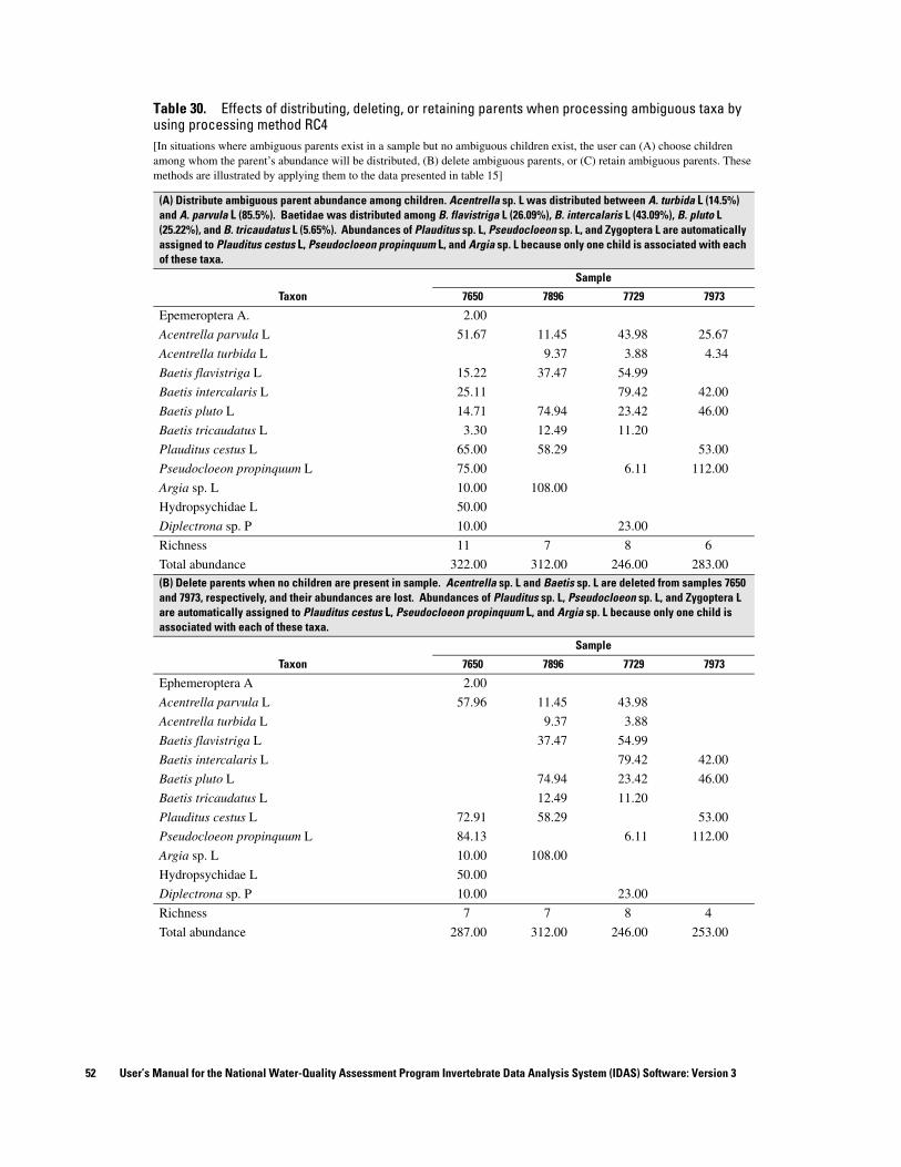
Table 30. Effects of distributing, deleting, or retaining parents when processing ambiguous taxa by using processing method RC4 [In situations where ambiguous parents exist in a sample but no ambiguous children exist, the user can (A) choose children among whom the parent’s abundance will be distributed, (B) delete ambiguous parents, or (C) retain ambiguous parents. These methods are illustrated by applying them to the data presented in table 15]

(A) Distribute ambiguous parent abundance among children. Acentrella sp. L was distributed between A. turbida L (14.5%) and A. parvula L (85.5%). Baetidae was distributed among B. flavistriga L (26.09%), B. intercalaris L (43.09%), B. pluto L (25.22%), and B. tricaudatus L (5.65%). Abundances of Plauditus sp. L, Pseudocloeon sp. L, and Zygoptera L are automatically assigned to Plauditus cestus L, Pseudocloeon propinquum L, and Argia sp. L because only one child is associated with each of these taxa.

Sample

Taxon 7650 7896 7729 7973

Epemeroptera A. 2.00

Acentrella parvula L 51.67 11.45 43.98 25.67

Acentrella turbida L 9.37 3.88 4.34

Baetis flavistriga L 15.22 37.47 54.99

Baetis intercalaris L 25.11 79.42 42.00

Baetis pluto L 14.71 74.94 23.42 46.00

Baetis tricaudatus L 3.30 12.49 11.20



Argia sp. L 10.00 108.00



Richness 11 7 8 6

Total abundance 322.00 312.00 246.00 283.00(B) Delete parents when no children are present in sample. Acentrella sp. L and Baetis sp. L are deleted from samples 7650 and 7973, respectively, and their abundances are lost. Abundances of Plauditus sp. L, Pseudocloeon sp. L, and Zygoptera L are automatically assigned to Plauditus cestus L, Pseudocloeon propinquum L, and Argia sp. L because only one child is associated with each of these taxa.

Sample

Taxon 7650 7896 7729 7973






Baetis pluto L 74.94 23.42 46.00




Argia sp. L 10.00 108.00



Richness 7 7 8 4

Total abundance 287.00 312.00 246.00 253.00


If the user elects to delete ambiguous parents in cases where there are no associated children in the sample, the IDAS program will delete the parent and its abundance before distributing the abundance of any remaining ambiguous parents among the associated children (table 30B). Similarly, if the user chooses to retain ambiguous parents in samples where there are no associated children, the IDAS program will distribute the abundance of ambiguous parents while taking the retained parents’ abundances into consideration. This will result in a processed data set that contains taxonomic ambiguities (table 30C).

The examples presented in tables 29 and 30 did not mix the distribute, delete, or retain options. This was done to simplify these examples. However, the IDAS program allows the analyst to mix these options when dealing with ambiguous parents. These actions will be applied only to the ambiguous parents that are present in a sample without associated children. The combination of these options provides the analyst with a diverse and powerful set of tools for resolving taxonomic ambiguities.

Running the Data Preparation Module

Once the user has made selections on the Data Preparation module’s main form (fig. 13), the choices can be executed by clicking on Run on the menu line at the top of the form. This action calls up the processing status window (fig. 22), which informs the user of actions the module is currently conducting (highlighted lines), actions that have been completed (overstrike lines), and actions that have not been selected (dimmed lines). At the bottom on the startup window is a list box that displays the samples that have been resolved (SUID, STAID, and SMCOD). A text box immediately above the list box provides information on the percentage of samples that have been processed. The Hide and Reset menu items at the top of this window allow the user to hide the window or to reset the contents of the window. If the Status window is hidden, it can be reactivated by clicking on the Status menu item in the main window of the Data Preparation module (fig. 13).

When processing has been completed, the Processing status window is displayed over the Data

(C) Retain parents when no children are present in a sample, otherwise distribute abundances among children. Acentrella sp. L and Baetis sp. L are retained. Abundances of Plauditus sp. L, Pseudocloeon sp. L, and Zygoptera L are automatically assigned to Plauditus cestus L, Pseudocloeon propinquum L, and Argia sp. L because only one child is associated with each of these taxa.

Sample

Taxon 7650 7896 7729 7973


Acentrella sp. L 30.00



Baetis sp. L. 58.33



Baetis pluto L 74.94 23.42 46.00




Argia sp. L 10.00 108.00



Richness 8 7 8 5

Total abundance 322.00 312.00 246.00 283.00

Table 30. Effects of distributing, deleting, or retaining parents when processing ambiguous taxa by using processing method RC4 — Continued[In situations where ambiguous parents exist in a sample but no ambiguous children exist, the user can (A) choose children among whom the parent’s abundance will be distributed, (B) delete ambiguous parents, or (C) retain ambiguous parents. These methods are illustrated by applying them to the data presented in table 15]


Figure 22. The processing status window from the Data Preparation module. The highlighted line indicates that the IDAS program is currently copying results to the output files. The dimmed lines are processing options that have not been selected.

TIP: Click on “Hide” to return to the Data Preparation window. You can then select new processing options to apply to the open data set.

preparation window (fig. 13). Click on the Hide menu item of the Processing status window to return to the Data preparation window with all the processing options preserved. A new set of sample-processing options can be applied to the open data file simply by selecting a new set of options. These options are executed, and a new “processed” data file is created by clicking on Run in the menu line. In this fashion, the user can process quantitative samples and then qualitative samples or investigate different methods of resolving taxonomic ambiguities, deleting rare taxa, or the effects of using different taxonomic levels without having to reopen the data file for each analysis.

Output from the Data Preparation Module

The IDAS program prompts the user to supply a name for the processed data that are stored by the Data Preparation module as a new data table or spreadsheet

(fig. 9) in the Access database or Excel workbook that provided the abundance data. This name must be 15 characters or less to accommodate the suffixes (up to 12 characters in length) that IDAS uses to identify output files while still meeting the 31-character limit for spreadsheet names in Excel. The default name that the IDAS program provides for the processed data is “NoAmbig.” The format of the processed data (appendix table II-1) is slightly different from that of the original data (appendix table I-1) and is arranged in order by SUID, STAID, Reach, CollectionDate, SampleID, SortCode, and Lifestage.

In addition to the processed data, this module will, depending on the processing options selected by the user, produce another two or three tables or spreadsheets that document

TIP: Output data tables and spreadsheets are automatically appended to the workbook or database that provided the data.


the data-processing steps selected by the user. These tables are stored in the database or workbook that provided the abundance data. The options table is stored under the user-supplied name plus the suffix “_Options” (for example, NoAmbig_Options). The options table documents the data preparation by storing information on the name of the source data file(s), the output data table or spreadsheet, and the options selected (appendix table II-3).

Statistics on the number of rows of data and abundance associated with each sample are calculated at three points during data processing. These statistics are stored in a table or spreadsheet named by combining the user-supplied name plus the suffix “_Stats” (for example, NoAmbig_Stats). An example of the data-preparation statistics that are output by the IDAS program is given in appendix table II-4. For each sample, the numbers of rows are given for (1) the original data (oRows); (2) after processing lab notes, lifestages, selecting lowest taxa levels, and deleting rare taxa (dRows); and (3) after resolving ambiguities (aRows). Total abundances at each processing stage are stored in the columns oAbund, dAbund, and aAbund (or oDensity, dDensity, and aDensity — if the “calculate density” option was chosen). These statistics give insight into how much the information content of the data changes as these samples are prepared for analysis.

If the user chooses to form QUAL samples from compilations of RTH, DTH, and QMH samples, the IDAS program will store information on which RTH and DTH samples are paired with which QMH samples. It will also store a list of the SampleID’s and SMCOD’s that are created to identify the QUAL sample. All of this information is stored in a new spreadsheet or data table that is named by combining the user-supplied name with the suffix “_QQsmcods” (for example, NoAmbig_QQsmcods; appendix table II-2).

Resetting or Exiting the Module

The user can reset the module by selecting the Close option from the Files menu. This will return the user to the opening window of the module and prepare the module to open a new data set. This is the procedure to follow if the user wishes to process multiple data sets through the same module. The user can exit the module by selecting Exit from the menu bar. This will close the module and return the user to the opening screen of the IDAS program (fig. 1). Alternatively, the user can click on the “x” in the upper right-hand corner of the window. To apply different processing options to the same data set, the user does not have to close and reopen the file for

processing but simply can click on the Hide menu item on the Processing status window and then select the desired processing options on the Data Preparation window and click on Run to process the data.

CALCULATE COMMUNITY METRICS MODULE

The Calculate Community Metrics module calculates more than 130 community metrics (appendix table III-1). This module is started by clicking on the Calculate community metrics button on the main program window (fig. 1). This module uses the “processed” data format (appendix table II-1) produced by the Data Preparation module. It will not accept data in Bio-TDB format (appendix table I-1) because this module assumes that each row in a sample corresponds to what the user has decided is a unique taxon (BU_ID or BU_ID + lifestage). This module (fig. 23) uses standard menu items for opening and closing files (Files), viewing data files (View), exiting the module (Exit), displaying information about the module (About), and for executing selected processing options (Run). The View menu also can be used to view and print a list of the community metrics calculated by this module. A standard five-panel status bar located along the bottom of the module window displays (from left to right) the name of the source file, the source file type (Excel or Access), the name of the spreadsheet or data table that is the source of the data, the name of the spreadsheet or data table that will store the processed data, and processing status messages.

The Calculate Community Metrics module derives metrics based on taxa richness, abundance, tolerance, trophic groups, and functional groups. This module allows the user to calculate the following:

1. Richness metrics: 25 metrics based on the number of taxa.

2. Percent richness metrics: 24 metrics based on the percentage of total richness.

3. Abundance metrics: 25 metrics based on abundance of taxa.

4. Percent abundance metrics: 24 metrics based on percentage of total abundance.

5. Tolerance metrics: average tolerance based on richness and abundance.

TIP: The Calculate Community Metrics module uses the “processed” data format produced by the Data Preparation module.

Calculate Community Metrics Module 55

Figure 23. Main window of the Calculate Community Metrics module. The “Select metrics” frame appears after the user has opened an Excel spreadsheet or Access table for processing.

6. Functional group metrics: 32 metrics based on richness, percentage richness, abundance, and percentage abundance of taxa in 8 functional groups.

7. Dominance metrics: 5 metrics showing the percentage of total abundance represented by the most abundant taxon, two most abundant taxa, three most abundant taxa, four most abundant taxa, and five most abundant taxa.

Processing Options

Once the user successfully opens a data file by using the Files/Open menus, the Select metrics frame appears on the main window of the Calculate Community Metrics module (fig. 23). This frame allows the user to select various richness metrics, abundance metrics,

tolerance metrics, and functional group metrics (appendix table III-1). The IDAS program automatically checks to see if the input data contain quantitative samples (RTH and(or) DTH samples); if none are detected, the metrics requiring quantitative data are disabled (dimmed). If the data set contains both quantitative (RTH, DTH) and qualitative (QUAL, QMH) samples, the user can select the quantitative metrics even though these metrics cannot be calculated for qualitative samples. When the IDAS program encounters a situation in which it cannot calculate a metric (for example, calculating a quantitative metric for a qualitative sample), it will assign a null (Access tables) or blank (Excel spreadsheets) value to the metric. Although this module can handle mixed data sets (qualitative and quantitative), it is strongly recommended that qualitative and quantitative samples be analyzed separately.


Richness and abundance metrics are derived from aggregations of abundance or richness data by using the taxonomic information contained in the data set (for example, EPT richness is the count of rows of data in a sample where the column “order” contains the values “Ephemeroptera,” “Plecoptera,” or “Trichoptera;” EPT abundance is the sum of abundances for these orders). Tolerance and functional feeding group metrics are based on data derived from appendix B of the U.S. Environmental Protection Agency’s (USEPA) Rapid Bioassessment Protocol (RBP) (Barbour and others, 1999). The RBP provides regional tolerances and a primary and secondary functional group for a large number of taxa. The IDAS program stores this information in the spreadsheet Attrib (appendix table III-2) of the Excel file Attributes.xls. This file is installed in the same directory as the IDAS program during the installation of IDAS. The national tolerance values stored in Attrib are the average of regional tolerance values reported in appendix B of the RBP. Functional feeding group metrics are formed by counting the number of rows (for example, PR_rich) in each sample that correspond to the eight functional feeding group abbreviations (appendix table III-1) or summing the abundances (for example, PR_abund) that correspond to these abbreviations. The tolerance metrics are calculated as the average tolerance value of all taxa in a sample (RichTOL) or by weighting the tolerance value by the abundance of the organism in the sample (AbundTOL).

(1)

(2)

where TVi is the USEPA tolerance value for taxon “i” Ai is the abundance of taxon “i” in the sample n is the number of taxa in the sample N is the total abundance in the sample

Unfortunately, the format of the names of taxa in the RBP and Bio-TDB do not match because the RBP

does not include authority names. For this reason, the IDAS program uses a taxonomic equivalency table (spreadsheet EQTX in Attributes.xls) to relate Bio-TDB BU_ID’s to the names listed in the RBP (appendix table III-3). Names are matched by using one of two methods: (1) direct matching and (2) maximum equivalency. The direct-matching method involves removing the authority name from the Bio-TDB BU_ID to create the column “Name” in EQTX and then matching these names to those used by the USEPA. The maximum-equivalency method involves matching a list of equivalent names for tolerance (column “EQTXTOL”) or functional feeding groups (column “EQTXFG”) to the names used by the USEPA.

The lists of equivalent names are designed to maximize the correspondence between the Bio-TDB BU_ID’s and the USEPA names for tolerance and functional feeding group data. If a direct match does not exist for a BU_ID in the USEPA data, a match is sought by setting the BU_ID to the next highest taxonomic level. This is repeated until a match is found or the level of phylum is reached. This approach maximizes the number of matches between the Bio-TDB and USEPA taxa lists, but it assumes that the tolerances and functional feeding groups reported at higher taxonomic levels are applicable to the aggregation of data from lower levels. The IDAS program keeps track of the percentage of taxa (data rows) and abundance that are matched with USEPA tolerance and functional group data.

A pop-up window (fig. 24) allows the user to select how Bio-TDB names are matched with USEPA names and, for tolerance data, whether to use a regional tolerance list or the national list (appendix table II-3). Selecting Taxa name without authority invokes the direct-matching method. Selecting Equivalent taxa name invokes the maximum-equivalency method. The analyst should pay particular attention to the statistics that IDAS provides (“_class”) on the percentage of taxa richness and abundance that are assigned functional groups or tolerance values in this module. If the percentage that is classified is low (less than 80 percent), the analyst should be concerned that these metrics may not adequately represent the community.

RichTOL Σ TVi( ) n⁄=

AbundTOL Σ TVi( ) Ai( )×( ) N⁄=

Calculate Community Metrics Module 57

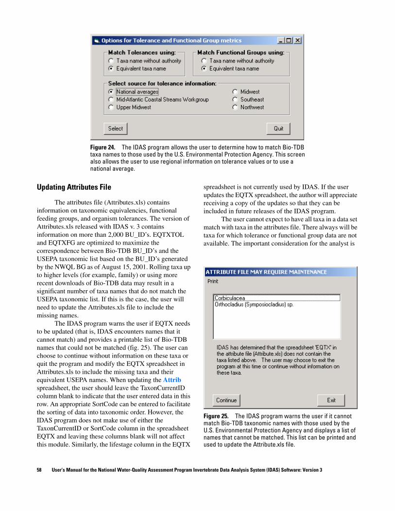
Figure 24. The IDAS program allows the user to determine how to match Bio-TDB taxa names to those used by the U.S. Environmental Protection Agency. This screen also allows the user to use regional information on tolerance values or to use a national average.

Updating Attributes File

The attributes file (Attributes.xls) contains information on taxonomic equivalencies, functional feeding groups, and organism tolerances. The version of Attributes.xls released with IDAS v. 3 contains information on more than 2,000 BU_ID’s. EQTXTOL and EQTXFG are optimized to maximize the correspondence between Bio-TDB BU_ID’s and the USEPA taxonomic list based on the BU_ID’s generated by the NWQL BG as of August 15, 2001. Rolling taxa up to higher levels (for example, family) or using more recent downloads of Bio-TDB data may result in a significant number of taxa names that do not match the USEPA taxonomic list. If this is the case, the user will need to update the Attributes.xls file to include the missing names.

The IDAS program warns the user if EQTX needs to be updated (that is, IDAS encounters names that it cannot match) and provides a printable list of Bio-TDB names that could not be matched (fig. 25). The user can choose to continue without information on these taxa or quit the program and modify the EQTX spreadsheet in Attributes.xls to include the missing taxa and their equivalent USEPA names. When updating the Attrib spreadsheet, the user should leave the TaxonCurrentID column blank to indicate that the user entered data in this row. An appropriate SortCode can be entered to facilitate the sorting of data into taxonomic order. However, the IDAS program does not make use of either the TaxonCurrentID or SortCode column in the spreadsheet EQTX and leaving these columns blank will not affect this module. Similarly, the lifestage column in the EQTX

spreadsheet is not currently used by IDAS. If the user updates the EQTX spreadsheet, the author will appreciate receiving a copy of the updates so that they can be included in future releases of the IDAS program.

The user cannot expect to have all taxa in a data set match with taxa in the attributes file. There always will be taxa for which tolerance or functional group data are not available. The important consideration for the analyst is

Figure 25. The IDAS program warns the user if it cannot match Bio-TDB taxonomic names with those used by the U.S. Environmental Protection Agency and displays a list of names that cannot be matched. This list can be printed and used to update the Attribute.xls file.


what proportion of taxa richness and abundance are assigned values from the attributes file. The IDAS program assists the analyst in this effort by providing statistics on the percentages of taxa richness and abundance that are assigned functional-group (FG_RICH_class, FG_ABUND_class) and tolerance (RICH_TOL_class, ABUND_TOL_class) values (appendix table III-1). The analyst is advised to be concerned about using tolerance or functional-group metrics if the percentage of taxa richness or abundance that is assigned a value falls below 80 percent or if there is a wide disparity among samples in the classification (_class) metrics.

Output From the Module

The Calculate Community Metrics module can generate up to seven new spreadsheets or tables that are stored in the source Excel workbook or Access database. Spreadsheet or data table names are formed by appending suffixes to the name of the spreadsheet or data table from which the input data were derived (table 31). Each output data table or spreadsheet includes SUID, STAID, Reach, CollectionDate, SampleID, SMCOD, and the metrics as columns. The list of metrics in each output Access data table or Excel spreadsheet is given in appendix table III-1.


The user can reset the module by selecting the Close option from the Files menu. This returns the user to the opening window of the module and prepares the module to accept a new data set. This is the procedure to follow if the user wishes to process multiple data sets

through the same module. The user can exit a module by selecting Exit from the menu bar. This closes the module and returns the user to the opening screen of the IDAS program (fig. 1). The user also can exit the module by clicking on the “x” in the upper right-hand corner of the module window.

CALCULATE DIVERSITIES AND SIMILARITIES MODULE

The Calculate Diversities and Similarities module uses Excel spreadsheets or Access data tables produced by the Data Preparation module (appendix table II-1) to calculate five diversity indices, three evenness indices, one dominance index, and eight similarity indices (appendix table IV-1). This module will not accept data in Bio-TDB format (appendix table I-1). Descriptions, equations, and references for calculating the diversity indices are given in appendix table IV-2 and in appendix table IV-3 for similarity indices.

Clicking on the Calculate Diversities and Similarities button in the main program window (fig. 1) will start this module and display the Calculate diversity and similarity indices module window (fig. 26). This module uses standard menu items for opening and closing files (Files), viewing data files (View), executing selected processing options (Run), exiting the module (Exit), and displaying information about the module (About). The module has a standard five-panel status bar that displays (from left to right) the name of the source file, the source-file type (Excel or Access), the name of the spreadsheet or data table that is the

source of the data, the name of the spreadsheet or data table that will store the processed data, and processing status information.

Table 31. Output tables that can be produced by the Calculate Community Metrics module [The data originated from a data table or spreadsheet named “ALMN”]

Name Description

ALMN_R_Metrics Richness metrics

ALMN_pR_Metrics Percentage richness metrics

ALMN_A_Metrics Abundance metrics

ALMN_pA_Metrics Percentage abundance metrics

ALMN_DOM_Metrics Dominance metrics

ALMN_FG_Metrics Functional group metrics, richness and abundance

ALMN_TOL_Metrics Tolerance metrics, richness and abundance

TIP: The Calculate Diversities and Similarities module uses the “processed” data format produced by the Data Preparation module.

TIP: Diversity and similarity indices should be calculated separately for qualitative and quantitative samples.

Calculate Diversities and Similarities Module 59

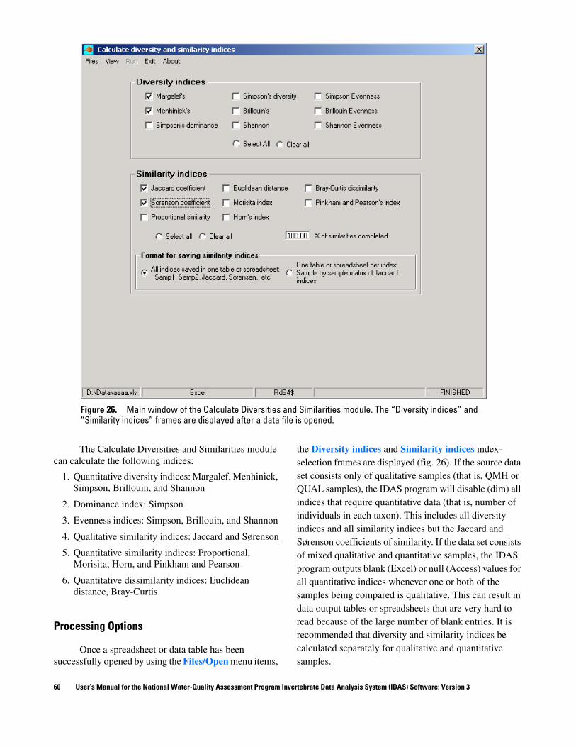
Figure 26. Main window of the Calculate Diversities and Similarities module. The “Diversity indices” and “Similarity indices” frames are displayed after a data file is opened.

The Calculate Diversities and Similarities module can calculate the following indices:

1. Quantitative diversity indices: Margalef, Menhinick, Simpson, Brillouin, and Shannon

2. Dominance index: Simpson

3. Evenness indices: Simpson, Brillouin, and Shannon

4. Qualitative similarity indices: Jaccard and Sørenson

5. Quantitative similarity indices: Proportional, Morisita, Horn, and Pinkham and Pearson

6. Quantitative dissimilarity indices: Euclidean distance, Bray-Curtis

Processing Options

Once a spreadsheet or data table has been successfully opened by using the Files/Open menu items,

the Diversity indices and Similarity indices index-selection frames are displayed (fig. 26). If the source data set consists only of qualitative samples (that is, QMH or QUAL samples), the IDAS program will disable (dim) all indices that require quantitative data (that is, number of individuals in each taxon). This includes all diversity indices and all similarity indices but the Jaccard and Sørenson coefficients of similarity. If the data set consists of mixed qualitative and quantitative samples, the IDAS program outputs blank (Excel) or null (Access) values for all quantitative indices whenever one or both of the samples being compared is qualitative. This can result in data output tables or spreadsheets that are very hard to read because of the large number of blank entries. It is recommended that diversity and similarity indices be calculated separately for qualitative and quantitative samples.


Output From the Module

Output from the Calculate Diversities and Similarities module is stored in new spreadsheets or data tables within the Excel workbook or Access database that was the source for the input data. These new spreadsheets or data tables are named by appending an appropriate suffix to the name of the spreadsheet or data table that was the source of the data. For example, if the data originate from an Excel spreadsheet called “ALMN,” then all diversity indices will be stored in a new spreadsheet called “ALMN_Diversity.” This module can produce from 1 to 9 new spreadsheets or tables depending upon the options chosen by the user (appendix table IV-4).

All diversity indices are stored in one spreadsheet or data table (appendix table IV-5). However, this module gives the user the option to save all similarity indices into a single table or to save each similarity index into a separate table. When similarity indices are stored in a single table, each row corresponds to a couplet of samples and the columns correspond to the similarity indices selected by the user (appendix table IV-6). This method of presentation is useful when the analyst is most interested in comparing differences among similarity indices rather than comparing differences in similarities among samples. Because each column corresponds to a similarity index and each row to a two-sample comparison, it is very easy to pull these data into a spreadsheet and calculate statistics that compare similarity indices (columns). However, having the rows correspond to pairs of samples makes it difficult to determine how similar samples are to one another.

Saving each similarity index to a separate table produces a symmetric matrix of similarity values in which each column compares a sample to all other samples (appendix table IV-7). This format is very useful if the objective is to understand how similar samples are to one another rather than how different similarity indices compare to one another. However, if the matrix of similarities contains large numbers of blank values, which happens when analyzing mixed quantitative and qualitative data, then the symmetric matrix of similarities can be difficult to view. Therefore, it is recommended that qualitative and quantitative samples be analyzed separately unless there is a compelling reason to analyze them together. Also, Excel and Access have limitations on the number of columns of data that can be stored in a spreadsheet or data table. It is relatively easy to exceed these limits (about 256 columns) using this format.


The IDAS program indicates that the module has finished calculating and saving diversity and similarity indices by displaying the word FINISHED in the right-hand panel of the status bar (fig. 26). The user may reset the module and process another data set by selecting File/Close from the menu bar. Clicking on Exit on the menu bar will shut down this module and return the user to the main IDAS window (fig. 1). The user also can exit this module by clicking on the “x” in the upper right-hand corner of the module window.

DATA EXPORT MODULE

The Data Export module uses spreadsheets or tables produced by the Data Preparation module (appendix table II-1) to produce ASCII text files that can be imported into spreadsheets (for example, Excel), databases (for example, Access), statistical packages (for example, SYSTAT, S-PLUS, SAS, CANOCO, TWINSPAN), and graphics packages (for example, CorelDraw). This module also produces a site (columns) by taxa (rows) table that can be used to publish invertebrate community data in reports. The Data Export module will not accept data in Bio-TDB format (appendix table I-1).

The Data Export module is activated by clicking on the Data Export button of the main IDAS window (fig. 1). This brings up the Format data for export window (fig. 27). This module uses standard menu items for opening and closing files (Files), viewing data files (View), executing selected processing options (Run), exiting the module (Exit), and displaying information about the module (About). The bottom of the module has a standard five-panel status bar that displays (from left to right) the name of the source file, the source-file type (Excel or Access), the name of the spreadsheet or data table that is the source of the data, the name of the spreadsheet or data table that will store the processed data, and processing status messages.

This module can export data as abundance, density, proportions (abundance and density), and percentages (abundance and density). These data can be exported in three formats:

1. Comma-delimited ASCII files

A. Samples as rows, taxa as columns

B. Taxa as rows, samples as columns

2. Tab-delimited ASCII files (taxa as rows) with full sample and taxonomic information

3. CANOCO-condensed format

Data Export Module 61

Figure 27. Main window of the Export Data module. The frames “Export data as” and “Export data format” appear after the user successfully opens a spreadsheet or data table using the Files/Open menu items.

Processing Options

Processing begins by clicking on the Files/Open menu items and selecting an Excel spreadsheet or Access table containing invertebrate abundance or density data. Once a spreadsheet or data table has been successfully opened, the selection frames Export data as and Export data format will appear (fig. 27). The Export data as frame allows the user to convert abundance or density data to percentages (0 – 100%) or proportions (0 – 1).

The IDAS program does not differentiate between qualitative and quantitative samples when calculating percentages or proportions in the Export Data module. If the user elects to calculate percentages or proportions

on a data set containing qualitative samples, the resulting values will be identical for all taxa within a qualitative sample because all taxa in a qualitative sample are assigned an abundance or density value of one (1). Consequently, the values obtained for qualitative samples depend on the number of taxa in the sample rather than on abundance. For this reason, it is recommended that percentages and proportions not be calculated for data sets that contain qualitative samples.

The Export data format frame allows the user to select a format for the text files produced by this module. Files may be exported as comma-delimited ASCII, tab-delimited ASCII, or as CANOCO native format. The comma-delimited ASCII formats are compatible with many common software packages, including SYSTAT, S-PLUS, Access, and Excel. Data can be exported with rows as samples and columns as taxa (appendix

TIP: Do not convert qualitative data to percentages or proportions.


table V-1) or with rows as taxa and columns as samples (appendix table V-2), depending on the needs of the user and the characteristics of the software. Some software programs (for example, Excel) have limitations on the number of rows and(or) columns that can be imported. Because expressing taxa as rows or columns affects the number of rows and columns in the resulting file, it also may affect whether the software program can import the resulting file. For example, appendix tables V-1 and V-2 contain exactly the same data. However, appendix table V-1 cannot be imported into Excel because the taxa are stored in 339 columns, which exceeds the number of columns (256) that Excel can import. Appendix table V-2 has samples stored in just 67 columns, so this table can be imported into Excel even though it contains just as many cells as appendix table V-1.

Comma-delimited and CANOCO native formats use simple abbreviations to represent the names of taxa and samples (appendix table V-1). Abbreviations are used because some software programs (for example, CANOCO and SAS) require variable names to be eight characters or less. When the IDAS program uses abbreviations, it produces a “key” file that contains a list

of abbreviations, the information represented by the abbreviations, the text file to which the abbreviations apply, the date and time that the text files were created, and the name and path of the Excel or Access file that supplied the data (appendix

table V-3). “Key” files are named by adding the suffix “_key” to the name used to store the exported abundance or density data. For example, if the user elects to store data for the ALMN Study Unit in a file named “ALMN.txt,” the IDAS program provides “ALMN_key.txt” as the default name for the “key” file. The user has the option of changing the default name provided by IDAS, but this will make it more difficult to associate the exported data with the list of abbreviations. Even if the user changes the name of the “key” file, the abbreviations still can be associated with the exported file because the “key” file contains the name of the text file to which the abbreviations apply and the name of the Excel or Access file from which the data were originally derived (appendix table V-3).

The tab-delimited, full format option is provided to help with the process of creating data tables for reports or other purposes in which abbreviations are not appropriate. This option exports data with taxa as rows and samples as columns (appendix table V-4). The rows of taxa data are sorted in phylogenetic order and contain all taxa levels from phylum to BU_ID as well as lifestage and SortCode data. The columns of data are identified as SUID, STAID, Reach, CollectionDate, SampleID, and SMCOD. The column header also indicates what the data represent — abundance (Abundance), density (Density), proportions of abundance (Prop_Abundance), proportions of density (Prop_Density), percentages of abundance (%_Abundance), or percentages of density (%_Density). This format, when imported into Excel, provides an easy way to view and compare data sets.

The CANOCO native format option produces a file in Cornell Ecology Package (CEP) condensed format (appendix table V-5). The CEP-condensed format produces a very compact data file that was developed in the 1970’s when computer analysis relied on Fortran and punched cards. Despite the antiquity of this format, it still is used by several important software packages that are the standards for community ordinations. The files produced by this option will work with the DOS® and Windows® versions of CANOCO, MVSP, and PC-ORD, and the DOS version of CEP (including TWINSPAN), MVSP, and PC_ORD. CANOCO native format files are stored with the extension *.cnd to distinguish them from the other comma- and tab-delimited text files (*. txt) created by the Data Export module.

The CANOCO-condensed file format begins with a header line (maximum of 80 characters) that identifies the file contents. The IDAS program prompts the user to enter a title line or to accept the default header line provided by IDAS (fig. 28). The CANOCO native format option uses abbreviations for taxa and sample names because the CANOCO program has an eight-character restriction on variable names. As in other cases where

TIP: The tab-delimited, full format option is very useful for examining community data or generating reports for publication.

Figure 28. The IDAS program prompts the user to supply a header line for files stored in CANOCO native format files.

Data Export Module 63


IDAS uses abbreviations, this option produces a “key” file that contains a list of the abbreviations, the information represented by the abbreviations, the file associated with these abbreviations, and the name and path of the Excel or Access file that provided the original data. The “key” file is stored with the same *.cnd extension that is used to store the data. Assuming that the user chooses to store the data in a file named “ALMN.cnd,” the IDAS program will use “ALMN_key.cnd” as the default name for the “key” file.

Duplicate Sort Codes

Sort codes (SortCode) in Bio-TDB are not static; they change over time as new taxa are added to the master taxa list maintained by the NWQL BG. Consequently, it is possible to introduce duplicate sort codes into IDAS data sets by combining data (for example, data from multiple Study Units) that were downloaded from Bio-TDB at different times. The IDAS program addresses this problem by checking files for duplicate sort codes every time if opens a data file. If the IDAS program finds duplicate sort codes, it will warn the user and provide a list of taxa that have duplicate codes (fig. 29). Duplicate sort codes do not affect the Edit Data, Data Preparation, Calculate Community Metrics, or Calculate Diversities and Similarities modules. These modules check for the presence of duplicate sort codes and warn the user if any are found. When these modules process data sets, however, they eliminate duplications by selecting the maximum value of the sort codes associated with each taxon (BU_ID or BU_ID + lifestage). Duplicate sort codes are a problem only in the Data Export module where they

can produce multiple lines of data for a single taxon and corrupt the taxonomic order. If the Data Export module detects duplicate sort codes, the user will need to manually check the resulting table and fix any problems with duplicate entries or taxa that are not in phylogenetic order. While it is possible to produce data sets with multiple sort codes, the algorithms built into the IDAS program should ensure that this will be an infrequent occurrence.


The IDAS program indicates that the module has finished calculating and saving diversity and similarity indices by displaying the word FINISHED in the right-hand panel of the status bar. The user may reset the module and process another data set by selecting File/Close from the menu bar. Clicking on Exit on the menu bar will shut down this module and return the user to the main IDAS window (fig. 1). The user also may exit this module by clicking on the “x” in the upper right-hand corner of the module window.

TROUBLESHOOTING

The IDAS program has been tested on a variety of computers running different versions of Windows (NT, 2000, XP) and Microsoft Office® under a variety of computing environments typically found in USGS and home offices. Numerous data-checking and error-trapping subroutines have been built into the program in an effort to detect problems before they affect the program or to deal with problems after the program detects them. This section describes the various error-handling procedures built into the IDAS program and what to do when the program abnormally terminates.

Types of Errors

The IDAS program has been designed to handle various situations where errors may arise. Errors can be divided into three categories: anticipated, unanticipated but trappable, and unanticipated and untrappable. Anticipated errors are those that normally arise from inappropriate action by the user. This includes selecting files with the wrong formats, selecting combinations of options that generate no data, or saving data to spreadsheets or data tables that already exist. The IDAS program includes subroutines that detect these errors, alert the user that an error has occurred, and provide an opportunity to correct the error (fig. 30).

Figure 29. The IDAS message box that alerts the user of the presence of duplicate sort codes in the data.

Unanticipated but trappable errors can occur when a file selection, query, or calculation generates a system error. For example, division by zero generates an error, as does trying to open a file that is already in use by another program. The IDAS program traps these errors and reports them back to the user (fig. 31). These errors generate an error message window that includes a header that tells where the error occurred in the program (for example, Calculate Diversities and Similarities module), the error number used by Visual Basic (#3075), and a brief description of the error (a syntax error in a query). When a trappable error is encountered, it is important for the user to copy down all information included in the error message and report it to the author as soon as possible.

The user should also include a complete description of what was being done when the error occurred, the data file that caused the error, and the options that were selected (see Reporting Program Bugs).

Unanticipated and untrappable errors usually occur when a conflict arises between the IDAS program and another program. For example, opening Excel and attempting to read a data file that is being processed by the IDAS program will generate errors in Excel that affect the IDAS program but cannot be detected by the IDAS program. This type of error can cause the IDAS program to terminate abnormally (see Abnormal Termination). These types of errors will be extremely rare. If they occur, however, the user should notify the author as soon as possible and provide a description of what happened, what programs were being used, the IDAS options that were selected, and the data file that was being used. This type of error occurs most often when system resources (for example, memory and hard disk space) are low. Keeping the size of the Excel workbooks small and keeping as few applications open as possible will help reduce errors related to resource problems.

Error Messages

The IDAS program can generate a large number of error messages of the type described in figure 31. The 45 most common error messages are listed alphabetically in appendix VI. This list includes a description of the error message, its probable cause, and the actions that the user should take to resolve the error.

Reporting Program Bugs

A program bug may be a calculation that does not appear to be correct, a problem with formatting output, user messages or interfaces that are not intuitive, or some other problem that interferes with the use of the IDAS program. If the user encounters a bug in the IDAS

program; it should be reported to the program author as soon as possible. Please provide a complete description of the problem, any error messages that were displayed, a copy of the data file that was being processed, and a list of options that were selected.

Figure 30. Error message generated by an anticipated and trappable error. This type of error message describes the error and lists the variable(s) that produced the error so the user can correct the problem that is causing the error. In this example, the program detected missing values in the CollectionDate column.

Figure 31. Error message generated by an unanticipated but trappable error. In this example, a missing data value caused an error in a database query.

Troubleshooting 65

Abnormal Termination of IDAS

The IDAS program has been designed to trap errors and gracefully exit the module where the error occurred. However, it is not possible to anticipate all potential sources of error. Therefore, on rare occasions, the IDAS program may terminate abnormally. Abnormal termination occurs when the IDAS program terminates without the user clicking on the “Exit” button from the opening window (fig. 1). If the IDAS program terminates abnormally, it is possible that it will leave a hidden copy of Excel running and the source data file open. This will prevent the user from accessing the data file by using another copy of Excel because the data will already be in use. If the IDAS program terminates abnormally, the MS Task Manager® can be used to see if a copy of Excel (EXCEL.EXE) or IDAS (IDAS.EXE) is still running. If this occurs, these programs should be closed. But first, make sure that any other copies of Excel that may be running are closed because Task Manager will not be able to distinguish between the hidden and visible copies of EXCEL.EXE. Abnormal termination also will leave a temporary Access file on the user’s computer. This file (T%%%Temp.mdb) will be located in the directory that was the source of the invertebrate abundance data spreadsheet or data table. The IDAS program will automatically delete this file the next time it processes a data file from this directory, so the user does not need to remove this file manually.

SUMMARY

The Invertebrate Data Analysis System (IDAS) program provides an accurate, consistent, efficient, and user-friendly mechanism for analyzing invertebrate data collected as part of the National Water-Quality Assessment (NAWQA) Program and for exporting data to other computer programs. The IDAS program provides standardized tools to capture, edit, analyze, and export data downloaded from the NAWQA Program’s Biological Transactional Database (Bio-TDB). The format of data exported from Bio-TDB is optimized for efficient storage and must be manipulated before it can be imported into other data analysis software packages or into tables for publication. The IDAS program provides the tools to accomplish these manipulations and to access a variety of ecological data needed to calculate tolerance and functional group metrics. This software package reads and writes data files in the Microsoft Excel® format

exported by Bio-TDB or, for faster performance, Microsoft Access® versions of these Excel files.

The IDAS program consists of five modules — Edit Data, Data Preparation, Calculate Community Metrics, Calculate Diversities and Similarities, and Data Export modules. The Edit Data module allows the user to subset data into new spreadsheets or tables based on sample (combinations of SUID, STAID, Reach, CollectionDate, SampleID, SMCOD, or SampleType) or taxonomic information (for example, major orders of insects, major families of Diptera). This module is capable of combining spreadsheets or tables with similar formats into new spreadsheets or tables and deleting spreadsheets or tables of any type. The Edit Data module also summarizes the distribution of taxa in a data file. It identifies which taxa in a data set are ambiguous (that is, data are reported for a lower taxonomic level) in the data set, counts the number of ambiguous children associated with each ambiguous taxon, sums the abundances of the ambiguous children, and calculates the percentage of total abundance composed of these children. It also reports the number of sites where the taxon is found, the number of samples containing the taxon, the abundance of the taxon, and basic statistics (mean, maximum, minimum, and standard deviation) for taxon abundance across all samples and across only samples in which the taxon occurs. The Edit Data module is the only IDAS module that processes data files downloaded from Bio-TDB and data files produced by the Data Preparation module.

The Data Preparation module prepares data for analysis. This module processes data exported from Bio-TDB and produces a new “processed” format that can be read by the other IDAS modules. The Data Preparation module allows the user to select the type of samples to process (RTH, DTH, QMH, and(or) QUAL), calculates densities (no./m2), deletes taxa based on laboratory processing notes, deletes or retains lifestage information, sets a lowest taxonomic level for analysis, deletes rare taxa based on number of sites where the taxon occurs and(or) the percentage abundance of the taxon in each sample, and resolves taxonomic ambiguities by using one of four methods based on separate analyses for each sample or an analysis of the combined data set. Ambiguous taxa need to be resolved prior to calculating other metrics, because the redundant taxonomic information represented by ambiguous taxa can adversely affect the calculation of richness and abundance metrics and indices. The Data Preparation module is self-documenting and stores processed data in the spreadsheet or data table that provided the Bio-TDB data. This module also produces a synthetic sample (QUAL) that


represents a list of taxa found in QMH, RTH, and(or) DTH samples collected at a site within a user-specified number of days (± 7 days) from the QMH collection date.

The Calculate Community Metrics module uses data produced by the Data Preparation module. The Calculate Community Metrics module calculates 25 metrics based on taxa richness; 24 metrics based on percentage of taxa richness; 25 metrics based on abundance or density; 24 metrics based on percentage of abundance or density; average tolerance metrics based on richness and(or) abundance; 32 functional group metrics based on richness, percentage richness, abundance or density, and percentage abundance or density; and 5 dominance metrics. This module uses an ecological attribute file (Attributes.xls) that contains data on functional feeding groups, regional ecological tolerances, and a national tolerance value that is the average of the regional values. The IDAS program allows the user to calculate tolerance values based on national or regional tolerance values. The attribute file also contains a list of equivalent taxa that allows the user to substitute functional feeding group or tolerance values reported at higher taxonomic levels (for example, genus instead of species) when a value is not available at a lower level (for example, substitute data for Hydropsyche when data are unavailable for Hydropsyche sparna). The metrics produced by this module are stored as separate spreadsheets or data tables in the workbook or database that provided the abundance data.

The Calculate Community Diversities and Similarities module uses data files produced by the Data Preparation module. This module can calculate five diversity indices (Margalef, Menhinick, Simpson, Brillouin, and Shannon), a dominance index (Simpson), three measures of evenness (Simpson, Brillouin, and Shannon), two qualitative similarity indices (Jaccard and Sørenson), four quantitative similarity indices (Proportional, Morisita, Horn, and Pinkham and Pearson), and two quantitative dissimilarity indices (Euclidean distance and Bray-Curtis). Similarity and dissimilarity indices can be saved in one of two ways: (1) in a single data table or spreadsheet with rows corresponding to sample pairs and columns to indices or (2) in a data table for each selected indices with rows and columns corresponding to sample pairs. The latter format produces a symmetric matrix with the lower half populated with the similarity indices. Results from this module are stored as separate spreadsheets or tables in the workbook or database that provided the invertebrate data.

The Data Export module uses data files produced by the Data Preparation module. The Data Export module

produces ASCII text files in comma-delimited, tab-delimited, or CANOCO-condensed formats that can be imported into other statistical packages or word-processing programs. Data can be exported in their original format (that is, abundance or density) or converted to relative abundance or density (0 – 100 percent) or proportions of abundance or density (0 – 1) and exported. Comma-delimited and CANOCO-condensed format files produce two output files: (1) a data file that contains the data (that is, abundance, density, or presence) with abbreviations (eight-characters or less) for taxa and sample names and (2) a “key” file that contains a list of the abbreviations and the full sample information and taxa names. A header in the “key” file stores the name of the data file produced by the Data Export module, the time and date that the file was created, and the name and path of the spreadsheet or data table from which the data originated. This ensures that the source and data export (data and key) can be easily associated and archived. Data also can be exported as full-format tab-delimited ASCII files with rows containing taxa and columns corresponding to samples. This format is intended to provide a table that can be imported into a word processor for publication. This format contains the full taxonomic hierarchy reported for each taxon, the taxonomic sort code, and the lifestage. Each column contains sample identification information (SUID, STAID, Reach, CollectionDate, SampleID, SMCOD, and the units of measurement [abundance or density]). The rows of taxonomic data are sorted in phylogenetic order.

REFERENCES CITED

Barbour, M.T., Gerritsen, J., Snyder, B.D., and Stribling, J.B., 1999, Rapid bioassessment protocols for use in streams and wadeable rivers — periphyton, benthic macroinvertebrates, and fish (2d ed.): U.S. Environmental Protection Agency, Office of Water, Washington, D.C., EPA 841-B-99-002.

Brower, J.E., and Zar, J.H., 1984, Field and laboratory methods for general ecology (2d ed): Dubuque, Iowa, Wm. C. Brown Publishers, p. 226.

Cao, Y., Larsen, D.P., and Thorne, R. St-J., 2001, Rare species in multivariate analysis for bioassessment — some considerations: Journal of the North American Benthological Society, v. 20, no. 1, p. 144 – 153.

Cao Y., and Williams, D.D., 1999, Rare species are important for bioassessment — reply to Marchant’s comments: Limnology and Oceanography, v. 44, p. 1841 – 1842.

References Cited 67

Cao Y., Williams, D.D., and Williams, N.E., 1998, How important are rare species in aquatic community ecology and bioassessment?: Limnology and Oceanography, v. 43, p. 1403 – 1409.

Cuffney, T.F., Gurtz, M.E., and Meador, M.R., 1993, Methods for collecting benthic invertebrate samples as part of the National Water-Quality Assessment Program: U.S. Geological Survey Open-File Report 93-406, 66 p.

Faith, D.P., and Norris, R.H., 1989, Correlation of environmental variables with patterns of distribution and abundance of common and rare freshwater macroinvertebrates: Biological Conservation, v. 50, p. 77 – 98.

Gilliom, R.J., Alley, W.M., And Gurtz, M.E., 1995, Design of the National Water-Quality Assessment Program — Occurrence and distribution of water-quality conditions: U.S. Geological Survey Circular 1112, 33 p.

Goff, F.G., 1975, Comparison of species ordinations resulting from alternative indices of interspecific association and different numbers of included species: Vegetatio, v. 31, p. 1 – 14.

Hirsch, R.M., Alley, W.M., and Wilber, W.G., 1988, Concepts for a National Water-Quality Assessment Program: U.S. Geological Survey Circular 1021, 42 p.

Leahy, P.P., Rosenshein, J.S., and Knopman, D.S., 1990, Implementation plan for the National Water-Quality Assessment Program: U.S. Geological Survey Open-File Report 90-174, 10 p.

Marchant, R., 1990, Robustness of classification and ordination techniques applied to macroinvertebrate communities from the La Trobe River, Victoria: Australian Journal of Marine and Freshwater Research, v. 41, p. 493 – 504.

Marchant, R., Hirst, A., Norris, R.H., Butcher, R., Metzeling, L., and Tiller, D., 1997, Classification and ordination of macroinvertebrate assemblages from running waters in Victoria, Australia: Journal of the North American Benthological Society, v. 16, p. 664 – 681.

Moulton, S.R., II, Carter, J.L., Grotheer, S.A., Cuffney, T.F., and Short, T.M., 2000, Methods for analysis by the U.S. Geological Survey National Water Quality Laboratory — processing, taxonomy, and quality control of benthic macroinvertebrate samples: U.S. Geological Survey Open-File Report 00-212, 49 p.

Moulton, S.R., II, Kennen, J.G., Goldstein, R.M., and Hambrook, J.A., 2002, Revised protocols for sampling algal, invertebrate, and fish communities as part of the National Water-Quality Assessment Program: U.S. Geological Survey Open-File Report 02-150, 75 p.

Washington, H.G., 1984, Diversity, biotic and similarity indices — A review with special relevance to aquatic ecosystems: Water Research, v. 18, no. 6, p. 653 – 694.


Appendixes 69

APPENDIXES

I: Bio-TDB data file formatsII: Data output formats produced by the Data Preparation module

III: Data output formats produced by the Calculate Community Metrics moduleIV: Data output formats produced by the Calculate Diversities and Similarities moduleV: Data output formats produced by the Data Export module

VI: Error messages

70

User’s M

anual for the National W

ater-Quality A

ssessment Program

Invertebrate Data A

nalysis System (ID

AS) Softw

are: Version 3

produced by Bio-TDB

Order SubOrder Family

phemeroptera Baetiscidae




phemeroptera Carapacea Baetiscidae



phemeroptera Carapacea Leptophlebiidae




phemeroptera Furcatergalia Leptophlebiidae










phemeroptera Furcatergalia Baetiscidae




APPENDIX I: BIO-TDB DATA FILE FORMATS

Appendix Table I-1. A portion of a “combined results” (that is, _Invert_Results_Comb.xls) spreadsheet [The IDAS program uses this file type as input to the Edit Data and Data Preparation modules]

SampleID SMCOD STAID Reach CollectionDate Phylum Class

7795 ALMN0697IQM0007 03049646 C 6/27/1997 Arthropoda Insecta E

7672 ALMN0796IRM0007 03037350 C 7/2/1996 Arthropoda Insecta E

7787 ALMN0697IQM0004 03049646 B 6/24/1997 Arthropoda Insecta E

7722 ALMN0896IQM0032 03024000 A 8/15/1996 Arthropoda Insecta E

7965 ALMN0898IRM0049 03070470 A 8/19/1998 Arthropoda Insecta E








7803 ALMN0797IQM0013 03015795 A 7/2/1997 Arthropoda Insecta E





7665 ALMN0796IRM0013 03037350 B 7/3/1996 Arthropoda Insecta E








eet produced by Bio-TDB — Continued

tCode Lifestage Notes LabCount Abundance

0508 L 14 14

0508 L 9 9

0508 L 4 4

0508 L 8 8

0510 L ref. 3 3

0510 L 2 2

0510 L 8 8

0520 L imm.; dam. 34 34

0520 L 1 1

0520 L imm. 42 42

0520 L 1 1

0520 L imm. 24 24

0520 L dam. 968 968

0520 L dam. 16 16

0520 L dam. 154 154

0520 L imm. 17 17

0520 L dam. 161 161

0520 L imm.; dam. 269 269

0520 L dam. 40 40

0520 L dam. 20 20

0520 L imm. 8 8

0508 L 14 14

0508 L 9 9

0508 L 4 4

0508 L 8 8

Appendixes

71

Appendix Table I-1. A portion of a “combined results” (that is, _Invert_Results_Comb.xls) spreadsh[The IDAS program uses this file type as input to the Edit Data and Data Preparation modules]

SubFamily Tribe Genus Species BU_ID Sor

……. Baetisca Baetisca sp. 800




……. Baetisca Baetisca berneri Baetisca berneri Tarter and Kirchner 800



……. Leptophlebiidae 800


















o-TDB mCode = I) samples (RTH and DTH). The IDAS he actual file contains an additional 32 columns of

Collector AreaSampTot

JB Weitzel 12500

RM Anderson 98.2

RM Anderson 65

TF Buckwalter 12500

TF Buckwalter

TF Buckwalter 98.2

TF Buckwalter

TF Buckwalter 65

TF Buckwalter

TF Buckwalter 12500

RM Anderson 98.2

RM Anderson

RM Anderson 65

TF Buckwalter

TF Buckwalter 12500

RM Anderson 98.2

RM Anderson 65

RM Anderson 65

TF Buckwalter

TF Buckwalter 12500

TF Buckwalter 12500

RM Anderson 98.2

RM Anderson

RM Anderson 65

TF Buckwalter

TF Buckwalter 12500

RM Anderson 98.2

72

User’s M


ater-Quality A

ssessment Program

Invertebrate Data A

nalysis System (ID

AS) Softw

are: Version 3

Appendix Table I-2. A portion of a “sample all” spreadsheet (that is, _Sample_All.xls) produced by Bi[This file type supplies information on the area sampled (AreaSampTot) by quantitative invertebrate (SampleMediuprogram uses this information to calculate invertebrate densities. Only the first nine columns of this file are shown. Tinformation that are not used by the IDAS program]

SampleID SUID STAID Reach CollectionDate SampleMediumCode SampleType

7909 ALMN 03015560 A 8/17/1998 I RTH

27136 ALMN 03015795 A 6/27/1996 A DTH

27138 ALMN 03015795 A 6/27/1996 A RTH

7650 ALMN 03015795 A 6/27/1996 I RTH

7654 ALMN 03015795 A 6/28/1996 I QMH

27221 ALMN 03015795 A 7/2/1997 A DTH

27227 ALMN 03015795 A 7/2/1997 A QMH

27235 ALMN 03015795 A 7/2/1997 A RTH

7803 ALMN 03015795 A 7/2/1997 I QMH

7799 ALMN 03015795 A 7/2/1997 I RTH

27172 ALMN 03015795 A 6/29/1998 A DTH

27177 ALMN 03015795 A 6/29/1998 A QMH

27181 ALMN 03015795 A 6/29/1998 A RTH

7860 ALMN 03015795 A 6/29/1998 I QMH

7856 ALMN 03015795 A 6/29/1998 I RTH

27278 ALMN 03024000 A 8/15/1996 A DTH

27282 ALMN 03024000 A 8/15/1996 A RTH

27284 ALMN 03024000 A 8/15/1996 A RTH

7722 ALMN 03024000 A 8/15/1996 I QMH

7719 ALMN 03024000 A 8/15/1996 I RTH

7725 ALMN 03024000 A 8/15/1996 I RTH

27225 ALMN 03024000 A 7/21/1997 A DTH

27231 ALMN 03024000 A 7/21/1997 A QMH

27239 ALMN 03024000 A 7/21/1997 A RTH

7810 ALMN 03024000 A 7/21/1997 I QMH

7807 ALMN 03024000 A 7/21/1997 I RTH

27249 ALMN 03024000 A 7/22/1998 A DTH

Appendixes

73

TION MODULE

the IDAS program ” in that it is in phylogenetic order; the Study Unit identifier ed as density (abundance is also an option)]

Order SubOrder Family

Basommatophora Ancylidae

Lumbriculida Lumbriculidae

Tubificida Tubificina Naididae

Arhynchobdellae Erpobdellidae

Decapoda Pleocyemata Cambaridae

Ephemeroptera Furcatergalia Leptophlebiidae

Ephemeroptera Furcatergalia Ephemeridae

Ephemeroptera Furcatergalia Ephemeridae

Ephemeroptera Furcatergalia Ephemerellidae



Ephemeroptera Pisciforma Baetidae

Ephemeroptera Setisura Heptageniidae




Ephemeroptera Setisura Isonychiidae

Plecoptera Euholognatha Capniidae

Plecoptera Euholognatha Leuctridae

Plecoptera Systellognatha Peltoperlidae

Plecoptera Systellognatha Perlidae

Plecoptera Systellognatha Perlidae

APPENDIX II: DATA OUTPUT FORMATS PRODUCED BY THE DATA PREPARA

Appendix Table II-1. A portion of a “processed format” file produced by the Data Preparation module of[This file format is used as input to the other IDAS modules. This format differs from the original “combined format(SUID) has been added; the LabCount column has been deleted; the Notes column is empty; and the data are express

SUID STAID Reach CollectionDate SampleID SMCOD Phylum Class

ALMN 3015560 A 8/17/1998 7909 ALMN0898IRM0031 Mollusca Gastropoda

ALMN 3015560 A 8/17/1998 7909 ALMN0898IRM0031 Annelida Oligochaeta



ALMN 3015560 A 8/17/1998 7909 ALMN0898IRM0031 Annelida Hirudinea

ALMN 3015560 A 8/17/1998 7909 ALMN0898IRM0031 Arthropoda Arachnida

ALMN 3015560 A 8/17/1998 7909 ALMN0898IRM0031 Arthropoda Malacostraca

ALMN 3015560 A 8/17/1998 7909 ALMN0898IRM0031 Arthropoda Insecta

















74

User’s M


ater-Quality A

ssessment Program

Invertebrate Data A

nalysis System (ID

AS) Softw

are: Version 3

IDAS program — Continuedhat it is in phylogenetic order; the Study Unit identifier (SUID) y (abundance is also an option)]

BU_ID Lifestage SortCode Density

8000106 928

8000282 15.2

8000284 107.2

8000294 30.4

8000336 15.2

8000347 860.8

8000411 6.4

sp. L 8000535 599.2

ata Pictet L 8000547 0.2

aton L 8000549 9.8

lla (McDunnough) L 8000617 81.07072

organ) L 8000621 5.06464

othea Needham L 8000630 5.06464

McDunnough L 8000709 184

. L 8000775 315.5844

m (Traver) L 8000808 17.23018

stum (Banks) L 8000831 10.05951

ium (Walker) L 8000836 965.7129

L 8000838 18.4

lata Hanson L 8001042 119.0863

L 8001049 19.67513

L 8001101 19.67513

inensis (Banks) L 8001110 136.6904

a (Pictet) L 8001153 68.34518

Appendix Table II-1. A portion of a “processed format” file produced by the Data Preparation module of the[This file format is used as input to the other IDAS modules. This format differs from the original “combined format” in thas been added; the LabCount column has been deleted; the Notes column is empty; and the data are expressed as densit

SubFamily Tribe Genus Species

….. Ferrissia sp.

….. Megadrile

….. Lumbriculidae

….. Naididae

….. Erpobdellidae

….. Acari

….. Cambarinae Cambarus Cambarus sp.

….. Paraleptophlebia Paraleptophlebia

….. Ephemera Ephemera guttulata Ephemera guttul

….. Ephemera Ephemera varia Ephemera varia E

….. Drunella cornutella Drunella cornute

….. Drunella lata Drunella lata (M

….. Ephemerella dorothea Ephemerella dor

….. Baetis Baetis flavistriga Baetis flavistriga

….. Epeorus Epeorus (Iron) sp

….. Stenacron Stenacron pallidum Stenacron pallidu

….. Stenonema Stenonema modestum Stenonema mode

….. Stenonema Stenonema vicarium Stenonema vicar

….. Isonychia Isonychia sp.

….. Capniinae Paracapnia Paracapnia angulata Paracapnia angu

….. Leuctrinae Leuctra Leuctra sp.

….. Peltoperlinae Tallaperla Tallaperla sp.

….. Acroneuriinae Acroneuriini Acroneuria Acroneuria carolinensis Acroneuria carol

….. Perlinae Perlini Agnetina Agnetina capitata Agnetina capitat

Appendixes

75

Appendix Ta with QMH samples in the formation of qualitative (QUAL) samples [This informa “Qsmcod” and “QsampleID” contain the SMCOD and SampleID that are used to identify QU leID (QMHSampleID). The RTH and DTH samples that are paired with the QMH sample THSampleID)]

SUID S mpleID RTHsmcod RTHSampleID DTHsmcod DTHSampleIDALMN 030 54 ALMN0696IRM0001 7650

ALMN 030 03 ALMN0797IRM0012 7799

ALMN 030 60 ALMN0698IRM0003 7856

ALMN 030 22

ALMN 030 10 ALMN0797IRM0018 7807

ALMN 030 77 ALMN0798IRM0012 7873

ALMN 030 61 ALMN0796IRM0010 7658

ALMN 030 63 ALMN0697IRM0009 7759

ALMN 030 85 ALMN0798IRM0005 7881

ALMN 030 69 ALMN0796IRM0013 7665

ALMN 030 76 ALMN0796IRM0007 7672

ALMN 030 84 ALMN0796IRM0024 7680

ALMN 030 44 ALMN1196IRM0045 7741

ALMN 030 24 ALMN0997IRM0032 7845

ALMN 030 88 ALMN0796IDM0035 7692

ALMN 030 70 ALMN0697IRM0015 7767 ALMN0697IDM0017 7773

ble II-2. The IDAS program documents the RTH and(or) DTH samples that are pairedtion is stored in a spreadsheet or data table that ends with the suffix “_QQSMCODs.” Columns AL samples. These identifiers are based on the QMH sample SMCOD (QMHsmcod) and Samp

s are identified by SMCOD (RTHsmcod and DTHsmcod) and SampleID (RTHSampleID and D

TAID Reach CollectionDate Qsmcod QSampleID QMHsmcod QMHSa15795 A 6/28/1996 ALMN0696IQQ0002 -7654 ALMN0696IQM0002 76

15795 A 7/2/1997 ALMN0797IQQ0013 -7803 ALMN0797IQM0013 78








37350 B 7/3/1996 ALMN0796IQQ0014 -7669 ALMN0796IQM0014 76

37350 C 7/2/1996 ALMN0796IQQ0008 -7676 ALMN0796IQM0008 76






76

User’s M


ater-Quality A

ssessment Program

Invertebrate Data A

nalysis System (ID

AS) Softw

are: Version 3

spreadsheet or data table with the “_Options” suffix. The nalysis procedures

Selected

2_Invert_Results_Comb.xls

7_Sample_All.xls

sites or less ***AND*** they constitute 0.01 % of sample

Appendix Table II-3. The options selected by the user in the Data Preparation module are stored in aoptions file makes IDAS self-documenting, which facilitates the documentation and archiving of data-a

Options

Source file for abundance data D:\Data\ALMN_03192001_152

Calculate densities Yes

Source file for area sampled D:\Data\ALMN_03192001_101

Sample type(s) selected for processing All

Delete artifacts ALL

Delete immatures AMBIG

Delete damaged specimens ALL

Delete specimens with wrong gender for identification ALL

Delete specimens with indeterminate identifications AMBIG

Delete specimens where poor mounts interfere with ID's AMBIG

Delete pupae No

Delete terrestrial adults Yes

Keep lifestages separate No

Combine lifestages for each BU_ID Yes

QUAL sample formed from QMH+RTH+DTH

Range allowed in collection dates (days) to form QUAL sample 7

Lowest taxonomic level allowed Species

Delete rare taxa simultaneously Delete taxa if they're found at 3abundance or less.

Keep samples separate while resolving ambiguities Yes

Option 1: Drop parents, keep children No

Option 2: Add children to parents No

Option 3: Keep children if greater than parents No

Option 4: Distribute parents among children Yes

Option 5: None — do not resolve ambiguities No

Appendixes

77

nd total abundance that are present at three stages of nds with the suffix “_Stats.” This file contains information on , the number of rows (dRows) and total abundance or density taxa, and the number of rows (aRows) and total abundance or the effects of various data-preparation methods

dRows aRows oDensity dDensity aDensity

74 53 6762.4 6762.4 6194.4

93 61 2060 2060 1810.4

107 76 107 76

46 36 47 46 36

100 73 100 73

78 56 1163.2 1163.2 1052.8

45 38 45 45 38

96 81 96 81

67 53 2603.2 2603.2 2435.2

63 58 73 63 58

56 45 56 45

82 55 8655.2 8655.2 7741.6

56 45 56 56 45

72 56 7532 7532 5878.4

99 77 99 77

57 41 10298.4 10298.4 9894.4

65 54 70 65 54

137 110 137 110

63 47 11316.8 11316.8 10508.8

114 96 125 114 96

Appendix Table II-4. The IDAS program provides the user with information on the number of rows aprocessing in the Data Preparation module. This information is stored in a spreadsheet or table that ethe number of rows (oRows) and total abundance or density (oDensity or oAbund) in the original data(dDensity or dAbund) after processing laboratory notes, lifestages, lowest taxonomic levels, and raredensity (aDensity or aAbund) after removing ambiguous taxa. This information can be used to assess

SUID STAID Reach CollectionDate SampleID SMCOD oRows

ALMN 03015560 A 8/17/1998 7909 ALMN0898IRM0031 74

ALMN 03015795 A 6/27/1996 7650 ALMN0696IRM0001 101

ALMN 03015795 A 6/28/1996 -7654 ALMN0696IQQ0002

ALMN 03015795 A 6/28/1996 7654 ALMN0696IQM0002 47

ALMN 03015795 A 7/2/1997 -7803 ALMN0797IQQ0013

ALMN 03015795 A 7/2/1997 7799 ALMN0797IRM0012 80

ALMN 03015795 A 7/2/1997 7803 ALMN0797IQM0013 45

ALMN 03015795 A 6/29/1998 -7860 ALMN0698IQQ0004

ALMN 03015795 A 6/29/1998 7856 ALMN0698IRM0003 74

ALMN 03015795 A 6/29/1998 7860 ALMN0698IQM0004 73

ALMN 03024000 A 8/15/1996 -7722 ALMN0896IQQ0032

ALMN 03024000 A 8/15/1996 7719 ALMN0896IRM0031 97

ALMN 03024000 A 8/15/1996 7722 ALMN0896IQM0032 56

ALMN 03024000 A 8/15/1996 7725 ALMN0896IRM0039 81

ALMN 03024000 A 7/21/1997 -7810 ALMN0797IQQ0019

ALMN 03024000 A 7/21/1997 7807 ALMN0797IRM0018 58

ALMN 03024000 A 7/21/1997 7810 ALMN0797IQM0019 70

ALMN 03024000 A 7/22/1998 -7877 ALMN0798IQQ0013

ALMN 03024000 A 7/22/1998 7873 ALMN0798IRM0012 65

ALMN 03024000 A 7/22/1998 7877 ALMN0798IQM0013 125

APPENDIX III: DATA OUTPUT FORMATS PRODUCED BY THE CALCULATE COMMUNITY METRICS MODULE

Appendix Table III-1. Community metrics calculated by the IDAS program

Abbreviation DescriptionRICHNESS METRICS

RICH Total richness (number of non-ambiguous taxa)EPTR Richness composed of mayflies, stoneflies, and caddisfliesEPT_CHR Ratio of EPT richness to midge richnessEPEMR Richness composed of mayfliesPLECOR Richness composed of stonefliesPTERYR Richness composed of PteronarcysTRICHR Richness composed of caddisfliesODONOR Richness composed of odonatesCOLEOPR Richness composed of ColeopteraDIPR Richness composed of DipteraCHR Richness composed of midgesORTHOR Richness composed of Orthocladinae midgesORTHO_CHR Ratio of orthoclad richness to midge richnessTANYR Richness composed of Tanytarsanii midgesTANY_CHR Ratio of Tanytarsanii richness to midge richnessNCHDIPR Richness composed of non-midge DipteraNONINSR Richness composed of non-insectsODIPNIR Richness composed of non-midge Diptera and non-insectsMOLCRUR Richness composed of molluscs and crustaceansGASTROR Richness composed of GastropodaBIVALVR Richness composed of BivalviaCORBICR Richness composed of CobriculaAMPHIR Richness composed of AmphipodaISOPODR Richness composed of IsopodaOLIGOR Richness composed of Oligochaeta

PERCENT RICHNESS METRICS

EPTRp Percentage of total richness composed of mayflies, stoneflies, and caddisfliesEPT_CHRp Ratio of EPT percent richness to midge percent richnessEPEMRp Percentage of total richness composed of mayfliesPLECORp Percentage of total richness composed of stonefliesPTERYRp Percentage of total richness composed of PteronarcysTRICHRp Percentage of total richness composed of caddisfliesODONORp Percentage of total richness composed of OdonataCOLEOPRp Percentage of total richness composed of ColeopteraDIPRp Percentage of total richness composed of DipteraCHRp Percentage of total richness composed of midgesORTHORp Percentage of total richness composed of Orthocladinae midgesORTHO_CHRp Ratio of orthoclad % richness to midge % richnessTANYRp Percentage of total richness composed of Tanytarsanii midgesTANY_CHRp Ratio of % Tanytarsanii richness to % midge richnessNCHDIPRp Percentage of total richness composed of non-midge DipteraNONINSRp Percentage of total richness composed on non-insectsMOLCRURp Percentage of total richness composed of molluscs and crustaceansODIPNIRp Percentage of total richness composed of non-midge Diptera and non-insects

GASTRORp Percentage of total richness composed of Gastropoda


Abbreviation DescriptionPERCENT RICHNESS METRICS — Continued

BIVALRp Percentage of total richness composed of BivalviaCORBICRp Percentage of total richness composed of CorbiculaAMPHIRp Percentage of total richness composed of AmphipodaISOPODRp Percentage of total richness composed of IsopodaOLOGORp Percentage of total richness composed of Oligochaeta

ABUNDANCE METRICS

ABUND Total number of organisms in the sampleEPT Abundance of EPT (Ephemeroptera, Plecoptera, Trichoptera)EPT_CH Ratio of EPT abundance to midge abundanceEPEM Abundance of mayfliesPLECO Abundance of stonefliesPTERY Abundance of PteronarcysTRICH Abundance of caddisfliesODONO Abundance of OdonataCOLEOP Abundance of ColeopteraDIP Abundance of DipteraCH Abundance of midgesORTHO Abundance of Orthocladinae midgesORTHO_CH Ratio of orthoclad abundance to midge abundanceTANY Abundance of Tanytarsanii midgesTANY_CH Ratio of Tanytarsanii abundance to midge abundanceNCHDIP Abundance of non-midge DipteraNONINS Abundance of non-insectsODIPNI Percentage of abundance composed of non-midge Diptera and non-insectsMOLCRU Abundance of Mollusca and CrustaceaGASTRO Abundance of GastropodaBIVALV Abundance of BivalviaCORBIC Abundance of CorbiculaAMPHI Abundance of AmphipodaISOPOD Abundance of IsopodaOLOGO Percentage of total abundance composed of Oligochaeta

PERCENTAGE ABUNDANCE (COMPOSITION) METRICS

EPTp Percentage of total abundance composed of mayflies, stoneflies, and caddisfliesEPT_CHp Ratio of EPT and midge abundanceEPEMp Percentage of total abundance composed of mayfliesPLECOp Percentage of total abundance composed of stonefliesPTERYp Percentage of total abundance composed of PteronarcysTHRICHp Percentage of total abundance composed of caddisfliesODONOp Percentage of total abundance composed of odonatesCOLEOPp Percentage of total abundance composed of ColeopteraDIPp Percentage of total abundance composed of DipteraCHp Percentage of total abundance composed of midgesORTHOp Percentage of total abundance composed of orthoclad midgesORTHO_CH Ratio of orthoclads to total midge abundanceTANYp Percentage of total abundance composed of Tanytarsini midgesTANY_CHp Ratio of % Tanytarsini to % midge abundanceNCHDIPp Percentage of total abundance composed of non-midge dipteransNONINSp Percentage of total abundance composed of non-insectsODIPNIp Percentage of total abundance composed of non-midge Diptera and non-insectsMOLCRUp Percentage of total abundance composed of molluscs and crustaceansGASTROp Percentage of total abundance composed of gastropods

Appendix Table III-1. Community metrics calculated by the IDAS program — Continued

Appendixes 79


Abbreviation DescriptionPERCENTAGE ABUNDANCE (COMPOSITION) METRICS — Continued

BIVALp Percentage of total abundance composed of bivalvesCORBICp Percentage of total abundance composed of CorbiculaAMPHIp Percentage of total abundance composed of AmphipodaISOPp Percentage of total abundance composed of IsopodaOLIGOp Percentage of total abundance composed of Oligochaeta

FUNCTIONAL GROUP RICHNESS METRICS

PA_Rich Richness composed of parasitesPR_Rich Richness composed of predatorsOM_Rich Richness composed of omnivoresGC_Rich Richness composed of collector-gatherersFC_Rich Richness composed of filtering-collectorsSC_Rich Richness composed of scrapersSH_Rich Richness composed of shreddersPI_Rich Richness composed of piercerspPA_Rich Percentage of total richness composed of parasitespPR_Rich Percentage of total richness composed of predatorspOM_Rich Percentage of total richness composed of omnivorespCG_Rich Percentage of total richness composed of collector-gathererspFC_Rich Percentage of total richness composed of filtering-collectorspSC_Rich Percentage of total richness composed of scraperspSH_Rich Percentage of total richness composed of shredderspPI_Rich Percentage of total richness composed of piercersFG_RICH_class Percentage of richness that could be assigned a tolerance value

FUNCTIONAL GROUP ABUNDANCE METRICS

PA_Abund Abundance composed of parasitesPR_Abund Abundance composed of predatorsOM_Abund Abundance composed of omnivoresGC_Abund Abundance composed of collector-gatherersFC_Abund Abundance composed of filtering-collectorsSC_Abund Abundance composed of scrapersSH_Abund Abundance composed of shreddersPI_Abund Abundance composed of piercerspPA_Abund Percentage of total abundance composed of parasitespPR_Abund Percentage of total abundance composed of predatorspOM_Abund Percentage of total abundance composed of omnivorespCG_Abund Percentage of total abundance composed of collector-gathererspFC_Abund Percentage of total abundance composed of filtering-collectorspSC_Abund Percentage of total abundance composed of scraperspSH_Abund Percentage of total abundance composed of shredderspPI_Abund Percentage of total abundance composed of piercersFG_ABUND_class Percentage of abundance that could be assigned to a functional group

TOLERANCE METRICS

RICHTOL Average EPA tolerance values for sample based on richnessRICH_TOL_class Percentage of richness that could be assigned a tolerance valueABUNDTOL Abundance-weighted EPA tolerance value for sampleABUND_TOL_class Percentage of abundance that could be assigned a tolerance value

PERCENTAGE ABUNDANCE OF DOMINANT TAXA

DOM1 Percentage of total abundance represented by the most abundant taxonDOM2 Percentage of total abundance represented by the two most abundant taxonDOM3 Percentage of total abundance represented by the three most abundant taxonDOM4 Percentage of total abundance represented by the four most abundant taxonDOM5 Percentage of total abundance represented by the five most abundant taxon

Appendix Table III-1. Community metrics calculated by the IDAS program — Continued

Appendix Table III-2. A portion of the tolerance and functional group information contained in the spreadsheet “Attrib” in the Excel file “Attributes.xls” [Tolerance (TOL) values and functional feeding groups (FG) are derived from Appendix B in the RBP (Barbour and others, 1999). The RBP includes tolerances from 5 regions: SE_TOL (North Carolina Department of Environmental Management), UMW_TOL (Wisconsin Department of Natural Resources), MW_TOL (Ohio Environmental Protection Agency), NW_TOL (Idaho Department of Environmental Protection), MATL_TOL (Mid-Atlantic Coastal Streams Workgroup – NJ DEP, DE DNREC, MD DNR, VA DEC, NC DEM, SC DHES). The National Tolerance (NAT_TOL) value is the average of the regional tolerance values. Tolerance values range from 0 (extremely sensitive organism) to 10 (tolerant organism). The functional group column corresponds to the primary functional feeding group reported in Appendix B: GC – gatherer/collector, FC – filter/collection, SC – scraper]

NAME NAT_TOL SE_TOL UMW_TOL MW_TOL NW_TOL MATL_TOL FG

Bittacomorpha

Ptychoptera 7.00 7.00 GC

Simuliidae 6.00 6.00 FC

Cnephia mutata 4.50 4.00 5.00

Gymnopais SC

Metacnephia 6.00 6.00 FC

Parasimulium FC

Prosimulium 2.80 2.60 3.00 FC

Prosimulium mixtum 3.15 3.30 3.00

Simulium 5.30 4.40 4.80 6.00 6.00 FC

Simulium bivittatum 6.00 6.00 FC

Simulium jenningsi 6.00 6.00 FC

Simulium jonesi 6.00 6.00 FC

Simulium meridionale 6.00 6.00 FC

Simulium rivuli 6.00 6.00 FC

Simulium slossonae FC

Simulium tuberosum 5.21 4.42 6.00 FC

Simulium venustum 6.13 7.40 5.00 6.00 FC

Simulium vittatum 6.93 8.70 7.00 6.00 6.00 FC

Stegopterna

Appendixes 81

82

User’s M


ater-Quality A

ssessment Program

Invertebrate Data A

nalysis System (ID

AS) Softw

are: Version 3

1999). SortCode is used to keep the taxa in phylogenetic order. e. Name is the BU_ID name with the authority information ance information. EQTXFG is the name in the RBP Appendix B ith data in the RBP by using Name, EQTXTOL, or EQTXFG]

EQTXTOL EQTXFG

Ephemerella needhami Ephemerella needhami

Ephemerella rotunda Ephemerella rotunda

is Ephemerella septentrionalis Ephemerella septentrionalis

Ephemerella Ephemerella

Eurylophella Eurylophella

s Eurylophella Eurylophella

p Eurylophella Eurylophella


Eurylophella bicolor Eurylophella bicolor

Eurylophella doris Eurylophella doris


Eurylophella funeralis Eurylophella funeralis


hi Eurylophella Eurylophella

Eurylophella temporalis Eurylophella temporalis

Eurylophella verisimilis Eurylophella verisimilis

Serratella Serratella




Serratella deficiens Serratella deficiens



Serratella micheneri Serratella micheneri

Serratella serrata Serratella serrata

Appendix Table III-3. A portion of the contents of the EQTX spreadsheet in the Excel file “Attributes.xls” [This spreadsheet is used to equate Bio-TDB taxa names to those used in Appendix B of the RBP (Barbour and others, TaxonCurrentID is an identifier used by Bio-TDB. BU_ID is the taxonomic name used by Bio-TDB along with lifestagremoved. EQTXTOL is the name in the RBP Appendix B table that most closely matches the BU_ID and that has tolertable that most closely matches the BU_ID and that has functional group information. Bio-TDB data can be matched w

TaxonCurrentID SortCode BU_ID Lifestage NAME

1441 8000736 Ephemerella needhami McDunnough Ephemerella needhami

2650 8000737 Ephemerella rotunda Morgan Ephemerella rotunda

1442 8000738 Ephemerella septentrionalis McDunnough Ephemerella septentrional

1444 8000739 Ephemerella subvaria McDunnough Ephemerella subvaria

1458 8000740 Eurylophella sp. Eurylophella

4947 8000741 Eurylophella cf. verisimilis (McDunnough) Eurylophella cf. verisimili

1894 8000742 Eurylophella bicolor group Eurylophella bicolor grou

1893 8000743 Eurylophella aestiva (McDunnough) Eurylophella aestiva

1457 8000744 Eurylophella bicolor (Clemens) Eurylophella bicolor

2646 8000745 Eurylophella doris (Traver) Eurylophella doris

1895 8000746 Eurylophella enoensis Funk Eurylophella enoensis

2660 8000747 Eurylophella funeralis (McDunnough) Eurylophella funeralis

2625 8000748 Eurylophella lodi (Mayo) Eurylophella lodi

2505 8000749 Eurylophella macdunnoughi Funk Eurylophella macdunnoug

2507 8000750 Eurylophella temporalis (McDunnough) Eurylophella temporalis

2092 8000751 Eurylophella verisimilis (McDunnough) Eurylophella verisimilis

1763 8000752 Serratella sp. Serratella

3021 8000753 Serratella sp. nr. serratoides (McDunnough) Serratella nr. serratoides

1984 8000754 Serratella cf. frisoni (McDunnough) Serratella cf. frisoni

1985 8000755 Serratella cf. spiculosa (Berner and Allen) Serratella cf. spiculosa

1759 8000756 Serratella deficiens (Morgan) Serratella deficiens

1986 8000757 Serratella frisoni (McDunnough) Serratella frisoni

2259 8000758 Serratella levis (Day) Serratella levis

1760 8000759 Serratella micheneri (Traver) Serratella micheneri

1987 8000760 Serratella serrata (Morgan) Serratella serrata

APPENDIX IV: DATA OUTPUT FORMATS PRODUCED BY THE CALCULATE DIVERSITIES AND SIMILARITIES MODULE

Appendix Table IV-1. Diversity and similarity indices calculated by the IDAS program

Diversity and evenness indices Data requirements Reference

Margalef’s diversity Quantitative 1

Menhinick’s diversity Quantitative 1

Simpson’s dominance Quantitative 1

Simpson’s diversity Quantitative 1

Brillouin’s diversity Quantitative 1

Shannon’s diversity Quantitative 1

Simpson’s evenness Quantitative 1

Brillouin’s evenness Quantitative 1

Shannon evenness Quantitative 1Similarity indices Data requirements Reference

Jaccard coefficient Qualitative 1

Sørenson coefficient Qualitative 1

Proportional similarity Quantitative 1

Euclidean distance Quantitative 1

Morisita’s index Quantitative 1

Horn’s index Quantitative 1

Bray-Curtis dissimilarity Quantitative 2

Pinkham and Pearson’s index Quantitative 2

References:1. Brower, J.E., and Zar, J.H., 1984, Field and laboratory methods for general ecology (2d ed.): Dubuque, Iowa, Wm. C. Brown Publishers, p. 226.

2. Washington, H.G., 1984, Diversity, biotic and similarity indices — A review with special relevance to aquatic ecosystems: Water Research, v. 18, no. 6, p. 653 – 694.

Appendixes 83

Appendix Table IV-2. Descriptions and formulas used to calculate diversity indices

Margalef’s diversity: a simple index that takes into account richness and abundance in the sample, but does not consider how the sample abundance is distributed among taxa.

Dq = (S-1)/log(N)

Menhinick’s index: a simple index that takes into account richness and abundance in the sample, but does not consider how the sample abundance is distributed among taxa.

Db = S/√N

Simpson’s dominance index: a measure of the probability that two individuals selected randomly from a community will be the same species. li = (Σn(n-1))/(N(N-1))

Simpson’s diversity: the inverse of the Simpson’s dominance index. It is an expression of the number of times that two individuals can be picked at random from a community without selecting two individuals of the same species. This index is a step above Margalef’s and Menhinick’s diversity indices because it considers richness, abundance, and how abundance is distributed among species.

Ds = 1-(Σn(n-1))/(N(N-1))

Brillouin’s diversity: information theory-based index that measures the “uncertainty” of a taxon selected at random from the community. High diversity is associated with high uncertainty and low diversity with low uncertainty. This index is the equivalent of the Shannon diversity index, but it is intended to be used when abundance data come from a nonrandom sample or when the collected data constitute the entire community or subcommunity.

H = (log(N!)-Σlog(n!))/N

Shannon’s diversity: information theory-based index that measures the “uncertainty” of a taxon selected at random from the community. High diversity is associated with high uncertainty and low diversity with low uncertainty. This index is the equivalent of the Brillouin’s diversity index, but it is intended for use when the abundance data come from a random sample of the community or subcommunity.

H' = (N log N - Σ n log n)/N


Appendix Table IV-2. Descriptions and formulas used to calculate diversity indices — Continued

Simpson’s evenness: ratio of the observed Simpson diversity to the maximum possible diversity (that is, diversity when individuals are distributed as evenly as possible among the species).

Es = Ds/Dmax where Dmax =((S-1)/S)/(N/(N-1))

Brillouin’s evenness: ratio of the observed Brillouin diversity to the maximum possible diversity (that is, diversity when individuals are distributed as evenly as possible among the species). Like Brillouin’s diversity index, this measure is intended to be used when the abundance data come from a nonrandom sample or when the collected data constitute the entire community or subcommunity

J = H/Hmax where Hmax = [log N! – (S-r) log c! – r log (c+1)!]/N

Shannon’s Evenness: ratio of the observed Shannon diversity to the maximum possible diversity (that is, diversity when individuals are distributed as evenly as possible among the species). Like the Shannon diversity index, this measure is intended to be used when the abundance data come from a random sample of the community or subcommunity

J' = H'/Hmax' where Hmax' = log S

Abbreviations used in formulas:S = number of taxa in sample n = abundance of an individual taxonN = total number of individuals in samplec = integer portion of N/Sr = remainder of N/S

Note: The IDAS program uses log10 to calculate diversity indices. These indices can be converted to other bases by multiplying the IDAS index by the following factors.

Loge: 2.3036Log2: 3.3219

Appendixes 85

Appendix Table IV-3. Descriptions and formulas used to calculate similarity indices

Jaccard coefficient: a qualitative measure of similarity that simply expresses the percentage of species shared in common between two communities. It considers only the number of taxa in the two communities, not their abundances. Values range from 0 (no species found in both communities) to 1 (all species found in both communities). This index is useful for qualitative samples (QUAL and QMH), but measures incorporating information on the abundance and the distribution of abundance among species are more appropriate for qualitative (RTH and DTH) samples.

CCj = c/(s1+s2-c)

Sørensen coefficient: a qualitative measure of similarity that is similar to the Jaccard coefficient in that it expresses the percentage of species shared in common between two communities. It considers only the number of taxa in the two communities, not their abundances. Values range from 0 (no species found in both communities) to 1 (all species found in both communities). This index is useful for qualitative samples (QUAL and QMH), but measures incorporating information on the abundance and the distribution of abundance among species are more appropriate for qualitative (RTH and DTH) samples.

CCs = 2c/(s1+s2)

Proportional similarity: a quantitative measure of similarity that compares the percentage composition of two communities. This index incorporates information on richness and abundances expressed as a percentage of total abundance. It would be appropriate to use when the analyst wants to concentrate on similarities in the structure of the community (relative abundances of taxa) rather than on differences in abundances. This index varies from 0 (completely dissimilar communities) to 100 (identical communities).

PS = Σ(min[p1,p2])

Euclidean distance: a measure of how far apart two communities are in species composition. This index incorporates information on richness, abundance, and the distribution of abundances among species. Unlike the proportional similarity index, Euclidean distance is sensitive to differences in both relative and absolute abundances between communities. This index measures how dissimilar communities are rather than how similar. This index varies from 0 (identical communities) to 1 (completely dissimilar communities).

I3 = √(Σ((xi-yi)/(xi+yi))2/S)


Appendix Table IV-3. Descriptions and formulas used to calculate similarity indices — Continued

Morisita’s index: a quantitative measure of similarity that is based on Simpson’s dominance index. This index incorporates information on richness, abundance, and the distribution of abundances among species. In contrast to Euclidean distance, Morisita’s index is affected very little by the sizes of the samples. It represents the probability that individuals randomly drawn from each of the two communities will belong to separate species, relative to the probability of randomly selecting a pair of specimens of the same species from one of the communities. This index varies from 0 (completely dissimilar communities) to approximately 1 (identical communities).

IM = (2Σxiyi)/((l1+l2)N1N2) where: l1 = (Σxi(xi-1))/(N1(N1-1))

l2 = (Σyi(yi-1))/(N2(N2-1))

Horn’s index: a quantitative measure of similarity that is based on information theory. This index incorporates information on richness, abundance, and the distribution of abundances among species. It is sensitive to differences in abundances between communities. The index varies from 0 (completely dissimilar communities) to 1 (identical communities).

Ro = (H4'-H3')/(H4'-H5') where: H5' = (N1H1' + N2H2')/N

H4' = (N log N - Σxi log xi - Σyilog yi)/N

H3' = [N log N - Σ(xi + yi) log (xi + yi)]/N

H2' = (N2 log N2 - Σyi log yi)/N2

H1' = (N1log N1 - Σxi log xi)/N1

Bray-Curtis dissimilarity: a quantitative measure of dissimilarity based on the percentage of each community. Because this index is based on percentage composition, it emphasizes differences in the structure of the communities rather than differences in the abundances. That is, community A may differ from community B only in that the abundances of species in community A are 10 times those in community B. Bray-Curtis dissimilarity would not detect these differences in abundances because the percentage compositions are the same in each community. This may be advantageous when comparing communities collected using different techniques. Values range from 0 (identical communities) to 1 (completely dissimilar communities).

D = 0.5(Σ|p1/100-p2/100|)

Appendixes 87

Appendix Table IV-3. Descriptions and formulas used to calculate similarity indices — Continued

Pinkham and Pearson’s index: a quantitative measure of similarity that compares species compositions simultaneously. This index incorporates information on richness, abundance, and the distribution of abundances among species. It is sensitive to differences in abundances between communities and differences in relative abundances. Values range from 1 (identical communities) to 0 (completely dissimilar communities).

B = (1/K) Σ (min(xi,yi)/max(xi,yi))

Abbreviations used in formulas:

c = the number of taxa that occur in both samples 1 and 2s1 = the number of taxa in sample 1

s2 = the number of taxa in sample 2

min = minimummax = maximump1 = percentage abundance of taxon in sample 1

p2 = percentage abundance of taxon in sample 2

xi = abundance of species “i” in sample 1

yi = abundance of species “i” in sample 2

S = the number of taxa in both communitiesN1 = number of individuals in sample 1

N2 = number of individuals in sample 2

N = number of individuals in samples 1 and 2 (N1 + N2)


Appendix Table IV-4. Naming conventions for spreadsheets or tables that are produced by the Calculate Diversities and Similarities module [This example assumes that the data originated from a spreadsheet or table named “ALMN”]

Type of index Name Contents

Diversity indices ALMN_Diversity All diversity indices

Similarity indices ALMN_Similarity All similarity indices

ALMN_Jaccard Jaccard coefficient

ALMN_Sorenson Sørenson coefficient

ALMN_PS Proportional similarity

ALMN_Euclidean Euclidean distance

ALMN_Morisita Morisita index

ALMN_Horn Horn’s index

ALMN_BrayCurtis Bray-Curtis dissimilarity

ALMN_Pinkham Pinkham and Pearson’s index

Appendixes 89

Appendix Table IV-5. An example of the format of the spreadsheet or data table used to store diversity, dominance, and evenness data generated by the Calculate Diversities and Similarities module of the IDAS program [The symbol “….” indicates the continuation of columns across the page]

SUID STAID Reach CollectionDate SampleID SMCOD Margalef Menhinick

ALMN 03015560 A 8/17/1998 7909 ALMN0898IRM0031 14.00556 0.609092

ALMN 03015795 A 6/27/1996 7650 ALMN0696IRM0001 18.79586 1.289469

ALMN 03015795 A 7/2/1997 7799 ALMN0797IRM0012 18.66281 1.575677

ALMN 03015795 A 6/29/1998 7856 ALMN0698IRM0003 15.65873 0.981701

ALMN 03024000 A 8/15/1996 7719 ALMN0896IRM0031 14.62967 0.577698

ALMN 03024000 A 8/15/1996 7725 ALMN0896IRM0039 13.84075 0.577166

SimpsonDom SimpsonDiv ShanDiv BrillDiv SimpEven BrillEven ShanEven

…… 0.067110716 0.932889284 1.372106 1.363986 0.949739 0.784529 0.784873

…… 0.049463905 0.950536095 1.483501 1.458924 0.965008 0.818169 0.818297

…… 0.045764633 0.954235367 1.504416 1.467183 0.96974 0.845963 0.846057

…… 0.052376103 0.947623897 1.461542 1.443238 0.964557 0.83579 0.836033

…… 0.096504343 0.903495657 1.273198 1.266746 0.918724 0.715723 0.716024

…… 0.114188639 0.885811361 1.242546 1.235783 0.901821 0.710446 0.710762

Column abbreviations

Abbreviation Description Abbreviation Description

SUID Study-Unit abbreviation Margalef Margalef’s diversity

STAID Station identifier Menhinick Menhinick’s diversity

Reach Sampling reach SimpsonDom Simpson dominance

CollectionDate Sample collection date SimsonDiv Simpson diversity

SampleID Bio-TDB sample id ShanDiv Shannon diversity

SMCOD Sample code BrillDiv Brillouin’s diversity

SimpEven Simpson evenness

BrillEven Brillouin’s evenness

ShanEven Shannon evenness


Appendix Table IV-6. An example of the format of the spreadsheet or table used to store similarity indices generated by the Calculate Diversities and Similarities module of the IDAS program [This format is used when the user chooses to output all similarity indices to a single file; the symbol “….” indicates the continuation of columns across the page; “:” indicates rows of data that are omitted]

SUID STAID Reach CollectionDate SMCOD Samp1 Samp2 Jaccard

ALMN 03015795 A 6/27/1996 ALMN0696IRM0001 7650 7658 0.261364

ALMN 03015795 A 6/27/1996 ALMN0696IRM0001 7650 7680 0.113924

ALMN 03015795 A 6/27/1996 ALMN0696IRM0001 7650 7694 0.266667

ALMN 03015795 A 6/27/1996 ALMN0696IRM0001 7650 7700 0.125

ALMN 03015795 A 6/27/1996 ALMN0696IRM0001 7650 7706 0.27551

ALMN 03015795 A 6/27/1996 ALMN0696IRM0001 7650 7713 0.150538

: : : : : : : :

ALMN 03084900 A 8/13/1998 ALMN0898IRM0017 7990 7993 0.35

ALMN 03084900 A 8/13/1998 ALMN0898IRM0017 7990 7996 0.280488

ALMN 03084900 A 8/13/1998 ALMN0898IRM0017 7990 8000 0.257143

Sorenson PS Euclidean Morisita Horn BrayCurtis Pinkham

……….. 0.414414 21.17604 0.90275 0.24583 0.317631 0.78824 0.107478

……….. 0.204545 10.65601 0.965911 0.044003 0.17498 0.89344 0.04003

……….. 0.421053 20.80219 0.924786 0.302954 0.335069 0.791978 0.092725

……….. 0.222222 13.76936 0.97074 0.155134 0.212698 0.862306 0.034149

……….. 0.432 30.61997 0.916349 0.214281 0.420433 0.6938 0.108077

……….. 0.261682 16.61404 0.943962 0.248599 0.288121 0.83386 0.058936

: : : : : : : :

……….. 0.518519 27.40409 0.881763 0.245249 0.410391 0.725959 0.149167

……….. 0.438095 25.79847 0.922063 0.220728 0.393678 0.742015 0.105755

……….. 0.409091 15.53314 0.902981 0.109474 0.244386 0.844669 0.090548

Column abbreviationsAbbreviation Description Abbreviation Description

SUID Study-Unit abbreviation Sorenson Sørenson’s coefficient

STAID Station identifier PS Proportional similarity

Reach Sampling reach Euclidean Euclidean distance

CollectionDate Date sample was collected Morisita Morisita’s index

SMCOD Sample code Horn Horn’s index

Samp1 SampleID for sample 1 BrayCurtis Bray-Curtis dissimilarity

Samp2 SampleID for sample 2 Pinkham Pinkham and Pearson’s index

Jaccard Jaccard’s coefficient

Appendixes 91

92

User’s M


ater-Quality A

ssessment Program

Invertebrate Data A

nalysis System (ID

AS) Softw

are: Version 3

Appendix Table IV-7. A on similarity indices produced by the Calculate Diversities and Similarities module when the user chooses to stor bles [The numeric values (for e s that are paired with the SampleID’s in the column “SampleID.” Other abbreviations follow those in appendix table IV-5]

SUID STAID SampleID 7650 7658 7680 7694 7700 7706

ALMN 03015795 7650 1

ALMN 03037350 7658 0.107478 1

ALMN 03040000 7680 0.04003 0.077406 1

ALMN 03049646 7694 0.092725 0.174152 0.091593 1

ALMN 03072000 7700 0.034149 0.103298 0.115671 0.075578 1

ALMN 03080000 7706 0.108077 0.116885 0.050876 0.074969 0.069933 1

small portion of the matrix of Pinkham and Pearse similarity indices in separate spreadsheets or taxample, 7650, 7658) in the first row are the SampleID’

Reach CollectionDate SMCOD

A 6/27/1996 ALMN0696IRM0001

A 7/2/1996 ALMN0796IRM0010

A 7/11/1996 ALMN0796IRM0024

A 7/1/1996 ALMN0796IRM0004

A 7/10/1996 ALMN0796IRM0018

A 7/8/1996 ALMN0796IRM0016

ULE

ns, sites as rows option of the IDAS Export Data

ins data for two samples (S1 and S2) and 339 taxa (TX1 to sily imported into statistical packages, such as S-PLUS and

,"TX12","TX13","TX14","TX15","TX16"7","TX28","TX29","TX30","TX31","TX3X43","TX44","TX45","TX46","TX47","T"TX59","TX60","TX61,

,0.0,0.0,19.0,134.0,38.0,0.0,0.0,0.,1.0,0.0,0.0,0.0,0.0,0.0,0.0,0.0,0.0.0,230.0,0.0,0.0,0.0,0.0,0.0,0.0,0,0.0,1207.141,23.0,0.0,0.0,0.0,0.0,0.0,0.0,0.0,0.0,0.0,24.594,0.0,28.4,0.0,0.0,38.0,

,134.0,0.0,0.0,0.0,0.0,0.0,0.0,0.0,0.0,0.0,0.0,0.00.0,0.0,0.0,0.0,33.0,0.0,0.0,0.0,0..0,0.0,0.0,0.0,0.0,0.0,0.0,0.0,0.0,,0.0,0.0,0.0,0.0,0.0,58.171,0.0,0.0.0,0.0,2.358,0.0,0.0,16.123,

0.0,0.0,0.0,0.0,0.0,0.0,0.0,12.0,0.0.0,0.0,0.0,0.0,1.0,0.0,0.0,0.0,0.00.0,0.0,0.0,0.0,0.0,12.0,0.0,4.0,0.,0.0,0.0,0.0,0.0,0.0,0.0,0.0,55.288,0.0,0.0,15.865,0.0,0.0,14.645,0.0,0,0.0,0.0,0.0,0.0,5.347,0.0,0.0,0.00.0,0.0

Appendixes

93

APPENDIX V: DATA OUTPUT FORMATS PRODUCED BY THE DATA EXPORT MOD

Appendix Table V-1. Selected lines from a comma-delimited ASCII data file created by using the taxa as colummodule [Taxa (TX1 to TX339) and site (S1 to S67) names are represented by abbreviations. The portion of the file shown here contaTX339). The complete data file contains 339 taxa and 67 samples and is too large to import into Excel. However, this file is eaSYSTAT. The symbol “:” indicates where lines of data have been omitted]

"SCODE","TX1","TX2","TX3","TX4","TX5","TX6","TX7","TX8","TX9","TX10","TX11","TX17","TX18","TX19","TX20","TX21","TX22","TX23","TX24","TX25","TX26","TX22","TX33","TX34","TX35","TX36","TX37","TX38","TX39","TX40","TX41","TX42","TX48","TX49","TX50","TX51","TX52","TX53","TX54","TX55","TX56","TX57","TX58",:"TX334","TX335","TX336","TX337","TX338","TX339"S1,0.0,0.0,0.0,0.0,0.0,0.0,0.0,0.0,58.0,0.0,0.0,0.0,0.0,0.0,0.0,0.0,0.0,0.00,0.0,19.0,1076.0,0.0,8.0,0.0,0.0,0.0,0.0,0.0,0.0,0.0,0.0,0.0,0.0,0.0,749.00,0.0,0.0,19.0,0.0,0.0,0.0,0.0,0.0,0.0,0.0,0.0,0.0,0.0,0.0,0.0,0.0,0.0,0.0,.0,0.0,0.0,65.747,0.0,0.0,0.0,0.0,0.0,0.0,0.0,21.538,0.0,0.0,0.0,0.0,12.5740.0,0.0,0.0,0.0,0.0,0.0,0.0,0.0,0.0,0.0,0.0,148.858,0.0,24.594,0.0,0.0,0.0,77,0.0,0.0,0.0,9.492,0.0,18.985,0.0,0.0,0.0,0.0,0.0,0.0,0.0,0.0,0.0,0.0,2.0:0.0,0.0,0.0,0.0,19.355,0.0,195.587,0.0,19.355,59.084,19.355,0.0,0.0,0.0,0.00.0,0.0,0.0,0.0,0.0,0.0,77.0,0.0,19.0,0.0,0.0,0.0,0.0,0.0,2.0,0.0,0.0,76.0,S2,0.0,0.0,4.0,0.0,0.0,0.0,0.0,0.0,0.0,0.0,0.0,0.0,0.0,0.0,0.0,0.0,0.0,0.0,0,0.0,79.0,2.0,0.0,0.0,0.0,0.0,0.0,0.0,0.0,0.0,0.0,0.0,0.0,0.0,36.277,0.0,00.0,0.0,43.308,0.0,0.0,1.312,0.0,0.0,11.811,0.0,0.0,0.0,0.0,0.0,0.0,178.668

,0.0,66.481,0.0,0.0,108.489,0.0,0.0,0.0,0.0,0.0,0.0,0.0,0.0,0.0,0.0,0: ,0.0,0.0,8.455,0.0,0.0,9.018,0.0,0.0,58.618,0.0,0.0,0.0,0.0,16.909,0.0,0.0,0,0.0,2.0,0.0,0.0,0.0,0.0,0.0,0.0,0.0,0.0,0.0,0.0,0.0,0.0,18.0,0.0,0.0,0.0,,1.0,0.0,0.0,0.0,0.0,0.0,0.0,0.0,0.0,115.447,0.0,0.0,72.289,99.263,0.0,0.0,0,0.0,0.0,0.0,0.0,0.0,0.0,0.0,0.0,0.0,10.515,0.0,0.0,0.0,0.0,0.0,85.285,0.0,0.0,0.0,59.237,0.0,9.873,15.797,0.0,0.0,0.0,0.0,14.816,0.0,172.075,0.0,0.00.0,0.0,4.882,0.0,0.0,21.967,0.0,0.0,0.0,4.882,52.477,0.0,0.0,0.0,20.051,0.,0.0,56.0,0.0,0.0,8.0,2.0,4.0,25.0,0.0,0.0,0.0,0.0,0.0,0.0,0.0,6.0,0.0,0.0,

94

User’s M


ater-Quality A

ssessment Program

Invertebrate Data A

nalysis System (ID

AS) Softw

are: Version 3

Appe samples as columns, taxa as rows option of the IDAS Export Data modu[Taxa own here contains data for 67 samples (S1 through S67) and 5 taxa (TX1, TX2, though this file contains the same data as appendix table IV-1, it is small enoug mbol “:” indicates where lines of data have been omitted]

"TX 12","S13","S14","S15","S16","S17","S18","S19"," ","S31","S32","S33","S34","S35","S36","S37","S3 "S49","S50","S51","S52","S53","S54","S55","S56" 67"TX1 .0,0.0,0.0,0.0,0.0,0.0,0.0,0.0,0.0,0.0,0.0,39.0 0.0,0.0,0.0,0.0,0.0,0.0,0.0,0.0,0.0,0.0,0.0,0.0 0TX2 0,84.0,0.0,0.0,0.0,0.0,20.0,0.0,0.0,0.0,0.0,32. 0.0,0.0,0.0,0.0,0.0,0.0,0.0,0.0,0.0,0.0,0.0,0.0TX3 ,121.0,126.0,14.0,8.0,21.0,28.0,0.0,9.0,1.0,0.0 14.0,0.0,0.0,32.0,11.0,58.0,25.0,76.0,0.0,8.0,0 0,441.0,84.0,0.0,21.0::TX3 0.0,0.0,0.0,0.0,0.0,0.0,0.0,0.0,0.0,0.0,0.0,0.0 0,0.0,0.0,0.0,0.0,0.0,0.0,0.0,0.0,0.0,0.0,0.0,0TX3 0.0,0.0,0.0,0.0,0.0,0.0,0.0,0.0,0.0,0.0,0.0,0.0 0,0.0,0.0,0.0,0.0,0.0,0.0,0.0,0.0,0.0,0.0,0.0,0

ndix Table V-2. Selected lines from a comma-delimited ASCII data file created by using thele (TX1 to TX339) and site (S1 to S67) names are represented by abbreviations. The portion of the file sh TX3, TX338, TX339). The complete data file contains 67 samples (columns) and 339 taxa (rows). Evenh to import into Excel, whereas table 1 could not be imported because it has too many columns. The sy

ID","S1","S2","S3","S4","S5","S6","S7","S8","S9","S10","S11","SS20","S21","S22","S23","S24","S25","S26","S27","S28","S29","S308","S39","S40","S41","S42","S43","S44","S45","S46","S47","S48",,"S57","S58","S59","S60","S61","S62","S63","S64","S65","S66","S,0.0,0.0,0.0,0.0,86.0,50.0,101.0,34.0,0.0,0.0,0.0,0.0,0.0,0.0,0,0.0,0.0,0.0,99.0,0.0,0.0,202.0,1075.0,0.0,0.0,0.0,0.0,0.0,0.0,,19.0,28.0,0.0,0.0,0.0,0.0,0.0,8.0,67.0,0.0,0.0,0.0,0.0,25.0,0.,0.0,0.0,0.0,0.0,0.0,0.0,0.0,0.0,0.0,0.0,0.0,0.0,0.0,0.0,0.0,0.0,0.0,0.0,0.0,0.0,0.0,0.0,67.0,0.0,0.0,0.0,0.0,0.0,0.0,0.0,0.0,,0.0,0.0,0.0,0.0,0.0,0.0,34.0,0.0,0.0,0.0,0.0,0.0,0.0,0.0,4.0,0.0,8.0,0.0,0.0,0.0,0.0,20.0,0.0,19.0,0.0,6.0,11.0,0.0,154.0,32.0,24.0,0.0,17.0,25.0,0.0,134.0,202.0,0.0,0.0,7.0,0.0,.0,5.0,32.0,0.0,8.0,0.0,0.0,34.0,0.0,0.0,21.0,8.0,134.0,16.0,0.

38,0.0,0.0,0.0,0.0,0.0,0.0,0.0,0.0,0.0,0.0,0.0,0.0,0.0,0.0,0.0,,0.0,0.0,1.0,0.0,0.0,0.0,0.0,0.0,0.0,0.0,0.0,0.0,0.0,0.0,0.0,0..0,0.0,0.0,0.0,0.0,0.0,0.0,0.0,0.0,0.0,0.0,0.0,0.039,0.0,0.0,0.0,0.0,0.0,0.0,0.0,0.0,0.0,0.0,0.0,0.0,0.0,0.0,0.0,,0.0,0.0,0.0,0.0,0.0,0.0,0.0,0.0,0.0,0.0,0.0,0.0,1.0,0.0,0.0,0..0,0.0,0.0,0.0,0.0,0.0,0.0,0.0,0.0,0.0,0.0,0.0,0.0

represent taxa and site names -characters or less. Whenever IDAS uses abbreviations, it hich the abbreviations apply, the date and time that the file

the suffix “_key” to the name used to store the exported

35 AM"

Appendixes

95

Appendix Table V-3. Files exported in comma-delimited or CANOCO-condensed formats use abbreviations to [These abbreviations are required because some software packages (for example, SAS) require that variable names be eightcreates a “key” file that contains a listing of the abbreviations, the information represented by the abbreviations, the file to wwas created, and the file (name and path) that was the source of the abundance data. These “key” files are named by addingabundance or density data (for example, aaaa_key.txt). The symbol “:” indicates where lines of data have been omitted]

"Abbreviations used for data saved in D:\Data\aaaa.txt on 11/21/2001 9:05:"Data originated from file D:\Data\aaaa.xls""""TXID","BU_ID","Lifestage","SortCode""TX1","Turbellaria","","8000010""TX2","Prostoma sp.","","8000017""TX3","Nematoda","","8000018""TX4","Gastropoda","","8000026""TX5","Prosobranchia","","8000027""TX6","Hydrobiidae","","8000054" : :"TX336","Ephydridae","","8003159""TX337","Tabanidae","","8003196""TX338","Chrysops sp.","","8003200""TX339","Tabanus sp.","","8003204""""SCODE","SUID","STAID","REACH","COLLECTIONDATE","SAMPLEID","SMCOD""S1","ALMN","'03015560","A",#1998-08-17#,"7909","ALMN0898IRM0031""S2","ALMN","'03015795","A",#1996-06-27#,"7650","ALMN0696IRM0001""S3","ALMN","'03015795","A",#1997-07-02#,"7799","ALMN0797IRM0012""S4","ALMN","'03015795","A",#1998-06-29#,"7856","ALMN0698IRM0003""S5","ALMN","'03024000","A",#1996-08-15#,"7719","ALMN0896IRM0031"::"S63","ALMN","'393408080045039","A",#1998-08-18#,"8016","ALMN0898IRM0037""S64","ALMN","'393423080091339","A",#1998-08-14#,"8019","ALMN0898IRM0026""S65","ALMN","'394212080152739","A",#1998-08-13#,"8022","ALMN0898IRM0022""S66","ALMN","'T394507800232","A",#1997-08-20#,"7837","ALMN0897IRM0028""S67","ALMN","'T400541785654","A",#1997-09-22#,"7849","ALMN0997IRM0034"

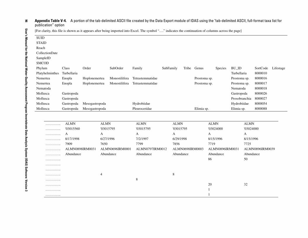
g the "tab-delimited ASCII, full-format taxa list for

columns across the page]

Species BU_ID SortCode Lifestage

Turbellaria 8000010

a sp. Prostoma sp. 8000016

a sp. Prostoma sp. 8000017

Nematoda 8000018

Gastropoda 8000026

Prosobranchia 8000027

Hydrobiidae 8000054

sp. Elimia sp. 8000088

ALMN ALMN

'03024000 '03024000

A A

8/15/1996 8/15/1996

7719 7725

ALMN0896IRM0031 ALMN0896IRM0039

Abundance Abundance

86 50

20 32

1

1

96

User’s M


ater-Quality A

ssessment Program

Invertebrate Data A

nalysis System (ID

AS) Softw

are: Version 3

Appendix Table V-4. A portion of the tab-delimited ASCII file created by the Data Export module of IDAS usinpublication” option [For clarity, this file is shown as it appears after being imported into Excel. The symbol “….” indicates the continuation of

SUID

STAID

Reach

CollectionDate

SampleID

SMCOD

Phylum Class Order SubOrder Family SubFamily Tribe Genus

Platyhelminthes Turbellaria

Nemertea Enopla Hoplonemertea Monostilifera Tetrastemmatidae Prostom

Nemertea Enopla Hoplonemertea Monostilifera Tetrastemmatidae Prostom

Nematoda

Mollusca Gastropoda

Mollusca Gastropoda

Mollusca Gastropoda Mesogastropoda Hydrobiidae

Mollusca Gastropoda Mesogastropoda Pleuroceridae Elimia

…………. ALMN ALMN ALMN ALMN

…………. '03015560 '03015795 '03015795 '03015795

…………. A A A A

…………. 8/17/1998 6/27/1996 7/2/1997 6/29/1998

…………. 7909 7650 7799 7856

…………. ALMN0898IRM0031 ALMN0696IRM0001 ALMN0797IRM0012 ALMN0698IRM0003

…………. Abundance Abundance Abundance Abundance

………….

………….

………….

…………. 4 8

…………. 8

………….

………….

………….

s selected in the Data Export module (for example, CANOCO, Cornell Ecology Package, MVSP, s also uses the *.cnd extension (for example, aaaa_key.cnd).

TX10 TX20

TX330

S10 S20

S60

Appendixes

97

Appendix Table V-5. Selected lines from the ASCII file created when the CANOCO-condensed format option i[This format provides an efficient means of getting data into many statistical packages that calculate community ordinationsPC_ORD). The file extension for CANOCO-condensed format file is *.cnd. The “key” file that documents the abbreviationThe symbol “:” indicates where lines of data have been omitted]

ALMN Invert data. RTH, no ambig taxa(I3,5(I4,F10.3)) 5 1 9 58.000 21 19.000 22 134.000 23 38.000 28 19.000 1 29 1076.000 31 8.000 43 749.000 44 1.000 55 19.000 1 72 230.000 82 65.747 90 21.538 95 12.574 97 1207.141 1 98 23.000 114 148.858 116 24.594 125 24.594 127 28.477

:: 1 305 19.355 310 134.000 324 77.000 326 19.000 332 2.000 1 335 76.000 2 3 4.000 23 33.000 29 79.000 30 2.000 43 36.277 2 56 43.308 59 1.312 62 11.811 69 178.668 75 58.171 2 79 66.481 82 108.489 95 2.358 98 16.123 106 1.000

:: 67 288 22.627 291 158.389 292 316.778 294 34.479 303 11.852 67 305 22.627 306 11.852 319 32.000 331 12.000 335 525.000

0 TX1 TX2 TX3 TX4 TX5 TX6 TX7 TX8 TX9 TX11 TX12 TX13 TX14 TX15 TX16 TX17 TX18 TX19 :: TX321 TX322 TX323 TX324 TX325 TX326 TX327 TX328 TX329 TX331 TX332 TX333 TX334 TX335 TX336 TX337 TX338 TX339 S1 S2 S3 S4 S5 S6 S7 S8 S9 S11 S12 S13 S14 S15 S16 S17 S18 S19 :: S51 S52 S53 S54 S55 S56 S57 S58 S59 S61 S62 S63 S64 S65 S66 S67

APPENDIX VI: ERROR MESSAGES

The following is an alphabetical list of error messages that can be generated by the IDAS program. Typically, error messages are displayed in an error message window with a descriptive title at the top and information on the type of error in the body of the window. An “OK” button allows the user to exit the error message window. In the following list, the error window title is given in all-capital letters followed by the body of the error message. An explanation of the error and corrective actions to take are given in italics.

DATA ENTRY ERROR. Number of sites must be an integer greater than zero. Attempted to enter a number less than one (e.g., 0.1) or a non-numeric value when entering criteria for eliminating rare taxa based on number of sites in the Data Preparation module.

DATA ENTRY ERROR. Value must be numeric. Attempted to enter a non-numeric value in a data entry form that requires numeric data.

DATA ENTRY ERROR. Percent of sample abundance must be between 0 and 100. Attempted to enter a number less than 0 or greater than 100 when specifying the criteria for eliminating rare taxa based on the percentage of abundance contributed by the taxon in the Data Preparation module.

EMPTY DATA TABLE. No records encountered in data table [data table name] in file [Access file name]. Consequently, IDAS cannot display data for this data table. The IDAS function ‘View’ tried to display data for an Access data table that did not contain any data. Click on ‘OK’, exit IDAS, and examine the data table to determine why it contains no data.

EMPTY SPREADSHEET. No records encountered in spreadsheet [spreadsheet name] in file [file name]. Consequently, IDAS cannot display data for this spreadsheet. The IDAS function ‘View’ tried to display data for an Excel spreadsheet that did not contain any data. Click on ‘OK’, exit IDAS, and examine the spreadsheet to determine why it contained no data.

ERROR: ATTRIBUTE FILE IS MISSING. IDAS was unable to find the attribute file ('Attributes.xls') at the default location [default location]. This file is required for the calculation of tolerance and functional group metrics. Do you want to manually search for the attributes file? This error occurs when the invertebrate attributes file is not located in the directory that IDAS identified as the default directory when it started. Normally, this should be the directory where IDAS.EXE is stored. Click on ‘Yes’ to browse the hard drive and locate the attributes file. Clicking on ‘No’ calls up an additional message box that allows you to proceed without the information contained in the attribute files (i.e., no tolerance or functional group metrics will be calculated) or exit the module.

ERROR ENCOUNTERED IN OPENING FILE. [error code] An error was encountered while opening a file in IDAS. This is a trappable, but unanticipated error. Copy the error code and report it to the author along with the files and circumstances under which this error occurred.

ERROR ENCOUNTERED IN SUBROUTINE [subroutine name]. [numeric error code and explanation provided by Visual Basic]. An unanticipated, but trappable error has occurred. Copy the information given in the error message, exit IDAS, and report the error message and circumstances that produced the error to the author.


ERROR IN DATA FILE. No sites (STAIDs) were encountered in the data set. Please close the data file or choose another file. The file that IDAS was attempting to read did not contain any station identifiers (column STAID). Click on ‘OK’, exit IDAS, and examine the file to determine why it did not contain any station identifiers.

ERROR IN DATA TABLE. The input data table [table name] does not contain data on abundance or density. Review the input data table and determine why it does not have a column of abundance or density data. The Access data table or Excel spreadsheet that IDAS was attempting to get data from contains no information on abundances. Click on ‘OK’ and exit IDAS. Examine the data file and determine if the columns ‘Abundance’ and ‘Density’ are present and, if so, whether there are data in these columns.

ERROR IN ENTRY OF OPTION FOR PROCESSING RARE TAXA. Percentages for processing rare taxa must be between 0 and 100. The ‘delete rare taxa based on percentage abundance’ option requires that the criteria values be entered as percentages (0-100%). This error occurs when a value less than 0 or greater than 100 is entered. Click on ‘OK’ and enter a value between 0 and 100.

ERROR IN FILE TYPE. File [input file name] is not an Excel or Access file. Select another file. The user attempted to open a file that was not an Excel workbook (*.xls) or an Access database (*.mdb). Click on ‘OK’ and select another file for processing.

ERROR IN % ABUNDANCES. The total proportion of abundance/density accounted for by the selected taxa – [value] – is outside the range of acceptable values (99.9-100.1). Correct one or more of the % abundance/density values assigned to the selected taxa. This error occurs in the Data Preparation module when the user is selecting children to associate with ambiguous parents for samples without children. The user selects the children to associate with the parents and IDAS automatically calculates the relative abundance of the selected children based on their abundance in all samples combined. The user can override this selection and enter their own percentages. This error occurs when the percentages assigned by the user do not add up to 100 ± 0.1 %. Click on ‘OK’ and correct the percentages.

ERROR IN SAMPLE LIST. No samples encountered in the table ‘tblSorted’. Check the data files to ensure that you are using the correct file. Processing the file resulted in a new data set that is blank. Click on ‘OK’ and select a new set of processing parameters and(or) a new data file for processing.

ERROR IN SAMPLE LIST. No taxa encountered in the sample [SMCOD] in ‘tblSorted.’ Check the data fields to ensure that you are using the correct file. Processing the file resulted in a new data set that contains no taxonomic information. Click on ‘OK’ and select a new set of processing parameters and(or) a new data file for processing.

ERROR IN TAXA LEVEL OPTIONS. The upper taxa limit chosen for resolving ambiguities [upper taxa level] is lower than the limit chosen as the lowest taxonomic level [lowest taxa level]. Either change the selection for lowest taxonomic level or change the upper taxonomic limit for aggregation. The upper taxa limit chosen for resolving ambiguities using method 2 (Delete children of ambiguous parents and add their abundance to the parents) is lower than the limit specifying the lowest taxonomic level (e.g., genus, family). The upper taxa limit must be a higher taxa level than the lowest taxonomic level or no data will be extracted. Click on ‘OK’ and change one or both of these criteria levels before proceeding in the Data Preparation module.

Appendixes 99

ERROR IN TAXA LIST. The data file contained no taxa. Choose another file. Processing the data table/spreadsheet file resulted in a new data set that contains no taxonomic information. Click on ‘OK’ and select a new data file for processing.

INCOMPATIBLE TABLE FORMATS. The columns in table/spreadsheet [data table or spreadsheet name] are inconsistent with columns in other tables/spreadsheets. These tables cannot be combined. Please choose a different set of tables to combine. IDAS has detected that a table or spreadsheet that you are trying to combine with other tables/spreadsheets in the Edit Data module has a different format (different number of columns and(or) different column names). IDAS will combine only tables/spreadsheets that have similar formats. Exit the module and examine the tables/spreadsheets to determine where they differ and how to make them compatible.

MISSING DATA! No abundance or density data encountered in [table or spreadsheet][table or spreadsheet name] of file [file name]. Check this file and table to be sure it contains the proper data. The program will stop processing data and return to the opening screen of the Edit Data module. The selected data table or spreadsheet contained no abundance or density data. Exit IDAS and examine the data table/spreadsheet to determine if the abundance or density columns are incorrectly labeled, missing, or empty. Correct the problem before trying to process these data further.

MISSING DATA! No samples were encountered in [table or spreadsheet] [table or spreadsheet name] of file [file name]. Check this file and table to be sure it contains the proper data. The program will stop processing data and return to the opening screen of the Edit Data module. The selected data table or spreadsheet contained no samples (i.e., SAMPLEID column is blank). Exit IDAS and examine the data table/spreadsheet to determine why the SAMPLEID column is blank and correct this problem before trying to process this data set further.

MISSING DATA! No sites were encountered in [table or spreadsheet] [data table or spreadsheet name] of file [file name]. Check this file and table to be sure it contains the proper data. The program will stop processing data and return to the opening screen of the Edit Data module. The selected data table or spreadsheet contained no sites (i.e., STAID column is blank). Exit IDAS and examine the data table/spreadsheet to determine why the STAID column is blank and correct this problem before trying to process this data set further.

MISSING RECORDS. There are no records in the data file. Execution of the Data Export module will be

terminated. Please check the data contained in file [input file name] before further processing. The data table/spreadsheet that was read by the Data Export module contains no records. Click on ‘OK’ and exit IDAS. Examine the data table/spreadsheet to determine why it contains no records.

MISSING SAMPLEID’S. There are no samples (SAMPLEID’s) in the data file. Execution of the Data Export module will be terminated. Please check the data contained in file [input file name] before further processing. The data table/spreadsheet that was read by the Data Export module contains no samples (SAMPLEID’s). Click on ‘OK’ and exit IDAS. Examine the data table/spreadsheet to determine why it contains no samples.

MISSING SORT CODE. The sort code is missing for [taxa name] in the 'Accept Selection(s)' routine of frmSelectChild. IDAS was unable to find a sort code in the data set that corresponds to the name of a child that was associated with an ambiguous parent. Exit IDAS and check the data file to make sure that there are not any missing sort codes.


MISSING TAXA. There are no taxa (BU_ID’s) in the data file. Execution of the Data Export module will be terminated. Please check the data contained in file [input file name] before further processing. The data table/spreadsheet that was read by the Data Export module contains no taxa names (BU_ID’s). Click on ‘OK’ and exit IDAS. Examine the data table/spreadsheet to determine why it contains no taxa names.

NO INDEX CHOSEN. No diversity or similarity indices were chosen. Please select one or more indices to calculate. The user tried to calculate diversity and similarity indices in the Calculate Diversities and Similarities module without first selecting the indices to calculate. Click on ‘OK’ and select one or more indices.

NO QMH SMCODS WERE ENCOUNTERED. IDAS will reset the ‘Data Preparation’ module. The Data Preparation module was attempting to form QUAL samples (QMH + RTH and(or) DTH), but no QMH samples were encountered. Click on ‘OK’ and exit IDAS. Examine the data table/spreadsheet and determine why there were no QMH samples in the data set.

NO RECORDS FOUND IN DATA SET! No records encountered in the data set. IDAS will quit processing data and will return to the opening window of the ‘Data Export’ module. The data table/spreadsheet that was read by the Data Export module contains no records. Click on ‘OK’ and exit IDAS. Examine the data table/spreadsheet to determine why it contains no records.

NO RECORDS IN DATABASE. No records were found in table [table of similarity values]. IDAS will exit the ‘SaveSimToAccess’ subroutine and return to the opening screen of the ‘Calculate Diversities and Similarities’ module. The subroutine that calculates similarity indices produced no similarity values so there are no similarity values to save to the Access database. Exit IDAS and examine the data table to determine why IDAS could not calculate similarities for this data set.

NO RECORDS IN FILE! There are no records for invertebrate sample areas in the table [table or spreadsheet name] in the file [input file name]. Select another file or table. The Data Preparation module could not find sample areas (AreaSampTot) in the file that the user designated as the source for sample areas. Click on ‘OK’ and select another data table/spreadsheet that holds sample areas or exit IDAS and examine the sample area file to determine why there were no sample areas detected.

NO RECORDS IN FILE! There are no records in the abundance file. Select another file. The data file that was read by IDAS contained the correct column headers, but no data. Click on ‘OK’ and select another data table/spreadsheet for processing or exit IDAS and examine the data table/spreadsheet to determine why it contains no data.

NO RECORDS SELECTED! No records match the criteria specified for subsetting these data. Please choose another set of criteria or click on 'File' and 'Close' to process another data set or 'Exit' to leave the Edit Data module. The combination of criteria specified for subsetting data tables/spreadsheets in the Edit Data module has resulted in an empty data set. IDAS will not generate empty data tables/spreadsheets. Click on ‘OK’ to return to the criteria window and specify a new set of criteria.

Appendixes 101

NO [RTH, QMH, DTH] SAMPLES IN DATA SET. The user has requested an analysis that requires [RTH, DTH, or QMH] samples. No [RTH, DTH, or QMH] samples were detected in the file [input file name]. IDAS will cease processing these data and will return the user to the opening screen of the ‘Data Preparation’ module. The user requested a data processing procedure in the Data Preparation module that requires RTH, DTH, and(or) QMH samples, but no RTH, DTH, and(or) QMH samples were found in the data set. For example, the QUAL option could have been invoked on a file that had been processed through the Edit Data module so it only contained quantitative samples (RTH and DTH). Therefore, IDAS would not have been able to find any QMH samples to pair with RTH and DTH samples, which would have generated this error. Click on ‘OK’ and select only the sample types that exist in the data file.

NO SAMPLES ENCOUNTERED. No RTH, DTH, or QMH samples encountered in file [input file name]. IDAS will cease processing data and return to the opening screen of the Data Preparation module. Even though the data structure was correct, IDAS could not find RTH, DTH, or QMH samples in the data set. Click on ‘OK’ and select a new data table/spreadsheet to process or exit IDAS and examine the data file to determine why it does not contain RTH, DTH, or QMH samples.

REQUIRED SPREADSHEET(S) ARE MISSING. The file [file name] did not contain the required spreadsheet [ATTRIB and(or) EQTX]. IDAS cannot calculate tolerance or functional group metrics. Metric calculations will be terminated and the user will be returned to the opening screen of the 'Calculate Metrics' module. This error occurs when the invertebrate attributes file selected by the user (default name: Attributes.xls) does not contain spreadsheets named ATTRIB (attributes) and(or) EQTX (list of equivalent taxa). Typically, this error occurs when the attributes file is not in the default location and the user selects the wrong file while browsing the hard disk. Click on ‘OK’ and exit IDAS. Locate a copy of the attributes file, and copy it into the default location (that is, the same location from which IDAS.EXE is launched).

SELECT ITEM FROM LIST. No worksheet or table name has been selected! Please select an item by clicking on its name in the text box and then clicking on the 'Select' button or click on 'Cancel' to cancel this operation. The user did not specify a data table or worksheet to open. This usually occurs when the user clicks on ‘Select’ without first clicking on the desired data table/spreadsheet name listed in the text box. Click on ‘OK’ and then select the desired data table/spreadsheet, or click on ‘Cancel’ to exit this function.

SELECT PROCESSING OPTION! No method was selected for resolving ambiguities. Please select a method (1 – 5) from the list. IDAS cannot proceed unless the user specifies how to process ambiguous taxa. Click on ‘OK’, click on one of the radio buttons associated with ambiguous taxa resolution methods 1 to 5, and then click on ‘Run’ to process data in the Data Preparation module.

TABLE NAME SELECTION. Table name already exists in the database. Please enter another name. Table/spreadsheet names used to store output must not already exist in the Excel workbook or Access database. Click on ‘OK’ and enter a name that is not listed in the text box that shows the contents of the workbook or database.

TABLE NAME SELECTION. Table name contains one or more illegal characters. Please enter a new table name.

Table/spreadsheet names can only include letters, numbers, and the underline symbol. Click on ‘OK’ and enter a name that is 15 characters or less in length, starts with a letter, and contains only letters, numbers, and the underline symbol.


TABLE NAME SELECTION. Table name does not begin with a letter. Please enter a new table name. The table name entered by the user must begin with a letter. Click on ‘OK’ and enter a table name that is 15 characters or less in length, starts with a letter, and includes only letters, numbers, and the underline symbol.

TABLE NAME SELECTION. Table name is blank. Please enter a new table name. The user clicked on ‘Select’ before entering a new table/spreadsheet name. Click on ‘OK’ and enter a table name before clicking on ‘Select.’ Names of tables/spreadsheets used to store output must be 15 characters or less in length, start with a letter, and contain only letters, numbers, and the underline symbol.

TABLE NAME SELECTION. Table name is too long (>15 characters). Please enter a new table name. Names of tables/spreadsheets used to store output must be 15 characters or less in length, start with a letter, and contain only letters, numbers, and the underline symbol. Click on ‘OK’ and enter a new table or spreadsheet name.

TABLE/SPREADSHEET FORMAT FOR COMBINING DATA NOT RECOGNIZED! File [file name] did not contain any tables or spreadsheets with a format that is compatible with this IDAS module. Please check the format of this table/spreadsheet and modify it to conform to the requirements of this module. IDAS will stop processing data and return to the opening screen of this module. The data table or spreadsheet did not contain a format that was consistent with those recognized by IDAS (that is, Bio-TDB format and ‘processed’ format). Exit IDAS and check the format of the data table or spreadsheet in question.

TABLE/SPREADSHEET FORMAT NOT RECOGNIZED! File [input file name] did not contain any tables or spreadsheets with a format that is compatible with this IDAS module. Please check the format of the table/spreadsheet and modify it to conform to the requirements of this module. IDAS will stop processing data and return to the opening screen of this module. IDAS could not find any data tables or spreadsheets with the appropriate format for this module. Click on ‘OK’ and select another file to process or exit IDAS and examine the data file to determine why it does not match the Bio-TDB (appendix table I-1) or processed (appendix table II-1) data formats.

Appendixes 103

userâ€™s manual for the nati onal water-quality assessment program

Documents