user’s guide to the weighted-multiple-linear …. department of the interior u.s. geological...

U.S. Department of the InteriorU.S. Geological Survey

Techniques and Methods 4–A8

User’s Guide to the Weighted-Multiple-Linear Regression Program (WREG version 1.0)


By Ken Eng, Yin-Yu Chen, and Julie E. Kiang

Techniques and Methods 4–A8

U.S. Department of the InteriorU.S. Geological Survey

U.S. Department of the InteriorKEN SALAZAR, Secretary

U.S. Geological SurveyMarcia K. McNutt, Director

U.S. Geological Survey, Reston, Virginia: 2009

For more information on the USGS—the Federal source for science about the Earth, its natural and living resources, natural hazards, and the environment, visit http://www.usgs.gov or call 1–888–ASK–USGS.

For an overview of USGS information products, including maps, imagery, and publications, visit http://www.usgs.gov/pubprod.

To order this and other USGS information products, visit http://store.usgs.gov.

Any use of trade, product, or firm names is for descriptive purposes only and does not imply endorsement by the U.S. Government.

Although this report is in the public domain, permission must be secured from the individual copyright owners to reproduce any copyrighted materials contained within this report.

Suggested citation:Eng, Ken, Chen, Yin-Yu, and Kiang, J.E., 2009, User’s guide to the weighted-multiple-linear-regression program (WREG version 1.0): U.S. Geological Survey Techniques and Methods, book 4, chap. A8, 21 p. (Also available at http://pubs.usgs.gov/tm/tm4a8.)

On the cover: Examples of plots resulting from analysis of data with the weighted-multiple-linear regression (WREG) program (version 1.0).

http://pubs.usgs.gov/tm/tm4a8/

iii

Contents

Introduction.....................................................................................................................................................1Multiple-Linear Regression ..........................................................................................................................2Independent and Dependent-Variable Transformations .........................................................................2Estimation of Multiple-Linear-Regression Parameters ...........................................................................2

Ordinary Least Squares (OLS) ............................................................................................................3Weighted Least Squares (WLS) .........................................................................................................3Generalized Least Squares (GLS) ......................................................................................................4

Performance Metrics ....................................................................................................................................5Model- and Time-Sampling Errors .....................................................................................................5Coefficient of Determination, R2, R2

adj, and R2pseudo .................................................................................................................................6

Leverage and Influence Statistics .....................................................................................................6Significance of Regression Parameters ...........................................................................................7

Definition of Regions .....................................................................................................................................7Use of the WREG Program ...........................................................................................................................8Program Requirements .................................................................................................................................8Installation.......................................................................................................................................................8Input Files ........................................................................................................................................................8

SiteInfo.txt ..............................................................................................................................................9FlowChar.txt .........................................................................................................................................10LP3G.txt .................................................................................................................................................10LP3K.txt .................................................................................................................................................11LP3s.txt..................................................................................................................................................12UserWLS.txt .........................................................................................................................................12USGS########.txt................................................................................................................................13

Running the Program...................................................................................................................................13Set Up Model ................................................................................................................................................13

Select Variables ..................................................................................................................................13Select Transformations ......................................................................................................................13Model Selection ..................................................................................................................................15

GUI Outputs ...................................................................................................................................................16Regression Summary .........................................................................................................................16Residuals Versus Estimated Flow Characteristics ........................................................................17Leverage Values Versus Observations ............................................................................................17Influence Values Versus Observations ...........................................................................................17

Output Files ...................................................................................................................................................17ConventionalOLS.txt, ConventionalWLS.txt, and ConventionalGLS.txt ......................................18RegionofInfluenceOLS.txt, RegionofInfluenceWLS.txt, and RegionofInfluenceGLS.txt .........19RegressionModel.txt ..........................................................................................................................20InvXLX.txt..............................................................................................................................................20SSres.txt and SStot.txt .......................................................................................................................20EventLog.txt..........................................................................................................................................20

iv

Other Program Notes ..................................................................................................................................20Acknowledgments .......................................................................................................................................20References Cited..........................................................................................................................................20

Figures 1. Examples of input file SiteInfo.txt in text tab-delimited format .....................................................9 2. Example of input file FlowChar.txt in text tab-delimited format ...................................................11 3. Example of input file LP3G.txt ............................................................................................................11 4. Example of input file LP3K.txt ............................................................................................................11 5. Example of input file LP3s.txt ............................................................................................................12 6. Example of input file UserWLS.txt ....................................................................................................12 7. An example of a USGS########.txt file for streamflow-gaging station 09183000 ....................13 8. Example of WREG window used to select variables to be used in the regression .................13 9. Examples of WREG window for selecting transformations .........................................................14 10. Example of WREG window for selecting the regression ..............................................................15 11. Example of WREG window for selecting parameters of the smoothing function for

correlation as a function of distance between streamflow-gaging stations ...........................15 12. Example of WREG window for selecting option to include uncertainty in skew .....................16 13. WREG window showing the regression results for an OLS regression using the

parameters and transformations specified in figure 9 .................................................................16 14. Examples of plots ................................................................................................................................16 15. Example of output file ConventionalOLS.txt ....................................................................................17 16. Example of output file ConventionalWLS.txt ..................................................................................18 17. Example of output file ConventionalGLS.txt ....................................................................................18 18. Example of output file RegionofInfluenceOLS.txt ..........................................................................19 19. Example of regression model equation shown by RegressionModel.txt ..................................20 20. Example of InvXLX.txt output file ......................................................................................................20 21. Examples of SSres.txt and SStot output files .................................................................................20

Tables 1. WREG input files ...........................................................................................................................8 2. WREG output files .......................................................................................................................17

v

Conversion Factors

Multiply By To obtainLength

inch (in.) 2.54 centimeter (cm)inch (in.) 25.4 millimeter (mm)foot (ft) 0.3048 meter (m)mile (mi) 1.609 kilometer (km)mile, nautical (nmi) 1.852 kilometer (km)yard (yd) 0.9144 meter (m)


By Ken Eng, Yin-Yu Chen,1 and Julie E. Kiang

1Former U.S. Geological Survey volunteer.

IntroductionStreamflow is not measured at every location in a stream

network. Yet hydrologists, State and local agencies, and the general public still seek to know streamflow characteristics, such as mean annual flow or flood flows with different exceed-ance probabilities, at ungaged basins. The goals of this guide are to introduce and familiarize the user with the weighted-multiple-linear regression (WREG) program, and to also provide the theoretical background for program features. The program is intended to be used to develop a regional estima-tion equation for streamflow characteristics that can be applied at an ungaged basin, or to improve the corresponding estimate at continuous-record streamflow gages (henceforth referred to as simply gages) with short records. The regional estimation equation results from a multiple-linear regression that relates the observable basin characteristics, such as drainage area, to streamflow characteristics (for example, Thomas and Benson, 1970; Giese and Mason, 1993; Ries and Friesz, 2000; Eng and others, 2005; Eng and others, 2007a; Eng and others, 2007b; Kenney and others, 2007; Funkhouser and others, 2008).

The general multiple-linear regression for estimating a streamflow characteristic can be given by

, (1)

where y is the streamflow characteristic (dependent variable),

xik are basin characteristics (independent variables),

i (=1, 2, 3,…, n) is the index for gage i, k is the number of basin characteristics, β0, β1, β2, and βk are the regression parameters, and δi is the model error.

A critical issue in regional analyses is to understand the various sources of variability and error in the data. By understanding these sources, a user can select the appropriate approaches to estimate the regression parameters in equation 1, and the appropriate network of gages forming the region used to develop an estimate. Three approaches to estimate

regression parameters are provided in the WREG program: ordinary-least-squares (OLS), weighted-least-squares (WLS), and generalized-least-squares (GLS). All three approaches are based on the minimization of the sum of squares of differ-ences between the gage values and the line or surface defined by the regression. The OLS approach is appropriate for many problems if the δi values are all independent of one another, and they have the same variance. Streamflow characteristics are estimated at gages using the available length of streamflow record. Because the length of record varies among gages, the precision of these estimates also varies, meaning that different δi values will have different variances.

A way to address the variation in the precision of estimated streamflow characteristics at each gage is to weight gages differ-ently using WLS or GLS. A WLS approach reflects the preci-sion of the estimated streamflow characteristic at that gage. An additional issue is that concurrent flows observed at different gages in a region exhibit cross correlations. If these correlations are not represented in a regional analysis, the regression param-eters are less precise, and estimators of precision are inaccurate. A regional analysis that accounts for the precision of estimated streamflow characteristics, and the cross correlations among these characteristics, is known as GLS.

In addition to the variation and error in the data, the regression parameters in equation 1 are impacted by the choice of a network of gages forming a region. In a “conventional” regression, a region can be defined in several ways before a multiple-linear-regression study is initiated, such as by political boundaries or by physiographic boundaries. Within the con-text of “conventional” regressions, regions can also be defined during the regression study by using geographic information as an independent variable in the regression. Such regions can be defined using a variety of criteria, such as geographic grouping of similar residuals from an overall regression (Wandle, 1977), use of watershed boundaries (Neely, 1986), or physiographic characteristics. When performing a conventional analysis, a user of WREG must define the regions before using the program. WREG allows the user to perform conventional regressions using either OLS, WLS, or GLS.

An alternative to the conventional approach of pre-defining regions using political or physiographic boundaries is to define a region for each location of interest. This “region-of-influence” (RoI) regression approach defines a region and associated

2 User’s Guide to the Weighted-Multiple-Linear Regression Program (WREG, v. 1.0)

multiple-linear regression for every ungaged basin (for example, Acreman and Wiltshire, 1987; Burns, 1990; Tasker and oth-ers, 1996; Merz and Blöschl, 2005; Eng and others, 2005; Eng and others, 2007a; Eng and others, 2007b). A regression is formed on a subset of gages for which the values of independent variables are, by some measure, closest to those at the ungaged basin of interest. While the WREG program allows testing of RoI regressions, the application of RoI regression to ungaged basins must be accomplished using other programs, such as the National Streamflow Statistics (NSS) Program (Ries, 2006).

The first part of this report provides an overview of the multiple-linear regression techniques that are employed by WREG. It is followed by a step-by-step guide to the actual use of the program, including a description of the input files, the use of the graphical user interface, and an explanation of the output files.

Multiple-Linear RegressionIn practice, the dependent variable, yi, in equation 1 is an

estimate, , often obtained from a limited sample size at each gage. The associated time-sampling error for the ith gage, ηi, is defined by

. (2)

Substituting equation 2 into equation 1 gives

, (3)

where εi = δi+ ηi (δi as given by equation 1). The ηi values from gages close together will generally be

correlated, because the finite sample of observed streamflows at one gage temporally overlaps the sample from another and temporal variations of streamflows are spatially correlated. Thus, the cross correlation between ηi and ηj for gage i and j will depend upon the cross correlation of concurrent flows at the two gages, and the number of concurrent years of record included in the dataset.

For a collection of gages with associated dependent and independent variables, equation 3 can be conveniently written in matrix notation as

, (4)

where

, (5)

and the total error, ε, is a random variable with a mean equal to zero and variance equal to σε

2.

Independent and Dependent-Variable Transformations

The independent and dependent variables used in equation 5 can be transformed to obtain a linear relation-ship between the and X values. Common transformations include log (base 10), log (natural), and addition or subtrac-tion of a constant. A user of WREG must choose appropriate transformations in the graphical user interface (GUI) before a multiple-linear regression is performed. A general transforma-tion equation used by WREG is given as

, (6)

where V is the dependent or independent variable to be transformed,

Vnew is the transformed independent or dependent variable,

f is either the log (base 10), log (natural), or exponential function, or a transformation can be omitted.

C1, C2, C3, and C4 are constants entered by the user.Use of equation 6 for transforming variables is further dis-

cussed in the section of this report titled Select Transformations.

Estimation of Multiple-Linear-Regression Parameters

Following transformations of the dependent and indepen-dent variables, the transformed variables are used in WREG to estimate multiple-linear-regression parameters. When using any of the least squares regression approaches (OLS, WLS, or GLS), the regression parameters are estimated by

. (7)

where XT is the transpose of matrix X, Λ-1 is the inverse of the weighting matrix Λ (I = Λ-1Λ,

where I is equal to the identity matrix).The Λ matrix is constructed differently for OLS, WLS,

and GLS, as described in the following sections. Once is determined, it can be used to estimate the regression estimate of at the ith gage, iR, as

. (8)

However, a user should first check if the regression is adequate.

The estimators of Λ used in WREG for WLS and GLS approaches are applicable only to frequency-based streamflow characteristics. Alternative estimators of Λ to those presented in this manual can be explored using a user-defined option in

Estimation of Multiple-Linear-Regression Parameters 3

WREG (see section UserWLS.txt) for non-frequency-based streamflow characteristics, such as flow-duration exceedences.

Ordinary Least Squares (OLS)For the OLS approach, β is estimated by (for example,

Montgomery and others, 2001)

, (9)

where . (10)

The OLS approach is suitable for estimating regres-sion parameters when there is no variation in the precision of calculated dependent variables among gages, and the errors in equation 5 are independent of each other.

Weighted Least Squares (WLS)For the WLS approach, β is estimated by (for example,

Tasker, 1980)

, (11)

where ΛWLS is the covariance matrix used to determine weights.

The components of the ΛWLS matrix are a function of the type and source of the dependent variable. As with the OLS approach, the WLS approach is suitable when the errors in equation 5 are independent. However, for the WLS approach, weights in the weighting matrix are assigned so that gages that have more “reliable” estimates of streamflow characteristics have larger weights.

For streamflow characteristics calculated from a log-Pearson Type III frequency analysis (Bulletin 17B of the Inter-agency Advisory Committee on Water Data, 1982), Tasker (1980) provides a method for estimation of ΛWLS that is used by WREG for this option:

, (12)

where

, and (13)

, (14)

where is the model-error variance, mi is the record length for the ith gage,

is the observed mean-square error (MSE)of estimate using ordinary-least-squares approach,

is the arithmetic average of the log-Pearson Type III deviates for all gages in the regression, and

is the arithmetic average of the skew values at all gages (either at-gage skew, g, or weighted skew, Gw; explained below).

The log-Pearson Type III deviate values are a function of probability of exceedence and g (Interagency Advisory Com-mittee on Water Data, 1982). is the arithmetic average of standard deviation of the annual-time series of the streamflow characteristic estimated by regression. This “sigma regression” is determined by OLS regression of the standard deviation of the annual-time series at each gage against basin characteris-tics at each gage (Tasker and Stedinger, 1989),

, (15)

where σi is the standard deviation of the annual-time series of the streamflow characteristic for the ith gage,

xik is the kth basin characteristic for the ith gage,

α0, βσ1, βσ2, and βσk are parameters, and εσ is the model error for the sigma regression.

The σi values are a required input into the WREG pro-gram as discussed in section LP3s.txt.

The weighted skew for the ith gage is given by (Bulletin 17B of the Interagency Advisory Committee on Water Data, 1982)

, (16)

where GR,i is the regional skew estimate applicable to the ith gage, and

, (17)

where is equal to the estimated mean square error of the skew value at the gage, and

is the estimated mean square error of the regional skew values.

A variety of methods are available to determine GR values (Bulletin 17B of the Interagency Advisory Committee on Water Data,1982). Either g or Gw values are required input to WREG program as discussed in section LP3G.txt.

An alternative approach to calculating is presented by Stedinger and Tasker (1986). Their estimator is demonstrated to be more precise than equation 13, but their study did not include a mix of approaches to compute streamflow character-istics at partial-record-stream gages (Funkhouser and others, 2008). Use of equations 12 to 14 within the WREG program allows future versions to account for this mix of approaches for partial-record-stream gages.


Generalized Least Squares (GLS)For streamflow characteristics calculated from a log-Pearson Type III frequency analysis, a GLS

approach described by Stedinger and Tasker (1985) builds on the WLS approach by accounting for both correlated streamflows and time-sampling errors. This GLS approach estimates the β values by

, (18)

where ΛGLS is a matrix containing the estimates of the covariances of εi among gages.The main diagonal elements of ΛGLS thus include a part associated with the model error, δi, and

all elements include the effect of the time-sampling error, ηi. In Tasker and Stedinger (1989), ΛGLS is estimated by

, (19)

where i and j are indices of locations of gages in the region of interest, Gi and Gj are skew values equal to either g or Gw (equation 16) values for gages i and j, mi and mj are record lengths for gages i and j, mij is the concurrent record length for gages i and j, and ρij is an estimated value for the cross-correlation of the time series of flow values used to

calculate the streamflow characteristic at gages i and j.Values of the cross-correlation are estimated approximately by (Tasker and Stedinger, 1989)

, (20)

where dij is the distance between gages iand j in miles, and θ and α are dimensionless parameters estimated from data as discussed in section Model

Selection.The values in equation 19 and the values in equation 18 are jointly determined by iteratively

searching for a nonnegative solution to (Stedinger and Tasker, 1985)

. (21)

Equation 19 does not account for error associated with estimating G. Depending on the actual magnitude of errors in estimation of skew, this additional error may unduly influence the estimation of β. Griffis and Stedinger (2007) proposed an approach to account for the uncertainty in the skew estimates in ΛGLS, and this approach is used as an option by WREG. As implemented in WREG, this option assumes that weighted skews are provided by the user, and so this option should be activated only when weighted skews were used. The modified ΛGLS matrix, ΛGLS,skew, is given by

, (22)

Performance Metrics 5

where and are the partial derivatives for gages i and j calculated from the Kite (1975; 1976) approximation for K given as

, (23)

where zp is the standard normal deviate corresponding to probability p.

The COV[gi,gj] in equation 22 is the covariance between the skew values at gages i and j, and is given by

, (24)

where is estimated by (Martins and Stedinger, 2002)

, and (25)

is equal to one if is positive and to minus one if is negative.

The Var(gi) and Var(gj) in equation 24 are approximated by (Griffis and Stedinger, 2009)

, (26)

where , (27)

, and (28)

. (29)

Equation 19 is a simplified version of equation 22 that assumes the skew is without error. Equation 19 is provided in the WREG program to reproduce previous studies that do not use equation 22.

Performance MetricsThe WREG program reports multiple performance

metrics for multiple-linear regressions, depending upon the options (OLS, WLS, or GLS) selected. Specific metrics are reported either in the GUI or the output files of WREG.

Model- and Time-Sampling ErrorsFor conventional OLS and RoI regressions, the residual

errors, ei, are computed as

, (30)

where is the estimated provided by the regression (see equation 8).

The residual mean square-error (MSE) is computed as

, (31)

where ei is calculated from equation 30.The MSE metric does not distinguish the proportion of

total error, εi that is composed of model error, δi, and time-sampling error, ηi. WLS and GLS regression provide estimates of the model error variance, , which is the same as the MSE only if the time sampling error variance, , is equal to zero.

For conventional regressions using WLS and GLS, WREG reports the average variance of prediction, AVP, as the perfor-mance metric (Tasker and Stedinger, 1986) and is given by

, (32)

where xp is a vector containing the values of the independent variables of the pth gage augmented by a value of one.

When corresponds to the logarithm of the variable of interest, equation 32 can be reported as a percentage of the pre-dicted value. When expressed in this way, the metric is known as the average standard error of prediction, Sp (Aitchison and Brown, 1957, modified for use of common logarithms), and is given by

. (33)

The standard model error as a percentage of the observed value can be calculated by substituting for AVP in equation 33. WREG program reports both Sp and the standard model error for WLS and GLS regressions.

For RoI regression, a regression is developed for each ungaged basin of interest. An overall performance metric reported by WREG program for RoI regressions using OLS, WLS, and GLS is a root mean square error, RMSE(%). This metric is similar to, but not the same as the prediction error sum of squares, PRESS, performance metric (for example, Montgomery and others, 2001). Every gage is treated in turn as an ungaged basin and a regression is developed for that site, and equations 30 and 31 are used to calculate a mean-square error value, MSERoI, that is used in place of AVP in equation 33 to give a root mean square error of prediction expressed as a percentage of the observed value, RMSE(%), given by (Eng and others, 2005; Eng and others, 2007a)

. (34)


Coefficient of Determination, R2, R2adj, and R2

pseudo

A metric reported by WREG for determining the propor-tion of the variation in the dependent variable explained by the independent variables in OLS regressions, is the coefficient of determination, R2, (Montgomery and others, 2001) given as

, (35)

where , and (36)

, (37)

where is the arithmetic mean of all values, SST is the total sum of squares that is equal to the sum

of the amount of variability in the observations, and

SSr is the residual sum of squares.SST and SSr values are provided as WREG output files

and can be used to calculate an adjusted coefficient of determi-nation, Radj

2, given as

. (38)

The adjusted Radj2 adjusts for the number of independent vari-

ables used in the regression.For WLS and GLS regressions, a more appropriate perfor-

mance metric than R2 or Radj2 is the R2pseudo described by Griffis

and Stedinger (2007). Unlike the R2 metric in equation 35 and Radj

2 in equation 38, R2pseudo is based on the variability in the dependent variable explained by the regression, after removing the effect of the time-sampling error. The R2pseudo is given as

, (39)

where is the model error variance from a WLS or GLS regression with k independent variables, and

is the model error variance from a WLS or GLS regression with no independent variables.

For RoI regressions using OLS, WLS, or GLS, no coef-ficient of determination values are reported in WREG.

Leverage and Influence StatisticsThe leverage metric is used to measure how far away

the value of one gage’s independent variables are from the centroid of values of the same variables at all other gages. This metric is reported for all gages in OLS, WLS, and GLS

regressions and RoI regressions. For non-RoI regressions, leverage, h, for the ith gage is given as

, (40)

where Λ is equal to either ΛOLS, ΛWLS, ΛGLS, or ΛGLS,skew.The leverage metric for RoI regressions using either

OLS, WLS, or GLS is given by (Eng and others, 2007b)

, (41)

where x0 is a vector of independent variables at a particular ungaged basin.

Unlike equation 40, equation 41 measures the leverage that each gage record in the RoI has on the ungaged basin 0. Leverage metrics associated with gages are considered large if these metrics exceed the criteria given by

, (42)

where Ch is a constant For conventional regression, Ch is equal to 2 in equa-

tion 42 and reflects the observation that values twice the average can be considered as unusually large. For RoI regression, Ch is equal to 4 (Eng and others, 2007b). A larger Ch value for RoI regression is recommended because h0

T values typically exhibit greater variability, and even negative values, whereas hii values are always positive. The hlimit is reported for regressions using OLS, WLS, and GLS in the output files of the WREG program, and is also shown visually on a plot of leverage values for each gage (see sections Output Files and Leverage Values Versus Observations).

The leverage metrics in equations 40 and 41 identify gages whose independent variables are unusual. Such unusual gages may or may not have any significant impact on the estimated regression parameters in equations 9, 11, and 18. An influence metric, such as Cook’s D (Cook, 1977), indicates whether a gage had a large influence on the estimated regres-sion parameter values. A generalized Cook’s D value for the ith gage is

, (43)

where v is the dimension of β, Λii is the ith main diagonal of the Λ covariance matrix,

and Lii is the ith main diagonal of X(XTΛ-1X)-1XT (Tasker

and Stedinger, 1989).

Definition of Regions 7

For regressions, a gage that has caused large influence is identified if Cook’s D exceeds the limit given by

. (44)

The Cook’s D limit calculated using equation 44 is reported in the WREG output files (see section Output Files), and visually on a plot of influence values (see section Influ-ence Values Versus Observation).

Significance of Regression ParametersRegression parameters are tested for significance by

WREG for regressions not using RoI regions. The null hypothesis is generally that the regression parameter is equal to zero, and the alternative hypothesis is that this parameter is not equal to zero. If the null hypothesis is not rejected at some predefined level of significance, such as 5%, then the associ-ated independent variable is removed from the regression. For regressions, the test statistic that is used to evaluate the null hypothesis is the Tvalue statistic given as

, (45)

where (Var βk) is the covariance value of βk, and is given as

. (46)

The Tvalue statistic in equation 45 is assumed to follow a Student’s t distribution, so probabilities or “p-values” can be calculated. If the critical level of significance is set to 5% (0.05), p-values associated with the calculated T value statistic from equation 45 that exceed 0.05 result in acceptance of the null hypothesis. In this case, the regression parameter is not considered significant. In WREG, coefficients that are not significant at the 5% significance level are flagged (see section Regression Summary).

Definition of RegionsThe region formed by a collection of gages can influence

the regression model and the significance of the results. For conventional regressions, the WREG program uses all gages that are input by the user to develop regressions using either OLS, WLS, or GLS. If a subset of gages from a larger data set is desired by the user, input files to WREG should be modified to reflect the smaller subset.

For RoI regressions, a select subset from all available gages is formed for every ungaged basin where an estimate

is desired. To use the RoI regression feature in WREG, a user would input all possible gages of interest, even though some gages might not be used in each RoI regression. Three approaches for defining hydrologic similarity among basins are available with WREG: independent or predictor-variable space RoI (PRoI) (for example, Burns, 1990), geographic space RoI (GRoI), and a combination of predictor-variable and geographic spaces called hybrid RoI (HRoI) developed by Eng and others (2007a).

For the GRoI option in WREG, a region of influence is formed using the n gages that are geographically the closest to the ungaged basin. In general, n is specified and is the same for every regression. The PRoI option in WREG is similar, but forms a region using the n closest gages in independent-variable space rather than geographic space. Thus, the region is com-prised of gages whose independent variables have values that are the most similar to the ungaged site. Distance in indepen-dent-variable space from the ungaged basin to the ith gage, Ri, is defined in a Euclidean sense as (for example, Burns, 1990)

, (47)

where , , and are the sample standard deviations of x1, x2, and xk, respectively (computed from data from the entire study region).

The HRoI approach uses a region of influence of the n closest gages in independent-variable space chosen from a sub-set of all gages having a geographic distance less than D from the ungaged basin. However, if fewer than n gages are available within the distance D of a given ungaged basin, then the limit D is ignored, HRoI reverts to GRoI and the n geographically closest gages are used. Thus, in the limit as D approaches zero, HRoI reduces to GRoI, and in the limit as D becomes arbitrarily large, HRoI reduces to PRoI (Eng and others, 2007a).

The user must determine the optimal D and n values. This determination can be accomplished by splitting the dataset into three equally sized subsets. Two of the three subsets are combined and used in an optimization step to calculate RMSE values for various values of n and D for HRoI regionalization. The same subsets are used to calculate RMSE values for vari-ous values of n for both PRoI and GRoI. The lowest result-ing values of RMSE and the corresponding values of n and D for HRoI and of just n for PRoI and GRoI are noted. The third subset is then used to evaluate model performance, by calculating the RMSE value associated with the optimal n and D determined in the previous step. All possible combinations of three subsets for this optimization-evaluation procedure are employed, and an overall RMSE value is then computed as the root mean-square value of the three individual subset values (Eng and others, 2005; Eng and others, 2007a).


Use of the WREG ProgramThe remainder of this report provides details on how to use

the Weighted-Multiple-Linear Regression Program (WREG). It can be used to set up, run, and evaluate a multiple-linear regres-sion. As described in previous sections, the methods used by the program have been customized for use in the regionalization of streamflow characteristics. Many of the default methods may not be suitable for other regression problems.

The program is driven by a graphical user interface that leads the user through the process of setting up a regression. A number of input files are required, and detailed output is avail-able in text files generated by WREG.

Notice.—MATLAB®. ©1984–2007 The MathWorks, Inc. was used to develop the graphical user interface and source code for WREG. The licensee’s rights to deployment of WREG are governed by the license agreement between licensee and MathWorks, and licensee may not modify or remove any license agreement file that is included with the MCR libraries. Installation of the application denotes accep-tance of the terms of the license specified in the file named license.txt in the folder WREGv1 included with this manual.

Program Requirements• Windows operating system.• Approximately 400 MB of free disk space.

Installation1. Unzip the distribution file (WREGv1.zip) and extract it

to the directory of your choosing. There should be four files—MCRInstaller.exe, WREGv1.exe, WREGv1.ctf, and license.txt—and two folders—WREG_Source_Code and Sample_Files.

2. Run the program MCRInstaller.exe. This program installs MATLAB Component Runtime, software that allows the WREG executable program to run. The installation

program leads you through the process with multiple GUI windows and may take several minutes to complete. Administrator privileges are required.

3. WREGv1.exe and WREGv1.ctf should be copied to another folder that contains input files and the program can be executed from that location. For example, copying the files into the folder Sample_Files will allow execu-tion of the program using the sample input files. Alterna-tively, input files can be copied to the directory in which WREGv1.exe and WREGv1.ctf were installed.

4. WREGv1.exe is the program executable file and it is now ready to run. WREGv1.ctf is a required file that must be located in the same working directory as WREGv1.exe. After WREG is run for the first time, another folder, WREGv1_mcr, will be created in the working directory. It contains additional files for running WREG. These files should not be changed. (If a new version of WREG is provided, the files WREGv1.exe and WREGv1.ctf and the folder WREGv1_mcr should all be deleted from the work-ing directory. The new WREG.exe and WREG.ctf should be placed in the directory. A new WREG_mcr folder will be created the first time WREG is executed.)

5. Double-click on WREGv1.exe to start WREG.

Input FilesThe input files are listed in table 1 with a brief description.

WREG automatically reads these files to set up the regression. Input files that are required for a regression analysis must be located in the same working directory as the WREGv1.exe executable file. As noted in table 1, some input files are always required for the program to run. Others are required only for certain WREG options, as noted in table 1. All input files are text files, and all fields within them are tab-delimited. The input files can be created, viewed, and edited in a spreadsheet pro-gram, such as Microsoft Excel, and then saved as a tab-delim-ited file. They can also be created, viewed, and edited using a text editor. Note that some text editors may not display the input files in an easy-to-read format, with properly aligned columns. A detailed description of each file’s contents and format follows.

Table 1. WREG input files.

File name Description WREG requirementsSiteInfo.txt Site information and basin characteristics to be used in the

regression (the independent variables)Always required.

FlowChar.txt Flow characteristics to be used in the regression (the de-pendent variables)

Always required.

LP3G.txt Skew for Log-Pearson Type III distribution Always required. LP3K.txt K for Log-Pearson Type III distribution Always required.LP3s.txt Standard deviation for Log-Pearson Type III distribution Always required. UserWLS.txt User-specified weighting matrix. Required only if the user-defined WLS option is selected.USGS########.txt Annual time series of flow at streamflow-gaging stations Required only when using the GLS option. When needed,

one file is required for each streamflow-gaging station listed in SiteInfo.txt.

Input Files 9

The examples are based on the input files in the Sample_Files directory distributed with WREG and use peak-flow statistics and basin attributes for streamflow-gaging stations in Iowa.

SiteInfo.txtThis input file contains the independent variables that

may be used in the regression. An example file is shown in figure 1. All fields are tab-delimited. The first row contains header information describing the contents of each column. Information about each streamflow-gaging station is listed in the rows below the header.

The first eight columns are required:1. Station ID: The USGS identifier for each streamflow-

gaging station.2. Lat: Latitude of the streamflow-gaging station (or centroid

of the watershed). The latitude and longitude are used to approximate the distance between streamflow-gaging stations in the GLS option. Latitude should be entered in decimal degrees (positive).

3. Long: Longitude of the streamflow-gaging station (or centroid of the watershed). Longitude should be entered in decimal degrees (either positive or negative).

4. No. Annual Series: The number of years of record avail-able at the streamflow-gaging station, and used to estimate flow characteristics at the station. This information is used by WREG to assign weights to each streamflow gaging station. In general, only complete years of record should be used to generate flow characteristics.

5. Zero-1;NonZero-2: Flow characteristics (used for the depen-dent variable in a regression) will sometimes equal zero at a streamflow-gaging station. This field should show a 1 if the

dependent variable for a station is equal to zero, and 2 if not. This field is not currently used by the WREG, but a value must be provided. The field is intended to facilitate addition of logistic regression to future versions of WREG.

6. FreqZero: The number of instances in which the annual-time series values equals zero. For example, if the regres-sion will estimate the Q7,10, the number of years in which the 7-day minimum flow was equal to zero should be entered here.1 Note that these values may need to change if a different flow statistic is used as the response variable. This field is not currently used by WREG, but a value must be provided. It is included to facilitate addition of logistic regression to future versions of WREG.

7. Regional Skew: This field is the value of the regional skew used to calculate a peak-flow frequency statistic. If a regional skew is not applicable, then a dummy value, such as -99.99, needs to be entered. This field is only used when forming a WLS or GLS regression, but a value must always be supplied.

8. Cont-1:PR-2: This field should show a 1 if the station is a continuous streamflow-gaging station, or a 2 if it is a partial-record site. For peak-flow studies, crest-stage gages should be treated like streamflow-gaging stations. In low-flow studies, partial-record sites (or miscellaneous sites) are sometimes used to supplement continuous-record stations. At the partial-record sites, only sporadic measurements are made. Estimation of flow characteristics at partial-record sites requires specialized techniques. The resulting estimates of flow characteristics at partial-record sites have larger uncertainty than estimates at continuous-record stations.

1The Q7,10is the lowest stream flow for 7 consecutive days that would be expected to occur on average once in 10 years. It is estimated using an annual-time series of the minimum 7-day flows.

Figure 1. Example of input file SiteInfo.txt in text tab-delimited format, as shown in A, the Notepad text editor and B (next page), Microsoft Excel.


header information describing the contents of each column. The first column, Station ID, is required and entries should be identical to those in column 1 of the SiteInfo.txt file. Note that the program requires all streamflow-gaging stations to be entered in the same order in both files.

Following the Station ID column, the remaining columns are used to define flow characteristics. The names used in the header should be descriptive, as they will later be used by the WREG to solicit user input. For display purposes, a maximum of 11 characters is recommended.

LP3G.txtThis file contains the skew value for each streamflow-gag-

ing station that was used when fitting the log-Pearson Type III distribution. An example is shown in figure 3. All fields are tab-delimited. The first row contains header information describing the contents of each column. The first column, Station ID, is

9. In the columns following these required entries, indepen-dent variables (basin characteristics) should be entered. The headers should be descriptive, as they will be displayed by WREG for selection of independent variables. For display purposes, a maximum of 11 characters is recommended.Streamflow-gaging stations must be listed in ascending

alphanumeric order (by USGS station identifier numbers) in this file and all others in which each row contains information for one station (FlowChar.txt, LP3G.txt, LP3K.txt, LP3s.txt). The order in which the gaging stations are listed should be the same as the order in which the USGS########.txt files are shown in Windows Explorer when sorted by name.

FlowChar.txtThis file contains the dependent variables that may be

selected for use in the regression. An example is shown in figure 2. All fields are tab-delimited. The first row contains

Figure 1. (continued)

Input Files 11

that for the annual peak flowtime series). Each statistic in FlowChar.txt must have a corresponding skew value. Note that if each statistic is based on the same annual series, the skews will be identical. If the statistic is not a frequency statistic and no skew was used in its computation, a dummy value of -99.99 may be used in the LP3G.txt file. For peak-flow studies, the weighted skew (equation 16) should be entered in LP3G.txt if it the weighted skew was used when fitting the log-Pear-son Type III distribution. For other flow characteristics where a regional skew is not calculated, the at-site skew values, g, should be used. Information in this file is used by the WLS and GLS options.

required and entries must match those in column 1 of the SiteInfo.txt and Flow-Char.txt files. Again, the program requires all streamflow-gaging stations to be entered in the same order in both files, in ascending alphanumeric gage site order.

Following the Station ID column, skew values for each of the frequency statistics listed in FlowChar.txt should be entered. These columns should corre-spond to those used in FlowChar.txt (for example, if column 2 of FlowChar.txt contains a peak for statistic, the skew value in column 2 of LP3G.txt should be

LP3K.txtThis file contains the log-Pearson

Type III distribution standard deviate, K, values (K values for a given exceed-ance probability and skew are tabulated in Bulletin 17B). An example is shown in figure 4. All fields are tab-delimited. The first row contains header informa-tion describing the contents of each column. The first column, Station ID, is required and must match the entries in column 1 of the SiteInfo.txt and FlowChar.txt files. Again, the program requires all streamflow-gaging stations to be entered in the same order in both files.

Following the Station ID col-umn, K values for each of the fre-quency statistics listed in FlowChar.txt should be entered. These columns

Figure 2. Example of input file FlowChar.txt in text tab-delimited format, as shown in Microsoft Excel.

Figure 3. Example of input file LP3G.txt as shown in Microsoft Excel. Note that the skew values entered for each streamflow gage are the same, since each flow statistic (Q2, Q50, and Q100) is based on the same annual-peak-flow series.

Figure 4. Example of input file LP3K.txt as shown in Microsoft Excel.


should correspond to those used in FlowChar.txt (that is, if column 2 of FlowChar.txt contains the Q7,10, the K value in column 2 of LP3K.txt should be that for the 7-day annual-time series). Each statistic in FlowChar.txt must have a corresponding K value. If the statistic is not a frequency statistic, a dummy value of -99.99 may be used in the LP3K.txt file. Information in this file is used by the WLS and GLS options.

LP3s.txtThis file contains the standard

deviation, σ, of the annual-time series that was fit to the log-Pearson Type III

distribution. An example is shown in figure 5. All fields are tab-delimited. The first row contains header informa-tion describing the contents of each column. The first column, Station ID, is required and must match the entries in column 1 of the SiteInfo.txt and FlowChar.txt files. Again, the program requires all streamflow-gaging stations to be entered in the same order in both files.

Following the Station ID column, σ values for each of the frequency statistics listed in FlowChar.txt should be entered. These columns should cor-respond to those used in FlowChar.txt (that is, if column 2 of FlowChar.txt contains the Q7,10, the σ value in column 2 of LP3K.txt should be that for the 7-day annual-time series). Each statistic in FlowChar.txt must have a correspond-ing value for σ. If the statistic is not a frequency statistic and σ is not used in its computation, a dummy value of -99.99 may be used in the LP3s.txt file. Information in this file is used by the WLS and GLS options.

UserWLS.txtA user-defined weighting matrix

can be specified in UserWLS.txt. This file contains no header information and simply contains the desired values of the Λ matrix (for example, equa-tions 10, 12, and 19). The Λ matrix is a square matrix containing n rows and n columns, where n is the number of sites used in the regression analysis. WREG inverts this matrix to assign weights to each station used in the analysis. When using WLS, only the main diagonal of this matrix contains nonzero values. In the UserWLS.txt file, observations that have smaller variance and are thus considered to be more reliable should be given smaller values. When the matrix is inverted by WREG, these observations will be given larger weight. Observa-tions with large variance (for example, at partial-record sites) would be considered less reliable and should be assigned larger values. When the matrix is inverted by WREG, these observations will be given smaller weight. For a GLS regression,

Figure 6. Example of input file UserWLS.txt as shown in Microsoft Excel. Because of the large number of columns in this file, it is difficult to read in a text editor.

Figure 5. Example of input file LP3s.txt as shown in Microsoft Excel.

Set Up Model 13

matrix elements off the main diagonal may contain nonzero values. Figure 6 shows a portion of a UserWLS.txt file for a WLS regression problem.

USGS########.txtThese files contain the annual-time

series of interest for each streamflow-gaging station used in the analysis. They are only used when the GLS option is selected. The Station ID should be substituted in the filename for the #s. WREG looks for any file with “USGS” in the filename to use as input files. Consequently, no other files in the direc-tory should have a filename containing USGS. WREG reads in each file sequen-tially in alphanumeric ascending order.2 An example file is shown in figure 7.

2Other characters can be added to the filename, but they should be identical for each set of USGS########.txt files. For example, a set of peak flow files could follow the naming conven-tion USGS########.peak.txt while a set of low-flow files could follow the naming convention USGS########.lowflow.txt. Only one set of these files can be in the working directory at one time.

Each file should include three columns and m rows, where m is the number of years of record available at the streamflow-gaging station. The first column contains the site identifier Station ID that was used in the other input files. The second column contains the year, and the third column contains the value of the flow statistic during that year. For example, for a regression to estimate the 1% chance exceedance flood (Q100, the 100-year return period flood), the annual-flow statistic entered in this file should be the annual-peak flow. The year may be a calendar year, water year, or climatic year, depending on what was used to define the annual series.

Note that even if more than one type of statistic is specified in the FlowChar.txt file, only one annual-time series can be entered in the USGS########.txt file. Consequently, the USGS########.txt files must be updated if a second time series is used to define the dependent variable. (In other words, the same USGS########.txt files will not be valid for both peak flows and low flows.)

Running the ProgramThe WREG program uses a series

of windows to guide the user through the formation, selection, and evaluation of a regression. The DOS window is displayed upon program execution, and will occasionally print information that monitors the progress of the program. Important information is always printed to a GUI window or to an output file.

Run the program by double-click-ing on WREGv1.exe. If required input files are missing, the program will not run.

Set Up Model

Select VariablesThe first window (fig. 8) is used

to select variables (independent and dependent) for the regression. The items shown in the dependent variables menu

and in the independent variables menu will depend on what has been included in the input files. One dependent vari-able should be selected. This is the flow statistic that will be estimated by the regression. To select more than one independent variable, hold down the CTRL key while clicking the left mouse button. Up to five independent variables can be selected.

Select TransformationsEach variable can be transformed

by WREG (equation 5). Figure 9 shows the GUI window that facilitates variable transformation. The dependent vari-able and each independent variable are listed on the left of the window. In the middle part of this window, radio buttons are used to select whether to apply no transformations, to transform the variable using logarithms (base 10) (log10[…]), using natural logarithms (ln[…]), or using an exponential function (e[…]). By default, no transformations are applied. In the right part of the window, additional transformations can be applied to the variable. The logarithmic or exponential transformation will be applied to the entire expression specified in the right half of the window. The default values that are displayed initially will result in no additional changes to the variable. C1 is used to multiply the variable by the constant C1. C2 is used to raise the vari-able to the power C2. C3 is used to add a constant C3 to the variable. C4 is used to raise the variable (including any algebraic transformation specified by C1, C2, or C3) to a power C4.

Figure 7. An example of a USGS########.txt file for streamflow-gaging station 09183000.

Figure 8. Example of WREG window used to select variables to be used in the regression.


Figure 9. A, Example of WREG window for selecting transformations, as it initially appears. B, After transformations have been specified.

Set Up Model 15

is the maximum distance from the ungaged location from which sites can be selected to form a region.

In the bottom panel of the same window (fig. 10), the parameter estimation method is selected using radio buttons as either ordinary least squares (OLS), weighted least squares (WLS), or generalized least squares (GLS).

If WLS or GLS is chosen, the program uses methods described earlier in this report to calculate the weighting matrix, Λ. The USGS########.txt files need to be supplied as input files if the GLS option is selected.

If conventional regression methods are used, there is also an option for utilizing user-specified weights in the regression. If UserWLS.txt was not supplied as an input file, an error mes-sage will appear if User Specified Weights is selected.

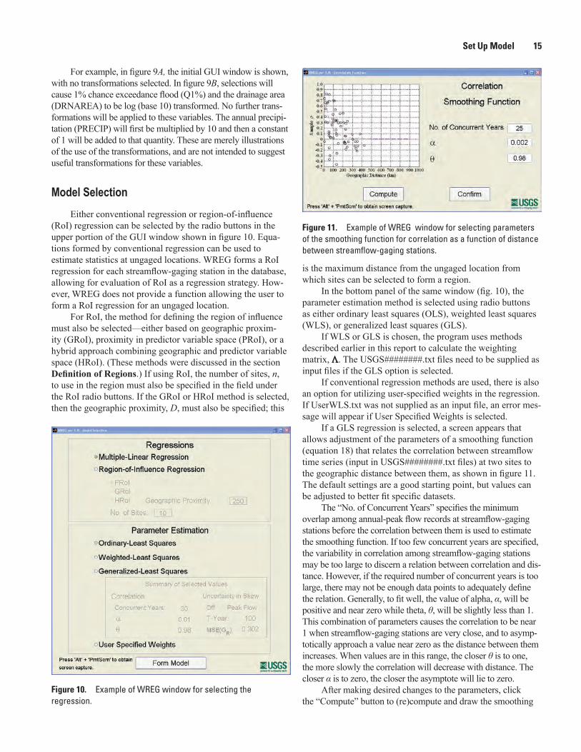
If a GLS regression is selected, a screen appears that allows adjustment of the parameters of a smoothing function (equation 18) that relates the correlation between streamflow time series (input in USGS########.txt files) at two sites to the geographic distance between them, as shown in figure 11. The default settings are a good starting point, but values can be adjusted to better fit specific datasets.

The “No. of Concurrent Years” specifies the minimum overlap among annual-peak flow records at streamflow-gaging stations before the correlation between them is used to estimate the smoothing function. If too few concurrent years are specified, the variability in correlation among streamflow-gaging stations may be too large to discern a relation between correlation and dis-tance. However, if the required number of concurrent years is too large, there may not be enough data points to adequately define the relation. Generally, to fit well, the value of alpha, α, will be positive and near zero while theta, θ, will be slightly less than 1. This combination of parameters causes the correlation to be near 1 when streamflow-gaging stations are very close, and to asymp-totically approach a value near zero as the distance between them increases. When values are in this range, the closer θ is to one, the more slowly the correlation will decrease with distance. The closer α is to zero, the closer the asymptote will lie to zero.

After making desired changes to the parameters, click the “Compute” button to (re)compute and draw the smoothing

For example, in figure 9A, the initial GUI window is shown, with no transformations selected. In figure 9B, selections will cause 1% chance exceedance flood (Q1%) and the drainage area (DRNAREA) to be log (base 10) transformed. No further trans-formations will be applied to these variables. The annual precipi-tation (PRECIP) will first be multiplied by 10 and then a constant of 1 will be added to that quantity. These are merely illustrations of the use of the transformations, and are not intended to suggest useful transformations for these variables.

Model SelectionEither conventional regression or region-of-influence

(RoI) regression can be selected by the radio buttons in the upper portion of the GUI window shown in figure 10. Equa-tions formed by conventional regression can be used to estimate statistics at ungaged locations. WREG forms a RoI regression for each streamflow-gaging station in the database, allowing for evaluation of RoI as a regression strategy. How-ever, WREG does not provide a function allowing the user to form a RoI regression for an ungaged location.

For RoI, the method for defining the region of influence must also be selected—either based on geographic proxim-ity (GRoI), proximity in predictor variable space (PRoI), or a hybrid approach combining geographic and predictor variable space (HRoI). (These methods were discussed in the section Definition of Regions.) If using RoI, the number of sites, n, to use in the region must also be specified in the field under the RoI radio buttons. If the GRoI or HRoI method is selected, then the geographic proximity, D, must also be specified; this

Figure 10. Example of WREG window for selecting the regression.

Figure 11. Example of WREG window for selecting parameters of the smoothing function for correlation as a function of distance between streamflow-gaging stations.


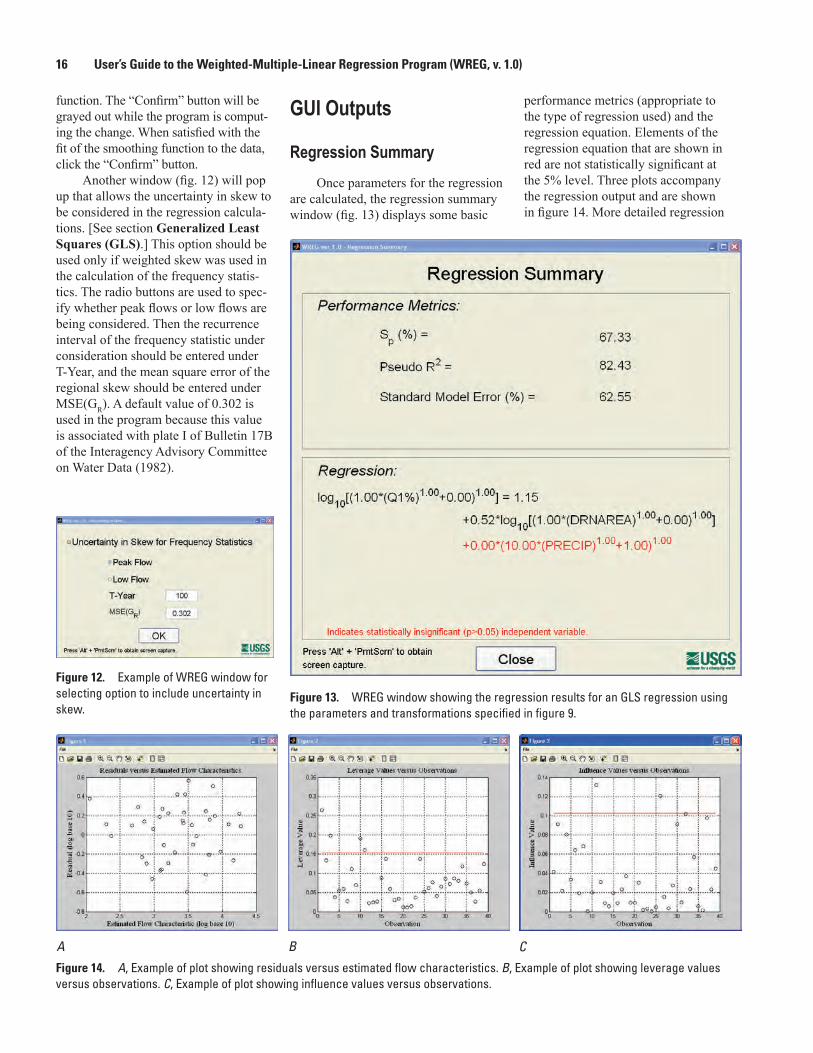
GUI Outputs

Regression SummaryOnce parameters for the regression

are calculated, the regression summary window (fig. 13) displays some basic

function. The “Confirm” button will be grayed out while the program is comput-ing the change. When satisfied with the fit of the smoothing function to the data, click the “Confirm” button.

Another window (fig. 12) will pop up that allows the uncertainty in skew to be considered in the regression calcula-tions. [See section Generalized Least Squares (GLS).] This option should be used only if weighted skew was used in the calculation of the frequency statis-tics. The radio buttons are used to spec-ify whether peak flows or low flows are being considered. Then the recurrence interval of the frequency statistic under consideration should be entered under T-Year, and the mean square error of the regional skew should be entered under MSE(GR). A default value of 0.302 is used in the program because this value is associated with plate I of Bulletin 17B of the Interagency Advisory Committee on Water Data (1982).

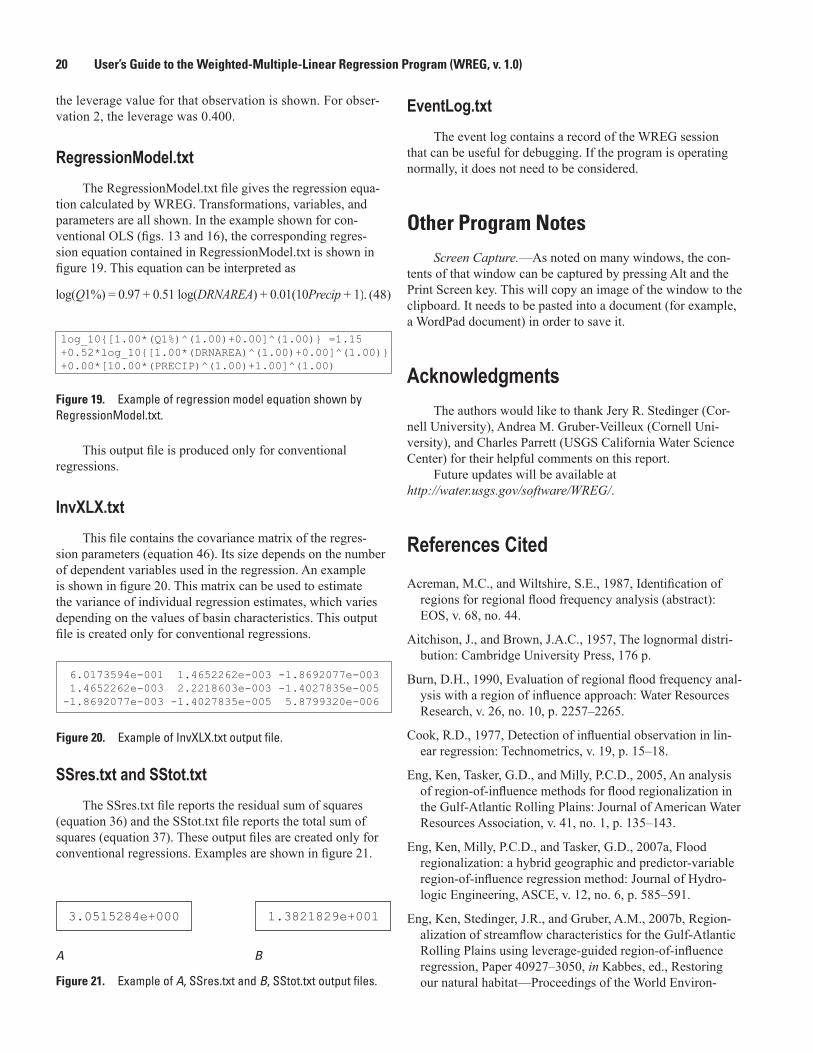
performance metrics (appropriate to the type of regression used) and the regression equation. Elements of the regression equation that are shown in red are not statistically significant at the 5% level. Three plots accompany the regression output and are shown in figure 14. More detailed regression

Figure 14. A, Example of plot showing residuals versus estimated flow characteristics. B, Example of plot showing leverage values versus observations. C, Example of plot showing influence values versus observations.

Figure 12. Example of WREG window for selecting option to include uncertainty in skew.

Figure 13. WREG window showing the regression results for an GLS regression using the parameters and transformations specified in figure 9.

Output Files 17

file can also be imported into a spreadsheet program, such as Microsoft Excel, as a text, tab-delimited file.

results, including p-values for individual parameters, are avail-able in the text output files.

Residuals Versus Estimated Flow CharacteristicsThis plot (fig. 14A) shows the regression residuals (equa-

tion 28) plotted against the estimated flow characteristics. Both axes will be in units of the transformed flow characteris-tics [for example, log (base 10)].

Leverage Values Versus ObservationsThis plot (figure 14B) shows the leverage values plot-

ted by observation number. Observations are numbered in the order in which they appear in the input files. The red line shows the threshold (as calculated by equation 41) above which an observation may be considered to have high lever-age, as calculated by the appropriate equation for the type of regression, discussed earlier in the section Leverage and Influence Statistic. Observations with high leverage should be checked carefully for possible errors.

Influence Values Versus ObservationsThis plot (fig. 14C) shows influence values plotted by

observation number. The red line shows the threshold (as calcu-lated by equation 45) above which an observation may be con-sidered to have large influence, as calculated by the appropriate equation for the type of regression, discussed earlier in the sec-tion Leverage and Influence Statistic. Observations with high influence should be checked carefully for possible errors.

Output FilesThe output files are listed in table 2 with a brief descrip-

tion. A detailed description of each file’s contents follows. A text editor can be used to view all of the output files. Each

Table 2. WREG output files.

File name DescriptionConventionalGLS.txt Results from a GLS regression.ConventionalOLS.txt Results from an OLS regression.ConventionalWLS.txt Results from a WLS regression.RegionofInfluenceOLS.txt Results from an OLS regression using RoI.RegionofInfluenceWLS.txt Results from a WLS regression using RoI.RegionofInfluenceGLS.txt Results from a GLS regression using RoI.RegressionModel.txt The regression equation (including transformations) calculated by WREG. Output only for conventional regression.InvXLX.txt Covariance of the regression parameters (equation 46). Output only for conventional regression.SSres.txt Residual sum of squares (equation 36). Output only for conventional regression.SStot.txt Total sum of squares (equation 37). Output only for conventional regression.EventLog.txt Record of the program’s execution. Helpful for diagnosing runtime errors.

NA

Regression Model for Q1%

Performance Metrics Mean Squared Error 0.085 R2 77.98 Standard Model Error*Note: R2 is in percent.

Coefficients of Model Std Error T value P>|T|

Constant DRNAREA 0.51 0.05 10.63 0.000PRECIP 0.01 0.00 2.54 0.015

Transformations C1 C2 C3 C4Q1% DRNAREA log10 1.00 1.00 0.00 1.00PRECIP 1 10.00 1.00 1.00 1.00

Residuals, Leverage, and Influence of Observations rage Limit 0.154

Influence Limit 0.103 Observation Residual Leverage Influence

1 0.145 0.216 0.0022 0.286 0.143 0.0053 0.108 0.200 0.0014 -0.622 0.028 0.0045 -0.333 0.045 0.0026 -0.435 0.053 0.0047 -0.322 0.028 0.0018 0.265 0.107 0.0039 -0.020 0.110 0.000

10 0.105 0.179 0.00111 0.346 0.183 0.01112 -0.385 0.034 0.00213 0.165 0.037 0.00014 -0.207 0.037 0.00115 -0.196 0.088 0.00116 0.069 0.125 0.00017 -0.269 0.056 0.00218 -0.407 0.033 0.00219 0.165 0.054 0.00120 0.210 0.042 0.001. . .

0.97 0.70 1.39 0.173

Leve

log10 1.00 1.00 0.00 1.00

Figure 15. Example of output file ConventionalOLS.txt. Residuals, leverage, and influence are shown only for the first 20 observations.


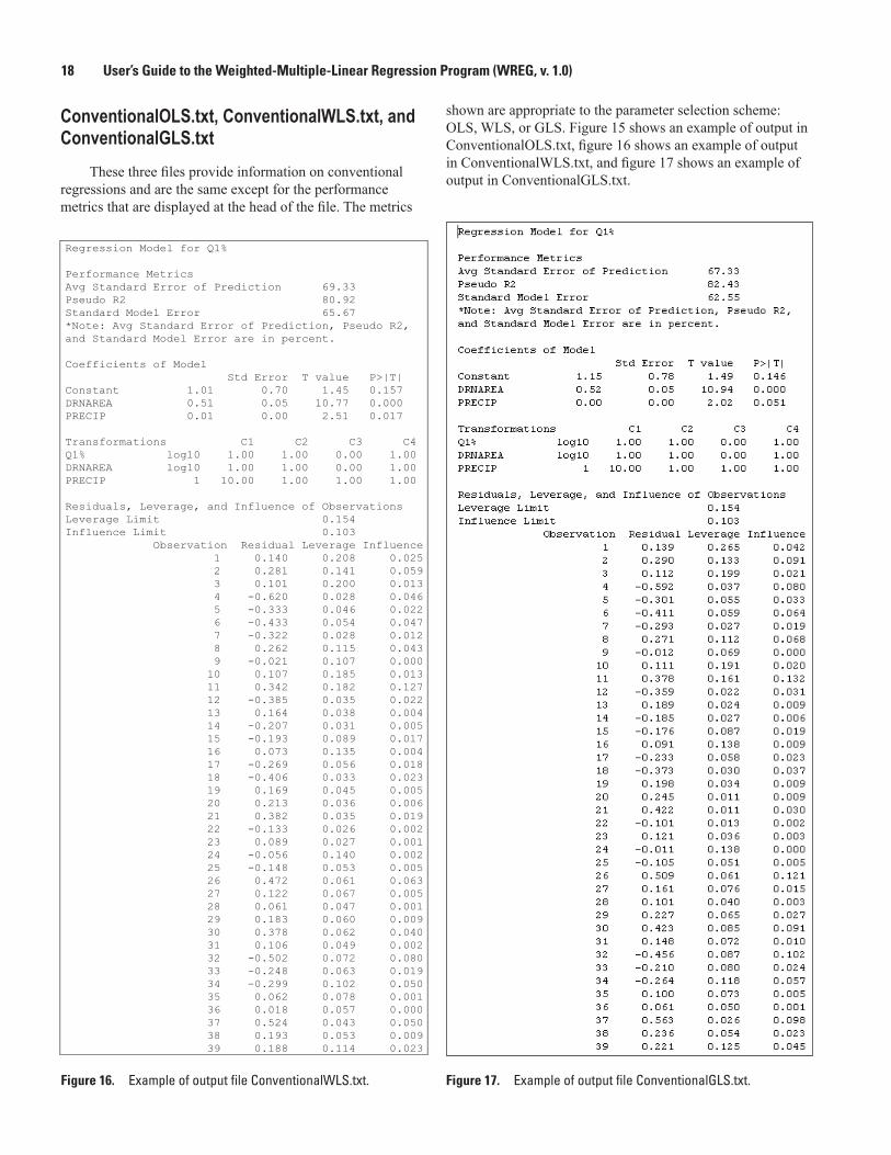
ConventionalOLS.txt, ConventionalWLS.txt, and ConventionalGLS.txt

These three files provide information on conventional regressions and are the same except for the performance metrics that are displayed at the head of the file. The metrics

shown are appropriate to the parameter selection scheme: OLS, WLS, or GLS. Figure 15 shows an example of output in ConventionalOLS.txt, figure 16 shows an example of output in ConventionalWLS.txt, and figure 17 shows an example of output in ConventionalGLS.txt.

Figure 17. Example of output file ConventionalGLS.txt.Figure 16. Example of output file ConventionalWLS.txt.

Regression Model for Q1% Performance Metrics Avg Standard Error of Prediction 69.33 Pseudo R2 80.92 Standard Model Error 65.67 *Note: Avg Standard Error of Prediction, Pseudo R2, and Standard Model Error are in percent. Coefficients of Model Std Error T value P>|T| Constant 1.01 0.70 1.45 0.157DRNAREA 0.51 0.05 10.77 0.000PRECIP 0.01 0.00 2.51 0.017 Transformations C1 C2 C3 C4Q1% log10 1.00 1.00 0.00 1.00DRNAREA log10 1.00 1.00 0.00 1.00PRECIP 1 10.00 1.00 1.00 1.00 Residuals, Leverage, and Influence of Observations Leverage Limit 0.154 Influence Limit 0.103 Observation Residual Leverage Influence 1 0.140 0.208 0.025 2 0.281 0.141 0.059 3 0.101 0.200 0.013 4 -0.620 0.028 0.046 5 -0.333 0.046 0.022 6 -0.433 0.054 0.047 7 -0.322 0.028 0.012 8 0.262 0.115 0.043 9 -0.021 0.107 0.000 10 0.107 0.185 0.013 11 0.342 0.182 0.127 12 -0.385 0.035 0.022 13 0.164 0.038 0.004 14 -0.207 0.031 0.005 15 -0.193 0.089 0.017 16 0.073 0.135 0.004 17 -0.269 0.056 0.018 18 -0.406 0.033 0.023 19 0.169 0.045 0.005 20 0.213 0.036 0.006 21 0.382 0.035 0.019 22 -0.133 0.026 0.002 23 0.089 0.027 0.001 24 -0.056 0.140 0.002 25 -0.148 0.053 0.005 26 0.472 0.061 0.063 27 0.122 0.067 0.005 28 0.061 0.047 0.001 29 0.183 0.060 0.009 30 0.378 0.062 0.040 31 0.106 0.049 0.002 32 -0.502 0.072 0.080 33 -0.248 0.063 0.019 34 -0.299 0.102 0.050 35 0.062 0.078 0.001 36 0.018 0.057 0.000 37 0.524 0.043 0.050 38 0.193 0.053 0.009 39 0.188 0.114 0.023

Output Files 19

The observations are the observed flow characteristic (dependent variable) at each streamflow-gaging station and are numbered in ascending order, as the stations appear in the FlowChar.txt file (and other files).

RegionofInfluenceOLS.txt, RegionofInfluenceWLS.txt, and RegionofInfluenceGLS.txt

These three files show the same outputs but are produced using OLS, WLS, or GLS. The example shown in figure 18 is for RoI using OLS regression (RegionofInfluenceOLS.txt). This file provides information on the results of the RoI regression, and can be used to gauge whether an RoI regression may provide suitable results. However, WREG does not include a function that would allow users to perform a RoI regression at an ungaged loca-tion. The results shown by WREG are solely for demonstra-tion or evaluation purposes.

WREG forms an individual RoI regression for each streamflow-gaging station included in the input dataset. The first several lines of the file show overall performance met-rics for the RoI regression, when each of these individual

regressions are considered. Next, the coefficients of the RoI regression built for each site in the dataset are shown. If 200 sites are included in the dataset, 200 results will be shown—one for each regression that was built. These individual regres-sions will be numbered 1 to 200, and reflect the numerically ascending order of the Station IDs. That is, the Station ID with the smallest number would be associated with regression 1 or observation 1 in this output file and the Station ID with the largest number would be associated with the regression 200 or observation 200 in this output file.

The output file next displays the transformations that were used in the regressions. WREG does not allow differ-ent transformations to be used for different RoI regressions, and a single transformation applies to all individual RoI regressions formed by WREG. Next, the PRESS-like MSE of the RoI residuals are shown for the regression formed for each site in the dataset. Finally, the output file displays information on leverage and influence. For each regression, the output shows the observations that were used to form the regression as well as the leverage calculated for that observa-tion. These outputs are paired. For example, in output shown in figure 18, the first regression used observations 2, 8, 3, 9, 14, 13, 12, 7, 10, and 5. Following each observation number,

Figure 18. Example of output file RegionofInfluenceOLS.txt.

Region-of-Influence Regression Models for Q1% Performance Metrics Root Mean Square Error 73.45 Pseudo R2 NA Standard Model Error NA *Note: Root Mean Square Error is in percent. Coefficients of Model Regression Constant Coefficients DRNAREA PRECIP 1 4.61 0.54 -0.01 2 3.84 0.54 -0.00 3 4.10 0.29 -0.00 4 -2.65 0.60 0.02 5 2.97 0.30 -0.00 6 -1.28 0.70 0.01 . . . Transformations C1 C2 C3 C4 Q1% log10 1.00 1.00 0.00 1.00 DRNAREA log10 1.00 1.00 0.00 1.00 PRECIP 1 10.00 1.00 1.00 1.00 PRESS_RoI Residuals Observation Residual 1 0.060 2 0.028 3 0.141 4 0.262 5 0.047 6 0.132 . . . Leverage and Influence Leverage Limit 0.400 Influence Limit NA Regression Observations Included in RoI Model and Leverage Value 1 2 0.400 8 0.293 3 0.461 9 0.184 14 -0.038 13 -0.046 12 -0.075 7 -0.163 10 0.149 5 -0.165 2 1 0.315 8 0.169 3 0.356 13 0.050 14 0.020 12 0.035 9 0.054 7 -0.012 5 0.035 18 -0.020 3 2 0.385 1 0.445 8 0.112 11 0.518 13 -0.081 12 -0.113 5 -0.046 14 -0.202 17 -0.041 35 0.024 4 23 0.096 22 0.106 7 0.083 14 0.099 20 0.120 6 0.133 12 0.080 18 0.070 19 0.133 13 0.079 5 17 0.249 18 0.068 35 0.327 12 0.141 7 0.031 13 0.172 36 0.033 25 -0.080 32 0.023 14 0.035 6 15 0.159 19 0.098 4 0.073 20 0.077 22 0.062 14 0.086 23 0.051 16 0.174 9 0.172 7 0.047 . .

.


EventLog.txtThe event log contains a record of the WREG session

that can be useful for debugging. If the program is operating normally, it does not need to be considered.

Other Program NotesScreenCapture.—As noted on many windows, the con-

tents of that window can be captured by pressing Alt and the Print Screen key. This will copy an image of the window to the clipboard. It needs to be pasted into a document (for example, a WordPad document) in order to save it.

AcknowledgmentsThe authors would like to thank Jery R. Stedinger (Cor-

nell University), Andrea M. Gruber-Veilleux (Cornell Uni-versity), and Charles Parrett (USGS California Water Science Center) for their helpful comments on this report.

Future updates will be available at http://water.usgs.gov/software/WREG/.

References CitedAcreman, M.C., and Wiltshire, S.E., 1987, Identification of

regions for regional flood frequency analysis (abstract): EOS, v. 68, no. 44.

Aitchison, J., and Brown, J.A.C., 1957, The lognormal distri-bution: Cambridge University Press, 176 p.

Burn, D.H., 1990, Evaluation of regional flood frequency anal-ysis with a region of influence approach: Water Resources Research, v. 26, no. 10, p. 2257–2265.

Cook, R.D., 1977, Detection of influential observation in lin-ear regression: Technometrics, v. 19, p. 15–18.

Eng, Ken, Tasker, G.D., and Milly, P.C.D., 2005, An analysis of region-of-influence methods for flood regionalization in the Gulf-Atlantic Rolling Plains: Journal of American Water Resources Association, v. 41, no. 1, p. 135–143.

Eng, Ken, Milly, P.C.D., and Tasker, G.D., 2007a, Flood regionalization: a hybrid geographic and predictor-variable region-of-influence regression method: Journal of Hydro-logic Engineering, ASCE, v. 12, no. 6, p. 585–591.

Eng, Ken, Stedinger, J.R., and Gruber, A.M., 2007b, Region-alization of streamflow characteristics for the Gulf-Atlantic Rolling Plains using leverage-guided region-of-influence regression, Paper 40927–3050, in Kabbes, ed., Restoring our natural habitat—Proceedings of the World Environ-

the leverage value for that observation is shown. For obser-vation 2, the leverage was 0.400.

RegressionModel.txtThe RegressionModel.txt file gives the regression equa-

tion calculated by WREG. Transformations, variables, and parameters are all shown. In the example shown for con-ventional OLS (figs. 13 and 16), the corresponding regres-sion equation contained in RegressionModel.txt is shown in figure 19. This equation can be interpreted as

. (48)

This output file is produced only for conventional regressions.

InvXLX.txtThis file contains the covariance matrix of the regres-

sion parameters (equation 46). Its size depends on the number of dependent variables used in the regression. An example is shown in figure 20. This matrix can be used to estimate the variance of individual regression estimates, which varies depending on the values of basin characteristics. This output file is created only for conventional regressions.

SSres.txt and SStot.txtThe SSres.txt file reports the residual sum of squares

(equation 36) and the SStot.txt file reports the total sum of squares (equation 37). These output files are created only for conventional regressions. Examples are shown in figure 21.

Figure 19. Example of regression model equation shown by RegressionModel.txt.

log_10{[1.00*(Q1%)^(1.00)+0.00]^(1.00)} =1.15 +0.52*log_10{[1.00*(DRNAREA)^(1.00)+0.00]^(1.00)} +0.00*[10.00*(PRECIP)^(1.00)+1.00]^(1.00)

6.0173594e-001 1.4652262e-003 -1.8692077e-003 1.4652262e-003 2.2218603e-003 -1.4027835e-005 -1.8692077e-003 -1.4027835e-005 5.8799320e-006

Figure 20. Example of InvXLX.txt output file.

Figure 21. Example of A, SSres.txt and B, SStot.txt output files.

3.0515284e+000 1.3821829e+001

http://water.usgs.gov/software/WREG/

http://water.usgs.gov/software/WREG/

References Cited 21

mental and Water Resources Congress, May 15–18, 2007, Tampa, Florida: American Society of Civil Engineers.

Funkhouser, J.E., Eng, Ken, and Moix, M.W., 2008, Low-flow characteristics for selected streams and regionalization of low-flow characteristics in Arkansas: U.S. Geological Survey Scientific Investigations Report 2008–5065, 161 p., available only online at http://pubs.usgs.gov/sir/2008/5065/. (Accessed August 19, 2009.)

Giese, G.L., and Mason, R.R., Jr., 1993, Low-flow character-istics of streams in North Carolina: U.S. Geological Survey Water Supply Paper 2403, 29 p., 2 plates. (Also available online at http://pubs.er.usgs.gov/usgspubs/wsp/wsp2403.)

Griffis, V.W., and Stedinger, J.R., 2007, The use of GLS regression in regional hydrologic analyses: Journal of Hydrology, v. 344, p. 82–95.

Griffis, V.W., and Stedinger, J.R., 2009, Log-Pearson type 3 distribution and its application in flood frequency analysis. III: sample skew and weighted skew estimators: Journal of Hydrologic Engineering, v. 14, no. 2, p. 121–130.

Hardison, C.H., 1971, Prediction error of regression estimates of streamflow characteristics at ungaged sites: U.S. Geolog-ical Survey Professional Paper 750–C, p. c228–c236. (Also available at http://pubs.er.usgs.gov/usgspubs/pp/pp750C.) (Accessed August 19, 2009.)

Hirsch, R.M., 1982, A comparison of four streamflow record extension techniques: Water Resources Research, v. 18, no. 4, p. 1081–1088.

Interagency Advisory Committee on Water Data, 1982, Guidelines for determining flood-flow frequency, Bulletin 17B of the Hydrology Subcommittee, Office of Water Data Coordination: U.S. Geological Survey, Reston, Va., 183 p. (Also available at http://water.usgs.gov/osw/bulletin17b/dl_flow.pdf.) (Accessed August 19, 2009.)

Kenney, T.A., Wilkowske, C.D., and Wright, S.J., 2007, Methods for estimating magnitude and frequency of peak flows for natural streams in Utah: U.S. Geological Survey Scientific Investigations Report 2007–5158, 28 p. (Version 4.0 was released March 10, 2008, and is available only online at http://pubs.usgs.gov/sir/2007/5158/.) (Accessed August 19, 2009.)

Kite, G.W., 1975, Confidence limits for design events: Water Resources Research, v. 11, no. 1, p. 48–53.

Kite, G.W., 1976, Reply to comment on Confidence limits for design events: Water Resources Research, v. 12, no. 4, p. 826.

Martins, E.S., and Stedinger, J.R., 2002, Cross correlations among estimators of shape: Water Resources Research, v. 38, no. 11, p. 34-1–34-7, doi:10.1029/2002WR001589.

Merz, R., and Blöschl, G., 2005, Flood frequency regionalisa-tion—spatial proximity vs. catchment attributes: Journal of Hydrology, v. 302, p. 283–306.

Montgomery, D.C., Peck, E.A., and Vining, G.G., 2001, Intro-duction to linear regression analysis (3d ed.): New York, John Wiley and Sons, 641 p.

Neely, B.L., Jr., 1986, Magnitude and frequency of floods in Arkansas: U.S. Geological Survey Water Resources Inves-tigations Report 86–4335, 51 p., available only online at http://pubs.er.usgs.gov/usgspubs/wri/wri864335/. (Accessed August 19, 2009.)

Ries, K.G., III, and Fries, 2000, Methods for estimating low-flow statistics for Massachusetts streams: U.S. Geo-logical Survey Water-Resources Investigations Report 2000-4135, 81p. (Also available at http://pubs.usgs.gov/wri/wri004135/.) (Accessed August 24, 2009.)

Ries, K.G., III, comp., 2007, The National Streamflow Statistics Program: A computer program for estimating streamflow statistics for ungaged sites: U.S. Geological Survey Techniques and Methods book 4, chap. A6, 45 p. (Also available at http://pubs.usgs.gov/tm/2006/tm4a6/.) (Accessed August 19, 2009.)

Stedinger, J.R., and Tasker, G.D., 1985, Regional hydro-logic analysis, 1, ordinary, weighted, and generalized least squares compared: Water Resources Research, v. 21, no. 9, p. 1421–1432.

Stedinger, J.R., and Tasker, G.D., 1986, Regional hydrologic analysis, 2, model-error estimators, estimation of sigma and log-Pearson Type 3 distributions: Water Resources Research, v. 22, no. 10, p. 1487–1499.

Tasker, G.D., 1980, Hydrologic regression with weighted least squares: Water Resources Research, v. 16, no. 6, p. 1107–1113.

Tasker, G.D., and Stedinger, J.R., 1986, Regional skew with weighted LS regression: Journal of Water Resources Plan-ning and Management, ASCE, v. 112, no. 2, p. 225–236.

Tasker, G.D., and Stedinger, J.R., 1989, An operational GLS model for hydrologic regression: Journal of Hydrology, v. 111, p. 361–375.

Tasker, G.D., Hodge, S.A., and Barks, C.S., 1996, Region of influence regression for estimating the 50-year flood at ungaged sites: Water Resources Bulletin, v. 32, no. 1, p. 163–170.

Thomas, D.M., and Benson, M.A., 1970, Generalization of streamflow characteristics from drainage-basin character-istics: U.S. Geological Survey Water-Supply Paper 1975, 55 p. (Also available online at http://pubs.er.usgs.gov/usgspubs/wsp/wsp1975.) (Accessed August 19, 2009.)

Wandle, S.W., 1977, Estimating the magnitude and fre-quency of floods on natural-flow streams in Massachusetts: U.S. Geological Survey Water-Resources Investigations Report 77–39, 26 p., 1 plate. (Also available online at http://pubs.er.usgs.gov/usgspubs/wri/wri7739.)

http://pubs.usgs.gov/sir/2008/5065/

http://pubs.er.usgs.gov/usgspubs/wsp/wsp2403

http://pubs.er.usgs.gov/usgspubs/pp/pp750C

http://water.usgs.gov/osw/bulletin17b/dl_flow.pdf

http://water.usgs.gov/osw/bulletin17b/dl_flow.pdf

http://pubs.usgs.gov/sir/2007/5158/

http://pubs.er.usgs.gov/usgspubs/wri/wri864335

http://pubs.usgs.gov/wri/wri004135/

http://pubs.usgs.gov/wri/wri004135/

http://md.water.usgs.gov/publications/tm-4-a6/

http://md.water.usgs.gov/publications/tm-4-a6/

http://pubs.usgs.gov/tm/2006/tm4a6/



http://pubs.er.usgs.gov/usgspubs/wri/wri7739

Eng, Chen, and Kiang—U

ser’s Guide to the W

eighted-Multiple-Linear Regression Program

(WREG

version 1.0)—Techniques and M

ethods 4–A8

user’s guide to the weighted-multiple-linear …. department of the interior u.s. geological...

Documents