users guide to initial findings - university college london
TRANSCRIPT

Millennium Cohort Study
Second Survey
A User’s Guide to Initial Findings
Edited by
Kirstine Hansen and Heather Joshi
July 2007
Centre for Longitudinal Studies
Bedford Group for Lifecourse and Statistical Studies Institute of Education, University of London

This edition dated 20 July 2007 contains a few corrections over the previous version posted on 11th June 2007, by the: Centre for Longitudinal Studies Bedford Group for Lifecourse and Statistical Studies Institute of Education, University of London 20 Bedford Way London WC1H 0AL Website: www.cls.ioe.ac.uk © Centre for Longitudinal Studies ISBN 1 898453 60 8 The Centre for Longitudinal Studies (CLS) is one of six centres that comprise the Bedford Group for Lifecourse and Statistical Studies (www.ioe.ac.uk/bedfordgroup). CLS is devoted to the collection, management and analysis of large-scale longitudinal data. It has responsibility for Britain's internationally renowned birth cohort studies, the National Child Development Study (1958 cohort) and the 1970 British Cohort Study, and leads the consortium conducting the ESRC's Millennium Cohort Study. The views expressed in this work are those of the authors and do not necessarily reflect the views of the Economic and Social Research Council or the Office for National Statistics. All errors and omissions remain those of the authors.

CONTENTS List of contributors Acknowledgements Executive summary 1. Introduction Kirstine Hansen and Heather Joshi 2. Housing, neighbourhood and community Gareth Hughes, Sosthenes Ketende and Ian Plewis 3. Family demographics and relationships Lisa Calderwood 4. Grandparents Denise Hawkes and Heather Joshi 5. Parenting Kate Smith 6. Child health
Carol Dezateux, Alice Sullivan, Summer Sherburne Hawkins, Tim Cole and Heather Joshi
7. Child behaviour and cognitive development Anitha George, Kirstine Hansen and Ingrid Schoon 8. Parental health and lifestyle Lisa Calderwood, Yvonne Kelly and Lidia Panico 9. Parental employment Kelly Ward and Shirley Dex 10. Income and poverty Kelly Ward, Alice Sullivan and Jonathan Bradshaw 11. Childcare Anitha George and Kirstine Hansen 12. Older siblings Ian Plewis 13. Conclusions Kirstine Hansen and Heather Joshi

LIST OF CONTRIBUTORS NAME
TITLE INSTITUTION
Jonathan Bradshaw Professor of Social Policy University of York
Lisa Calderwood Millennium Cohort Study Survey Manager
Centre for Longitudinal Studies, Institute of Education, University of London
Tim Cole Professor of Medical Statistics
Institute of Child Health, University College London
Carol Dezateux Professor of Paediatric Epidemiology
Institute of Child Health
Shirley Dex Professor of Longitudinal Social Research
Centre for Longitudinal Studies
Anitha George Research Officer Centre for Longitudinal Studies
Kirstine Hansen Research Director: Millennium Cohort Study
Centre for Longitudinal Studies
Denise Hawkes Research Officer Centre for Longitudinal Studies Gareth Hughes Research Officer Centre for Longitudinal Studies
Heather Joshi Director: Centre for Longitudinal Studies
Centre for Longitudinal Studies,
Yvonne Kelly Lecturer in Epidemiology and Public Health
Department of Epidemiology, University College London
Sosthenes Ketende Research Officer Centre for Longitudinal Studies
Lidia Panico Research Officer Department of Epidemiology, University College London
Ian Plewis Professor of Longitudinal Research Methods
Centre for Longitudinal Studies
Ingrid Schoon Professor of Psychology City University
Summer Sherburne Hawkins
Dept of Health funded Researcher
Institute of Child Health
Kate Smith Millennium Cohort Study Survey Manager
Centre for Longitudinal Studies
Alice Sullivan Research Officer Centre for Longitudinal Studies
Kelly Ward Research Officer Centre for Longitudinal Studies

ACKNOWLEDGEMENTS We are grateful for the co-operation of the children who form the Millennium Birth Cohort and their mothers, fathers and other family members, all entirely voluntary. We wish to acknowledge the initiation and funding of the survey by the Economic and Social Research Council, and its substantial supplementation by the consortium, led by the Office for National Statistics (ONS), of government departments: the Department for Education and Skills, the Department of Work and Pensions, the Department of Health and the governments of Wales, Scotland and Northern Ireland. The National Evaluation of the Children’s Fund offered the opportunity to enhance the second survey in several ways, as did the International Centre for Child Studies. The work could not have been accomplished without the involvement of a large number of advisers drawn from academics, policy-makers and funders, who we consulted throughout the design of the surveys. Particular thanks go to those who served on the MCS Advisory Committee and the MCS Advisory Groups for the second survey. The survey and this document also benefited from the enthusiasm and expertise of: • Researchers, programmers, field-managers and interviewers at NOP, and their
sub-contractors, Millward Brown in Northern Ireland. • The staff of the Newcastle Information Centre of HM Revenue and Customs,
formerly the Department of Social Security • The members of the CLS tracing team, IT team, communications team, database
team, survey and research teams. The production of this report has been funded by the ONS-led consortium of government departments. We are grateful to members of their staff who have made comments on this report.
1

The Millennium Cohort Study Internal Team (CLS) The following team contributed to the second survey of the MCS: Prof Heather Joshi, Study Director Dr Kirstine Hansen, Research Director and Deputy Study Director Chris Baker, Administrator Denise Brown, Cohort Relations Robert Browne, Database Manager Lisa Calderwood, Survey Manager Prof Shirley Dex Peter Deane, Tracing Team Kevin Dodwell, Tracing Team, Anitha George, Research Officer Dr Denise Hawkes, Research Officer Gareth Hughes, Research Officer Jon Johnson, Senior Database Manager Sosthenes Ketende, Research Officer Tiziana Leone, Research Officer Mary Londra, Survey Officer Suzanna Mouzo, Tracing Team Prof Ian Plewis, Director of Methodology Rachel Rosenberg, Data Officer Peter Shepherd, Director of Survey Operations Kate Smith, Survey Manager Dr Alice Sullivan, Research Officer Mina Thompson, Administrator Kelly Ward, Research Officer Members of the Research Collaborators’ Team Prof Mel Bartley, University College London Dermot Bowler, City University, London Dr Helen Bedford, Institute of Child Health, Prof Julia Brannen, Institute of Education Prof John Bynner, Institute of Education Prof Tim Cole, Institute of Child Health Dr Leslie Davidson, Columbia University Prof Carol Dezateux, Institute of Child Health Dr Elsa Ferri, Institute of Education Dr Leon Feinstein, Institute of Education Dr Yvonne Kelly, University College London Prof Kathleen Kiernan, London School of Economics Prof Alison Macfarlane, City University Prof Sir Michael Marmot, University College London Dr Barbara Maughan, Institute of Psychiatry Prof Catherine Peckham, Institute of Child Health Prof Christine Power, Institute of Child Health Prof Ingrid Schoon, City University Dr Marjorie Smith, Institute of Education We are also indebted to Professor Neville Butler, who died in February 2007. Founder of the 1958 and 1970 British Cohort Studies and an ardent supporter of the Millennium Cohort Study, he inspired and supported the MCS survey team up until the final year of his life. We dedicate this publication to him.
2

Fieldwork Contractors NOP World Nick Moon Claire Ivins Nickie Rose Nikki Steel
3

EXECUTIVE SUMMARY This report presents some of the main initial findings of the Second Survey of the Millennium Cohort Study conducted by the Centre for Longitudinal Studies, which is based at the Institute of Education, University of London. It is intended to provide an introduction to potential users of the survey and to stimulate further in-depth and longitudinal analysis. 1. Introduction The second sweep of the Millennium Cohort Study (MCS2) collected information from 15,590 families of children born across the UK in 2000-2 when they reached the age of three. Almost all of these families (14,898) had been in the first survey when the children were nine-months-old. An additional 692 families were recruited for the second survey in England who had been eligible for the first survey but not included. The study’s first sweep, carried out during 2001-2, laid the foundations for this major new longitudinal research resource, involving a year-long cohort of around 19,000 babies. It recorded the circumstances of pregnancy and birth, the all-important early months of life, and the social and economic backgrounds of the families into which the children were born. The second survey data allow researchers for the first time to chart the changing circumstances of these children and their families and offer some direct measurements of the children’s development at the age of three which can be related to their earlier experiences. The sample was designed to provide adequate numbers from areas with high proportions of minority-ethnic residents (in England) and high child poverty, as well as the three smaller countries of the UK. This does not necessarily yield adequate samples of all minority ethnic groups, especially those not living in the sort of areas that were over-sampled, such as the Chinese. In most of the tables, as noted in them, the numbers analysed exclude some cases with insufficient information or in small categories that would require different treatment, such as families where the child is not living with their mother or is a twin or triplet. Percentages reported here are re-weighted to provide representative estimates. Attention is drawn to differences among them if statistically significant. Note also that behind the averages and proportions lie the individual differences between every child. To say, for example, that girls are ahead of boys for a particular indicator like vocabulary, on average, does not mean that all girls are ahead of all boys. It would also be quite wrong to suggest that all children from a particular disadvantaged background are destined to fail. What the survey is setting out to do is chart the risks that threaten to limit the achievements of a new generation. 2. Housing, neighbourhood and community Moving home is often an important event in the lives of families with young children. Over one-third of the sample from sweep 1 (38 per cent) had changed address in the intervening 27 or so months. Families in Scotland had moved the longest distance on average (35 kms) whereas families in Northern Ireland had moved the shortest distance (11 kms). Most families had not moved far, however, and many had found
4

other homes in the same neighbourhood. Very few survey members had left the UK or moved from one UK country to another between the surveys. Almost half the families who had moved had done so because they wanted a bigger home (47.2 per cent) while nearly a quarter (22.7 per cent) said they had wanted to move into a better area. Sweep 2 confirmed that mobility is socially and geographically patterned. It is more common in Scotland than in Northern Ireland; less common in families with a South Asian background; and more common in the groups that were lower-income, flat-dwelling and renting at the time of sweep 1. The main survey respondents in Northern Ireland were particularly positive about their home area in terms of bringing up children and feeling safe. They also reported a calmer atmosphere in the home, as did Indian families. White and Indian families were also more likely to describe their area as excellent for bringing up children. Black ethnic groups, however, were least likely to consider their area ‘very safe’. 3. Family demographics and relationships This chapter presents a picture of both change and stability in the membership of the cohort families. By MCS2 just over a quarter of the children had gained a younger brother or sister, and there had been comings and goings among the parents with whom they lived. In around 6 per cent of families interviewed for both surveys, two parents had parted company. A further 3 per cent headed by a single parent at sweep 1 had since gained a second parent. Well over half the ‘new’ parents were the child’s natural father who had not been living in the same home as the child at sweep 1. Among natural fathers who were not living with the child at sweep 2, two-thirds were reported to be in some form of contact. More than half (56 per cent) of the absent fathers made some maintenance payments. There were also signs of stabilisation in family life. The proportion of couples who were legally married went up, and the vast majority of the cohort families still comprised two natural parents. At age three, 15 per cent of the families were headed by lone mothers. This is much the same rate as at sweep 1, but with some turnover noted above and differential loss of families who had only one parent at sweep 1. Wales had the highest proportion of lone natural-mother families at both sweeps while Northern Ireland had the highest proportion of married natural-parent families. Lone parenthood was far more common among younger mothers aged 16 to 24 (42.5 per cent) than 35 to 39-year-olds (8.1 per cent). Only a fifth of younger mothers were married to the child’s father, but a quarter were cohabiting with him. Black Caribbean families had a far higher proportion of lone mothers (46.6 per cent) than White (14.3 per cent) or Indian (5 per cent) families. Family size also varied substantially by ethnic group. Cohort children in Bangladeshi families were most likely to have three or more siblings (32.6 per cent) while White (8 per cent), Mixed (8 per cent) and Indian children (4.8 per cent) were least likely.
5

4. Grandparents Almost all the cohort children had at least one living grandparent at sweep 2. Twenty-five per cent of the children had had some form of childcare from a grandparent and 90 per cent of cohort families had received financial support from grandparents. Over 80 per cent of the grandparents had been born in the UK. Those who had not were most likely to have come from Pakistan, India, Ireland and Bangladesh (about 6 per cent of the cohort’s parents were second-generation immigrants who had been born in the UK). Although few families included resident grandparents (4 per cent), in many cases the two generations of parents saw a lot of each other. For example, 65 per cent of mothers whose own mothers were alive saw them at least weekly and one-fifth saw them daily. Interestingly, the children of working mothers who had been looked after by a grandparent at nine months showed similar levels of linguistic development to those who had been in early formal childcare settings. On average, they had almost as high a vocabulary score as those who had attended formal care and they were clearly ahead of those who had been cared for by the father or had received another type of informal care while their mother had been working. Assessments of the children’s ‘school readiness’ (which measured their understanding of concepts such as colours, letters, numbers/counting, sizes, comparisons and shapes) put infants with grandparent care a little further behind those who had been in formal care. However, they were still ahead of those who had experienced other types of informal care.
5. Parenting The study provides a rich resource to look at different aspects of parenting, particularly in relation to fathers. Both parents (where there were two living with the child) were asked a wide range of questions regarding their activities and behaviours with their children and their different parenting styles and beliefs. Their responses provide a unique picture of what parents were doing with their children at the age of three, and how well they felt they were managing as parents. There are many similarities in parenting practice and beliefs between mothers and fathers. There are also common features across types of families, distinguished here by: country in the UK, ethnic group, age at interview and family employment status. Working mothers were less likely to feel they had enough time with their child, but on most other measures of parenting, they were no different from other mothers. In fact, two-earner couples were most likely to read to their child regularly. This provides indirect evidence that maternal employment does not eliminate ‘quality time’ with the child. Employed fathers, who were more likely than employed mothers to be working full-time and for long hours, were most likely to feel that they did not have enough time with their child. Fathers in general were less likely to report reading every day to their child than were mothers, but, if anything, it was fathers in families with no parent in paid work who were least likely to get involved in reading. Otherwise there was little difference in the parenting behaviour of fathers with or without jobs. Fathers in
6

Wales, however, were most likely to say they never read to their children (7 per cent) while Scots fathers were least likely to say this (3 per cent). There were also clear differences in parenting style across different groups of mothers and fathers, whether employed or not. For example, Black Caribbean mothers were most likely to report that they had lots of rules (39 per cent) compared to 17 per cent of Bangladeshi mothers, who were the least likely. However, these two groups were both markedly more likely than average to rate themselves very good mothers (65 per cent of Bangladeshi and 42 per cent of Black Caribbean mothers, compared with the UK average of only 31 per cent). Virtually all mothers said they wanted to impart such values as independence, obedience and respect. But mothers in Northern Ireland were keener to instil religious values in their children than mothers in the other UK countries. Eighty-five per cent of Northern Irish mothers considered religious values important, compared with just over half in England, Wales and Scotland. Pakistani and Black African mothers (98 and 96 per cent) also regarded religious values as important whereas only half of White mothers did (54 per cent). There was also an age divide. Older mothers wanted their children to adopt religious values (64 per cent of 35 to 39-year-olds) but only a minority of 16 to 24-year-old mothers (38 per cent) felt they were important. It will be interesting to discover whether these systematic and individual differences in parenting styles and attitudes will change as the child gets older and whether they will be related to behaviour and achievement later on. This is something that MCS data will be able to reveal in the future. 6. Child health This preliminary look at the health data collected by sweep 2 suggests that while the majority of pre-school children in the four UK countries were healthy, a minority were in poor health. One in six had a longstanding illness. The survey also showed that children starting out in disadvantaged communities were more likely to suffer disability and ill health, and to experience more problems with vision and hearing, as well as asthma and other longstanding conditions, chronic infections and injuries. However, there is no systematic tendency for poor health among children starting out or living in areas with a high proportion of minority-ethnic residents. This perhaps reflects ethnic diversity in health–related behaviours such as breastfeeding and parental smoking. One-quarter of the cohort children were either overweight or obese (5 per cent obese). Children in disadvantaged areas were a little more likely to be overweight and obese. However, the highest proportion of overweight (but not obese) children was found in the more advantaged areas of Wales. Indian children were least likely to be overweight or obese (9.2 per cent) while Black Caribbean infants were most likely to be too heavy for their age (32.5 per cent). There were no statistically significant differences in obesity between boys and girls.
7

Some early and important gender differences were, however, observed in other areas. Boys were more likely to be delayed in toilet training and speech, to have suffered from wheezing and asthma and to have required medical attention for injuries. Girls were more likely to have had chickenpox and to have received the combined MMR vaccine. These variations may relate to different social expectations and early social experiences and may in turn influence access to early-years provision and later health. 7. Cognitive development and behaviour The survey pioneered the mass collection of data on three-year-olds’ cognitive skills in their own home. Two established assessments were used: the Naming Vocabulary Subtest of the British Ability Scales and the School Readiness Composite (SRC) of the Revised Bracken Basic Concept Scale. The first is part of a set of cognitive assessments designed to assess children’s expressive language skills. The SRC consists of six tests that measure ‘readiness’ for formal education by assessing knowledge of colours, letters, numbers/counting, sizes, comparisons and shapes. Both assessments were administered by survey team members in computer-assisted interviews. The results show marked differences between children from advantaged and disadvantaged backgrounds. Better cognitive scores were achieved by children from families with two working parents who were highly educated and had higher incomes. The vocabulary assessment revealed that girls had marginally better expressive language skills than boys. Children in Scotland were ahead of those in the rest of the UK by about two months, which represents about three months of development at this age. Scots children and girls also did well in the school readiness assessment. The lead in average scores in Scotland is equivalent to about two months’ progress while girls, on average, are three months ahead of boys. Ethnic differences also appeared to be marked, with Bangladeshi and Pakistani children recording relatively low scores. The vocabulary assessment results, taken at face value, would represent a severe delay for the Bangladeshi and Pakistani children. Their scores were well below those normally expected for two-and-a-half-year-olds, let alone those aged over three, as these were. This is despite the fact that the assessment was not offered to non-English-speaking children. Before drawing firm conclusions about how to interpret this finding, it will be necessary to investigate the circumstances in which the assessments were and were not done, allowing for whether they lived in homes where English was not the main language spoken, which could slow their development of English vocabulary. There may also be cultural differences in the children’s readiness to attempt the task or engage with an unfamiliar visitor. Similar patterns were found in the school readiness results: Bangladeshi boys were the lowest scorers and White girls the highest. Bangladeshi children’s school readiness scores, again taken at face value, were about one year behind those of White children, and Pakistani children’s scores fell short of White children’s by eleven months for boys and 10 months for girls. Again, many factors may be contributing to this gap, and this assessment may therefore not be a fair indicator of these children’s
8

current or future ability. The same can be said of other differences that the assessment highlighted. Although only 4 per cent of the White children had scores in the ‘delayed’ range, over one quarter of the Black African and Black Caribbean children, as well as the Bangladeshi and Pakistani children, were ‘delayed’ for their age. These disparities merit a great deal of further investigation. Children from homes where English was not the only language spoken in general tended to have lower cognitive scores than those where English was the only language. However, children from homes where any Welsh was spoken, did at least as well as children from other homes in Wales where English was the only language spoken. The children’s emotional and behavioural problems were assessed using the Strengths and Difficulties Questionnaire. This was included in a computer-assisted self-completion exercise undertaken by parents (usually the mother). The results suggest that most children are relatively well-behaved and emotionally adjusted. However, children from less disadvantaged families were assessed as having fewer behavioural problems than the more disadvantaged. This was seen consistently across parental education, occupation and income. Girls were assessed as having fewer behavioural problems than boys. Living in a home where Welsh is spoken was not associated with delays in behavioural development. More problems were reported for children of specific ethnic groups. However, ethnic differences in cultural expectations must be considered when looking at all these results. 8. Parental health and wellbeing The health of parents matters in our account of the millennium children’s lives as an important part of the context in which they are growing up. MCS2 collected data on health and related behaviours, including general self-rated health, longstanding illnesses, cigarette smoking, alcohol and recreational drug use, psychological morbidity, life satisfaction and height and weight. Each of these is considered for mothers and fathers in relation to age, country of residence, ethnicity, occupation, educational qualifications, family structure and employment status. Most parents seem to be in reasonably good health, as would be expected of parents with children aged three, but about 30 per cent smoked and smoking was more prevalent among the youngest parents. More than half of younger mothers (under 25) were smoking at the time of interview compared with about one in five of those aged 35 and over. White mothers were most likely to be heavy smokers. The large majority of parents also drank some alcohol. Fathers in England and Wales were more likely to drink alcohol five or more times a week (17 and 15 per cent respectively) than those in Scotland and Northern Ireland (10 and 4 per cent). For mothers, the likelihood of drinking alcohol rose with age. The reverse was true for recreational drug use. Mothers in one-parent and two-parent cohabiting families were most likely to report such drug use while mothers in Northern Ireland were least likely to do so.
9

Mothers in Northern Ireland were, however, more likely to be receiving treatment for depression (11.3 per cent) than mothers in Scotland (9.8 per cent), Wales (8.7 per cent) or England (7.4 per cent). The vast majority of cohort children’s parents (around 5 out of 6) said they were reasonably satisfied with their lives. 9. Parental employment and education The economic activity of parents is another vitally important element of the context in which the cohort child is growing up. It influences not only the income level and household resources but the time available to spend with the child. It is well known that mothers’ employment has substantially increased since the 1960s, largely due to mothers with young children taking paid work. Just over half (54 per cent) of the millennium cohort mothers were employed when their child was three, up from around 50 per cent in the first survey. At sweep 2, 13 per cent had full-time jobs and 41 per cent had part-time work. One in four mothers (27 per cent) had given birth to another child since sweep 1. Worklessness was high and relatively persistent among lone mothers. Two-thirds of lone mothers who had been without employment at sweep 1 (and who were in both surveys) were still neither employed nor partnered at sweep 2. Fathers of MCS three-year-olds were slightly less likely to be employed than all UK fathers but more likely to be self-employed than the UK male employed population. A significant minority of the parents had gained a wide range of academic or vocational qualifications in the previous two years (about 20 per cent), suggesting that having young children does not prevent mothers and fathers participating in formal learning. 10. Income and poverty The survey was able to estimate whether parental net income fell below a given threshold (60 per cent of the national median) after our own adjustment for family size and composition. The proportion of cohort families in this category, in the UK, stood at 26 per cent in MCS2, compared with 27 per cent at MCS1. We could not ask the detailed questions about household income that would have enabled us to reproduce the government’s official child poverty measures for children of all ages. One of these sets a poverty line at 60 per cent of the median (mid point) of the distribution of household income, adjusted for number and age of people in it, but not for housing costs. In 2001-2, at the time of the first MCS survey, this UK measure for child poverty stood at 23 per cent with income below this threshold. It then stood at 22 per cent not only in 2003-4 (at the time of the second MCS survey) but also in the latest official estimates which are for 2005-6. In any case, our survey covered family income rather than household income (the latter would include the income of any other adults in the home).
10

Although our measure puts more cases in the ‘poverty’ bracket than the official definition, the two sources concur that there was a small overall downward change between 2001-2 and 2003-4. One third of the MCS2 families were in this poverty category in at least one of the surveys, one-sixth of them at both MCS1 and MCS2. Groups at high risk of being in the family income poverty category at the second survey included lone mothers without employment (92 per cent), no-earner couples (85 per cent), Pakistani and Bangladeshi families (around two- thirds), and those with four or more children (54 per cent). A majority (56 per cent) of those who said they were finding it difficult to manage financially had income below the poverty line, and could accurately be said to be ‘suffering’ poverty. However, the link between poverty status and subjective poverty was not always complete. Over four in ten of those finding it difficult to manage were estimated to have income above the poverty line, and 8 per cent of those who said they were ‘living comfortably’ had income below the threshold. The data collected will enable further light to be thrown on how families spend their money and what they cannot afford, and on movements in and out of poverty. 11. Childcare and early education The majority of pre-school children now experience some non-maternal care. Childcare outside the family is no longer merely a service for parents who are unable to cope, or a ‘custodial’ arrangement for working mothers. About six out of ten children in MCS2 were in at least one form of childcare (usually just one). Mothers making these arrangements were both employed and not employed. Children of employed mothers were in childcare for 21 hours a week on average – nine hours longer than the children of non-employed mothers (22 per cent of non-employed mothers had made childcare arrangements). The main arrangement was classified as ‘formal’ if it involved a group setting such as a day nursery or nursery school (30 per cent) or a childminder or nanny (13 per cent). The other 57 per cent of arrangements, classified as ’informal’, involved family members (mainly grandparents and partners) and neighbours, besides some employed mothers looking after their children themselves while working. Children looked after by their working mothers spent 32 hours a week, on average, in that form of care. Interestingly, whether the mother was working or not appeared to have little effect on the amount of time fathers or mothers’ partners cared for the children. If mothers did not work, children spent 16 hours a week being cared for by fathers, but even when mothers worked this figure increased only to 19 hours a week. On average, nurseries and crèches offered the most expensive form of childcare (£3.77 per hour). The average price for childminder, nanny, au pair and other non-relative care was £3.54 an hour while playgroups charged £2.67. Of the families using care, it was the most advantaged parents who were more likely to choose formal group care (42 per cent of those in the top of four family-income groups). This may be an indicator of early intergenerational transmission of social advantage.
11

However, the next highest percentage receiving formal group care was for children from the most socio-economically disadvantaged groups (30 per cent in the lowest income group - below £181 per week). This suggests that government policies for the early years, such as Sure Start and the National Neighbourhood Nurseries Initiative, are successfully reaching disadvantaged children in England. 12. Older siblings Data were collected about older siblings (aged 4 to 15) of the cohort children in sweep 2 to contribute to the National Evaluation of the Children’s Fund in England. This chapter presents information on the activities reported for siblings in only that country. The survey showed that use of breakfast clubs, after-school clubs and homework clubs increased with age during the primary years and then started to fall off during secondary school, with after-school more used than breakfast clubs. Homework clubs were used more by all minority-ethnic groups than by White pupils, but especially by the Pakistani/Bangladeshi and Black/Black British children. There is also some evidence that mothers with the highest qualifications used the services more than mothers with intermediate qualifications. The questions put to parents also covered children’s participation in activities such as sport, art and dance outside school, and sports and music clubs (not regular lessons) in school, which varied by age and gender. A self-completion survey for children aged 10 to 15 produced information on paid work, parental control, attitudes to school and anti-social behaviour. This showed that boys are more likely than girls to be in paid work, and young White people are more likely to be working than young people from the three main minority-ethnic groups (Black/Black British; Pakistani/Bangladeshi and Indian). Responses to the questionnaire suggest that mothers with higher educational qualifications tend to exercise more control and that boys face more curbs than girls. The survey also showed that teenagers (13 to 15s) had less positive attitudes to school and their home area than younger children. They also admitted more anti-social behaviour than younger children but there were no differences by ethnic group. Boys and young White people reported more victimisation.
12

Chapter 1 INTRODUCTION Kirstine Hansen and Heather Joshi The second survey of the Millennium Cohort Study (MCS) collected information from 15,590 families of children born in 2000-02 across the United Kingdom. This was done when the children were aged three, between 2003 and 2005. This dataset offers the first of many opportunities to take a longitudinal perspective on the lives of the cohort and the families bringing them up, for the four countries of the UK. The first survey, when the children were aged nine months, recorded the circumstances of pregnancy and birth as well as the all-important early months of life, and families’ social and economic background. These multi-disciplinary baseline data reveal the diversity of starting points for these ‘Children of the New Century’ (see Dex and Joshi eds, 2005). The second survey data enable longitudinal study and allow researchers for the first time to chart the changing circumstances of children and their families and relate outcomes at age three to earlier experiences. This report offers a first look at the data collected at MCS sweep 2 (MCS2). It is intended to provide an introduction to potential users of the survey and to stimulate further analysis. It should be read with the documentation on the MCS Sampling and on Response rates (Plewis, 2004; Plewis and Ketende, 2006), the Derived Variable Guide and the Guide to the MCS2 data (Hansen ed, 2006), all of which are available from the CLS website (www.cls.ioe.ac.uk) and from the Data Archive at Essex University. There are some points to note about data quality in the version of MCS2 data used in this Guide. Although there have been a number of automatic and researcher-initiated checks on the quality and accuracy of the data, more inconsistencies are often thrown up as the data are used more extensively. The initial data cleaning revealed that the coding of some occupations was inadequate. A recoding of the occupation data by ONS coders has therefore been initiated and is currently under way, but revised SOC and NS-SEC variables were not available in time for this report. Recent analysis has also revealed some inconsistencies in income variables, which there is not sufficient evidence to resolve. Occupation and income variables are measured, therefore, with some error. The study design The sample for the first sweep included babies born between September 1, 2000 and August 31, 2001 in England and Wales, who would form an academic-year cohort. In Scotland and Northern Ireland, the start date of the birthdays was delayed to November 23, 2000 to avoid an overlap with an infant feeding survey. In the event,
13

the sampled cohort was extended to 59 weeks of births to make up for a shortfall in numbers that became apparent during fieldwork. The last eligible birth date in these countries was January 11, 2002. Children with sample birth dates were eligible for the survey if they lived in one of some 400 electoral wards across the UK when aged nine months. The disproportionately stratified design of the survey was to ensure adequate representation of:
• All four UK countries.
• Areas in England with higher minority ethnic populations (more than 30 per cent Black or Asian in the ward at the 1991 census).
• Disadvantaged areas (electoral wards whose value of the Child Poverty Index in 1998-9 was above 38.4 per cent). This represents the cut-off threshold for the top 25 per cent of disadvantaged wards in England and Wales, and encompasses a slightly greater fraction in Scotland and Northern Ireland.
Further details can be found in the Millennium Cohort Study: Technical Report on Sampling (Plewis ed, 2004). The selection of wards labelled ‘disadvantaged’ came after the choosing of minority ethnic wards. All the wards selected in the ‘ethnic’ stratum had values of the Child Poverty Index above or close to the cut-off threshold, so they too can be thought of as ‘disadvantaged’ by this definition. The third, under-represented, stratum is the rest, sometimes called ‘advantaged’ as shorthand, although ‘non-disadvantaged ‘ is more accurate since it covers the majority of areas without high child poverty. The minority ethnic and child poverty indicators are used for stratification purposes. They appear in some tables in this report as indicators of the type of community where the child started life. It should be emphasised that they are aggregate rather than individual measures. Not all minority ethnic children were in the ‘ethnic’ wards, and some (though not many) children sampled in such wards were White. Similarly, many children in non-advantaged wards were living in disadvantaged families when sampled, and not all children in disadvantaged wards were from disadvantaged families. There was, however, a greater concentration of minority ethnic cohort families in the minority ethnic stratum than there was of disadvantaged families in the (other) disadvantaged wards. Furthermore, note that these indicators contain information about the child’s home in 2001-02, based on external evidence from the 1990s. The work on the second survey presented here does not extend to updating the information about changes in surroundings, either of those who have moved or those who have remained in an initial location which may have changed around them. The sampling weights associated with these strata will never change as they are fixed on entry to the cohort. Response at MCS2 The second survey attempted to follow all 18,552 families who took part in MCS1 where the child was still alive and in the UK. It also attempted to contact another
14

1,389 families in England who appeared to have been living in sample wards at MCS1 and therefore were eligible for the survey, but whose addresses reached DWP records too late for sweep 1 (Hansen ed, 2006). Almost all the achieved sample of 15,590 families had been in the first survey when the children were nine months old – 14,898, a response rate for the follow-up of 79 per cent. An additional 692 families were recruited for the second survey in England who had been eligible for the first one but not included. The achieved sample sizes at MCS2 are given in Table 1.1 for both surveys, for the wards initially selected, the children in the achieved sample, and the families they came from. The number of children exceeds that of families as about 1 per cent of families had multiple births, mostly twins. There were also ten sets of triplets. At MCS2, 15,808 children were participating in the study from 15,590 families, down from 18,818 and 18,552 respectively at MCS1. Table 1.1 also reports the number of families where there was a response from a partner at MCS2 (10,479). In all, 2,782 respondents were single parents (of whom 49 were lone fathers) and another 2,373 were two-parent families where the partner did not give an interview. A family’s response is considered ‘productive’ if there are data from any one of six instruments used at sweep 2. The six data collection instruments were: main interview, partner interview, proxy partner interview, BAS Naming Vocabulary, Bracken Basic Concept Scale, height and weight. Table 1.1 breaks down the sample by country (at MCS1). The so-called new families are the 692 additional families recruited at sweep 2 in England.
Table 1.1 Achieved samples in MCS1 and MCS2
Achieved responses**
Number of
sample wards*
Children Families interviewed Partners*** Single
parents Sweep 1 2 1 2 1 2 1 2
2,738Total UK 398 18,818 15,808 18,552 15,590 13,599 10,479 3,194
England 200 11,695 10,188 11,533 10,050 8,558 6849 1,853 1,775of which
MCS1 and 2 9,489 9,358 6,482 1,551
224MCS2, New 699 692 367
Wales 73 2,799 2,288 2,761 2,261 1,957 1,542 590 440Scotland 62 2,370 1,841 2,336 1,814 1,758 1,189 375 259
264N Ireland 63 1,955 1,491 1,923 1,465 1,326 899 376* counting 'superwards' (amalgamations created to absorb very small wards) as a single unit ** all productive contacts: those who responded to any one of six instruments used at sweep 2 ***excluding proxy interviews All numbers unweighted Response rates These achieved sample sizes represent the following response rates, out of the issued sample, after adjusting for eligibility. The numbers of families from whom responses could be expected were estimated after removing from the base those
15

where the child had died (n=16), those where the family had emigrated (n=169), and others classified as ineligible.
• All families in MCS2, 79 per cent
• New families in MCS2; 53 per cent
• Families who had been interviewed at MCS1, 81 per cent As discussed in the Technical Report on Response (Plewis and Ketende, 2006), the mobile group of ‘new families’ missed at sweep 1 continued to prove rather elusive. Their response rate of 53 per cent lowers the average from the 81 per cent continuation rate of the sweep 1 respondents. There were 10,479 interviews with partners, representing 81 per cent of the achieved sample where there was a resident partner eligible for interview. The survey did not attempt to collect data from non-resident parents. Movements between UK countries Families interviewed at MCS2 overwhelmingly remained in their original country (98.8 per cent). Of the remainder, 53 families left England for one of the other countries, 57 moved out of Wales (all but one to England), 39 left Scotland, and 34 moved out of Northern Ireland, also mostly to England. The sample in England gained 111 incomers to offset the 53 leaving. Incomers to Wales totalled 24; Scotland received 25 and Northern Ireland nine. Table 1.2 also shows that of the original sample, just over one in five were not followed up from Scotland and Northern Ireland, while relatively fewer were not followed in England and Wales (around one in six).
Table 1.2 MCS1 ‘productive’ respondent families by MCS1 and MCS2 country
MCS2 UK country
England Wales Scotland Northern Ireland
Country Unknown Total
83.0 0.3 0.2 0.1 16.5 100England 9,305 24 22 7 2,175 11,533
2.0 80.3 0.0 0 17.7 100Wales 56 2,204 1 0 499 2,760
1.6 0.2 76.7 0.1 21.4 100Scotland 33 4 1,775 2 522 2,336
1.1 0 0.1 76.2 22.6 100Northern Ireland 22 0 2 1,441 458 1,923
49.5 13.2 10.6 8.6 18.0 100
MCS1 UK country Total 9,416 2,232 1,800 1,450 3,654 18,552
Unweighted numbers and row percentages. ‘Country unknown’ combines unproductive and ineligible There is information about changes of address across surveys in Chapter 2 and about changes in family composition in Chapter 3.
16

Structure and content of MCS2 instrument The content of the sweep 2 instrument is summarised below. The module lettering reflects the order of each part of the interview with the self-completion sections in between interviews on parental health (module G) and employment, income and education (J).
Table 1.3 MCS2: Summary of survey elements
Respondent Mode Summary of content
Main/Partner Interview Household module Interview Household module
Module A: Non-resident parents Module C: Pregnancy, labour and delivery Module D: Baby’s health and development Module E: Childcare Module F: Grandparents and friends Module G: Parental health
Self-completion Module H: Child’s temperament and behaviour Relationship with partner Previous relationships Domestic tasks Previous pregnancies Mental health Attitudes to relationships, parenting
Mother/main
Interview Module J: Employment, income, education Module K: Housing and local area Module L: Interests and time with baby Module N: Older siblings
Interview Module B: Father’s involvement with baby Module C: Pregnancy, labour and delivery Module F: Grandparents and friends Module G: Parental health
Self-completion Module H: Self-completion Baby’s temperament and behaviour Relationship with partner Previous partners Previous children Mental health Attitudes to marriage, parenting, work
Father/Partner Interview Module J: Employment and education
Module L: Interests Interviewer Observations Home environment
Neighbourhood Child Assessment BAS Naming Vocabulary
Bracken Basic Concept Scale Height and weight Oral fluids
Older sibling Self-completion
*In the vast majority of cases the main interview was with the natural mother and the partner interview was with the father or father figure.
17

Fieldwork timetable Fieldwork started in September 2003 in England and Wales and finished in January 2005. In Scotland and Northern Ireland, it began in December 2003 and ended in April 2005. The sample was issued to interviewers, in batches, every four weeks, in 17 waves representing four weeks of cohort children’s birth dates. For further details, see Hansen ed, 2006 or the Technical Report on Fieldwork (Moon, 2006). Languages In all, 257 main interviews were in languages other than English, as were 173 partner interviews. More than 15 languages were involved, mainly Urdu, Bengali and Punjabi. A detailed breakdown by language is provided in the Technical Report on Fieldwork. Age at interview
Table 1.4 Distribution of cohort members’ ages at MCS2
Age (months) n Percentage 31-34 10 0.063 35 1,756 11 36 6,802 43 37 3,294 21 38 1,506 9.5 39 731 4.6 40 410 2.6 41 267 1.7 42 179 1.1 43 158 1.0 44 140 0.89 45 149 0.94 46 104 0.66 47 102 0.65 48-54 191 1.2
Total number of children 15,799 100 Note: Interview date is missing for nine cases.
Despite considerable delays in finishing fieldwork, which led to some children being interviewed well beyond their third birthday, most responses were obtained within three months of that birthday. Three-quarters of responses were at ages 35 to 37 months and 94 per cent within seven months either side of 36 months (Table 1.4). Ethnicity and immigration status The inclusion of a question at MCS2 about the country of birth of both respondents will give analysts a better idea of whether the ethnic groups recorded at MCS1 represent first-generation immigrants or the British-born. It also asked those not born in the UK how long they had lived here. This information is summarised in Table 1.5. Around half of those in the Indian and Black ethnic groups surveyed had been born in the UK, whereas most Pakistani and other unspecified minority ethnic groups were
18
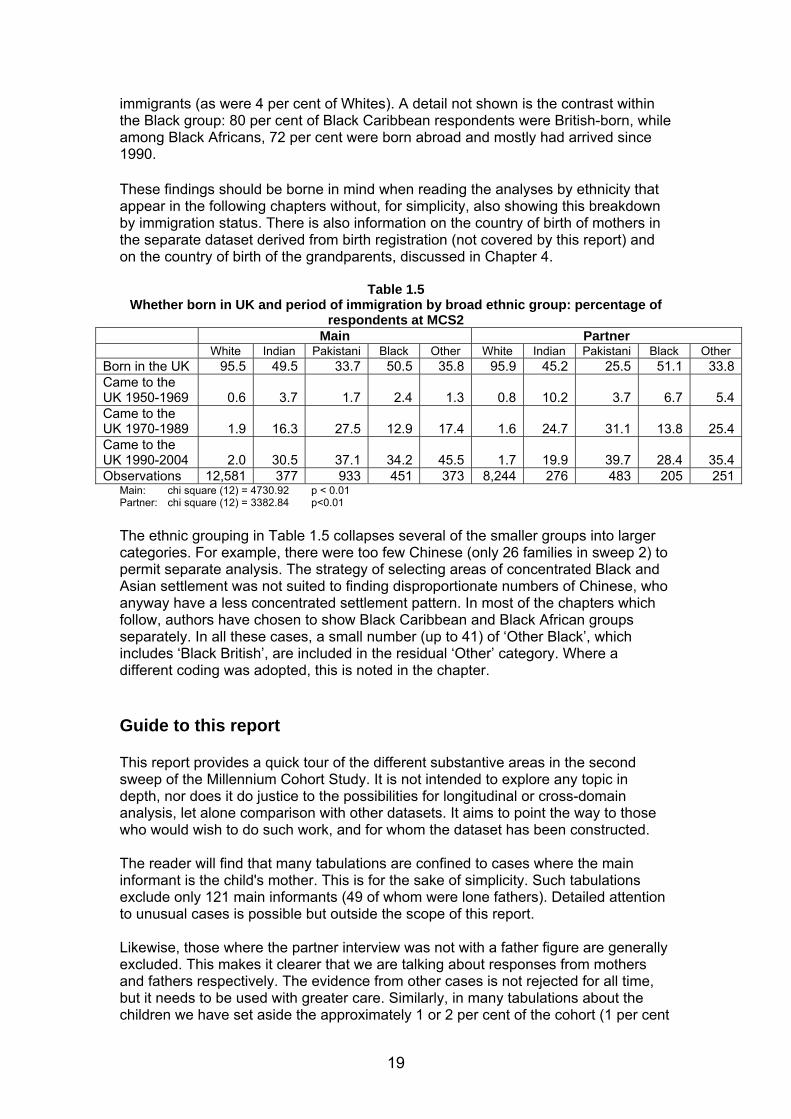
immigrants (as were 4 per cent of Whites). A detail not shown is the contrast within the Black group: 80 per cent of Black Caribbean respondents were British-born, while among Black Africans, 72 per cent were born abroad and mostly had arrived since 1990. These findings should be borne in mind when reading the analyses by ethnicity that appear in the following chapters without, for simplicity, also showing this breakdown by immigration status. There is also information on the country of birth of mothers in the separate dataset derived from birth registration (not covered by this report) and on the country of birth of the grandparents, discussed in Chapter 4.
Table 1.5 Whether born in UK and period of immigration by broad ethnic group: percentage of
respondents at MCS2 Main Partner White Indian Pakistani Black Other White Indian Pakistani Black Other
Born in the UK 95.5 49.5 33.7 50.5 35.8 95.9 45.2 25.5 51.1 33.8Came to the UK 1950-1969 0.6 3.7 1.7 2.4 1.3 0.8 10.2 3.7 6.7 5.4Came to the UK 1970-1989 1.9 16.3 27.5 12.9 17.4 1.6 24.7 31.1 13.8 25.4Came to the UK 1990-2004 2.0 30.5 37.1 34.2 45.5 1.7 19.9 39.7 28.4 35.4Observations 12,581 377 933 451 373 8,244 276 483 205 251
Main: chi square (12) = 4730.92 p < 0.01 Partner: chi square (12) = 3382.84 p<0.01 The ethnic grouping in Table 1.5 collapses several of the smaller groups into larger categories. For example, there were too few Chinese (only 26 families in sweep 2) to permit separate analysis. The strategy of selecting areas of concentrated Black and Asian settlement was not suited to finding disproportionate numbers of Chinese, who anyway have a less concentrated settlement pattern. In most of the chapters which follow, authors have chosen to show Black Caribbean and Black African groups separately. In all these cases, a small number (up to 41) of ‘Other Black’, which includes ‘Black British’, are included in the residual ‘Other’ category. Where a different coding was adopted, this is noted in the chapter. Guide to this report This report provides a quick tour of the different substantive areas in the second sweep of the Millennium Cohort Study. It is not intended to explore any topic in depth, nor does it do justice to the possibilities for longitudinal or cross-domain analysis, let alone comparison with other datasets. It aims to point the way to those who would wish to do such work, and for whom the dataset has been constructed. The reader will find that many tabulations are confined to cases where the main informant is the child's mother. This is for the sake of simplicity. Such tabulations exclude only 121 main informants (49 of whom were lone fathers). Detailed attention to unusual cases is possible but outside the scope of this report. Likewise, those where the partner interview was not with a father figure are generally excluded. This makes it clearer that we are talking about responses from mothers and fathers respectively. The evidence from other cases is not rejected for all time, but it needs to be used with greater care. Similarly, in many tabulations about the children we have set aside the approximately 1 or 2 per cent of the cohort (1 per cent
19

of families) where the children are twins or triplets, leaving the possibility for future analysis of these special cases. For some analyses requiring the fathers to have provided data, we do not include those two-parent families where the resident father did not complete an interview. The results here are generally presented as percentages weighted to correct for the different sampling probabilities of nine types of location at the first survey: two disadvantaged and ‘non-disadvantaged’ in each of the four countries, plus one covering wards in England with a high concentration of minority ethnic populations. The base numbers presented with these percentages are usually unweighted, which gives a better idea of the size of the underlying sample to potential future analysts, but which does not necessarily give a good idea of the size of sub-populations relative to each other. For example, the unweighted sample numbers for minority ethnic groups such as Bangladeshis tend to overstate their prevalence in the population since they are disproportionately recruited from types of ward that are over-sampled. We also allow for the survey design’s weighting and clustering in the tests of statistical significance that are reported. These use procedures available in the STATA analysis package. Findings selected for the Executive Summary and the Executive Briefings accompanying this report have been selected for statistical significance unless otherwise stated. We do not attempt to re-weight results for differential non-response or attrition. Note also that behind the averages and proportions lie the individual differences between every child. To say, for example, that girls are ahead of boys for a particular indicator such as vocabulary, on average, does not mean that all girls are ahead of all boys. It would also be quite wrong to suggest that all children from a particular disadvantaged background are destined to certain failure. The survey is setting out to chart the risks that threaten to limit the achievements of a new generation. Plan of the chapters Chapter 2 examines the housing, neighbourhood and community in which the cohort children are growing up. Chapters 3, 4 and 5 look at various aspects of the children’s families. Child health is surveyed in Chapter 6 and the children’s cognitive and behavioural development is the focus of Chapter 7. Chapters 8, 9 and 10 look in more detail at the children’s parents: their health and lifestyle in Chapter 8; their education and employment in Chapter 9; and their income in Chapter 10. Childcare is examined in Chapter 11, while older siblings make an appearance in Chapter 12. References Dex, S. and Joshi, H. (eds) (2005) Children of the 21st Century: from Birth to 9 months, Bristol: Policy Press Hansen, K. (ed) (2006) Millennium Cohort Study First and Second Surveys; Guide to the Dataset. First Edition, London: Centre for Longitudinal Studies, Institute of Education. http://www.cls.ioe.ac.uk/studies.asp?section=00010002000100040008
20

MCS Team (2006) MCS Derived variables, London: Centre for Longitudinal Studies, Institute of Education. http://www.cls.ioe.ac.uk/studies.asp?section=00010002000100040007 Moon, N. (2006) Technical Report on Fieldwork, London: NOP. http://www.cls.ioe.ac.uk/studies.asp?section=00010002000100040006Plewis, I. (ed) (2004) Millennium Cohort Study First Survey: Technical Report on Sampling (3rd Edition). London: Centre for Longitudinal Studies, Institute of Education. http://www.cls.ioe.ac.uk/studies.asp?section=0001000200010010 Plewis, I. and Ketende, S. (2006) Millennium Cohort Study: Technical Report on Response (first edition). London: Centre for Longitudinal Studies, Institute of Education. http://www.cls.ioe.ac.uk/studies.asp?section=00010002000100040006
21

Chapter 2 HOUSING, NEIGHBOURHOOD AND COMMUNITY Gareth Hughes, Sosthenes Ketende and Ian Plewis Introduction This chapter embellishes the results from MCS1 by focusing on changes between it and MCS2 in terms of house-moving and families’ perception of their area. Families can move home for many reasons, including dissatisfaction with accommodation or the neighbourhood, a change of employment, or the wish to be closer to (or further away from) other family members. Often, mobility will benefit both parents and children, but it can also result in a loss of contact with services and the disappearance of a supportive network of neighbours. Travel may also become more difficult. Here we look at some socio-economic and socio-demographic correlates of mobility. Mobility In this section, we look at characteristics of mobile families at sweep 2 and their reason(s) for moving home. MCS1 took place when the cohort children were about nine months old and the second sweep when they were about three years old and so we are looking at residential mobility for the intervening period. The base for Tables 2.1 to 2.7 is all families who were productive at MCS1 and eligible for sweep 2 (as explained in Chapter 1, a family’s response is considered ‘productive’ if there are data from any one of six instruments used at sweep 2). This definition excludes the ‘new families’. Thirty-eight per cent of families changed address between sweeps 1 and 2 (Table 2.1). These figures are based on information from the administrative address database at CLS. There were country differences: Scotland had the highest proportion of families who moved (41 per cent) and Northern Ireland the lowest (33 per cent).
Table 2.1 Mobility by UK country
UK country at sweep 1 Mobile
% (n)
Base (n)
England 38.1 (4,432) 11,426Wales 34.8 (996) 2,744Scotland 40.6 (964) 2,303Northern Ireland 32.6 (640) 1,912Total 38.0 (7,032) 18,385Note: Weighted percentages; observed sample numbers. Chi square: 17, P value: 0.0041
22

Indian, Pakistani and Bangladeshi families were less mobile than the other ethnic groups (Table 2.2).
Table 2.2 Residential mobility by ethnic group of the main respondent between sweeps 1 and 2
Main respondent’s ethnic group Mobile
% (n)
Base (n)
White 38 (5,992) 15,398Mixed 42 (81) 186Indian 31 (150) 479Pakistani 31 (278) 891Bangladeshi 33 (118) 370Black Caribbean 37 (94) 262Black African 37 (145) 378Other (inc. Chinese, other Asian, other Black) 43 (156) 374Total 38 (7,014) 18,338Note: Weighted percentages; observed sample numbers
Chi square: 24, P value: 0.0017 Families in houses or bungalows were less likely to move than those in other types of accommodation (Table 2.3). Likewise, homeowners were less likely to move than tenants (Table 2.4).
Table 2.3 Residential mobility by type of accommodation at sweep 1
Type of accommodation Mobile % (n)
Base (n)
House or bungalow 34.7 (5,428) 15,587 Flat or maisonette 58.8 (1,506) 2,650 Other (studio flat, rooms, bedsit, etc) 73.5 (78) 104 Total 37.9 (7,012) 18,341 Note: Weighted percentages; observed sample numbers
Chi square: 23, P value: 0.0012
Table 2.4 Residential mobility by tenure at sweep 1
Housing tenure Mobile % (n)
Base (n)
Buying 30.9 (3,236) 10,603Renting 47.9 (3,076) 6,558Other* 63.1 (694) 1,166Total 37.9 (7,006) 18,327Note: Weighted percentages; observed sample numbers
*Other includes living with parents, living rent-free, squatting. Chi square: 759, P value: <0.001
Lower-income families were more likely to change addresses between the two sweeps than high-income families (Table 2.5). Income and tenure are closely related. Of the families who were renting at sweep 2, 46 per cent were recipients of the means-tested Housing Benefit.
23

Table 2.5 Residential mobility by family income at sweep 1
Family income (banded)
Mobile % (n)
Base (n)
£0 - £10,400 pa 48.5 (2,226) 4,701£10,400 - £20,800 pa 36.7 (1,981) 5,590£20,800 - £31,200 pa 33.6 (1,121) 3,275£31,200 - £52,000 pa 34.2 (826) 2,377£52,000-plus pa 37.7 (322) 847Don't know 34.6 (376) 1,083Refused to answer 34.8 (166) 476Total 37.9 (7,018) 18,349
Note: Weighted percentages; observed sample numbers Chi square: 237: P value: <0.001
About half the renters are local authority tenants, a quarter rent from housing associations and the remainder rent privately. More than half of the renters (53 per cent at sweep1) received state benefit for their accommodation through Housing Benefit or Income Support. Very few of the owner-occupiers (1.5 per cent) did so. A quarter of the movers had been receiving one or other benefit (or both), compared to one-sixth (15.6 percent) of the families who did not move (table not shown). Of those families interviewed at sweep 2, the predominance of means-tested benefits for renters continued. One-third of renters (34.6 per cent) reported receiving both Housing Benefit and Income Support, 11.4 per cent Housing Benefit only and 7 per cent Income Support only, which leaves 47.1 per cent reporting no cash help, in contrast to 98.6 per cent of home-owners and 80.6 per cent of the small group in other housing arrangements. Families where both the main respondent and partner or only the partner was in paid work were less likely to move than families with no earner or where only the main respondent (mostly the mother) was in paid work (Table 2.6).
Table 2.6 Residential mobility by combined labour market status of main and partner
respondents at sweep 1
Paid work status of the cohort families at sweep 1Mobile
% (n)
Base (n)
Both in work/on leave 33.3 (2,536) 7,504Main in work/on leave, partner not in work/on leave 43.5 (176) 424Partner in work/on leave, main not in work/on leave 37.2 (2,069) 5,754Both not in work/on leave 44.8 (658) 1,513Total 35.9 (5,439) 15,195Note: Weighted percentages; observed sample numbers
Single parents are excluded Chi square: 75, P value: <0.001
Table 2.7 shows that families in Scotland moved the longest distance on average (35 kilometres) whereas families in Northern Ireland moved the shortest distance (11 kilometres).
24

Table 2.7 Distance moved between sweeps 1 and 2 by UK country
Distance in kilometres UK country at sweep 1 Mean Standard error 95 per cent CI England 24.6 1.6 21.4 - 27.8Wales 12.6 1.3 10.1 - 15.1Scotland 35.1 6.0 23.3 - 46.9Northern Ireland 10.8 1.7 7.4 - 14.2
Note: Movements both within and between UK countries but excluding international migrants who were ineligible for sweep 2.
Table 2.8
Distance moved between the two sweeps UK country at sweep 1 Distance moved
(km)
England %
Wales %
Scotland %
Northern Ireland %
0<1 29 40 37 331<2 22 18 16 203<11 20 20 19 2011+ 19 12 20 18Unknown 9.2 9.5 9 9.2Base (n) 4,432 996 964 640Note: Distances are straight lines between the centres of postcode areas Chi square: 50, p<0.001 Table 2.8 shows that less than one-fifth of families moved more than 10 kilometres. About 9 per cent of families did not report a move that was recorded in the tracing data. The proportion of families living in a house or bungalow increased from 81 per cent to 89 per cent between sweeps 1 and 2 for those movers interviewed at sweep 2. There was also an increase from 56 per cent to 59 per cent in the number of families buying their home. The proportion of movers ’very satisfied’ with their home increased from 30 per cent at sweep 1 to 44 per cent at sweep 2 for the movers and those ‘very dissatisfied’ with their home decreased from 6 per cent at sweep 1 to 2 per cent at sweep 2. The most popular reason for moving given by those interviewed at sweep 2 was wanting a larger home. This was followed by wanting to move to a better area (Table 2.9).
Table 2.9 MCS2 distribution of reasons for moving
What were the main reasons you moved to this address? Per cent (n)
Base
Wanted larger home 47.2 (1,960)Wanted to move to better area 22.7 (988)Wanted better home 20.7 (893)To be nearer relative(s) 12.3 (508)For children's education 12.3 (504)Wanted place of my own 10 (523)Relationship breakdown 7.5 (354) 4,428Wanted to buy 6.3 (292)Job change/nearer work 6.2 (229)Problem with neighbours 4.9 (241)Spouse or partner job change 3.5 (138)
25

Table 2.9
What were the main reasons you moved to this address? Per cent (n)
MCS2 distribution of reasons for moving
Base Contd.. Just wanted a change 3.7 (151)New relationship 1.7 (75)Evicted/repossessed 1.6 (74)Could no longer afford home 1.6 (71)Note: Weighted percentages; observed sample numbers.
Respondents could give more than one response. Based on movers who were productive at sweep 2.
Area There was little change in satisfaction with the area for those families who did not move between sweeps 1 and 2: 73 per cent of those ‘very satisfied’ at sweep 1 remained so at sweep 2. For those families who moved, however, 53 per cent were very satisfied at sweep 2, compared with just 36 per cent at sweep 1.
Table 2.10 UK country of interview at sweep 2, by ‘Good area to bring up children’
UK country at sweep 1 England Wales Scotland N Ireland Total
Excellent 32.3 35.3 41.3 45.5 33.7Good 40.1 39.9 37.0 38.4 39.7Average 19.4 18.1 16.2 11.7 18.8Poor 5.1 4.3 3.4 2.8 4.8Very poor 3.1 2.4 2.1 1.6 2.9
‘Good area to bring up children’
Total 100.0
(9,264)100.0
(2,219)100.0
(1,792)100.0
(1,445) 100.0
(14,720)Note: Weighted percentages; observed sample numbers.
Chi square: 75.7, P value: <0.001
Table 2.11 UK country of interview by ‘How safe you feel in area’
UK country at sweep 2 England Wales Scotland N Ireland Total
Very safe 37.0 43.8 41.7 51.8 40.3Fairly safe 50.6 46.1 49.2 42.8 48.9Neither safe nor unsafe 6.5 5.5 5.4 2.4 5.7Fairly unsafe 4.2 3.4 2.7 2.1 3.7Very unsafe 1.6 1.3 1.0 0.9 1.4
‘How safe you feel in area’
Total 100.0
(9,302)100.0
(2,222)100.0
(1,795)100.0
(1,445) 100.0
(14,764)Note: Weighted percentages; observed sample numbers.
Chi square: 165.4, P value: <0.001
Few respondents reported their areas as poor, or very poor places to bring up children (7 per cent), or fairly or very unsafe (6 per cent). Northern Ireland seems to be perceived as the ‘best’ area to bring up children and the safest overall.
26

Table 2.12 Cohort child’s ethnic group by ‘Good area to bring up children’ (weighted proportions)
Cohort child’s ethnic group
White Indian Pakistani Bangladeshi Black Mixed & other Total
Excellent 35.2 31.9 23.8 11.9 13.9 21.5 33.7Good 39.3 43.5 41.4 43.2 45.6 43.4 39.8Average 18.3 18.1 22.1 29.7 25.2 22.9 18.8Poor 4.5 4.2 8.5 11.0 8.1 6.6 4.8Very poor 2.7 2.3 4.3 4.2 7.1 5.6 2.9
MCS2 ‘Good area to bring up children’
Total 100.0
(12,351) 100.0(362)
100.0(671)
100.0(257)
100.0 (432)
100.0(628)
100.0(14,701)
Note: Weighted percentages; observed sample numbers. Chi square: 165.2, P value: <0.001
Table 2.13
Cohort child’s ethnic group by ‘How safe you feel in area’ Cohort child’s ethnic group
White Indian Pakistani Bangladeshi Black Mixed and other Total
Very safe 38.6 35.1 39.6 35.6 30.1 31.3 38.1
Fairly safe 50.4 50.8 45.3 48.3 48.4 49.7 50.2Neither safe nor unsafe 5.9 9.2 6.4 6.8 8.7 9.0 6.2Fairly unsafe 3.7 3.8 5.4 6.8 9.3 6.5 4.0Very unsafe 1.4 1.1 3.2 2.5 3.5 3.5 1.5
MCS2 ‘How safe you feel in area’
Total 100.0
12,373 100.0(366)
100.0(678)
100.0(258)
100.0 (438)
100.0(632)
100.0(14,745)
Note: Weighted percentages; observed sample numbers. Chi square: 87.7, P value: <0.001
Families with White and Indian children are more likely to perceive their area as being excellent for bringing up children. Families of Black children are most likely to think their area is ‘very poor’, and least likely to think it is ‘very safe’.
Table 2.14
Main respondent’s NS-SEC (five-fold classification) by ‘Good area to bring up children’ NS-SEC five classes at MCS1 interview (main respondent)
Management and professional Intermediate
Small employer and self-employed
Low supervisory and technical
Semi-routine and routine Total
Excellent 45.0 34.6 46.0 31.2 23.5 34.8Good 40.1 43.3 36.7 35.0 38.5 39.7Average 11.8 16.8 13.8 22.7 26.0 18.3Poor 2.3 3.7 2.5 6.7 7.1 4.5Very poor 0.8 1.7 1.1 4.4 4.9 2.6
MCS2 ‘Good area to bring up children’
Total 100.0
(4,187) 100.0
(2,551)100.0(530)
100.0 (806)
100.0(5,156)
100.0(13,230)
Note: Weighted percentages; observed sample numbers. Only includes those who were working (or on leave) at the time of interview (MCS1). Chi square: 887.0, P value: <0.001
27

Table 2.15 Main respondent’s NS-SEC (five-fold classification) by ‘How safe you feel in area’
NS-SEC five classes at MCS1 interview (main respondent)
Management & professional Intermediate
Small employer & self-employed
Low supply & technical
Semi-routine & routine Total
Very safe 44.9 39.4 41.8 35.3 32.0 38.7Fairly safe 49.0 50.9 51.5 50.4 51.3 50.3Neither safe nor unsafe 3.9 5.8 4.9 7.5 8.0 5.9Fairly unsafe 2.0 3.0 1.1 4.8 6.1 3.7Very unsafe 0.3 0.9 0.8 2.0 2.6 1.3
MCS2 ‘How
safe you feel in area’
Total 100.0
(4,187) 100.0
(2,551)100.0(530)
100.0 (806)
100.0(5,156)
100.0(13,230)
Note: Weighted percentages; observed sample numbers. Only includes those who were working (or on leave) at the time of interview (MCS1). Chi square: 378.4, P value: <0.001
There is a general trend among those in a higher NS-SEC group to perceive their area as being ‘excellent’ for bringing up children and ‘very safe’. ‘Semi-routine and routine’ have the highest proportion of those believing their area is ‘average’ or worse for bringing up children, but even for mothers in the least advantaged occupational class, only a minority reported their areas as poor/very poor (12 per cent) or fairly/very unsafe (9 per cent). Home atmosphere Three variables, each with five ordered categories, relate to the atmosphere of the home (‘disorganised’, ‘hearing yourself think’ and ‘calm’). These variables are correlated – the values of Kendall’s tau vary between 0.33 and 0.41 – and so they can be added together to form a scale measuring ‘home activity’ or ‘home atmosphere’ between zero (‘hectic’) and 12 (‘calm’). This scale is skewed towards the calm end with a median of eight, with 11 per cent scoring 11 or 12 but less than 1 per cent scoring below two. Table 2.15 gives the means by UK country, minority ethnic group, parents’ labour market status and the number of parents/carers in the household. It shows that homes in Northern Ireland are the most calm, and homes in Wales the least calm (p < 0.01); that minority ethnic main respondents, notably those from an Indian background, live in homes that are reported to be calmer than White homes (p < 0.001); that where both parents are in work, the home is said to be calmer than if neither is working (p < 0.001); and where there are two parents the home is rated somewhat calmer (p < 0.001).
28

Table 2.15 Home activity (weighted means) by UK country at sweep 2,
ethnic group, parents’ labour market status and number of parents Mean Standard
error 95 per cent CI
England 8.0 0.048 7.9 – 8.1Wales 7.9 0.052 7.8 - 8.0Scotland 7.9 0.064 7.8 – 8.1
UK country at sweep 2 (n = 15,446)
Northern Ireland 8.2 0.078 8.1 – 8.4White 7.9 0.037 7.9 – 8.0Mixed 8.1 0.21 7.7 – 8.6Indian 9.3 0.25 8.8 – 9.8Pakistani and Bangladeshi
8.5 0.11 8.3 – 8.7
Black 8.5 0.13 8.3 – 8.8
Ethnic group of main respondent (n = 14,714)
Other 8.8 0.15 8.5 – 9.1Both in work 8.2 0.047 8.1 – 8.3Only main in work 7.7 0.15 7.4 – 8.0Only partner in work 7.9 0.051 7.8 – 8.0
Parental work status (n = 12,733)
Neither in work 7.1 0.12 6.9 – 7.4One 7.8 0.067 7.7 – 7.9Parents in home
(n = 15,446) Two 8.0 0.043 8.0 – 8.1Note: Observed sample numbers. Conclusion Residential mobility is an important feature of the lives of families with young children: more than one-third of the sample from sweep 1 had changed address in the intervening 27 or so months. Most families do not move very far, however, and many stay in the same neighbourhood. This mobility is socially and geographically patterned; being more common in Scotland than in Northern Ireland; less common in families with a South Asian background; and more common in the lower income, flat-dwelling and renting groups at sweep1. When compared with the other UK countries, the main respondents in Northern Ireland have a more positive view about their area in terms of bringing up children and feeling safe. They also report a calmer home atmosphere. These findings – and the links between them – warrant further investigation. It would also then be possible to compare the main respondents’ and the interviewers’ perceptions of the same local area.
29

Chapter 3 FAMILY DEMOGRAPHICS Lisa Calderwood Introduction This chapter is concerned with the cohort child’s parents and the immediate family with whom he or she shares a home. Whether they live with one or two parents will not only make many differences to the child’s experience of growing up, it will also affect whether the study is able to gather the father’s perspective as well as the mother’s on several questions in the survey. The number of adults contributing to the household income will also affect the outcome for the child. This chapter looks at the number of parents in the home, whether and how this has changed since the first survey, whether two-parent families are headed by married couples, and changes in that marital status. It then turns to siblings and grandparents living in the same household. The chapter ends with a look beyond the child’s home at parents who are not resident, mostly fathers, and their relationship with the cohort child. The economic and emotional ties of those children with parents outside the home have become an important feature of family life. The key measure of family demographics included in the survey is the household grid. This collects (from the main respondent at the beginning of the interview) the individual details (name, sex and date of birth) of all adults and children in the cohort child’s household. The main respondent was asked to include ‘people who live here regularly as members of this household’. It also collects a complete set of relationships between everyone in the household. Most of the findings in this chapter use only information collected in the household grid. The exception is the information about the cohort child’s relationship with their non-resident father, which is taken from the interview with the main respondent. Family type, parents and partnerships Family type Most children were living with both of their natural parents at age three, though this proportion had fallen slightly from 85.8 per cent of the sample interviewed at nine months to 82 per cent of the cross-section in the second survey (Table 3.1). Typically, the child’s natural parents were also married to each other. This arrangement accounted for around six in 10 families at both sweeps. The proportion of families in which the natural parents were living together without being married fell from 24 per cent at sweep 1 to 14.8 per cent at sweep 2. However, much of this difference is due to a big increase in the proportion of families in which the relationship between natural parents was ‘other’ (neither married nor cohabiting) or was ‘unknown’ (don’t know, refused to answer or missing data); from 0.4 per cent to 4.3 per cent.
30

If children were not living with both natural parents, they were usually in lone-parent families with their natural mother. The proportion of children in lone natural-mother families increased slightly from 13.7 per cent at nine months to 14.9 per cent at three years. A small proportion of children were living in ‘other’ family types, though the prevalence of such families had increased from 0.5 per cent at nine months to 3.1 per cent at three years. Most of these ‘other’ family types at age three were a natural mother and another parent/partner (2.2 per cent). There were very few lone natural fathers (0.4 per cent), natural fathers living with another parent/partner (0.1 per cent), adoptive parents (0.1 per cent) and grandparents (0.2 per cent). The remainder (0.1 per cent) were other or unknown family types.
Table 3.1
Family type by country Country at MCS1 Country at MCS2 Family type England Wales Scotland Northern
Ireland UK England Wales Scotland Northern Ireland UK
% % % % % % % % % % Both natural parents 86.2 81.8 85.3 83.2 85.8 81.7 80.6 84.4 84.1 82.0Married 61.6 57.1 59.9 68.3 61.4 62.7 58.6 63.7 71.6 62.9Cohabiting 24.3 24.3 24.8 14.0 24.0 14.7 16.8 17.0 8.5 14.8Other/unknown relationship 0.4 0.5 0.6 0.9 0.4 4.3 5.2 3.7 4.0 4.3Lone natural mother 13.3 17.6 14.3 16.7 13.7 15.1 16.3 12.8 14.7 14.9Other family type 0.5 0.6 0.4 0.1 0.5 3.2 3.1 2.8 1.2 3.1Base (weighted) 9,880 2,726 2,302 1,931 18,392 8,841 2,218 1,789 1,480 16,027Base (unweighted) 11,533 2,760 2,336 1,923 18,552 10,107 2,233 1,800 1,450 15,590
MCS1 Chi square: 171.94, p=0.0000 MCS2 Chi square: 118.29, p=0.0000 Base: All families interviewed at MCS1 Base: All families interviewed at MCS2
Table 3.2
Family type by mother’s age at MCS2 interview
Family type 16-24 25-29 30-34 35-39 40+ Total % % % % % % Both natural parents 49.7 76.8 88.7 90.9 90.2 82.8Married 20.6 51.9 72.5 76.8 72.8 64.0Cohabiting 26.2 20.8 12.5 10.4 13.7 15.1Other/unknown relationship 2.9 4.2 3.7 3.7 3.7 3.7Lone natural mother 42.5 19.9 9.8 8.1 8.6 14.8Other family type 7.8 3.3 1.5 1.1 1.1 2.4Base (weighted) 1,864 2,741 5,161 4,399 1,536 15,701
Chi square: 2595.79, p=0.0000 Base (unweighted) 2,155 3,000 4,830 3,877 1,373 15,235
Base: All families in which the main respondent was a mother (any type of mother) and in which mother’s age was known.
31

Table 3.3 Family type by child’s ethnic group
Family type White Mixed Indian Pakistani Bangla- deshi
Black Caribbean
Black African
Other ethnic group
Total
% % % % % % % % % Both natural parents 82.8 67.3 93.9 90.2 91.9 53.1 66.0 79.9 82.3Married 62.9 48.1 85.2 81.3 79.6 31.8 56.5 63.3 63.2Cohabiting 15.9 14.4 0.3 1.0 2.3 16.7 6.4 6.6 14.9Other/unknown relationship 4.0 4.8 8.5 7.9 10.1 4.6 3.0 10.0 4.3Lone natural mother 14.3 30.2 5.0 8.5 6.7 46.6 31.6 18.0 14.9Other family type 2.9 2.5 1.1 1.2 1.3 0.3 2.4 2.0 2.7Base (weighted) 14,070 472 284 440 129 132 204 189 15,920
Chi square: 524.76, p=0.0000 Base (unweighted) 12,894 449 401 734 282 180 289 260 15,489
Base: All families in which the cohort child’s ethnic group was known. Wales had the highest proportion of lone natural-mother families in the cross-sections at both sweeps and Northern Ireland had the highest proportion of married natural-parent families at both sweeps. Interestingly, in Wales, Scotland and Northern Ireland there was actually a lower proportion of lone natural-mother families at age three than at nine months, though in England the proportion had increased. Lone parenthood was more common among younger mothers; 42.5 per cent of mothers aged 16 to 24 and 19.9 per cent of mothers aged 25 to 29 were lone parents. Younger mothers were also less likely to be married and living with the child’s father: a fifth (20.6 per cent of mothers aged 16 to 24) were in this situation. Indian, Pakistani and Bangladeshi children were the most likely to be living with both natural parents (more than 90 per cent) and their parents were almost always married to each other. Living with cohabitating parents was extremely rare for children in these ethnic groups. In contrast, lone parenthood was a relatively common experience for children in some other ethnic groups. Nearly half (46.6 per cent) of Black Caribbean children and a third of Mixed and Black African children (30.2 per cent and 31.6 per cent respectively) were living with a lone natural mother. Change in family type For those families who took part in both sweep 1 and sweep 2, the composition of the household at each sweep can be compared longitudinally to examine changes in family type. A broad definition of ‘parents’ is used which includes step-parents and partners of parents as well as ‘parent-figures’ such as grandparents. For instance, a child living with both grandparents (and no parents) at both sweeps would be treated as remaining in the same two-parent family for this analysis. However, as reported earlier, these ‘other’ family types account for a very small proportion of families. Overall, 93.1 per cent of two-parent families at sweep 1 were still two-parent families at sweep 2 and 27.9 per cent of one-parent families at sweep 1 had acquired a second parent by sweep 2 (Table 3.4). Of all the families interviewed for both surveys, parents had parted company in 6 per cent of cases and 3 per cent were single parents the first time around who had
32

gained a second parent. The proportion of families in this sample in Table 3.4 who were lone parents went up from 12 per cent to 15 per cent. Note that there was differential loss from the survey of lone-parent families from the first survey, which can be inferred from a comparison of Tables 3.4 and 3.1 where a higher proportion of lone mothers is apparent in the cross-sectional sample for sweep1. There were some small differences between countries in the proportion of two-parent families from sweep 1 who were still two-parent families at sweep 2 but these were not statistically significant. However, there was significant country variation in the proportion of one-parent families from sweep 1 which had become two-parent families at sweep 2. One-parent families in Scotland and Northern Ireland were the most likely to acquire another parent by sweep 2 (35.9 per cent and 31.3 per cent respectively) and one-parent families in England were the least likely to acquire another parent by sweep 2 (26.7 per cent).
Table 3.4
Change in family type by country
Country at MCS2 Family type at MCS1
Family type at MCS2
England Wales Scotland Northern Ireland
UK
% % % % % Two-parent family 92.8 93.3 94.3 94.7 93.1
Two-parent family
One-parent family 7.2 6.7 5.7 5.3 6.9
Base (weighted) 7,242 1,843 1,544 1,249 13,201Base (unweighted) 7,956 1,770 1,527 1,180 12,433
Two-parent family 26.7 29.5 35.9 31.3 27.9
One-parent family
One-parent family 73.3 70.5 64.1 68.7 72.1
Base (weighted) 949 345 224 227 1811
Two-parent family at MCS1 Chi square: 9.73, p=0.0630 Base (unweighted) 1,307 428 250 264 2,249
One-parent family at MCS1 Chi square: 10.60, p=0.0269 Base: All families who took part in both MCS1 and MCS2 and were in either a two-parent family or a one-parent family at both MCS1 and MCS2. Most of the second parents acquired by sweep 2 by one-parent families at sweep 1 were the cohort child’s natural father (about 71 per cent1). In slightly under a quarter of families (23 per cent), this additional parent was a stepfather. Change in family type showed some interesting variation with the mother’s age (Table 3.5). Mothers aged between 16 and 24 at the MCS2 interview who were in two-parent families at sweep 1 were significantly less likely (77.5 per cent) to be still in those two-parent families at sweep 2 than older mothers (at least 95 per cent of those aged 30 and over). Mothers aged 25 to 29 occupied an intermediate position closer to the older age-groups (at 89.4 per cent). However, younger mothers who were lone parents at sweep 1 were also more likely to have acquired a second partner at sweep 2. Mothers aged 25 to 29 were most likely to have experienced this change (32.5 per cent), followed by those aged 16 to 24 (29.6 per cent). About a quarter of those aged 30 to 34 and 40 and over had 1 In 5 per cent of families the new parent was a natural parent but their sex was not known. Here they are assumed to be male and included in this proportion.
33

acquired a second parent for their children and the group aged 35 to 39 were the least likely to have done so (22.1 per cent).
Table 3.5 Change in family type by mother’s age at MCS2 interview
Family type at MCS1
Family type at MCS2
16-24 25-29 30-34 35-39 40+ Total
% % % % % % Two-parent family Two-parent
family 77.5 89.4 95.6 96.6 96.6 93.7 One-parent
family 22.5 10.6 4.4 3.4 3.4 6.3Base (weighted) 948 2,142 4,594 3,936 1,353 12,972Base (unweighted) 1,070 2,282 4,230 3,415 1,188 12,185
Two-parent family 29.6 32.4 25.7 22.1 24.7
Two-parent family at MCS1 Chi square: 552.52, p=0.0000 One-parent family at MCS1 Chi square: 13.30, p=0.0390 Base: All families who took part in both MCS1 and MCS2 and were in either a two-parent family or a one-parent family at both MCS1 and MCS2 and in which the main respondent at MCS2 was a mother (any type of mother) for whom age was known. Transition from cohabitation to marriage For those families who took part in both sweep 1 and sweep 2, the relationships between family members can be compared longitudinally. This section looks at transitions from cohabitation to marriage in families in which the child was living with both natural parents at sweep 1 and sweep 2 and where the parents were living together without being married at sweep 1. Almost a third (29.7 per cent) of those parents who were cohabiting at sweep 1 were married to each other by sweep 2 (Table 3.6). This varied considerably by country, with cohabiting parents in Northern Ireland most likely to get married (44.8 per cent), followed by England (30.2 per cent), Wales (27.0 per cent) and Scotland (24.4 per cent).
Table 3.6 Transition from cohabitation to marriage by country
Chi square: 23.69, p=0.0001 Base: All families who took part in both MCS1 and MCS2, who were in a family with cohabiting natural parents at MCS2 and were in a family in which the same two parents were still present at MCS2 and the relationship between the parents at MCS2 was known. This also varied significantly by the mother’s age, with the youngest and oldest age-groups least likely to get married. Looking at mothers who were cohabiting at sweep
28.2One-parent family
One-parent family 70.4 67.6 74.3 77.9 75.3 71.8
Base (weighted) 668 409 351 250 101 1,780Base (unweighted) 858 532 411 293 124 2,218
Country at MCS2 Family type at MCS1
Family type at MCS2
England Wales Scotland Northern Ireland
UK
% % % % % Married natural parents 30.2 27.0 24.4 44.8 29.7
Cohabiting natural parents
Cohabiting natural parents 69.8 73.0 75.6 55.2 70.3
Base (weighted) 1,573 432 337 145 2,845Base (unweighted) 1,687 472 355 154 2,668
34

1,22.7 per cent of the 16 to 24 age group and 22.5 per cent of the 40 and over age group had got married compared with around 30 to 34 per cent in the other age groups.
Table 3.7 Transition from cohabitation to marriage by mother’s age at MCS2 interview
Family type at MCS1
Family type at MCS2
16-24 25-29 30-34 35-39 40+ Total
% % % % % % Cohabiting natural parents
Married natural parents 22.7 34.0 30.1 32.4 22.5 29.7
Cohabiting natural parents 77.3 66.0 69.9 67.6 77.5 70.3
Base (weighted) 469 710 826 592 242 2,838
Chi square=23.86, p=0.0044 Base (unweighted) 517 700 740 504 201 2,662
Base: All families who took part in both MCS1 and MCS2, who were in a family with cohabiting natural parents at MCS2 and were in a family in which the same two parents were still present at MCS2 and the relationship between the parents at MCS2 was known and where the main respondent was a mother (any type of mother) for whom age was known. Siblings In this section, the relationship to the cohort child collected in the household grid is used to identify which of the other children (and adults) in the household were the natural, step, foster, adoptive or half-siblings of the cohort child. The dates of birth of these siblings are also used to identify both older and younger siblings of the cohort child. The definition of siblings in this context excludes siblings from multiple births who are also cohort children. Hence in a family with twin cohort children and no other siblings, the cohort children would be classified as having no siblings in this analysis. Number of siblings At age three, a quarter of children had no brothers or sisters (in the same household) compared with more than four in 10 (42.8 per cent) at nine months. The majority of those with siblings – 47.7 per cent of all children – had just one brother or sister and fewer than one in 10 (8.8 per cent) had three or more siblings (Table 3.8). The number of siblings per household varied by country, mother’s age and child’s ethnic group. Children in Northern Ireland were the least likely still to have no siblings (22.5 per cent) and the most likely to have three or more brothers and sisters (14.2 per cent) at age three. Children in Scotland were the least likely to have three or more siblings (6.2 per cent).
35

Table 3.8 Number of siblings in household at MCS1 and MCS2 by country
Country at MCS1 Country at MCS2 Siblings in household England Wales Scotland Northern
Ireland UK England Wales Scotland Northern Ireland UK
% % % % % % % % % % None
42.7 42.5 45.3 39.1 42.8 24.9 27.7 26.3 22.5 25.0One
36.2 36.8 35.7 32.6 36 48.0 45.2 49.5 39.5 47.7Two
14.5 14.3 14.1 18.0 15 18.3 18.3 18.0 23.8 18.4Three or more
6.6 6.5 4.9 10.3 6.6 8.9 8.8 6.2 14.2 8.8Base (weighted) 9,880 2,726 2,302 1,931 18,392 8,747 2,208 1,785 1,474 15,894Base (unweighted) 11,533 2,760 2,336 1,923 18,552 9,987 2,222 1,795 1,444 15,448
MCS1 Chi square: 89.64, p=0.0000 MCS2 Chi2=125.43 p=0.0000 MCS1 Base: All families interviewed at MCS1. MCS2 Base: All families interviewed at MCS2 in which the main respondent was interviewed. Almost half (49.2 per cent) of children whose mothers were aged 16 to 24 did not have any brothers or sisters and a further 39.4 per cent had only one sibling. Only one in 10 children with mothers in this age group had two or more siblings, compared with about one in three children with mothers aged 35 to 39 and 40 and over (Table 3.9).
Table 3.9 Number of siblings in household by mother’s age at MCS2 interview
Siblings in household 16-24 25-29 30-34 35-39 40+ Total % % % % % % None 49.2 27.9 22.9 17.8 16.3 24.8One 39.4 48.1 50.9 49.7 42.6 47.9Two 9.2 17.0 17.9 21.5 25.8 18.5Three or more 2.3 6.9 8.3 11.0 15.2 8.8Base (weighted) 1,860 2,740 5,155 4,395 1,534 15,634Base (unweighted) 2,151 2,997 4,824 3,875 1,372
15,219
Ch square: 971.31, p=0.0000 Base: All families interviewed at MCS2 in which the main respondent was interviewed and in which the main respondent was a mother (any kind of mother) for whom age was known. Bangladeshi, Pakistani and Black African children were the most likely to have many brothers and sisters; 32.6 per cent, 23.9 per cent, and 22.8 per cent respectively had three or more siblings (Table 3.10). However, Indian children were the least likely to have three or more siblings (4.8 per cent), while Pakistani and Bangladeshi children were the least likely to have no brothers and sisters (14 per cent and 15.6 per cent respectively).
36

Table 3.10 Number of siblings in household by child’s ethnic group
Child’s ethnic group Siblings in household White Mixed Indian Pakistani Bangladeshi Black
Caribbean Black
African
Other ethnic group
Total
% % % % % % % % % None 25.2 32.7 24.9 14.0 15.6 26.8 21.5 23.0 25.0One 48.9 40.6 46.8 34.0 26.0 41.6 28.3 46.3 47.7Two 17.9 18.7 23.6 28.2 25.7 19.7 27.4 16.9 18.4Three or more 8.0 8.0 4.8 23.9 32.6 11.9 22.8 13.7 8.8Base (weighted) 13,975 468 283 436 128 132 199 189 15,810
Chi square:383.28, p=0.0000
Base (unweighted) 12,795 446 398 728 278 179 284 260 15,368
Base: All families interviewed at MCS2 in which the main respondent was interviewed and in which the cohort child’s ethnic group was known. Older and younger siblings Overall, 26.9 per cent of children had at least one younger sibling. Nearly 18 per cent had younger siblings only and 9.2 per cent had both older and younger siblings. A higher proportion of children (57.2 per cent) had an older sibling. Forty-eight per cent had older siblings only and 9.2 per cent had both older and younger siblings (Table 3.11). Children in Northern Ireland were the most likely to have both older and younger siblings (13.5 per cent). Children in England and Scotland were the most likely to have younger siblings only (17.9 per cent and 18.2 per cent respectively).
Table 3.11 Older and younger siblings in household by country
Country at MCS2 Older and younger siblings in household
England Wales Scotland Northern Ireland
UK
% % % % % Both older and younger 9.3 8.7 6.9 13.5 9.2 Older siblings only 47.8 49.5 48.6 47.6 48.0 Younger siblings only 17.9 14.1 18.2 16.4 17.7 No siblings 24.9 27.7 26.3 22.6 25.1 Base (weighted) 8,747 2,208 1,785 1,474 15,895
Chi square:73.91, p=0.0000 Base (unweighted) 9,987 2,222 1,795 1,444 15,448
Base: All families who were interviewed at MCS2 in which the main respondent was interviewed. Children of younger mothers were the most likely to have younger siblings only (26.1 per cent of those with mothers aged between 16 and 24) and children of older mothers were the most likely to have older siblings only (71.5 per cent of those with mothers aged 40 and over, Table 3.12).
37

Table 3.12 Older and younger siblings in household by mother’s age at MCS2 interview
Older and younger siblings in household
16-24 25-29 30-34 35-39 40+ Total
% % % % % % Both older and younger 7.7 12.1 9.5 9.0 5.7 9.2 Older siblings only 16.9 40.4 46.8 59.3 71.5 48.0 Younger siblings only 26.1 19.6 20.8 13.9 6.5 17.9 No siblings 49.3 28.0 23.0 17.8 16.3 24.9 Base (weighted)
1,860 2,740 5,155 4,395 1,534 15,683
Chi square:1553.98, p=0.0000 Base (unweighted) 2,151 2,997 4,824 3,875 1,372 15,219
Base: All families who were interviewed at MCS2 in which the main respondent was interviewed and in which the main respondent was a mother (any kind of mother) for whom age was known. Pakistani (18.4 per cent), Bangladeshi (16.9 per cent) and Black African (21.6 per cent) children were most likely to have both older and younger siblings. Black Caribbean children were least likely to have younger siblings only (5.7 per cent), see Table 3.13.
Table 3.13 Older and younger siblings in household by child’s ethnic group
Child’s ethnic group Older and younger siblings in household
White Mixed Indian Pakistani Bangladeshi Black Caribbean
Black African
Other ethnic group
Total
% % % % % % % % % Both older and younger 8.7 10.4 6.0 18.4 16.9 8.6 21.6 10.3 9.3Older siblings only 48.0 41.0 51.0 48.6 56.5 58.9 47.6 46.6 48.0Younger siblings only 18.1 15.9 17.9 18.8 10.7 5.7 9.3 19.8 17.7No siblings 25.2 32.7 25.0 14.2 15.9 26.8 21.5 23.2 25.0Base (weighted) 13,973 468 283 436 128 132 199 189 15,808
Chi square: 156.06, p=0.0000
Base (unweighted) 12,795 446 398 728 278 179 284 260 15,368
Base: All families who were interviewed at MCS2 in which the main respondent was interviewed and in which the cohort child’s ethnic group was known. Half-siblings About one in 10 children (9.9 per cent) had a half-sibling living with them at age three. The proportion was lowest in Northern Ireland (3.4 per cent) and highest in Wales (11.9 per cent). Children living with lone natural mothers and cohabiting natural parents were much more likely to be living with a half-sibling than children who were living with married natural parents; 16.4 per cent compared with 6.1 per cent (Tables 3.14 and 3.15).
38
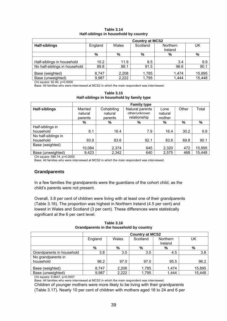
Table 3.14 Half-siblings in household by country
Country at MCS2 Half-siblings England Wales Scotland Northern
Ireland UK
% % % % %
Half-siblings in household 10.2 11.9 8.5 3.4 9.9No half-siblings in household 89.8 88.1 91.5 96.6 90.1
Base (weighted) 8,747 2,208 1,785 1,474 15,895
Chi square: 92.46, p=0.0000 Base (unweighted) 9,987 2,222 1,795 1,444 15,448
Base: All families who were interviewed at MCS2 in which the main respondent was interviewed.
Table 3.15 Half-siblings in household by family type
Family type Half-siblings Married
natural parents
Cohabiting natural parents
Natural parents other/unknown relationship
Lone natural mother
Other Total
% % % % % % Half-siblings in household 6.1 16.4 7.9 16.4 30.2 9.9No half-siblings in household 93.9 83.6 92.1 83.6 69.8 90.1Base (weighted)
10,084 2,374 645 2,320 472 15,895
Chi square: 586.74, p=0.0000 Base (unweighted) 9,423 2,342 640 2,575 468 15,448
Base: All families who were interviewed at MCS2 in which the main respondent was interviewed. Grandparents In a few families the grandparents were the guardians of the cohort child, as the child’s parents were not present. Overall, 3.8 per cent of children were living with at least one of their grandparents (Table 3.16). The proportion was highest in Northern Ireland (4.5 per cent) and lowest in Wales and Scotland (3 per cent). These differences were statistically significant at the 6 per cent level.
Table 3.16 Grandparents in the household by country
Country at MCS2 England Wales Scotland Northern
Ireland UK
% % % % % Grandparents in household 3.8 3.0 3.0 4.5 3.8No grandparents in household 96.2 97.0 97.0 95.5 96.2
Base (weighted) 8,747 2,208 1,785 1,474 15,895
Chi square: 9.9647, p=0.0557 Base (unweighted) 9,987 2,222 1,795 1,444 15,448
Base: All families who were interviewed at MCS2 in which the main respondent was interviewed. Children of younger mothers were more likely to be living with their grandparents (Table 3.17). Nearly 10 per cent of children with mothers aged 16 to 24 and 6 per
39

cent of children with mothers aged 25 to 29 were living with their grandparents. This compares to around 1.5 per cent of those with mothers aged 35 to 39 and 40 and over.
Table 3.17 Grandparents in household by mother’s age at MCS2 interview
16-24 25-29 30-34 35-39 40+ Total % % % % % % Grandparents in household 9.6 6.0 2.3 1.6 1.4 3.5No grandparents in household 90.4 94.0 97.7 98.4 98.6 96.5
Base (weighted) 1,860 2,740 5,155 4,395 1,534 15,683
Chi square: 332.11, p=0.0000 Base (unweighted) 2,151 2,997 4,824 3,875 1,372 15,219
Base: All families who were interviewed at MCS2 in which the main respondent was interviewed and in which the main respondent was a mother (any kind of mother) for whom age was known. Table 3.18 shows variation by ethnicity. Indian (27.5 per cent), Pakistani (18.9 per cent) and Bangladeshi (17.3 per cent) children were the most likely to be living with their grandparents. White children were the least likely to live with grandparents (2.5 per cent). Contact with grandparents not living in the household is discussed in Chapter 4.
Table 3.18
Grandparents in household by child’s ethnic group
White Mixed Indian Pakistani Bangladeshi Black
Caribbean Black
African
Other ethnic group
Total
% % % % % % % % % Grandparents in household 2.5 5.0 27.5
18.917.3 4.8 3.1 6.6 3.7
No grandparents in household 97.5 95.0 72.5 81.1 82.7 95.2 96.9 93.4 96.3Base (weighted) 14,070 468 283 436 128 132 199 189 15,808
Chi square: 845.33, p=0.0000
Base (unweighted) 12,894 446 398 728 278 179 284 260 15,368
Base: All families who were interviewed at MCS2 in which the main respondent was interviewed and in which the cohort child’s ethnic group was known.
Non-resident parents The household grid collects information about which parents were living with the child at three years. Parents who are temporarily away, perhaps working away or abroad, are treated as living with the child. If the child was not living with both of his or her natural parents, additional questions were asked of the main respondent (who was usually the natural mother) about contact with the non-resident parent and maintenance payments received from the non-resident parent. At sweep 2, the questions about maintenance payments were asked only if the non-resident parent was in contact. Almost all non-resident natural parents were natural fathers (rather than natural mothers), so this section looks at non-resident natural fathers only. The natural mother was non-resident in 0.9 per cent of families at sweep 2.
40

Almost all families in which there was a non-resident natural father were lone natural-mother families. However, it could be that the natural mother had found another partner and the child was now living with a stepfather. For this reason this section begins by looking at some correlates of not having a natural father living in the household. It also looks longitudinally at changes in household composition since sweep 12, revealing what proportion of natural fathers who were non-resident at sweep 1 had moved into the household at sweep 2 and the factors associated with making this transition. Finally, the section looks at non-resident parents’ contact with their three-year-olds and (for those non-resident parents who were in contact with their children) at the maintenance payments they made. Natural father in household The proportion of children not living with their natural father increased from 14.1 per cent at sweep 1 to 17.5 per cent at sweep 2. This increase was observed in all countries except Northern Ireland, where the proportion fell from 16.7 per cent to 15.6 per cent, as shown in Table 3.19. A greater proportion of children in England (17.8 per cent) and Wales (19.2 per cent) were not living with their natural father at age three than in Scotland (15.4 per cent) and Northern Ireland (15.6 per cent). Children of younger mothers were most likely to be living apart from their natural father: around 50 per cent of children with mothers aged 16 to 24 and 23.1 per cent of children with mothers aged 25 to 29 did not live with their natural father (Table 3.20). Variations also exist by ethnicity, with 31.8 per cent of Mixed children, 46.9 per cent of Black Caribbean and 32.5 per cent of Black African children living apart from their natural father compared to only 5 per cent of Indian, 9 per cent of Pakistani and 7 per cent of Bangladeshi children (Table 3.21).
Table 3.19 Natural father in household by country
Country at MCS1 Country at MCS2 Natural father in household England Wales Scotland Northern
Ireland UK England Wales Scotland Northern Ireland UK
% % % % % % % % % % Natural father in household 86.4 81.9 85.4 83.3 85.9 82.2 80.8 84.6 84.4 82.5Natural father not in household 13.6 18.1 14.6 16.7 14.1 17.8 19.2 15.4 15.6 17.5Base (weighted) 9,880 2,726 2,302 1,931 18,392 8,841 2,218 1,789 1,480 16,027Base (unweighted) 11,533 2,760 2,336 1,923 18,552 10,107 2,233 1,800 1,450 15,590
MCS1 Chi square: 44.58, p=0.0007 MCS2 Chi square: 15.7829, p=0.0563 Base: All families interviewed at MCS1 Base: All families interviewed at MCS2
2 In a very few families the natural father had died. These families are not excluded from this analysis.
41

Table 3.20 Natural father in household by mother’s age at MCS2 interview
Natural father in household
16-24 25-29 30-34 35-39 40+ Total
% % % % % % Natural father in household 49.7 76.9 88.7 90.9 90.2 82.8Natural father not in household 50.3 23.1 11.3 9.1 9.8 17.2
Base (weighted) 1,864 2,741 5,161 4,399 1,536 15,701
Chi square: 1834.40, p=0.0000 Base (unweighted) 2,155 3,000 4,830 3,877 1,373 15,235
Base: All families who were interviewed at MCS2 in which the main respondent was a mother (any kind of mother) for whom age was known.
Table 3.21 Natural father in household by child’s ethnic group
White Mixed Indian Pakistani Bangladeshi Black Caribbean
Black African
Other ethnic group
Total
% % % % % % % % % Natural father in household 83.2 68.2 95.0 91.0 93.3 53.1 67.5 80.9 82.7Natural father not in household 16.8 31.8 5.0 9.0 6.7 46.9 32.5 19.1 17.3Base (weighted) 14,070 472 285 440 129 132 204 189 15,921
Chi square: 240.52, p=0.0000 Base (unweighted) 12,894 449 401 734 282 180 289 260 15,489
Base: All families who were interviewed at MCS2 in which the cohort child’s ethnic group was known. Transition from non-resident to resident natural father Overall, 19.7 per cent of natural fathers who were not living with their child at sweep 1 had moved into the household with their child by sweep 2 (Table 3.22).
Table 3.22
Transition from non-resident to resident natural father by country
Country at MCS2 Change in natural father in household
England Wales Scotland Northern Ireland
UK
% % % % % Non-resident at MCS1, resident at MCS2 18.5 20.9 25.4 27.9 19.7Non-resident at MCS1 and MCS2 81.5 79.1 74.6 72.1 80.3Base (weighted) 975 355 228 227 1,855
Chi square: 16.58, p=0.0019 Base (unweighted) 1,337 440 255 266 2,298
Base=All families interviewed at MCS1 and MCS2 in which the natural father was non-resident at MCS1. Natural fathers non-resident at sweep 1 were most likely to have moved into the household by sweep 2 in Northern Ireland (27.9 per cent), followed by Scotland (25.4 per cent), Wales (20.9 per cent) and England (18.5 per cent). There were some differences by the mother’s age (Table 3.23). Younger mothers and older mothers
42

were more likely to have moved in with a natural father who was non-resident at sweep 1 – though these differences were not quite statistically significant.
Table 3.23
Transition from non-resident to resident natural father by mother’s age at MCS2 interview
Mother’s age at MCS2 interview (grouped) Change in natural father in household
16-24 25-29 30-34 35-39 40+ Total
% % % % % % Non-resident at MCS1, resident at MCS2 19.5 24.2 17.5 16.0 22.5 19.9Non-resident at MCS1 and MCS2 80.5 75.8 82.5 84.0 77.5 80.1
Base (weighted) 692 419 356 253 103 1,823
Chi square: 11.07, p=0.0575 Base (unweighted) 881 543 414 297 126 2,261
Base: All families interviewed at MCS1 and MCS2 in which the natural father was non-resident at MCS1 and the main respondent at MCS2 was a mother (any kind of mother) for whom age was known. The sweep 1 interview with the main respondent included questions about the non-resident parent. This information can be used longitudinally to look at the characteristics of natural fathers who made the transition from non-residence to residence between sweep 1 and sweep 2. This section looks at three measures from sweep 1; the prior relationship between the parents, frequency of contact between the non-resident father and the child and whether or not the non-resident father paid maintenance. Those families in which the resident natural mother and non-resident natural father were in a relationship at sweep 1 – either ‘closely involved’ or ‘just friends’ – but had not previously lived together were the most likely to have moved in with each other by sweep 2 (24.6 per cent). If the natural mother was ‘not in a relationship’ with the non-resident natural father at sweep 1, they were unlikely to be living together by sweep 2. Indeed, only 7.5 per cent had done so. Of families in which the natural parents had previously lived together or were previously married, 22 per cent had moved in together since sweep 1 (Table 3.24).
Table 3.24
Transition from non-resident to resident natural father by prior relationship from MCS1
Change in natural father in household
Previously married/ lived together
In a relationship
Not in a relationship
Total
% % % % Non-resident at MCS1, resident at MCS2 22.0 24.6 7.5 19.8Non-resident at MCS1 and MCS2 78.0 75.4 92.5 80.2Base (weighted) 809 626 389 1,825
Chi square: 60.32, p=0.0000 Base (unweighted) 945 829 481 2,255
Base: All families interviewed at MCS1 and MCS2 in which the natural father was non-resident at MCS1 and the prior relationship was known from MCS1 main interview. Over a third (35.4 per cent) of non-resident natural fathers who were in contact with their child three or more times a week at nine months had moved into their child’s
43
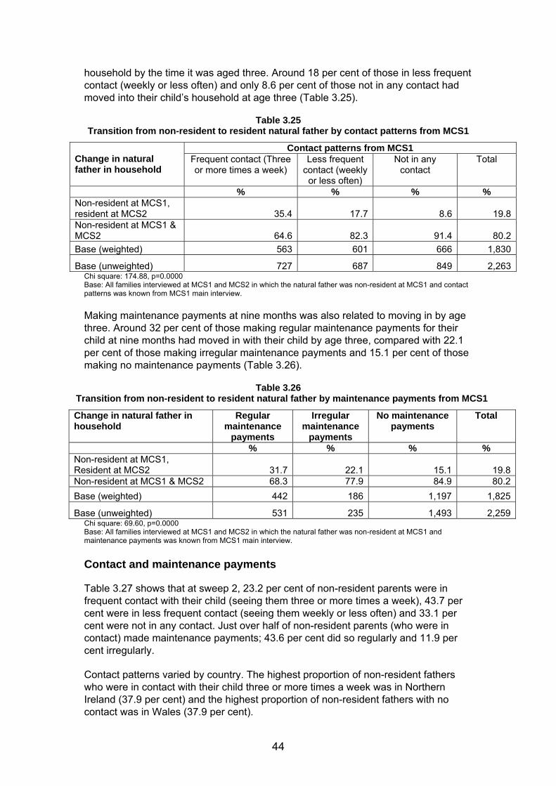
household by the time it was aged three. Around 18 per cent of those in less frequent contact (weekly or less often) and only 8.6 per cent of those not in any contact had moved into their child’s household at age three (Table 3.25).
Table 3.25 Transition from non-resident to resident natural father by contact patterns from MCS1
Contact patterns from MCS1 Change in natural father in household
Frequent contact (Three or more times a week)
Less frequent contact (weekly
or less often)
Not in any contact
Total
% % % % Non-resident at MCS1, resident at MCS2 35.4 17.7 8.6 19.8Non-resident at MCS1 & MCS2 64.6 82.3 91.4 80.2Base (weighted) 563 601 666 1,830
Chi square: 174.88, p=0.0000 Base (unweighted) 727 687 849 2,263
Base: All families interviewed at MCS1 and MCS2 in which the natural father was non-resident at MCS1 and contact patterns was known from MCS1 main interview. Making maintenance payments at nine months was also related to moving in by age three. Around 32 per cent of those making regular maintenance payments for their child at nine months had moved in with their child by age three, compared with 22.1 per cent of those making irregular maintenance payments and 15.1 per cent of those making no maintenance payments (Table 3.26).
Table 3.26
Transition from non-resident to resident natural father by maintenance payments from MCS1
Change in natural father in household
Regular maintenance
payments
Irregular maintenance
payments
No maintenance payments
Total
% % % % Non-resident at MCS1, Resident at MCS2 31.7 22.1 15.1 19.8Non-resident at MCS1 & MCS2 68.3 77.9 84.9 80.2Base (weighted) 442 186 1,197 1,825
Chi square: 69.60, p=0.0000 Base (unweighted) 531 235 1,493 2,259
Base: All families interviewed at MCS1 and MCS2 in which the natural father was non-resident at MCS1 and maintenance payments was known from MCS1 main interview. Contact and maintenance payments Table 3.27 shows that at sweep 2, 23.2 per cent of non-resident parents were in frequent contact with their child (seeing them three or more times a week), 43.7 per cent were in less frequent contact (seeing them weekly or less often) and 33.1 per cent were not in any contact. Just over half of non-resident parents (who were in contact) made maintenance payments; 43.6 per cent did so regularly and 11.9 per cent irregularly. Contact patterns varied by country. The highest proportion of non-resident fathers who were in contact with their child three or more times a week was in Northern Ireland (37.9 per cent) and the highest proportion of non-resident fathers with no contact was in Wales (37.9 per cent).
44

Table 3.27
Contact with non-resident natural father and maintenance payments by non-resident natural father by country
Country at MCS2 Contact and maintenance payments England Wales Scotland Northern
Ireland UK
% % % % % Frequent contact (three or more times a week) 22.4 25.4 24.2 37.9 23.2Less frequent contact (weekly or less often) 44.9 36.8 42.1 29.0 43.7No contact 32.7 37.9 33.7 33.1 33.1Base (weighted) 1,294 419 271 227 2,393Base (unweighted) 1,634 495 296 259 2,684Regular maintenance payments 43.6 41.6 45.7 44.3 43.6Irregular maintenance payments 12.0 11.3 9.6 11.3 11.9No maintenance payments 44.4 47.1 44.7 44.4 44.5Base (weighted) 865 255 179 151 1,589
Contact Chi square: 43.29, p=0.0000 Maintenance Chi square: 1.8211, p=0.9512 Base (unweighted) 1,074 307 193 173 1,747
Base: All families interviewed at MCS2 (except new families) in which the natural father was non-resident and contact patterns/maintenance payments were known from main interview. Contact patterns and maintenance varied with the mother’s age. Younger mothers were less likely to be in contact with the non-resident parent. More than four in 10 (42.3 per cent) of mothers aged 16 to 24 were not in any contact with the non-resident father. Mothers in their thirties were the most likely to receive regular maintenance payments from the non-resident father; around half compared with four in 10 in other age groups (Table 3.28).
Table 3.28
Contact with non-resident natural father and maintenance payments by non-resident natural father by mother’s age
Contact and maintenance payments 16-24 25-29 30-34 35-39 40+ Total
% % % % % % Frequent contact (three or more times a week) 23.5 21.7 24.5 21.8 27.7 23.3Less frequent contact (weekly or less often) 34.2 48.3 47.7 49.8 48.1 43.6Not in any contact 42.3 30.0 27.8 28.3 24.1 33.1Base (weighted) 807 587 514 357 125 2,389Base (unweighted) 952 661 543 380 143 2,679Regular maintenance payments 39.9 38.8 50.8 49.4 39.0 43.6Irregular maintenance payments 10.6 12.7 12.0 12.3 14.1 11.9
No maintenance payments 49.6 48.5 37.2 38.3 46.9 44.5Base (weighted) 463 409 368 254 92 2,587
Contact Chi square: 66.55, p=0.0000 Maintenance Chi square: 24.87, p=0.0202 Base (unweighted) 541 453 381 261 109 1,745
Base: All families interviewed at MCS2 (except new families) in which the natural father was non-resident and contact patterns/maintenance payments were known from main interview and in which main respondent was a mother (any kind of mother) for whom age was known.
45

Table 3.28 Contact with non-resident natural father and maintenance payments by non-resident
natural father by mother’s age Contact and maintenance payments 16-24 25-29 30-34 35-39 40+ Total
% % % % % % Frequent contact (three or more times a week) 23.5 21.7 24.5 21.8 27.7 23.3Less frequent contact (weekly or less often) 34.2 48.3 47.7 49.8 48.1 43.6Not in any contact 42.3 30.0 27.8 28.3 24.1 33.1Base (weighted) 807 587 514 357 125 2,389Base (unweighted) 952 661 543 380 143 2,679Regular maintenance payments 39.9 38.8 50.8 49.4 39.0 43.6Irregular maintenance payments 10.6 12.7 12.0 12.3 14.1 11.9No maintenance payments 49.6 48.5 37.2 38.3 46.9 44.5Base (weighted) 463 409 368 254 92 2,587
Contact Chi square: 66.55, p=0.0000 Maintenance Chi square: 24.87, p=0.0202 Base (unweighted) 541 453 381 261 109 1,745
Base: All families interviewed at MCS2 (except new families) in which the natural father was non-resident and contact patterns/maintenance payments were known from main interview and in which main respondent was a mother (any kind of mother) for whom age was known. Contact patterns and maintenance payments also varied depending on whether the father had become non-resident since sweep 1 or not (Table 3.29). About 83 per cent of non-resident fathers at sweep 2 who were living with their child at sweep 1 were still in contact with their child at age three compared with about 56 per cent of non-resident fathers at sweep 2 who were also non-resident at sweep 1. Of non-resident fathers who were in contact, those who had left the household since sweep 1 were also slightly more likely to pay maintenance – around six in 10 compared with about five in 10 for those who were also non-resident at sweep 1.
Table 3.29 Contact with non-resident natural father and maintenance payments by non-resident
natural father by whether natural father previously resident Contact and maintenance payments
Non-resident natural father in
HH at MCS1
Non-resident natural father not
in HH at MCS1
Total
% % % Frequent contact (three or more times a week) 26.6 21.0 23.2Less frequent contact (weekly or less often) 56.5 35.4 43.7No contact 16.9 43.6 33.1Base (weighted) 937 1,456 2,393Base (unweighted) 928 1,756 2,684Regular maintenance payments 49.7 37.8 43.6Irregular maintenance payments 9.4 14.3 11.9No maintenance payments 41.0 47.9 44.5Base (weighted) 768 821 1,589
Contact Chi square: 211.57, p=0.0000 Maintenance Chi square 27.68, p=0.0001 Base (unweighted) 746 1,001 1,747
Base: All families interviewed at MCS2 (except new families) in which the natural father was non-resident and contact patterns/maintenance payments were known from main interview.
46

Conclusion This chapter presents a picture of both stability and change among the families to which the cohort child belonged. At the age three survey, slightly more than a quarter of the children had gained a younger sibling, and there had been comings and going among the parents with whom they live. Around 6 per cent of families interviewed at both surveys had lost one of two parents present the first time, and 3 per cent had gained a second parent. Well over half the ‘new’ parents were the child’s natural father who had not been resident at sweep 1. Among natural fathers who were not living with the child at sweep 2, two-thirds were reported to be in some form of contact; conversely, one-third had no contact. There are also signs of stabilisation in family life. The proportion of couples that were legally married had gone up, and the vast majority of the cohort families still comprised two natural parents.
47

Chapter 4 THE GRANDPARENTS: WHAT IS THEIR ROLE IN THE FAMILY? Denise Hawkes and Heather Joshi Introduction Grandparents often provide vital financial, emotional and childcare support for their families. They also shape a child’s identity and upbringing, even though, as in the case of the MCS children, they seldom live at the same address. The grandparents’ characteristics are likely to have influenced not only the cohort members’ parents, but the children studied. This chapter provides basic information on the grandparents and offers evidence on some of their roles within the family. Grandparents in the cohort families Table 4.1 presents the proportions of main and partner respondents with two living parents at sweep 2. The cohort child’s mother is usually the main respondent and the father is usually the partner respondent. The table conforms to expectations in two ways. First, both respondents are more likely to have lost their father than their mother. Second, the main respondent is more likely to report each of their parents as living than the partner respondent. This reflects the older age on average of the partner respondent. Main respondents in Northern Ireland are significantly less likely to have a father living than those elsewhere. In addition, partner respondents in Scotland and Northern Ireland are less likely than those in England and Wales to report both parents alive.
Table 4.1 Percentage of respondents with living parents
Main respondent Partner respondent Mother alive 90.4
[89.9-90.9]73.5
[72.3-74.7]Father alive 79.2
[78.3-80.1]63.2
[61.8-64.5]Observations 15,590 12,856Note: Those reporting their parent as dead at MCS1 are accounted for here. Percentages are weighted (using weight 2) and observations are unweighted. Confidence intervals for each cell percentage are presented. This table contains all main respondents and partner respondents. Table 4.2 reports the percentage of living grandparents by main respondents’ ethnicity for those in a two-parent family at sweep 2. For 96 per cent of the two-parent families, both the main and the partner respondents have the same ethnicity. These families almost all have at least one grandparent living. For two-parent families, all of the minority ethnic groups report significantly fewer living grandparents. Only among White respondents do more than half of the families have four living grandparents.
48

Table 4.3 reports the number of living grandparents by main respondent ethnicity for those in a one-parent family at sweep 2. Once again, almost all have at least one parent living, except for a larger proportion within the Black group reporting none. All of the minority ethnic groups have significantly fewer living grandparents and the majority of non-White families live in England.
Table 4.2 Percentage of living grandparents by main respondent ethnicity for couples at sweep 2 White Indian Pakistani/
BangladeshiBlack Other Total
% % % % % % 0 0.1 1.3 1.3 3.5 3.5 0.81 3.8 3.9 7.8 12.7 5.7 4.12 10.6 13.9 17.5 15.9 20.9 11.23 26.8 33.6 33.4 31.2 32.9 27.44 58.2 47.3 40.1 36.7 37.0 56.5
Observations 10,561 354 859 260 304 12,338Note: chi square (16)=226.08, p<0.01. This table contains all main respondents and partner respondents including some evidence from MCS1 where it was missing at MCS2. The cohort child’s mother is usually the main respondent. Those reporting a parent as dead at MCS1 are accounted for here. Percentages are weighted (using weight 2) and observations are unweighted. Ethnicity is that of the main respondent. ‘Black includes all Black groups’ Those who did not respond to the appropriate question in the questionnaire are excluded from the table. New families are excluded.
Table 4.3 Percentage of living grandparents by main respondent ethnicity
for lone parents at sweep 2 White Pakistani/
Bangladeshi Black Other Total
% % % % %
0 2.6 4.0 10.1 5.3 0.81 16.3 36.2 29.9 21.9 4.12 81.2 59.9 60.0 72.8 11.2
Observations 2,117 85 197 73 2,498Note: chi square (8)=72.41, p<0.01. The column for Indian lone mothers has been removed due to the very small sample size. This table contains all main respondents and partner respondents. The cohort child’s mother is usually the main respondent. Those reporting their parent as dead at MCS1 are accounted for here. Percentages are weighted (using weight 2) and observations are unweighted. Ethnicity is that of the main respondent. New families are excluded. Grandparent contact As reported in Chapter 3, just under 4 per cent of the families included resident grandparents, but although they did not live under the same roof, in many cases the two generations of parents saw a lot of each other. For example, 65 per cent of mothers whose own mothers were alive saw them at least weekly and one-fifth saw them daily. Table 4.4 considers the frequency of contact between the respondents and their parents. We observe that both main and partner respondents have more frequent contact with their mother than their father. In addition, main respondents tend to see their parents more often than partner respondents. The main respondents are mostly women, which may explain why they tend to have more frequent contact than partner respondents, who are mainly men.
49

Table 4.4 Contact between respondents and their parents, per cent
Main respondent Partner respondent Contact with Mother Father Mother Father % % % % MCS2
Daily contact 20.5[19.2-21.9]
11.9[11.0-12.9]
6.8 [6.0-7.7]
7.1[6.3-8.0]
Weekly contact 44.8[43.1-46.6
39.5[37.6-41.5]
43.5 [41.1-45.9]
37.5[35.3-39.8]
Monthly contact 26.0[24.1-27.9]
31.8[29.9-33.9]
39.6 [37.2-42.0]
39.3[37.0-41.7]
Yearly or less 6.6[5.8-7.5]
9.5[8.7-10.4]
7.9 [6.9-8.9]
9.8[8.7-10.9]
Never contact 2.1[1.8-2.3]
7.2[6.7-7.8]
2.3 [2.0-2.7]
6.3[5.7-7.0]
Observations 13,997 12,139 9,098 7,722Notes: Daily includes those living with their own parent; this table is constructed for those with a living grandparent
only. The main respondents include lone parents and those with partner respondents. Percentages are weighted (using weight 2) and observations are unweighted.
Confidence intervals for each cell percentage are presented Childcare and financial support from grandparents Table 4.5 describes by partnership status the proportion of families with at least one grandparent undertaking childcare and providing financial help. Around one in four families receives some form of childcare from at least one grandparent and almost all families report some financial help: nine out of 10 couple families and eight out of 10 lone parents. Couples may receive more help of this kind than lone parents because they often have the support of two sets of grandparents rather than one.
Table 4.5 Childcare and financial support provided by at least one grandparent, per cent
At least one grandparent undertaking Any type of child care
Couples 26.1 Lone parent 23.5
Total 25.7 Observations 15,590 Financial help
Couples 90.1 Lone parent 79.5
Total 88.5 Observations 15,406 Note: Child care: chi square (1)=7.32, p=0.037
Financial help: chi square (1)=220.79, p<0.01 Childcare here refers to any type of childcare undertaken since MCS1. Financial support consists of: buying essentials for the baby, paying for other household costs, buying gifts and extras for the baby, paying for childcare and other financial help. Percentages are weighted (using weight 2) and observations are unweighted.
Childcare data have been collected during both sweeps of the MCS. Sweep 1 asked which grandparent was involved, and this was most often the maternal grandmother. Of those using a maternal grandmother as the sole grandparent for childcare at sweep 1, 54.2 per cent were still using such care at sweep 2. However, for those
50

using a mixture of grandparents, maybe but not necessarily including the maternal grandmother, at sweep 1, 46.6 per cent were still using grandparent care at sweep 2. Finally, of those who were not using grandparent care at MCS1, 7 per cent were using it at sweep 2 (table not shown). So we have an impression of substantial but not complete continuity of childcare involving the maternal grandmother, but also of children ‘graduating’ to more formal types of childcare between their first and fourth years.
Table 4.6 Childcare use by working mothers when the children are aged nine months, and child’s cognitive scores at age three BAS Naming Vocabulary Bracken School
Readiness Main form of child care at nine months
Percent Mean 95% confidence interval
Mean 95% confidence interval
100.0 78.3 77.7 78.9 108.9 108.1 109.7Formal group care 22.8 79.0 77.9 80.0 113.2 112.0 114.4Other formal care 17.3 79.4 78.2 80.6 110.1 108.7 111.6
Grandparent 35.4 78.8 78.0 79.7 107.8 106.9 108.7
Partner 19.8 76.4 75.3 77.6 105.7 104.5 106.9Other informal 4.7 74.4 72.4 76.3 105.5 103.5 107.5Observations 5,097 5,097 5,097 5,097 5,097 5,097 5,097 Table 4.6 considers just those families with working mothers at nine months, and looks at outcomes for the children at age three. Grandparent was the most frequent form of childcare reported as the main arrangement by mothers who were then employed, accounting for just over one third of arrangements, with formal group care coming second (23 per cent), and partners third (20 per cent). Other kinds of non–group formal care, such as childminders and nannies, were almost as common (17 per cent) and a small proportion of mothers had made other informal arrangements (5 per cent). Many mothers prefer to leave their baby with a grandparent for reasons of trust, convenience, not to mention cost, but the official cash help associated with childcare credit was not available to compensate care by relatives, in part because of a belief that properly regulated group facilities provided higher standards of care. If formal care is indeed of a higher quality, we might expect the indicators of cognitive development collected at age three to show some variation by the sort of care received at nine months. Although the simple two-way tabulation of the two cognitive scores shown in Table 4.6 does not prove causation, and does not control for other factors which may be associated with type of childcare used and cognitive outcomes (for example, parents’ education), we can see that children who had been in formal group care settings did have higher than average cognitive scores at three. Interestingly, children who had been looked after by grandparents had, on average, almost as high a vocabulary score as those who had attended either type of formal care. They were clearly ahead of children who had been involved in other informal care arrangements, such as those looked after by their father. For the school readiness score (based on children’s understanding of concepts such as colours, letters, numbers/counting, sizes, comparisons and shapes), the group of children with grandparent care are a little further behind those who had been in formal care but still ahead of those with other informal care (Hansen and Hawkes, 2007). This pattern needs further investigation, but it does not immediately suggest that grandparent care of infants leads to any large developmental deficit. In fact, it indicates that it may be particularly beneficial for the acquisition of language.
51

Characteristics of the grandparents Employment in the previous generation At this sweep of the MCS, respondents were asked for the first time about their social origins, a topic held over from sweep 1, where there was not enough room on the questionnaire. To establish whether a question about their parents’ occupation would be relevant, they were asked whether their parents, the present-day grandparents, were working when the respondent was 14 and if so, what that work was. Table 4.7 presents percentages for the main and partner respondent. These reports mainly apply to the 1980s and 1990s. There is little difference between the proportions for the main and partner respondent regarding parental employment. However, we observe that most (around nine out of 10) of the respondents’ fathers were working, compared to a significantly smaller proportion (two-thirds) of the respondents’ mothers. The proportion of fathers is as expected from other data, such as the Labour Force Survey and the Census, on male employment in Britain in the 1980s and 1990s. But the rate for mothers is perhaps a little lower than one would expect from these sources. The shortfall might be because some respondents’ mothers were not in the UK at the time: as Table 4.10 below shows, 15 per cent of respondents were not born in the UK.
Table 4.7
Percentage of respondents whose parents were employed when they were 14 Main respondent Partner respondent
Child’s grandmother worked 66.2[64.8-67.6]
66.7[65.3-68.2]
Observations 15,263 10,316Child’s grandfather worked 86.5
[85.6-87.3]90.0
[89.3-90.8]Observations 14,899 10,104Note: Percentages are weighted (using weight 2) and observations are unweighted. Confidence intervals for each cell percentage are presented. This includes all main and partner respondents who report their parents’ employment. Lone parents are included. Table 4.8 presents these same proportions for the main and partner respondent by country of residence at sweep 2. For all the grandparents, there was least employment reported for those in Northern Ireland.
52

Table 4.8 Percentage of respondents whose parents were employed when they were 14
by country at MCS2 England Wales Scotland Northern
Ireland Chi square
P value UK Confidence
interval Main respondent
Child’s grandmother worked
66.3 67.3 70.2 52.6 Chi square (6) =156.26
66.2 [64.8-67.6]
Observations 9,851 2,184 1,789 1,439 p<0.01 15,263 Child’s grandfather
worked 86.8 84.7 87.3 81.6 Chi square
(6) =42.43 86.5 [85.6-87.3]
Observations 9,851 2,126 1,766 1,426 p<0.01 14,899 Partner respondent
Child’s grandmother worked
67.2 67.0 68.4 50.8 Chi square (6) =126.70
66.7 [65.3-68.2]
Observations 6,757 1,490 1,174 895 p<0.01 10,316 Child’s grandfather
worked 90.3 88.2 89.9 88.2 Chi square
(6) =20.43 90.1 [89.3-90.8]
Observations 6,598 1,456 1,158 892 p<0.01 10,104 Note: Percentages are weighted (using weight 1 for England, Wales, Scotland and Northern Ireland and weight 2 for UK) and observations are unweighted. This includes all main and partner respondents who report their parents’ employment. Lone parents are included.
Social class Table 4.9 presents the social class of the respondent’s parents when he or she was 14, provided that the respondent’s parent was employed. Once again the distribution across the social classes is similar for the main and the partner respondents. However, there are some larger differences between grandmothers and grandfathers. For example, the average percentage of employed grandfathers in managerial or professional jobs was 27 per cent, compared to 16 per cent of the employed grandmothers. At the other end of the scale, 31 per cent of grandfathers and 54 per cent of grandmothers had routine or semi-routine jobs. Looking across the generations, of all the natural mothers at MCS2, 30.1 per cent stayed in the same social class as their own mother, while 30 per cent of all the natural fathers at MCS2 stayed in the same social class as their own father. Further exploration of intergenerational social mobility is now possible, but outside the scope of the Initial Guide.
Table 4.9 Percentage of respondents’ parents within each social class, based on their
occupation when respondents were 14 Natural mothers Natural fathers Mothers’ social class
Managerial and professional 16.9[16.0-17.9]
16.4[15.2-17.8]
Intermediate 19.3[18.3- 20.3]
19.7[18.5-21.0]
Small employers and own-account workers
8.4[7.6-9.4]
8.9[8.0-10.0]
Lower supervisory and technical
0.8 0.8[0.6-1.1] [0.6-1.0]
53

Table 4.9 Percentage of respondents’ parents within each social class, based on their
occupation when respondents were 14 Natural mothers Natural fathers Contd.
Semi-routine and routine 54.6[52.8-56.4]
54.2[52.1-56.2]
Observations 9,295 6,317Fathers’ social class
Managerial and professional 27.6[25.9-29.4]
27.2[25.5-29.4]
Intermediate 9.8[9.0-10.6]
10.2[9.4-11.1]
Small employers and own-account workers
18.1[17.2-19.0]
17.4[16.4-18.5]
Lower supervisory and technical
13.7[12.9-14.7]
14.3[13.3-15.3]
Semi-routine and routine 31.0[29.2-32.4]
30.9[29.1-32.7]
Observations 12,301 8,807Notes: The data for this table are based on an approximation of the SOC codes to the NS-SEC. This table is based on those with employed parents when the respondent was 14. This table contains information on the natural parents of the cohort child. Other parents are excluded from the sample. Percentages are weighted (using weight 2) and observations are unweighted. Confidence intervals for each cell percentage are presented. Family born in UK Table 4.10 considers the country of origin of the respondents and the grandparents. Once again, the differences between the main and partner respondents are rather small. The four main countries of origin for the grandparents born outside of the UK are Pakistan, India, Ireland and Bangladesh. The three top countries of origin for the main respondent born outside the UK are Pakistan, India and Bangladesh. Information on the country of origin for the partner respondent was not collected. The penultimate section of Table 4.10 reports a distribution of year of entry to the UK for the respondents if born outside the UK. Those arriving before 1990 are likely to have spent much of their childhood in the UK. The final section of Table 4.10 considers by country whether the respondent was born in the UK. As expected, England has significantly more respondents born outside the UK than the three Celtic countries.
Table 4.10 Country of origin for respondents and their parents, per cent
Main respondent Partner respondent
Mother born in UK 84.4[82.2-86.4]
84.9[82.5-86.9]
Observations 15,388 10,480
Father born in UK 83.8[81.5-85.9]
84.4[82.0-86.5]
Observations 15,150 10,480
Respondent born in UK 89.7[88.2-91.0]
90.2[88.6-91.6]
Observations 15,447 10,480
54

Table 4.10
Main respondent Country of origin for respondents and their parents, per cent
Partner respondent
Contd. When respondent arrived (if not born in UK)
1950-1969 7.7[6.2-9.5]
13.0[10.9-16.0]
1970-1989 36.0[32.8-39.2]
39.5[35.6-43.5]
1990-2005 56.3[52.9-59.7]
47.5[43.4-51.6]
Observations 2,122 1,394Respondent born in UK (by country)
England 88.7[86.1-89.9]
89.2[87.3-90.8]
Wales 96.3[95.1-97.2]
96.8[95.4-97.7]
Scotland 96.5[95.5-97.3]
95.9[94.3-97.1]
Northern Ireland 95.8[94.1-96.9]
97.7[96.6-98.5]
Chi square (3)=287.03p=0.0000
Chi square (3)=190.83p=0.0000
Observations 15,447 10,480Notes: Percentages are weighted (using weight 2 for UK analysis and weight 1 for country analysis) and observations are unweighted. Confidence intervals for each cell percentage are presented. Conclusion Almost all of the children in the MCS cohort had at least one grandparent still alive at sweep 2, 90 per cent of the families had received financial support from grandparents, and one in four of the families had had some assistance with childcare from grandparents. The children of working mothers who had been looked after by a grandparent at nine months showed similar levels of linguistic development to those who had been in early formal childcare settings. The grandparents themselves were very likely to be employed when the respondent was aged 14 (approximately 90 per cent of fathers and 65 per cent of mothers). These data will enable future analysts to study intergenerational social mobility with the MCS. Finally, more than 80 per cent of the grandparents were born in the UK, with the exceptions most likely to come from Pakistan, India, Ireland and Bangladesh. Reference K. Hansen and D. Hawkes (2006) “The relationship between childcare and cognitive outcomes for children of working mothers”. Mimeo, Centre for Longitudinal Studies, Institute of Education. Paper presented to American Economic Association.
55

Chapter 5 PARENTING Kate Smith Introduction The Millennium Cohort Study provides a rich resource of data on different aspects of parenting, particularly in relation to fathers. Each resident parent was asked a wide range of questions on their activities with their children and their different parenting styles. This information gives a unique picture of what parents do with their children, but also how well they felt they were managing as parents. This chapter is based on the responses of 15,230 main respondents who were mothers (natural, step- or foster), of whom 12,652 were living with partners as a couple or married, and 2,578 were lone mothers. The responses from fathers come from 10,256 natural, step- or foster fathers who were all living in couples and who answered the questionnaire.
Time with child Both mothers and fathers were asked whether they felt they had enough time with their child (Tables 5.1 and 5.2). Two-thirds of mothers said they had plenty of time, compared with only one in four fathers. Five per cent of mothers felt they had nowhere near enough time with their child. In a follow-up question, the majority (76 per cent) said this was due to working long hours. Mothers’ satisfaction with time spent with their child also varied by ethnicity and age. Half of the Black Caribbean mothers felt they had plenty of time, compared to around 86 per cent of Pakistani and Bangladeshi mothers, who, as is shown in Chapter 9, have very low rates of labour force participation. Mothers aged 35 or over were nearly twice as likely to report they had not quite enough or nowhere near enough time with their child (22 per cent) as those aged under 25 (11 per cent). Mothers in families where both parents were employed or where the mother was the only parent in paid work were almost half as likely to report that they had plenty of time with their child (49 per cent and 45 per cent respectively) as mothers who were not in paid work (87 per cent). Mothers in the different UK countries showed no variation in how happy they were with the amount of time they had with their child.
56

Table 5.1 Mothers’ time with child at MCS2
Plenty Percentage (Obs)
Just enough Percentage (Obs)
Not quite enough Percentage (Obs)
Nowhere near enough Percentage (Obs)
Not sure Percentage (Obs)
Total Percentage (Obs)
Total Unweighted Obs
All mothers by ethnic group
% (65)
% (16)
% (15)
% (4)
%
(<1)
%(100) 14,509
White 65 16 15 5 <1 100 12,448Mixed 72 16 7 5 0 100 128Indian 63 17 17 4 0 100 366Pakistani 86 7 5 1 <1 100 649Bangladeshi 87 12 1 0 0 100 245Black Caribbean 51 24 20 6 0 100 176Black African 62 19 15 5 0 100 240Other 68 16 14 1 0 100 257Chi square 130.1563 p value (0.00) All mothers by age
(66) (15) (14) (4) (<1) (100) 15,186
16-24 77 11 9 2 <1 100 2,14525-29 70 14 12 3 <1 100 2,99230-34 65 16 14 5 <1 100 4,81535-39 61 18 17 5 <1 100 3,86540+ 62 16 18 5 <1 100 1,369Chi square 207.894 p value (0.00) All mothers by couples’ employment situation
(66) (15) (14) (4)
(<1) (100) 12,568Two-earner household 49 22 22 7 <1 100 6,668Mother only earner 45 22 25 7 0 100 308Father only earner 87 8 5 1 <1 100 4,627No-earner couple 88 7 4 1 <1 100 965Chi square 1940.076 p value (<0.01)
Notes: Table includes all main respondents who were mothers answering the question who also had valid data on the control variables. Unweighted observations, weighted percentages (using weight 2). Fathers were much more likely than mothers to say they had nowhere near enough time with their child (16 per cent of fathers). This varied by country, with fathers in Northern Ireland less likely to say this than others (Table 5.2). As with mothers, there were variations by ethnicity and age. More than half of Bangladeshi fathers (52 per cent) reported they had plenty of time with their child, compared to 23 per cent of White and Mixed fathers. As for fathers of differing ages, those under 25 were slightly more likely to report they had enough time with their child than those over 25.
57

Like mothers, fathers’ satisfaction with the time spent with their child also varied by working status. More than half of fathers in paid work reported that they had not enough or nowhere near enough time with their child, compared to less than 10 per cent of those not in paid work.
Table 5.2 Fathers’ time with child at MCS2
Plenty Percentage (Obs)
Just enough Percentage (Obs)
Not quite enough Percentage (Obs)
Nowhere near enough Percentage (Obs)
Not sure Percentage (Obs)
Total Percentage (Obs)
Total unweighted
All fathers in couples by country
Per cent (25)
Per cent(23)
Per cent(37)
Per cent(15)
Per cent(<1)
Per cent (100) 10,256
England 24 23 37 16 <1 100 6,707Wales 29 22 35 14 0 100 1,488Scotland 29 22 34 14 <1 100 1,169Northern Ireland 24 28 39 9 0 100 892Chi square 72.98 p Value (0.01) All fathers in couples by ethnic group
(25) (23) (37) (11) (<1)
(100) 9,270
White 23 23 38 16 <1 100 8,114Mixed 23 21 46 9 0 100 64Indian 30 21 37 12 0 100 268Pakistani 42 27 23 7 <1 100 350Bangladeshi 52 22 21 4 1 100 107Black Caribbean 30 24 33 12 1 100 82Black African 25 32 35 8 0 100 103Other 27 26 34 11 2 100 182Chi square 123.73 p value (0.00) All fathers in couples by age
(25) (23) (37) (11) (<1) 100 10,204
16-24 35 28 26 10 1 100 38725-29 28 24 31 17 <1 100 1,29530-34 23 24 37 16 <1 100 2,95335-39 22 22 40 16 <1 100 3,29140+ 28 22 36 14 <1 100 2,278Chi square 120.25 p value (0.00) All fathers by couples’ employment situation
(25) (23) (37) (11) (<1)
100 10,188Two-earner family 21 24 40 16 <1 100 5,610Mother only earner
78 14 6 2 0 100 258
Father only earner
20 23 39 18 <1 100 3,586
No-earner couple 80 12 6 2 1 100 752Chi square 1399.50 p value (0.00)
Notes: Table includes all partner respondents who were fathers answering the question who also had valid data on the control variables. Unweighted observations, weighted percentages (using weight 2 except country analysis which uses weight 1).
58

Family activities Parents were asked about a range of activities they shared with their children (Tables 5.3 and 5.4). Mothers were asked how often they read to their child and whether the child had eaten with the family in the past week. They were also asked if they had managed to do something special for the child’s third birthday and also whether they had been visited by or visited friends with similarly-aged children in the past week. Most mothers read to their child daily (62 per cent) and almost all (92 per cent) read to them at least once a week. Little variation in the frequency with which mothers in the different UK countries read to their child was observed. Bangladeshi, Pakistani and Black African mothers were much less likely to read to their child daily than White mothers, but were just as likely to read at least once a week. This may reflect the cultural norm of storytelling rather than reading to children, or weaker levels of maternal literacy. Mothers over 30 were more likely to read to their child daily than those under 30 (around two-thirds compared to around a half). In households with neither parent in paid work, mothers were least likely to read daily compared to homes with at least one parent in paid work. Almost all children had eaten with their family in the past week (99 per cent) and there was no variation in this across the different groups. This universality also applied to having done something special for the child’s third birthday (97 per cent had a special event for their birthday) and whether they had socialised with families with other young children in the past week (93 per cent had visited or been visited by a family with similar-aged children).
Table 5.3 Mothers reading with their child at age three
Every day Per cent (Obs)
Several times a week Per cent (Obs)
Once or twice a week Per cent Obs)
Once or twice a month Per cent (Obs)
Less often Per cent Obs)
Never Per cent Obs)
Total Per cent
Total unweighted obs
All mothers by ethnic group
(62) (19) (14) (2) (2)
(2)
100 14,541
White 64 19 12 2 1 1 100 12,473Mixed 51 21 12 5 6 4 100 128Indian 46 26 18 1 4 6 100 366Pakistani 37 21 22 3 4 13 100 652Bangladeshi 26 23 28 4 3 15 100 247Black Caribbean 43 27 23 3 2 2 100 178Black African 29 28 30 2 4 7 100 240Other 48 20 18 3 2 10 100 257Chi square 752.71 p value (0.00) All mothers by age
(62) (19) (14) (2) (2) (2) 100 15,671
16-24 50 21 19 4 3 3 100 1,85525-29 54 20 19 3 2 3 100 2,73830-34 65 18 12 2 1 2 100 5,15135-39 66 18 10 2 1 2 100 4,393
59

60
Table 5.3
Every day Per cent (Obs)
Several times a week Per cent (Obs)
Once or twice a week Per cent Obs)
Once or twice a month Per cent (Obs)
Less often Per cent Obs)
Never Per cent Obs)
Total Per cent
Total Mothers reading with their child at age three
unweighted obs
Contd. 40+ 65 19 11 2 1 2 100 1,534Chi square 318.25 p value (0.00) All mothers by couples’ employment situation
(62) (19) (14) (2) (2)
(2)
100 12,587
Two-earner family 67 19 11 2 1 1 100 6,666Mother only earner
58 19 18 2 2 1 100 308
Father only earner 63 18 13 2 1 3 100 4,645No-earner couple 39 20 23 6 4 9 100 968Chi square 499.34 p value (0.00)
Notes: Table includes all main respondents who were mothers answering the question on reading with child who also had valid data on the control variables. Unweighted observations, weighted percentages (using weight 2 except country analysis which uses weight 1). Fathers were also asked how often they read to their child. While they were far less likely than mothers to do this daily (23 per cent), 83 per cent managed to read at least once a week. Fathers were also asked how often they got their child ready for bed and a similar proportion (22 per cent) did so daily as they read to them, which might reflect the traditional practice of the ‘bedtime story’ (Table 5.4). How often fathers in the different UK countries read to their child showed little variation. However, 7 per cent of fathers in Wales never did so, compared to 3 per cent of fathers in Scotland. Bangladeshi fathers were the least likely to read to their child daily (6 per cent) compared to 28 per cent of fathers from the Mixed ethnic group. Older fathers (over 30) were nearly twice as likely to read every day. Around 25 per cent of those over 30 read to their child daily, compared to 13 per cent of those under 25. The differences in daily reading by age for fathers were more marked than those for mothers. Fathers in families where neither parent was in paid work were much less likely ever to read to their child than other fathers:15 per cent never read, which contrasts with just 3 per cent of fathers who were not in paid work, but where the mother was. Fathers only were also asked how often they played with their child. Almost all of them did so daily (78 per cent), with 94 per cent playing at least a few times a week. There was very little variation in this pattern across different groups.

61
Table 5.4 Percentage of fathers reading with the child at age three
Every day (Obs)
Several times a week (Obs)
Once or twice a week (Obs)
Once or twice a month (Obs)
Less often (Obs)
Never (Obs)
Total
Total Unweighted Obs
All fathers in couples by country (23) (27) (32)
(9) (5) (5) 100
10250
England 23 27 32 10 4 5 100 6702 Wales 22 23 33 11 4 7 100 1488 Scotland 26 29 32 7 5 3 100 1169 Northern Ireland 22 25 30 11 7 5 100 891 Chi square 70.16 p value (<0.01) All fathers in couples by ethnic group
(23) (27) (32)
(9) (5) (5) 100
9269
White 24 28 31 9 4 4 100 8113 Mixed 28 27 34 7 1 3 100 64 Indian 17 24 36 10 4 9 100 268 Pakistani 18 15 32 8 8 19 100 350 Bangladeshi 6 22 38 9 11 13 100 107 Black Caribbean 15 18 38 19 8 2 100 82 Black African 10 32 27 11 12 7 100 103 Other 17 28 34 9 5 8 100 182 Chi square 196.79 p value (0.00) All fathers in couples by age
(23) (27) (32) (9) (5) (5) 100 10198
16-24 13 15 47 9 8 8 100 387 25-29 16 21 38 11 6 9 100 1295 30-34 24 28 29 9 4 5 100 2951 35-39 24 29 31 9 4 3 100 3289 40+ 25 26 31 9 4 5 100 2276 Chi square 206.73 p value (0.00) All fathers by couples’ employment situation
(23) (27) (32)
(9) (5) (5) 100
10230
Two-earner family 25 29 31 9 3 3 100 5608

62
Every day (Obs)
Several times a week (Obs)
Once or twice a week (Obs)
Once or twice a month (Obs)
Less often (Obs)
Never (Obs)
Total
Total Unweighted Obs
All fathers in couples by country (23) (27) (32)
(9) (5) (5) 100
10250
Contd. Mother only earner 35 29 27 5 3 3 100 258 Father only earner 21 25 33 11 5 6 100 3583 No-earner couple 15 19 31 9 11 15 100 781
Chi square 337.59 p value (0.00)
Notes: Table includes all partner respondents who were fathers answering the question on reading with child who also had valid data on the control variables. Unweighted observations, weighted percentages (using weight 2 except country analysis which uses weight 1).

Rules Mothers were asked whether their family had many rules and if so, whether they were strictly enforced. Overall, 31 per cent reported that their family had lots of rules, 42 per cent did not have many and 27 per cent reported that it varied. Nearly half reported that their rules were strictly enforced (Tables 5.5 and 5.6). Mothers in Scotland had the most rules (33 per cent reported having ‘lots’ and those in Northern Ireland had the least (25 per cent reporting ‘lots of’ rules). Mothers in Northern Ireland were also the least likely to report rules being strictly enforced, at 41 per cent compared with 50 per cent of mothers in England. Bangladeshi mothers were far less likely than any other ethnic group to report that they had many rules, with only 17 per cent of Bangladeshi mothers compared to 39 per cent of Black Caribbean and Black African mothers reporting ‘lots of’ rules. Pakistani and Bangladeshi mothers were also least likely to say rules were strictly enforced. The number of rules and how strictly these were enforced varied little according to mothers’ age or a couple’s employment situation.
Table 5.5 Mothers’ rules at MCS2, per cent
Lots of rules
Not many rules
Varies
Total
Total unweighted obs
All mothers by country
(31)
(42)
(27)
(100)
15,220
England 31 43 26 (100) 9,801Wales 30 43 27 (100) 2,200Scotland 33 37 30 (100) 1,785Northern Ireland 25 42 33 (100) 1,434Chi square 58.60 p value (<0.001) All mothers by ethnic group (31) (42) (27)
(100) 14,540
White 31 41 27 (100) 12,472Mixed 32 39 29 (100) 128Indian 26 46 29 (100) 366Pakistani 22 57 21 (100) 652Bangladeshi 17 60 23 (100) 247Black Caribbean 39 35 25 (100) 178Black African 36 39 24 (100) 240Other 25 56 19 (100) 257Chi square 80.74 p value (0.00) Notes: Table includes all main respondents who were mothers answering the question on rules with child who also had valid data on the control variables. Unweighted observations, weighted percentages (using weight 2 except country analysis which uses weight 1).
63

Table 5.6 Whether mother reports rules were strictly enforced at MCS2, per cent
Strictly enforced
Not very strictly enforced
Varies
Total percentage
Total unweighted obs
All mothers by country
(49)
(24)
(27)
(100)
15,220
9,801England 50 24 26 (100) 2,200Wales 47 23 30 (100) 1,785Scotland 46 25 29 (100) 1,434Northern Ireland 41 25 35 (100) Chi square 37.0639 p Value (<0.001) All mothers by ethnic group (49) (24) (27)
(100) 14,542
White 51 22 27 (100) 12,474Mixed 45 27 28 (100) 128Indian 43 34 23 (100) 366Pakistani 28 49 23 (100) 652Bangladeshi 28 51 21 (100) 247Black Caribbean 54 22 24 (100) 178Black African 46 23 31 (100) 240Other 38 33 29 (100) 257Chi square 235.94 p value (0.00) Notes: Table includes all main respondents who were mothers answering the question on how strictly rules were enforced with child who also had valid data on the control variables. Unweighted observations, weighted percentages (using weight 2 except country analysis which uses weight 1). Parenting style Both parents were also asked about their style of parenting. Overall, mothers were fairly evenly split between reporting ‘firm discipline with lots of fun’ (43 per cent) and ‘doing the best for my child’ (48 per cent). Fathers were more likely to report that their style was ‘firm discipline with lots of fun’ (54 per cent). See Table 5.7. Variations by country and ethnicity were found. Mothers in Northern Ireland were more likely to report ‘doing their best for their child’ than those elsewhere (63 per cent compared to 47 per cent of mothers in England). Pakistani mothers (and those from unspecified ‘other’ minority ethnic groups) were less likely to report that their style involved ‘firm discipline and lots of fun’ (under 30 per cent each) compared to 49 per cent of Black Caribbean mothers. However, they were particularly likely to report ‘doing the best for their child’.
Table 5.7 Mothers’ parenting style at MCS2, per cent
Firm rules and discipline
Lots of fun
Not really thought about it
Firm rules with fun
Doing my best
Total
Total unweighted obs
All mothers by country
(2) (5) (2) (42)
(50) (100) 14,723
England 2 5 2 44 47 (100) 9,350Wales 2 5 2 41 50 (100) 2,165Scotland 2 5 2 40 51 (100) 1,780
64

Table 5.7
Firm rules and discipline
Lots of fun
Not really thought about it
Firm rules with fun
Doing my best
Total
Total Mothers’ parenting style at MCS2, per cent
unweighted obs
Contd. Northern Ireland
2 3 1 31 63 (100) 1,428
Chi square 144.58 p value (0.001) All mothers by ethnic group
(2) (5) (1) (42)
(50) (100) 14,095White 2 5 1 44 48 (100) 12,411Mixed 1 4 2 42 48 (100) 118Indian 2 4 3 43 48 (100) 293Pakistani 5 6 4 28 57 (100) 536Bangladeshi 6 9 3 34 48 (100) 179Black Caribbean
4 5 5 49 42 (100) 176
Black African 8 3 <1 45 43 (100) 187Other 3 7 2 29 58 (100) 195Chi square 192.01 p value (0.001)
Notes: Table includes all main respondents who were mothers and answered the question on their parenting style with child who also had valid data on the control variables. Unweighted observations, weighted percentages (using weight 2 except country analysis which uses weight 1). Unlike the mothers, there was little variation in fathers’ parenting styles (Table 5.8) by country, age, or family employment status. There was some variation, however, by fathers’ ethnic group. Bangladeshi fathers were the least likely to report ‘firm discipline with lots of fun’ as a parenting style: only 30 per cent reported this, compared with 60 per cent of Black Caribbean fathers.
Table 5.8 Fathers’ parenting style at MCS2, per cent
Firm rules and discipline
Lots of fun
Not really thought about it
Firm rules with fun
Doing my best
Total
Total unweighted obs
All fathers in couples by ethnicity
(3) (7) (4) (54)
(33) (100) 9,254
White 2 7 4 54 32 (100) 8,108Mixed 3 6 3 65 24 (100) 64Indian 1 11 2 49 38 (100) 268Pakistani 8 11 1 38 42 (100) 347Bangladeshi 6 21 4 30 40 (100) 107Black Caribbean 4 7 2 60 28 (100) 81Black African 6 4 1 56 33 (100) 103Other 4 7 2 42 46 (100) 176Chi square 107.01 p value (<0.01)
Notes: Table includes all partner respondents who were fathers and answered the question on their parenting style with child who also had valid data on the control variables Unweighted observations, weighted percentages (using weight 2 except country analysis which uses weight 1).
65
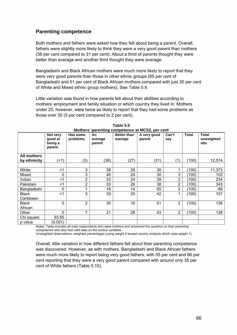
Parenting competence Both mothers and fathers were asked how they felt about being a parent. Overall, fathers were slightly more likely to think they were a very good parent than mothers (36 per cent compared to 31 per cent). About a third of parents thought they were better than average and another third thought they were average. Bangladeshi and Black African mothers were much more likely to report that they were very good parents than those in other ethnic groups (65 per cent of Bangladeshi and 51 per cent of Black African mothers compared with just 30 per cent of White and Mixed ethnic group mothers). See Table 5.9. Little variation was found in how parents felt about their abilities according to mothers’ employment and family situation or which country they lived in. Mothers under 25, however, were twice as likely to report that they had some problems as those over 30 (5 per cent compared to 2 per cent).
Table 5.9 Mothers’ parenting competence at MCS2, per cent
Not very good at being a parent
Has some problems
An average parent
Better than average
A very good parent
Can’t say
Total
Total unweighted obs
All mothers by ethnicity
(<1)
(3) (38) (27) (31)
(1) (100) 12,574
White <1 3 38 28 30 1 (100) 11,373Mixed 0 3 40 24 30 3 (100) 102Indian <1 2 33 24 39 2 (100) 234Pakistani <1 2 33 26 38 2 (100) 343Bangladeshi 0 1 18 14 65 3 (100) 89Black Caribbean
<1 3 33 20 42 1 (100) 157
Black African
0 2 30 16 51 2 (100) 138
Other 0 7 21 28 43 2 (100) 138Chi square 93.85 p value (0.001)
Notes: Table includes all main respondents who were mothers and answered the question on their parenting competence who also had valid data on the control variables. Unweighted observations, weighted percentages (using weight 2 except country analysis which uses weight 1). Overall, little variation in how different fathers felt about their parenting competence was discovered. However, as with mothers, Bangladeshi and Black African fathers were much more likely to report being very good fathers, with 55 per cent and 66 per cent reporting that they were a very good parent compared with around only 35 per cent of White fathers (Table 5.10).
66

Table 5.10 Fathers’ parenting competence at MCS2, per cent
Not very good at being a parent
Has some problems
An average parent
Better than average
A very good parent
Can’t say
Total
Total unweighted obs
All fathers in couples by ethnicity
(1)
(3) (28) (32) (36)
(1)
(100) 8,946
White 1 3 28 33 35 1 (100) 7,993Mixed 2 7 21 31 34 6 (100) 61Indian 1 3 18 34 43 1 (100) 241Pakistani 1 2 26 22 47 2 (100) 272Bangladeshi 1 0 17 27 55 0 (100) 64Black Caribbean
1 3 17 27 50 2 (100) 75
Black African
2 0 10 26 63 0 (100) 84
Other 1 7 24 18 53 2 (100) 150Chi square 85.29 p value (0.00)
Notes: Table includes all partner respondents who were fathers and answered the question on their parenting competence who also had valid data on the control variables. Unweighted observations, weighted percentages (using weight 2 except country analysis which uses weight 1). Regular bedtimes Overall, around 80 per cent of mothers reported that the cohort child usually or always had a regular bedtime and only 7 per cent said they never or almost never had one. Mothers in Wales were nearly twice as likely as those in Scotland to report that their child never or almost never had a regular bedtime (9 per cent compared to 5 per cent respectively). See Table 5.11. There was also some variation by ethnicity. This ranged from 17 per cent of Black Caribbean mothers reporting a regular bedtime always, compared to 44 per cent of White mothers. Mothers in households where they were in paid work and their partner was not and those in families where neither parent was working were nearly twice as likely to report that their child never or almost never had a regular bedtime as mothers in couples where both parents worked.
Table 5.11 Regularity of bedtimes at age three, per cent
Never (Obs)
Sometimes (Obs)
Usually (Obs)
Always (Obs)
Total
Total unweighted obs
All mothers by country
(7) (12) (38) (43)
(100) 15,220
England 7 13 38 43 (100) 9,802Wales 9 11 34 46 (100) 2,200Scotland 5 11 43 40 (100) 1,785
67

Table 5.11
Never (Obs)
Sometimes (Obs)
Usually (Obs)
Always (Obs)
Total
Total unweighted
Regularity of bedtimes at age three, per cent
obs Contd. Northern Ireland 7 12 41 41 (100) 1,433Chi Square 67.36 p value (0.00) All mothers by ethnic group
(7) (12) (38) (43)
(100) 14,541
White 7 11 39 44 (100) 12,473Mixed 14 16 40 30 (100) 128Indian 5 22 37 36 (100) 366Pakistani 8 25 30 37 (100) 652Bangladeshi 5 27 34 34 (100) 247Black Caribbean 10 26 47 17 (100) 178Black African 13 27 38 22 (100) 240Other 8 26 40 27 (100) 257Chi square 283.33 p value (0.00) All mothers by couple’s employment situation
(7) (12) (38) (43)
(100) 12,587Two-earner family
5 10 42 43 (100) 6,666
Mother only earner
12 16 37 35 (100) 308
Father only earner
7 13 36 45 (100) 4,645
No-earner couple
13 20 31 36 (100) 968
Chi square 216.61 P value (0.00) Notes: Table includes all main respondents who were mothers and answered the question on the child’s regular bedtimes who also had valid data on the control variables Unweighted observations, weighted percentages (using weight 2 except country analysis which uses weight 1). Mealtimes Almost all mothers reported that their child usually or always had regular mealtimes (92 per cent). As with bedtimes, the regularity of mealtimes varied by mothers’ age. The youngest mothers were twice as likely to report that regular mealtimes only happened sometimes as those aged 30-34 (11 per cent compared to 5 per cent). See Table 5.12. Mothers in Northern Ireland were most likely to report that their child always had regular meal times: 54 per cent, compared to 47 per cent in England. Around one in four Black African mothers reported that their child always had a regular mealtime, compared to nearly half of Indian and White mothers.
68

Table 5.12 Regularity of mealtimes at MCS2, per cent
Never
Sometimes
Usually
Always
Total
Total unweighted obs
All mothers by country
(2) (7) (45)
(47)
(100) 15,220
England 2 7 45 47 (100) 9,802Wales 3 7 39 52 (100) 2,200Scotland 1 4 47 48 (100) 1,785Northern Ireland 1 5 40 54 (100) 1,433Chi square 101.98 p value (0.00) All mothers by ethnic group
(2) (7) (45)
(47)
(100) 14,542
White 2 6 45 49 (100) 12,473Mixed 5 9 41 45 (100) 128Indian 2 11 40 48 (100) 366Pakistani 4 16 38 42 (100) 652Bangladeshi 5 15 43 37 (100) 247Black Caribbean 1 16 47 37 (100) 178Black African 6 14 53 27 (100) 240Other 3 14 48 35 (100) 257Chi square 245.72 p value (0.00) All mothers by age
(2) (7) (45)
(47)
(100) 13,837
16-24 3 11 41 45 (100) 2,14725-29 2 8 41 49 (100) 2,99630-34 1 6 45 49 (100) 4,82035-39 1 4 46 48 (100) 3,87440+ 2 7 51 40 (100) 1,372Chi square 177.14 p value (0.00)
Notes: Table includes all main respondents who were mothers and answered the question on the child’s regular mealtimes who also had valid data on the control variables. Unweighted observations, weighted percentages (using weight 2 except country analysis which uses weight 1). Parenting beliefs and values English-speaking mothers were asked to rate which of a set of qualities they thought was the most important to instil in their child, as shown in Table 5.13. Overall, half of mothers reported that the most important quality they would like their child to have was the ability to ‘think for themselves’ (Table 5.13). Mothers in Northern Ireland displayed distinct differences to their counterparts elsewhere. Nearly twice as many mothers in Northern Ireland thought it was important to obey parents as in the other UK countries. Twenty per cent of mothers in Northern Ireland thought this was important, compared to 9 per cent in Scotland and 11 per cent in England and Wales. Differences according to ethnic group also emerged. Pakistani, Bangladeshi and Black African mothers were much less likely to report that ‘thinking for themselves’ was the most important quality for their child to have than White mothers (17 per cent compared to 52 per cent of White mothers). Learning religious values was selected as most important by 30 per cent of Black African mothers and 24 per cent of Pakistani mothers, but by only 2 per cent of White mothers.
69

The youngest mothers (under 24) were more likely to think it was important that their child obeyed their parents than those over 35 (15 per cent compared to 9 per cent). There was little variation in the qualities that mothers in different family employment situations wished to instil in their child.
Table 5.13 Most important qualities for children at MCS2, per cent
To be well liked/ popular
To think for themselves
To work hard
To help others
To obey parents
To learn religious values
Total
Total unweighted obs
English-speaking mothers by country
(5) (50) (13) (19) (11)
(3) (100) 14661
England 5 50 13 19 11 3 (100) 9,310Wales 5 47 15 20 11 2 (100) 2,152Scotland 3 55 12 19 9 2 (100) 1,778Northern Ireland 2 40 13 20 20 6 (100) 1,421Chi square 257.13 p value (0.00) English-speaking mothers by ethnic group
(5) (50) (13) (19) (11)
(3) (100) 13,998
White 5 52 12 19 10 2 (100) 12,329Mixed 6 39 19 13 15 8 (100) 117Indian 6 37 24 15 14 4 (100) 291Pakistani 4 18 17 15 22 24 (100) 534Bangladeshi 7 17 18 17 22 18 (100) 174Black Caribbean 2 41 11 13 20 13 (100) 176Black African 3 20 21 10 17 30 (100) 185Other 2 36 16 15 20 19 (100) 192Chi square p value English-speaking mothers by age
(5) (50) (13) (19) (11)
(3) (100) 13,334
16-24 2 39 19 21 15 2 (100) 2,08425-29 3 46 16 18 14 3 (100) 2,83230-34 5 51 12 20 10 3 (100) 4,64635-39 6 54 10 18 9 3 (100) 3,77240+ 4 55 10 18 9 5 (100) 1,317Chi square 360.18 p value (0.00)
Notes: Table includes English-speaking main respondents who were mothers and answered the question on the most important quality they would like their child to have who also had valid data on the control variables. Unweighted observations, weighted percentages (using weight 2 except country analysis which uses weight 1). English-speaking mothers were also asked to say whether they would wish to instil a range of values in their children, including independence, obedience and respect, the art of negotiation, respect for elders, doing well at school and religious values. There was almost no variation for the first five values, with virtually all mothers wanting to impart these. There was much more variation, however, over whether they wished to instil religious values in their child (Table 5.14).
70

Mothers in Northern Ireland reported very different views on this issue than their counterparts in the other UK countries. Eighty-five per cent of mothers in Northern Ireland wished their child to have religious values, compared with around 50 per cent elsewhere in the UK. There was even more variation by ethnicity and age of mothers, with more than 90 per cent of Asian and Black mothers saying they wished to instil these values in their child, compared to 54 per cent of White mothers. Sixty-eight per cent of mothers over 40 wished to instil religious values, compared to 38 per cent of mothers under 24. There was very little variation in the values that mothers in different family employment situations wished to instil in their child.
Table 5.14
Important values for children, per cent Independence
(Obs)
Obedience and respect (Obs)
Art of negotiation (Obs)
Respect for elders (Obs)
Doing well at school (Obs)
Religious values (Obs)
Total unweighted obs
English-speaking mothers by country
(99) (99) (97) (100) (99) (56) 14,634
England 99 99 97 100 99 56 9,282Wales 100 99 97 100 100 52 2,157Scotland 100 99 97 100 99 52 1,773Northern Ireland
100 100 97 100 100 85 1,422
Chi square 565.08p value (0.00)English-speaking mothers by ethnic group
(99) (99) (97) (100) (99) (56) 14,006
White 100 99 97 100 99 54 12,363Mixed 100 96 97 99 100 68 118Indian 97 99 96 100 100 90 287Pakistani 97 99 96 100 100 98 523Bangladeshi 92 100 96 100 100 94 171Black Caribbean
100 100 93 99 100 86 175
Black African 98 100 96 100 100 96 180Other 99 99 94 98 99 77 189Chi square 552.47p value (0.00)English speaking-mothers by age
(99) (99) (97) (100) (99) (56) 14,624
16-24 99 99 95 99 100 38 2,07525-29 99 99 97 100 100 48 2,83130-34 100 100 97 100 99 58 4,63735-39 100 99 98 100 99 64 3,76640+ 99 99 97 99 99 68 1,315Chi square 446.17p value (0.00)
Notes: Table includes English-speaking main respondents who were mothers and answered whether they wished to instil the range of values in their child and who also had valid data on the control variables. Unweighted observations, weighted percentages (using weight 2 except country analysis which uses weight 1).
71

Conclusion The evidence presented here shows many similarities in parenting practice and beliefs across mothers and fathers and also across the types of families distinguished here: by country in the UK, ethnic group, age at interview, and couples’ employment status. How working parents are coping is a question of general concern and interest. While most mothers felt they had enough time with their child, working mothers were more likely than others to say they could do with more time, but on most other measures of parenting, they were no different from other mothers. In fact, two-earner families were the group most likely to read to their child regularly, which provides indirect evidence that maternal employment does not eliminate the chance to carry out this activity with the child. Employed fathers, who are more likely than employed mothers to be working full-time and for long hours, were most likely to feel they were not able to spend enough time with their child. Fathers in general were less likely to report reading daily to their child than mothers, but this happened least in families with no parent in paid work. Otherwise there was little difference in parenting behaviour among fathers with and without jobs. With these data, more research could be done on such issues as parental employment patterns and hours worked, and the effect on the amount of time parents felt they have with their child and other family activities. Future analyses will also be able explicitly to compare the experiences of mothers and fathers in couples with those parenting alone. Other clear differences in parenting style reveal themselves across different groups of mothers and fathers, whether employed or not. An interesting question is whether these systematic and individual differences will be differentially related to children’s behaviour and achievement later on. This is something that MCS data will be able to reveal in the future.
72

Chapter 6 CHILD HEALTH Carol Dezateux, Alice Sullivan, Summer Sherburne Hawkins, Tim Cole, and Heather Joshi Introduction The Millennium Cohort Study provides an important opportunity to examine health and illness in the context of children's lives, families, and social and environmental circumstances. This can help us to understand how social experience can affect health outcomes. This chapter expands on child health themes addressed in earlier reports, focusing on outcomes relevant to child development, disability and longstanding conditions, as well as children’s experiences of injuries and immunisation. It uses one of the largest national exercises to collect the height and weight of children to assess how many, and who, were overweight or obese. We present findings according to health outcome and conclude with a brief review of emerging inequalities of gender, geography, ethnicity and social disadvantage. As we noted earlier, this is the first opportunity to examine longitudinal questions in the MCS, and here we present a preliminary exploration of the influence of circumstances in infancy on health at the age of three. These data provide a rich source of information about the distribution of indicators of child health and ill-health across the four UK countries and according to area-based measures of social disadvantage and (in England) minority ethnic population. Although one in three families had changed address between sweeps 1 and 2, most had not moved more than two kilometres. Even though some families were no longer living in the same type of ward by sweep 2 (a minority yet to be quantified), the following tables do reflect the type of area in which the cohort children spent the first year of life, and the circumstances of that year may still have a bearing on their later development. First-year death rates were significantly higher than the national average in the minority ethnic wards in our survey (nine per 1,000) but quite close to the average in other survey wards (six per 1,000 in disadvantaged wards and five per 1,000 elsewhere). Most of these infant deaths occurred in the first month of life, and virtually all of them before the survey was conducted at nine months (Cullis, 2007). Throughout this chapter, as elsewhere in the report, we simplify matters by looking only at children who are singletons. In addition, we selected only main respondents who were mothers, and partners, where present, who were fathers. Where analyses of health outcomes at three years are examined in relation to exposures at nine months, these tables include only children interviewed on both occasions.
73

74
Healthy development As expected, the great majority of three-year-olds had achieved major motor milestones indicating normal healthy development. For example, almost all had succeeded in walking since the previous interview, with virtually all able to walk without difficulty (99.6 per cent) and almost as many able to ‘walk up steps like an adult, one foot on each step’ (96.5 per cent). However, there was somewhat more variation in toilet training (Table 6.1). Parents reported 83 per cent of the children as always ‘dry by day’ and ‘clean by day’. The highest percentages always clean and dry by day were recorded for children in Northern Ireland, especially those in less disadvantaged areas, and the lowest percentage in England (Table 6.1). Significant differences existed between boys and girls: only 77.9 per cent of boys were always dry by day compared with 88.0 per cent of girls, with similar figures for always clean by day (Table 6.2). This may have important implications for gender differences in early access to day care and nursery education, where toilet training may be necessary for access, and warrants further exploration. There were significant variations across ethnic groups, with the mothers of Bangladeshi children reporting systematically lower percentages always clean or always dry by day (75 to 76 per cent) than Whites (83 to 84 per cent), and Indians reporting more (88 to 89 per cent). See Table 6.3. Overall, 13.4 per cent of mothers reported concerns about their children’s speech and language development (Table 6.1). The patterns by area-level measures of disadvantage were not consistent between countries, with mothers from disadvantaged areas of Wales and Scotland being more likely to report concerns than those in advantaged areas in those countries. In Northern Ireland, however, mothers in non-disadvantaged areas were more likely to have concerns. No such differences were observed in England; however, mothers from areas with a high proportion of minority ethnic residents were least likely to report concerns. Gender differences were also observed. Mothers were more likely to have concerns about boys’ speech (17.1 per cent) than girls’ (9.6 per cent). See Table 6.2. Variation in the proportion expressing concerns about children’s speech according to ethnic group was not statistically significant (Table 6.3).

Table 6.1 Toilet training and concern about speech by country and type of ward at MCS1
England England England Wales Wales Scotland Scotland N. Ireland N. Ireland UK
Type of ward at MCS1
Not disadvantaged
Dis- advantaged
Minority ethnic
Not disadvantaged
Dis- advantaged
Not disadvantage
d
Dis- advantage
d
Not disadvantaged
Dis- advantaged Total
Chi square
(p value)
Always dry by day 82.4 82.4 81.4 87.6 86.9 84.7 83.3 89.1 84.0 82.9
22.32
(0.002) Unweighted n 4,137 3,764 1,878 677 1,536 914 861 570 836 15,173 Always clean by day 82.77 83.47 84.1 86.71 86.9 84.56 84.88 87.54 84.09 83.47
13.65 (0.0438)
Unweighted n 4,137 3,762 1,881 677 1,534 913 860 570 836 15,170 Any concerns about speech? 13.7 13.6 12.2 9.9 13.5 11.4 13.5 17.5 16.0 13.4
13.61 (0.0299)
Unweighted n 4,140 3,765 1,884 677 1,536 915 861 571 836 15,185
Table 6.2 Toilet training and concerns about speech by gender
Male Female
Total Chi square (p value)
Always dry by day 77.9 88.0 83.0 272.99Unweighted n 7,723 7,450 15,173 (<0.0001) Always clean by day 78.2 88.9 83.5 313.98Unweighted n 7,726 7,444 15,170 (<0.0001) Concerns about speech 17.1 9.6 13.4 183.38 (<0.0001)Unweighted n 7,734 7,451 15,185
75
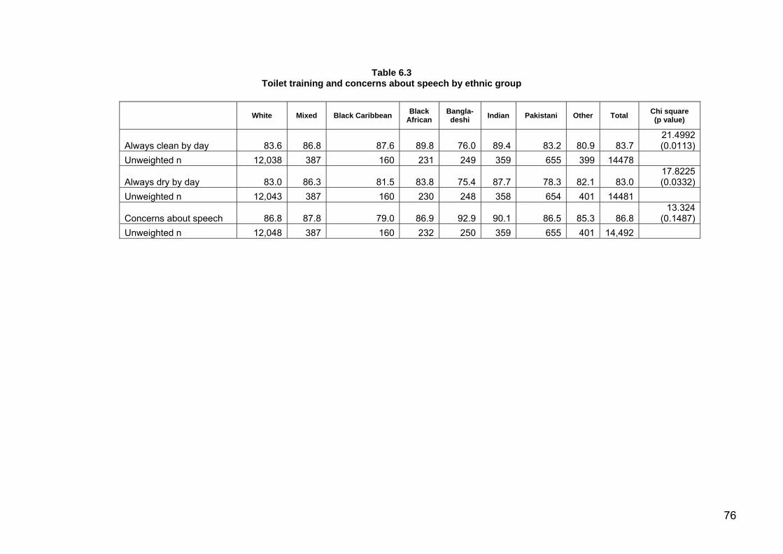
76
Table 6.3 Toilet training and concerns about speech by ethnic group
White Mixed Black Caribbean Black African
Bangla-deshi Indian Pakistani Other Total Chi square
(p value)
Always clean by day 83.6 86.8 87.6 89.8 76.0 89.4 83.2 80.9 83.721.4992 (0.0113)
Unweighted n 12,038 387 160 231 249 359 655 399 14478
Always dry by day 83.0 86.3 81.5 83.8 75.4 87.7 78.3 82.1 83.017.8225 (0.0332)
Unweighted n 12,043 387 160 230 248 358 654 401 14481
Concerns about speech 86.8 87.8 79.0 86.9 92.9 90.1 86.5 85.3 86.813.324
(0.1487) Unweighted n 12,048 387 160 232 250 359 655 401 14,492

77
Disability and general health Overall, mothers reported a long-term condition lasting three months or more and diagnosed by a health professional in one in six children (15.8 per cent). This was more common among boys (16.7 per cent) than girls (14.9 per cent). See Table 6.4.
Table 6.4 Longstanding illness by children’s gender
Male Female Total Chi square (p value)
Longstanding illness (per cent) 16.7 14.9 15.88.99
(0.0202) Unweighted n 7,733 7,451 15,184
Table 6.5 shows rates were significantly lower in Northern Ireland (within original ward type) and for those in minority ethnic areas in the first survey. Problems with vision and hearing in the early years are important as they can influence early development or social interaction. Overall, one in 16 (6 per cent) of mothers reported a problem with their children’s sight: this was more common for those in disadvantaged communities (Table 6.5). This is consistent with a UK-wide study of severe visual impairment or blindness using the Carstairs Index (Rahi et al, 2003). Although the latter study also found a significantly higher incidence of eye problems in all minority ethnic children compared to their White counterparts, there was no significant difference in such problems among three-year-olds in MCS by ethnicity. Only 33 children were registered blind or partially-sighted: however, this is likely to represent only the most severe visual loss, and to omit unregistered but visually impaired children who will nevertheless be excluded from sighted/print education. A problem with hearing was reported for one in 20 children (4.8 per cent) but did not show a consistent pattern according to ward type (Table 6.5).

78
Table 6.5 Longstanding illness and parental concerns about eyesight, hearing, by country and type of ward at MCS1
England England England Wales Wales Scotland Scotland N. Ireland N. Ireland UK
Type of ward at MCS1
Not dis-advantaged
Dis-advantaged
Minority ethnic
Not dis-advantaged
Dis-advantaged
Not dis-advantage
d
Dis-advantaged
Not dis-advantaged
Dis-advantaged Total
Chi square
(p value)
Long-term illness 15.6 17.4 13.2 13.4 16.9 14.0 17.3 11.0 15.0 15.8
20.89 (0.0145)
Unweighted n 4,139 3,765 1,884 677 1,536 915 861 571 836 15,184
Any problem with eyes 6.1 7.1 5.3 4.9 8.3 6.1 7.1 4.7 8.8 6.4
12.62
(0.0458)
Unweighted n
4,122
3,735 1,875 676 1531 912 861 569 834 15,115
Any problem with hearing 5.5 4.4 3.3 4.0 5.3 2.6 2.8 4.4 4.0 4.8
27.67 (0.0001)
Unweighted n
4,111 3737 1,878 671 1,526 913 859 567 833 15,095
Note: Longstanding illness defined as a condition lasting three months or more and diagnosed by a health professional

Among those with a long-term condition, about one in five (or 3 per cent of all children) was limited in playing or from joining in other activity normal for his/her age. Such conditions were more common in children from disadvantaged communities across all four UK countries and, in England, were least common in areas of high minority ethnic prevalence (Table 6.5). This was more marked by ethnic group: there was a two-fold variation in the frequency of longstanding conditions that mothers reported. These were more prevalent by the age of three in Black Caribbean children (18.7 per cent) and least common in Black African children (8.8 per cent), and were significant in univariable analyses, even though numbers in some groups were small. Table 6.6 shows the weighted sample size as well as the actual number of cases, as a reminder that the composition of the sample over-represents some minority ethnic groups, such as Bangladeshi, Pakistani and Indian children.
Table 6.6 Longstanding illness by ethnic group
White Mixed Black Caribbean
Black African
Bangla-deshi Indian Pakistani Other Total Chi square
(p value)
Longstanding illness 16.0 16.5 18.7 8.8 9.3 10.3 14.9 15.5 15.8
16.763100442
Unweighted n 12,048 387 160 232 250 359 655 401 14,492weighted n 13,088 409 117 166 115 257 392 360 1,4904
The frequency of longstanding conditions did not vary significantly by family poverty as assessed during infancy (Table 6.7) but children with longstanding conditions were more likely to be limited in play or activity if their family income was below 60 per cent of median equivalised income. Similar patterns were observed when income at sweep 2 was examined.
Table 6.7 Longstanding illness at three by family income at sweep 1
Above 60 per cent median equivalised income
Below 60 per cent median equivalised income
Total p value
Family income at nine months Longstanding illness 15.8 15.5 15.7 Unweighted n 9632 4076 13708 0.7053Among those with longstanding illness: Limiting condition 16.9 24.7 18.5 Unweighted n 1493 636 2,129 0.005 Family income at three years Longstanding illness 15.9 17.2 16.2 Unweighted n 7177 3244 12395 0.1167Among those with longstanding illness Limiting condition 16.9 24.7 18.7 Unweighted n 1301 664 1974 .0000
79

Asthma and acute illnesses Overall, by the age of three, one in 10 children was reported as having had asthma (Table 6.8). In univariable analyses, this was significantly more common among boys (13.8 per cent) than girls (9.6 per cent). Wheezing or whistling in the chest in the preceding 12 months was reported for 30.5 per cent of children, and this was also significantly more common among boys (Table 6.8). Asthma and wheezing or whistling in the chest in the preceding 12 months were more common in children in disadvantaged communities in all four UK countries (Table 6.9). Children of Afro- Caribbean origin were more likely to have had asthma or to have experienced wheezing by the age of three, and those of Bangladeshi origin least likely (Table 6.10). Asthma and wheezing were significantly more common among children whose mothers had smoked in pregnancy (Table 6.11). This may reflect differences in airway development as well as in response to infection since, at this age, the symptoms of viral-associated wheezing are not readily distinguishable from asthma. Overall, 37 per cent of children were reported to have eczema and/or hay fever, but these two questions were inadvertently combined during fieldwork programming, hence the prevalence at MCS2 of these conditions cannot be reported separately. Chickenpox was reported in 45.6 per cent of children and was more common in girls (47.0 per cent) than boys (44.3 per cent). See Table 6.8. In each UK country, chickenpox was more common in advantaged communities (Table 6.9) and was particularly low in areas of high minority ethnic prevalence. White mothers were more likely to report a history of chickenpox in their child. Overall, 6.5 per cent of children had recurrent ear infections and, in Wales and Scotland, this was more common in disadvantaged communities, while in England it was lowest in areas with relatively more minority ethnic groups (Table 6.9). Children of Black African ethnicity were least, and White children most, likely to have such infections, but these differences are not statistically significant overall. Recurring ear infections are thought to reflect several environmental exposures including parental smoking, which is socially and ethnically patterned (Table 6.10). Exposure to tobacco in utero or during early foetal life was associated with an increased frequency of ear infections – 7.8 per cent compared with 6.0 per cent in the unexposed (Table 6.11).
80

81
Table 6.8
Asthma and wheezing, chickenpox and recurring ear infections by gender
Male Female Total
Chi square (p value)
Asthma 13.8 9.6 11.7 62.3527
(<0.0001)Unweighted n 7,602 7,343 14,945
Wheezing in chest 33.8 27.1 30.5 78.6838
(<0.0001)Unweighted n 7,733 7,451 15,184 Chickenpox 44.3 47.0 45.6 10.98280(0038)
Recurring ear infections 7.71 5.60 6.68 26.9913(0.0001)
7,718 7444 15,162 Unweighted n 7,652 7,388 15,040
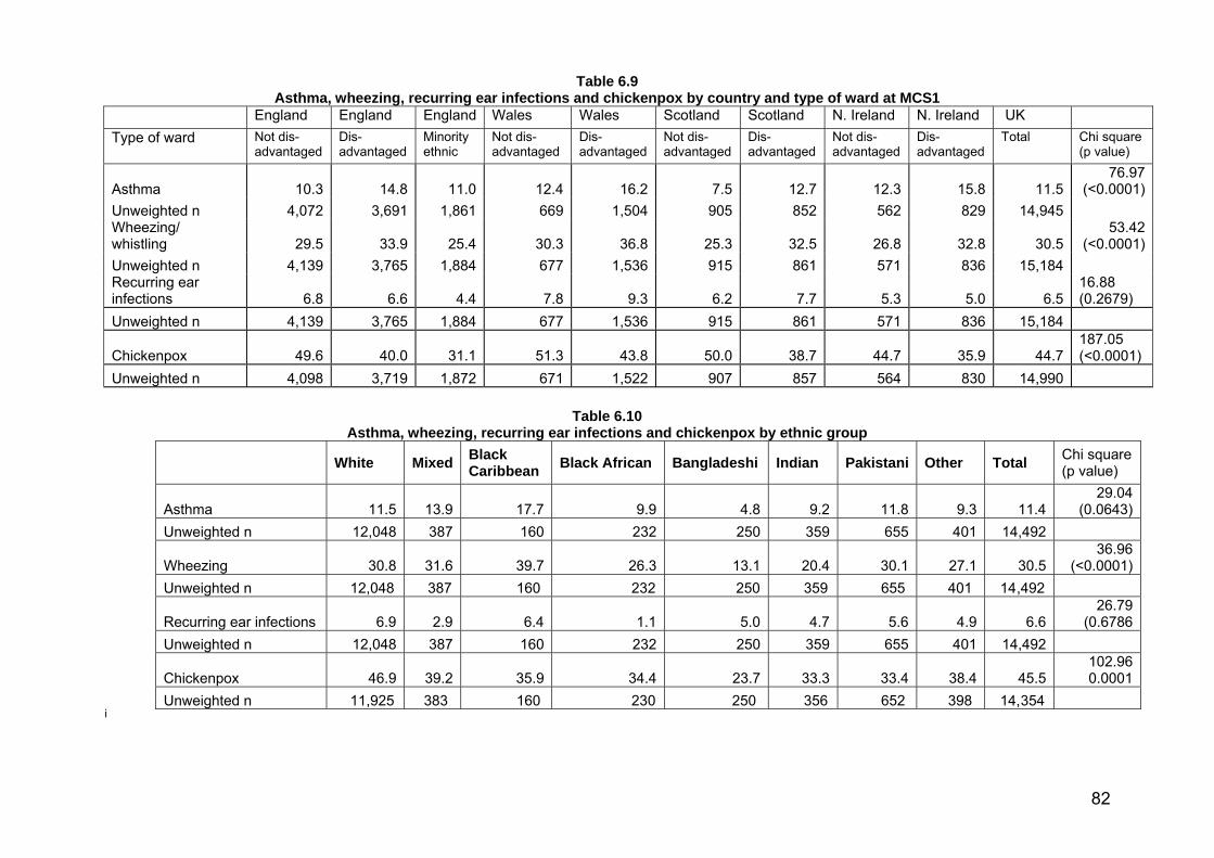
82
Table 6.9 Asthma, wheezing, recurring ear infections and chickenpox by country and type of ward at MCS1
England England England Wales Wales Scotland Scotland N. Ireland N. Ireland UK Type of ward Not dis-
advantaged Dis-advantaged
Minority ethnic
Not dis-advantaged
Dis-advantaged
Not dis-advantaged
Dis-advantaged
Not dis-advantaged
Dis-advantaged
Total Chi square (p value)
Asthma 10.3 14.8 11.0 12.4 16.2 7.5 12.7 12.3 15.8 11.576.97
(<0.0001) Unweighted n 4,072 3,691 1,861 669 1,504 905 852 562 829 14,945 Wheezing/ whistling 29.5 33.9 25.4 30.3 36.8 25.3 32.5 26.8 32.8 30.5
53.42 (<0.0001)
Unweighted n 4,139 3,765 1,884 677 1,536 915 861 571 836 15,184 Recurring ear infections 6.8 6.6 4.4 7.8 9.3 6.2 7.7 5.3 5.0 6.5
16.88 (0.2679)
Unweighted n 4,139 3,765 1,884 677 1,536 915 861 571 836 15,184
Chickenpox 49.6 40.0 31.1 51.3 43.8 50.0 38.7 44.7 35.9 44.7187.05 (<0.0001)
Unweighted n 4,098 3,719 1,872 671 1,522 907 857 564 830 14,990
Table 6.10 Asthma, wheezing, recurring ear infections and chickenpox by ethnic group
White Mixed Black Caribbean Black African Bangladeshi Indian Pakistani Other Total Chi square
(p value)
Asthma 11.5 13.9 17.7 9.9 4.8 9.2 11.8 9.3 11.429.04
(0.0643) Unweighted n 12,048 387 160 232 250 359 655 401 14,492
Wheezing 30.8 31.6 39.7 26.3 13.1 20.4 30.1 27.1 30.536.96
(<0.0001) Unweighted n 12,048 387 160 232 250 359 655 401 14,492
Recurring ear infections 6.9 2.9 6.4 1.1 5.0 4.7 5.6 4.9 6.626.79
(0.6786 Unweighted n 12,048 387 160 232 250 359 655 401 14,492
Chickenpox 46.9 39.2 35.9 34.4 23.7 33.3 33.4 38.4 45.5102.96 0.0001
Unweighted n 11,925 383 160 230 250 356 652 398 14,354
i

83
Table 6.11 Child asthma, wheezing and recurring ear infections by maternal smoking
Mother smoked in pregnancy
No Yes Total Chi square (p value)
Asthma 9.9 14.5 11.4 65.96
(<0.0001)Unweighted n 9,875 4,758 14,633
Wheezing or whistling in the chest 27.9 35.8 30.4 91.75
(<0.0001)Unweighted n 9,875 4,758 14,633
Recurring ear infection 6.0 7.8 6.5 16.33
(0.0004)Unweighted n 9,346 4,904 14,250
Health service attendance for accidental injury By three years of age, 35.4 per cent of children were reported to have had at least one accidental injury requiring admission to hospital, attendance at an accident and emergency department or a health centre (Table 6.12). This was more common in boys (39.4 per cent) than girls (31.3 per cent). The chance of suffering such injury was significantly greater for those in the disadvantaged areas of each country, but showed little difference between countries for a given level of area disadvantage and was lowest among those in areas of high minority ethnic group prevalence (Table 6.13). In univariable analyses, accidental injuries were significantly more common among White children (Table 6.14). There was a strong association with family poverty when measured either at nine months or at three years (Table 6.15): 39.9 per cent of children living in families with net equivalised income below 60 per cent of the national median experienced at least one significant injury by sweep 2.
Table 6.12 Health service attendance for accidental injury by child gender
Males Females TotalChi square
(p value)
39.4 31.3 35.49.30
(<0.0057)Unweighted n 7,734 7,450 15,184

84
Table 6.13 Health service attendance for accidental injury by country and type of ward at MCS1
England England England Wales Wales Scotland Scotland N. Ireland N. Ireland UK Type of ward Not dis-
advantaged Dis-advantaged
Minority ethnic
Not dis-advantaged
Dis-advantaged
Not dis-advantaged
Dis-advantaged
Not dis-advantaged
Dis-advantaged
Total Chi square (P Value)
Accidental injury prompting health service attendance 34.1 38.6 26.0 38.9 39.1 34.4 40.3 34.5 36.1 35.4
76.3494 (<0.0001)
Unweighted n 4,140 3,765 1,884 676 1,536 915 861 571 836 15,184
Table 6.14
Health service attendance for accidental injury by ethnic group
White Mixed Black Caribbean
Black African
Bangla deshi Indian Pakistani Other Total Chi square
(p value) Accidental injury prompting health service attendance 36.4 33.3 30.7 24.8 22.8 22.7 25.7 25.0 35.2
72.88(<0.0001)
Unweighted n 12,048 387 160 232 250 359 655 401 14,492
Table 6.15 Health service attendance for accidental injury at MCS2 by family income at nine months and three years
Above 60 per cent
median equivalised income
Below 60 per cent median equivalised income
Total
Income at nine months
35.3 38.23 36.0 9.77(<0.0051)
Unweighted n 9,780 4,157 13,937Income at three years
34.3 39.9 36.5 22.04 (0.0001)
Unweighted n 8,602 4,376 12,578

85
Immunisation Since 1988, children in the UK have been offered the combined measles, mumps and rubella vaccine (MMR) at 13 months of age and again before school entry. Some parents have used separate vaccines for their children, fearing that the combined MMR vaccine might be linked to autism and bowel disease, although evidence for this is lacking. Single vaccines are available only privately and the extent of their use is unknown. Parents were asked to report their child’s immunisation, and were prompted to confirm this using their three-year-old’s personal child health record if this was available. Overall, 6 per cent of children did not receive any immunisation against MMR (Table 6.16). This varied by gender, with fewer girls (5.6 per cent) than boys (6.5 per cent) completely unimmunised. Combined MMR vaccine was given to 88 per cent of children, while 6 per cent received at least one vaccine separately. The proportion of children receiving the combined MMR vaccine was lowest in England compared with other UK countries (Table 6.17). Within England, use of combined MMR vaccine was highest among those in disadvantaged areas and in areas of high minority ethnic group prevalence, while elsewhere in the UK there was no difference according to area-level indicators. Use of single vaccines was highest in families from non-disadvantaged areas of England (7.8 per cent). Use of combined MMR was lowest and use of single vaccines highest in infants of White, Mixed or other ethnicity (Table 6.18). Conversely, use of combined MMR was highest among those from ethnic groups of the Indian subcontinent and Black Africans. The association of maternal educational level with MMR is complex (Table 6.19): mothers lacking qualifications or those with NVQ level 3 and above were more likely to have a completely unimmunised infant, while those with higher educational qualifications were more likely to use at least one single vaccine. In univariable analyses, single parents and couples (both natural parents) had similar rates of take-up of the MMR vaccine. However, single parents were less likely to use at least one single vaccine (2.7 per cent compared to 6.5 per cent). Therefore, the children of single parents were slightly more likely to be unvaccinated (table not shown).
Table 6.16 Immunisation for measles, mumps and rubella by gender
Male Female Total Chi square (p value)
None 6.5 5.6 6.1 4.93 (0.0305) Unweighted n 7,734 7,451 15,185
Combined MMR vaccine 87.5 89.1 88.310.20
(0.0077) Unweighted n 7,734 7,451 15,185
At least one separately 6.0 5.2 5.64.64
(0.0978) Unweighted n 7,734 7,451 15,184

Table 6.17
Immunisation for measles, mumps and rubella by country and type of ward at MCS1
England England England Wales Wales Scotland Scotland N. Ireland N. Ireland UK Type of ward Not dis-
advantaged Dis-advantaged
Minority ethnic
Not dis-advantaged
Dis-advantaged
Not dis-advantaged
Dis-advantaged
Not dis-advantaged
Dis-advantaged
Total Chi square (P Value)
Immunisation for measles, mumps or rubella
None 5.6 6.8 7.6 6.6 9.0 5.7 6.0 3.3 4.7 6.1 19.58 (0.0575)
Combined MMR vaccine 86.6 89.7 89.9 89.2 88.0 90.9 91.4 94.1 94.1 88.3
55.81 (0.0002)
At least one separately 7.8 3.5 2.5 4.2 3.0 3.4 2.6 2.6 1.2 5.6
149.23 (0.0001)
Total unweighted n 4,140 3,765 1,884 677 1,536 915 861 571 836 15,185
Table 6.18
Immunisation by children’s ethnic group
White Mixed Black Caribbean
Black African Bangladeshi Indian Pakistani Other Total Chi square
(p value)
Immunisation for measles, mumps or rubella (MMR)
None 5.9 8.9 10.5 4.7 6.8 3.6 6.5 8.1 6.116.3254 0.0214
Combined MMR 87.9 85.7 88.6 93.6 92.0 92.3 93.3 87.2 88.155.8132 0.0029
At least one vaccine separately 6.2 5.4 0.9 1.8 1.3 4.1 0.3 4.6 5.8 Total unweighted n 12,048 387 160 232 250 359 655 401 14,492
86

87
Table 6.19 Immunisation for measles, mumps and rubella by mothers’ highest education level
No qualifications
NVQ level1
NVQ level2
NVQ level3
NVQ level4
NVQ level5
Other/ overseas
Don’t know
Total Chi square (p value)
None 8.2 4.5 5.4 6.3 6.3 7.0 5.0 6.7 6.1 21.07(0.0211)
Combined MMR
90.5 93.3 90.4 86.9 85.1 83.5 92.6 90.9 88.3119.17
(0.0001)At least one separately
1.4 2.2 4.2 6.8 8.6 9.5 2.4 2.4 5.8 190.1411(0.0001)
Total unweighted n
1,906 1,152 4,084 2,144 4,170 561 436 695 15,148

88
Childhood obesity Weight problems and obesity have been increasing in the UK in recent decades, even among pre-school children. The Health Survey for England from 1995 to 2002 found the proportion of overweight (including obese) children had risen from 17 to 22 per cent in boys aged two to five and from 20 to 25 per cent in girls (Stamatakis et al, 2002). Obese children risk increased health problems, such as type 2 diabetes and high blood pressure, as well as psychosocial difficulties, including low self-esteem (Lobstein et al, 2004). They are also more likely to be obese in adolescence and adulthood (Power et al, 1997). It is estimated that obesity and its consequences cost the NHS more than £1 billion per year (UK Parliament, 2004). Tackling childhood obesity is a cross-Government priority. In 2004, the Departments of Health, Education and Skills, and Culture, Media, and Sport created a joint public service agreement target to halt the yearly rise in obesity among children under age 11 by 2010 (Department of Health, 2004).
Children from the Millennium Cohort Study were weighed and measured in sweep 2 by interviewers newly trained for this purpose. The attempt to measure so many children in their own homes at such a young age was ambitious, but it provided an opportunity to examine the prevalence of overweight and obesity within this contemporary cohort of UK children. Body Mass Index (BMI; weight/height squared), a proxy for adiposity, is the most common measurement of body size at the population level. Childhood overweight and obesity is defined by the International Obesity Task Force cut-offs for BMI (Cole et al 2000). These cut-offs were based on data from six countries, including the UK, and the centiles are linked to the widely accepted adult cut-offs for overweight and obesity. Hence data can be compared internationally Height and weight data at three years were visually inspected for outliers by plotting height, weight, height vs weight, and BMI distributions as well as identifying values classified as biologically implausible for weight-for-age, height-for-age, or BMI-for-age. Cases were excluded if deemed biologically implausible (488) or a height and/or weight value was missing (820). Data are presented on 13,771 singleton children with complete and plausible height/weight/BMI data and where the main or partner informant was the natural, adoptive, or step- parent. This sample is composed of children from both sweep 1 (13,195) and the boosted sample at MCS2 (576). All exposure variables are based on data collected at the first contact, unless otherwise specified; however, families from the boosted sample have data available from the second contact only. Unweighted frequencies and weighted percentages are presented.

Table 6.20 Overweight and obesity by country at MCS1: unweighted frequencies (weighted per cent)
England Wales Scotland N. Ireland Total p value
Normal weight 6,896 (77.8) 1,482 (72.9) 1,221 (75.7) 944 (73.2) 10,543 (76.3)Overweight (excluding obesity) 1,506 (17.5) 418 (21.9) 310 (19.2) 270 (20.8) 2,504 (18.7)
Obesity 453 (4.8) 108 (5.2) 87 (5.1) 76 (6.0) 724 (5.0)Unweighted n 8,855 2,008 1,618 1,290 13,771 P<.001
Note: MCS2 singleton children with valid data.
Table 6.21 Overweight and obesity by country and type of ward at MCS1: unweighted frequencies (weighted per cent)
England:
Advantaged
England: Dis-
advantaged
England: Minority ethnic
Wales: Advantaged
Wales: Dis-
advantaged
Scotland: Advantaged
Scotland: Dis-
advantaged
N. Ireland: Advantaged
N. Ireland: Dis-
advantagedTotal p value
Normal weight
2,969 (78.4)
2,585 (75.8)
1,342 (80.8) 432 (71.3) 1,050 (74.9) 639 (76.3) 582 (74.6) 381 (73.3) 563 (73.1) 10,543 (77.2)
Overweight (excluding obesity)
658 (17.4) 628 (18.4) 220 (13.3) 145 (23.9) 273 (19.5) 163 (19.5) 147 (18.9) 107 (20.6) 163 (21.2) 2,504 (18.0)
Obesity 158 (4.2) 196 (5.7) 99 (6.0) 29 (4.8) 79 (5.6) 36 (4.3) 51 (6.5) 32 (6.2) 44 (5.7) 724 (4.8) Total n
(unweighted) 3,785 3,409 1,661 606 1,402 838 780 520 770 13,771 p<.001
Note: MCS2 singleton children with valid data.
Table 6.22 Overweight and obesity by children’s gender: unweighted frequencies (weighted per cent)
Male Female Total p value Normal weight 5405 (77.9) 5138 (76.5) 10543 (77.2)
Overweight (excluding obesity) 1221 (17.7) 1283 (18.2) 2504 (18.0)
Obesity 339 (4.4) 385 (5.3) 724 (4.8)Unweighted n 6,965 6,806 13,771 p=.06
Note: MCS2 singleton children with valid data.
89

90
Table 6. 23 Overweight and obesity by child’s ethnicity: unweighted frequencies (weighted per cent)
White Mixed Indian Pakistani Bangladeshi Black Caribbean
Black African
Other Total p value
Normal weight 8724 (76.8) 302 (78.4) 325 (90.8) 513 (82.5) 176 (80.6) 111 (67.6) 170 (72.7)
189 (80.6) 10,510 (77.2)
Overweight (excluding obesity)
2,207 (18.6) 70 (16.7) 28 (5.4) 82 (12.1) 21 (8.2) 22 (15.0) 40 (16.6) 25 (13.5) 2,495 (18.0)
Obesity 571 (4.6) 21 (4.8) 11 (3.8) 35 (5.4) 23 (11.2) 21 (17.5) 26 (10.7) 14 (6.0) 722 (4.8) Unweighted n 11,502 393 364 630 220 154 236 228 13,727 p<.001
Note: MCS2 singleton children with valid data.
Table 6.24 Overweight and obesity by MCS2 equivalised family income: unweighted frequencies (weighted per cent)
Above 60% median
Below 60% median
Total p value
Normal weight 6159 (77.6) 2806 (76.8) 8965 (77.4)
Overweight (excluding obesity)
1499 (18.2) 637(17.4) 2136 (18.0)
Obesity 375 (4.2) 209 (5.8) 584 (4.6)Unweighted n 8033 3652 11685 p=.009
Table 6.25.
Overweight and obesity by highest academic qualification at MCS1: unweighted frequencies (weighted per cent) Degree Diploma A/AS/S
levels GCSE
grades A-C or above
GCSE grades D-G or below
Other academic
qualification
None of these
qualifications
Total p value
Normal weight 1,842 (78.7)
950 (77.7) 1,049 (80.1) 3,534 (77.1) 1,067 (74.0) 287 (77.8) 1,793 (74.9) 10,522 (77.2)
Overweight (excluding obesity)
428 (17.6) 227 (17.2) 215 (16.0) 889 (18.5) 272 (19.1) 52 (16.6) 414 (18.5) 2,497 (18.0)
Obesity 98 (3.7) 64 (5.1) 60 (3.9) 228 (4.4) 91 (6.9) 22 (5.6) 161 (6.6) 724 (4.9)Unweighted n 2,368 1,241 1,324 4,651 1,430 361 2,368 13,743 p<.001
Note: MCS2 singleton children with valid data.

At sweep 1, 2,504 (18.0 per cent) of MCS children were overweight and 724 (4.8 per cent) were obese. Patterns for each exposure variable are described by combining overweight and obesity because of the small numbers in each ‘obesity’ cell. Children from Wales, Scotland, and Northern Ireland were more likely to be overweight or obese than children from England (Table 6.20). Similar patterns were seen by UK country and type of ward (Table 6.21). Fewer children were overweight or obese in England, specifically those from electoral wards classified as ‘ethnic’. Overall, there was a slightly higher prevalence of overweight or obesity in children from ‘disadvantaged’ wards in England and Scotland (the upper quartile of the Child Poverty Index) than ‘advantaged’ wards (all remaining wards). There were no statistically significant differences in overweight or obesity between boys and girls (Table 6.22); however, the prevalence of overweight or obesity varied by ethnic group (Table 6.23). Indian children had the lowest prevalence of overweight or obesity (9.2 per cent), while Black Caribbean children had the highest (32.5 per cent). There were also differences by family income (Table 6.24) and the mothers’ highest academic qualification (Table 6.25). Children from families with income below a line drawn at roughly 60% of the national median equivalised income were slightly but significantly more likely to be overweight or obese than children where family income is above that line. Children whose mothers had a degree, diploma, A/AS/S levels, GCSE grades A-C or above, or ‘other’ qualification, were less likely to be overweight or obese than children whose mothers had lower or no qualifications. Training unspecialised interviewers to weigh and measure nearly 14,000 children in the home has produced one of the largest such datasets in the UK. The results can be linked to a wealth of information about the child, their family and the place where they live. We have shown that just under a quarter of three-year-old children from the MCS were overweight or obese and there is evidence of social and ethnic patterning. These findings can assist the Government in tackling childhood obesity by helping to inform public health policy. Conclusion This preliminary look at the health data collected at age three from children in the Millennium Cohort Study suggests that while the majority of pre-school children in the four UK countries are healthy, there is nonetheless significant inequality in health outcomes as delineated by area and individual measures of social disadvantage, ethnicity and income. While the variations in health between groups as measured by social disadvantage are striking, this confirms well-established evidence. A striking finding has been that of marked variations in a range of health outcomes by the age of three years according to the characteristics of the communities in which the children live. Thus, children starting out in disadvantaged areas are more likely to experience disability and ill-health in the form of problems with vision, hearing and longstanding conditions, asthma, chronic infections and injuries and are more likely to be obese or overweight. These inequalities merit further analyses to inform strategies to improve children’s health and well-being.
91

There is not a systematic tendency for poor or good health, on the indicators used here, in the children recruited to the survey in areas of high minority ethnic settlement. Most of the children in these areas belonged to minority ethnic groups. When we analyse the sample by the ethnicity of all children in the survey, whether or not they came from these areas, a degree of ethnic diversity in health conditions becomes apparent, and helps to explain why living in one of the ethnic areas is not a simple predictor of good or bad child health. Despite the raised chances of infant deaths in these places, the first survey has shown that mothers from at least some minority groups are more likely than Whites to breastfeed and less likely to smoke. This may account for the lower frequency of certain health problems among some minority ethnic children, for instance asthma and wheezing among Bangladeshi children. These preliminary analyses also suggest that there is considerable ethnic variation in overweight or obesity: this needs to be interpreted with caution as Body Mass Index does not distinguish those who are heavy for their height because of their muscle rather than fat. Furthermore, we have observed some early and important differences between boys and girls. Thus, relative to girls, boys are more likely to be delayed in toilet training and speech, and are more likely to have wheezing and asthma and to require medical attention for injuries, and are less likely to receive the combined MMR vaccine, while, relative to boys, girls are more likely to have chickenpox. Interestingly, we found no gender differences in the prevalence of overweight and obesity at age three. The variations we have observed may relate to different social expectations and early social experiences and could in turn influence access to early-years provision and later health. Further exploration of these gender differences is warranted. Acknowledgements Summer Sherburne Hawkins is funded through a Department of Health Researcher Development Award. Tim Cole is funded through an MRC programme grant G9827821. References Cole, T.J., Bellizzi, M.C., Flegal, K.M. and Dietz, W. H. (2000) ‘Establishing a standard definition for child overweight and obesity worldwide: International survey’. BMJ, 320:1240. Cullis, A. (2007) Infant mortality in the Millennium Cohort Study sample areas. CLS Technical Report, London: Centre for Longitudinal Studies. Department of Health (2004) National Standards, Local Action: Health and Social Care Standards and Planning Framework 2005/6-2007/8. London. Lobstein, T., Baur, L. and Uauy, R. (2004) ‘Obesity in children and young people: a crisis in public health.’ Obesity Review 2004-05 (supplement 1):4-85.
92

Power, C., Lake, J.K., Cole, T.J. (1997) ‘Measurement and long-term health risks of child and adolescent fatness.’ International Journal of Obesity, 21: 507-526 Rahi, J.S., Cable, N. British Childhood Visual Impairment Study Group, ‘Severe visual impairment and blindness in children in the UK’, Lancet. 2003; 362:1359-65 Stamatakis, E. ‘Anthropometric measurements, overweight, and obesity’. In Sroston, K. and Primatesta, P., eds. Health Survey for England 2002: The Health of Children and Young People, Vol 1. London: The Stationery Office. UK Parliament: House of Commons Health Committee (2004) Obesity. Third Report of session 2003-04. Vol 1. London: The Stationery Office.
93

Chapter 7 CHILD DEVELOPMENT
Anitha George, Kirstine Hansen and Ingrid Schoon3
Introduction Child developmental assessments, even very early in life, have been found to be good indicators of future educational performance and levels of health. If early outcomes are differentially related to demographic and socio-economic factors, this may establish inequalities early in life. These, in turn, promote or limit children’s paths through life, depending on the families into which they are born (Schoon, 2006). In this chapter we describe the measures assessing child outcomes at age three and examine the factors that contribute to differences in developmental adjustment at this age. Child outcomes at age three have been measured by two cognitive assessments: the naming vocabulary subtest of the British Ability Scales (BAS) and the School Readiness Composite (SRC) of the Revised Bracken Basic Concept Scale. In addition, child behaviour was assessed using the Strengths and Difficulties Questionnaire (SDQ). The BAS Naming Vocabulary subtest is part of a cognitive test battery designed for children aged between three and 17 years (Elliott, 1983). The test is individually administered. The interviewer asks the child to name a series of pictures of everyday items. There are 36 items in total, although the number each child is asked about is dependent on their performance. The assessment is terminated if five successive items are answered incorrectly. BAS assesses the expressive language ability of children. It was not administered to children who do not speak English. The School Readiness Composite (SRC) comprises six subtests of the Revised Bracken Basic Concept Scale measuring children’s knowledge of those ‘readiness’ concepts that parents and teachers traditionally teach children in preparation for formal education (Bracken, 1998). This assessment is also individually administered. The test has been designed for children in the age range of two-and-a-half to seven years and 11 months. The six subtests of the SRC comprise the assessment of children’s basic concepts such as colours, letters, numbers/counting, sizes, comparisons and shapes. As a non-verbal test, requiring the child to point, but not speak, it could be given in oral translation to children who do not speak English. Both cognitive assessments were administered using Computer Assisted Personal Interviewing (CAPI) by interviewers who were specially trained but were not professional psychologists. Altogether each assessment was administered to over 12,000 children (not necessarily all the same individuals. The results reported in this chapter cover 12,096 children’s responses to the BAS Naming Vocabulary subtest and of 11,553 to the Bracken SRC test. This is after discarding cases where the respondents were not the child’s parents, and the second and third child in sets of twins and triplets.
3 With additional material on language in the home contributed by Dina Dimou
94

The analysis used BAS and SRC normed scores, derived from standard BAS and Bracken tables and defined with reference to the standardisation samples used in developing the assessments; these scores have also been adjusted according to the age of the cohort child. These analyses have not, as yet, been adjusted for contextual information about the circumstances of the assessment. For assessing emotional and behavioural problems of the children, the Strengths and Difficulties Questionnaire (SDQ) was used. The SDQ is a behavioural screening questionnaire for three- to 16-year-olds (Goodman, 1997, 2001; Goodman, Meltzer, & Bailey, 1998) and is a well-validated tool for screening psychiatric disorder. It consists of 25 items generating an overall scale score as well as scores for five subscales measuring conduct problems, hyperactivity, emotional symptoms, peer problems and pro-social behaviour. The items were assessed via parental report (normally by the mother), in the computer-assisted self-completion module. For the following analysis an overall difficulties mean score for the whole sample was computed by summing replies to the subscales indicating problematic behaviour, i.e. conduct problems, hyperactivity, emotional symptoms, and peer problems. Thus chapter reports the responses of 12,018 parents. Almost 1,180 cases did not have data on this instrument, of which approximately half was due to the respondent not doing the self-completion, which in turn was mostly due to cited language difficulties. As in the cognitive assessments, we use information on only one child in those families who have twins and triplets. In this chapter, cognitive and behavioural adjustment of three-year-olds is examined for children with different demographic and family background characteristics to see if early outcomes are differentially related to demographic and socio-economic factors. In addition, attainment and adjustment at age three will be examined by the level of previous development at nine months of age. Levels of previous development were measured in terms of developmental milestones, assessed by parents’ answers to selected items on the Denver Developmental Screening Test (W.K. Frankenburg & Dodds, 1967; W.K. Frankenburg & Dodds, 1990), the Ages and Stages Questionnaire (Bricker et al., 1995), and the MacArthur Communicative Development Test (Fenson et al., 1993). The former was used to assess gross and fine motor function skills and the latter identifies early communicative gestures (Schoon, Sacker, Hope, Collishaw, & Maughan, 2005). All results are adjusted for sample weights and statistical tests account for the clustering of the sample design. British Ability Scales (BAS) Naming Vocabulary The scores achieved for the 12,096 children on the BAS Naming Vocabulary scale can be classified as follows: scores of 29 or less are very low; 30 to 36 are low; 37 to 42 are below average; 43 to 56 are average; 57 to 62 are above average; 63 to 69 are high and 70 and above are very high (British Ability Scales II Technical Manual, 1997). The mean score in this sample of 12,096 children is 50.6 (95% confidence interval +/- 0.41). Results, in Table 7.1 indicate that, on average, girls show marginally better expressive language skills than boys by about 3 months, and that children in Scotland4 are ahead of those in the rest of the UK by about two months. This represents about three months of development at these ages. Table 7.2 shows 4 Scotland shows both higher cognitive scores and lower poverty (c.f. Chapter 10) than the other countries, the explanation of which is still under investigation
95

variation by ethnic group. When looking at mean values, White children achieve the highest scores (51.4) followed by mixed ethnic background children (49.8), though the highest-achieving mixed-race girls do as well as White boys. The lowest-achieving ethnic groups are Bangladeshi and Pakistani children, with mean values of 34.4 (+/- 3.72) and 36.2 (+/-1.64) respectively. The results indicate a substantial difference between the highest and lowest scorers: White girls have a mean score of 52.9, whereas Bangladeshi girls achieved a mean score of 34.3. These scores, taken at face value, would represent a severe delay for the Bangladeshi and Pakistani children, well below the score normally expected for two-and-a-half-year-olds, let alone those aged over three as these were. This is despite the fact that the assessment was not offered to non-English-speaking children5. Before drawing firm conclusions about how to interpret this finding, it will be necessary bear in mind the relatively small sample sizes of minority groups and to investigate further how far their assessments may have been undertaken in particularly difficult circumstances, and how many of the children were bilingual, which could affect their development of English vocabulary. Compared to children from homes where English was the sole language spoken, those growing up in families where it was only one of the languages used scored 6 points lower on the average vocabulary score . For the small number of homes reporting not speaking English at all the gap was 14 points (Table 7.2). Both of these differences are statistically significant, though they do not necessarily explain all of the differentials by ethnic group. There may also be cultural differences in the children’s readiness to attempt an assessment with a stranger. When examining family structure, the results in Table 7.3 indicate that families with two natural parents record the best scores for the children’s language skills. However, the difference between a family with one natural lone parent and two parents of which one is natural and the other is a step-parent is negligible. As expected, children with more educated parents perform better. Looking at parents’ highest educational qualifications shows that children whose parents have degree-level qualifications or higher have a mean score of 53.5, whereas children of parents without any qualifications on average obtain scores of 43.7. Examining family income shows that better scores are also achieved by children in families with higher equivalised income.
Table: 7.1
BAS Naming Vocabulary: mean and percentile scores by country and child gender
BAS Mean Standard
error 10th
percentile 25th
percentile 50th
percentile 75th
percentile 90th
percentile
Obs All 50.6 0.21 38 43 49 58 64 12,096England 50.4 0.24 38 43 49 58 63 7,780Wales 50.6 0.49 38 44 49 56 63 1,871Scotland 53.0 0.41 41 45 51 59 67 1,361
1,084Northern Ireland 51.8 0.48 41 45 49 56 67
F=11.15 Prob>F=0.0000 Males 49.3 0.23 37 41 49 56 63 6,133Females 52.0 0.24 39 44 51 58 67 5,963
F=157.06 Prob>F=0.0000Mean scores weighted using weight 2. Mean and percentile scores obtained using the externally-normed, age-standardised scores. Sample children where the main respondent is natural, step or adoptive mother and the partner respondents is a natural, step or adoptive father, including lone parents and where BAS data was valid. Second and third twins and triplets not included.
5 With the exception of the offer of an assessment in Welsh in Wales
96

Table: 7.2 BAS Naming Vocabulary: mean and percentile scores by child’s ethnicity and gender
BAS Mean Standard error
10th percentile
25th percentile
50th percentile
75th percentile
90th percentile Obs
White 51.4 0.20 39 44 51 58 67 10,407Mixed background 49.8 0.72 37 41 49 56 64 348Black Caribbean 45.2 1.07 34 39 47 51 56 144Black African 42.4 1.21 25 35 43 49 56 178Bangladeshi 34.4 1.90 20 25 32 41 47 114Indian 43.3 1.12 30 36 42 50 56 292Pakistani 36.2 0.84 24 29 35 41 50 419Other background 41.5 1.38 25 34 41 49 56 148
F=65.49 Prob>F=0.0000 White male 50.0 0.22 38 42 49 56 63 5,300Mixed background male 48.8 0.95 36 41 47 56 63 166Black Caribbean male 43.2 1.26 32 36 43 49 56 75Black African male 42.4 1.68 25 36 43 49 56 89Bangladeshi male 34.5 3.79 20 24 30 38 67 45Indian male 42.5 1.23 30 38 42 49 51 147Pakistani male 35.0 0.94 22 28 34 41 47 207Other background male 41.0 1.88 24 30 41 49 56 77
F=44.04 Prob>F=0.0000 White female 52.9 0.22 41 44 50 58 64 5,107Mixed background female 50.6 1.03 38 43 51 56 64 182Black Caribbean female 47.3 0.92 38 41 49 53 56 69Black African female 42.3 1.47 27 32 42 51 58 89Bangladeshi female 34.3 1.18 20 28 34 42 46 69Indian female 44.2 1.4 30 34 42 56 59 145Pakistani female 37.4 1.11 24 30 36 43 53 212Other background female 42.2 1.64 27 34 43 49 59 71Languages spoken in the home F=81.24 Prob>F=0.0000English only 51.38 1.97 38 41 49 56 59 10606English and other languages 42.47 0.72 27 32 39 44 56 1227No English spoken 37.71 1.55 20 27 33 41 49 263
F=81.31, Prob>F=0.0000 (testing the three means)
Mean scores weighted using weight 2. Mean and percentile scores obtained using the externally normed, age standardised scores. Sample children where the main respondent is natural, step or adoptive mother and the partner respondents is a natural, step or adoptive father, including lone parents and where the BAS data and that of the child’s ethnicity was valid were specified. Second and third twins and triplets not included.
F=143.46, Prob>F=0.0000 (testing mean1 and mean2)
97

Table: 7.3 BAS Naming Vocabulary: mean and percentile scores by family type, parental
education, parental employment status, NS-SEC status and equivalised family income
BAS Mean Standard
Error 10th
percentile 25th
percentile 50th
percentile 75th
percentile 90th
percentile
Obs Family structure Two natural parents 51.4 0.21 38 44 51 58 67 9,479Natural lone parent 47.2 0.28 36 41 47 56 59 2,402One natural and one step 47.8 0.81 38 41 47 56 59 200 F=128.41 Prob>F=0.0000Highest parental qualification NVQ5/ NVQ4 53.5 0.23 41 47 56 58 67 4,340NVQ3 51.3 0.32 38 44 51 58 64 1,921NVQ2 49.3 0.31 38 41 49 56 63 2280NVQ1 46.2 0.58 35 41 46 51 58 404No qualifications 43.7 0.76 28 37 44 49 58 536 F=78.02 Prob>F=0.0000Earners in family Two people employed 52.4 0.19 41 45 52 58 67 5,422One person employed 50.4 0.31 38 43 49 58 67 4,389No-one employed 45.3 0.32 32 38 44 51 58 2,285 F=247.71 Prob>F=0.0000Highest parental occupation Managerial/ Professional 53.1 0.24 41 47 56 58 67 4,919Intermediate 50.9 0.34 38 44 51 56 63 1,211Small employer and self-employed 49.7 0.45 36 41 49 56 64 950Lower supervisors and technical 49.2 0.43 36 41 49 56 63 948Semi-routine and routine 46.5 0.47 34 41 47 54 59 1,583 F=49.92 Prob>F=0.0000Equivalised family income Above 60 percent median income 52.2 0.19 41 44 51 58 67 8503Below 60 percent median income 46.2 0.30 34 39 45 53 59 3824
F=440.91 Prob>F=0.0000Mean scores weighted using weight 2. Mean and percentile scores obtained using the externally-normed, age-standardised scores. Sample children where the main respondent is a natural, step or adoptive mother and the partner respondent is a natural, step or adoptive father, including lone parents and where the BAS data was valid along with information on either family type, parental education, employment statues, occupation or equivalised family income. Second and third twins and triplets not included.
Notes: Parental qualifications and occupation relate to the higher of either of the two parents in couples or the highest qualification or occupation of lone parents. Equivalised income was calculated from grouped income data using a McClements-type equivalence scale (see Chapter 10).
Bracken Basic Concept Scale – Revised (BBCS-R) The Bracken Basic School Readiness Scale was administered to 11,533 children. Fewer children took part in this test than the vocabulary assessment despite the fact that non-English speakers could be eligible. The standardised scores are categorised as follows: 50 to 69 very delayed; 70 to 84 delayed; 85 to 115 average; 116 to 130
98
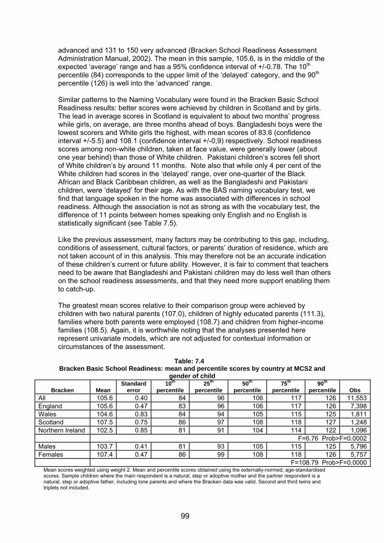
advanced and 131 to 150 very advanced (Bracken School Readiness Assessment Administration Manual, 2002). The mean in this sample, 105.6, is in the middle of the expected ‘average’ range and has a 95% confidence interval of +/-0.78. The 10th percentile (84) corresponds to the upper limit of the ‘delayed’ category, and the 90th percentile (126) is well into the ‘advanced’ range. Similar patterns to the Naming Vocabulary were found in the Bracken Basic School Readiness results: better scores were achieved by children in Scotland and by girls. The lead in average scores in Scotland is equivalent to about two months’ progress while girls, on average, are three months ahead of boys. Bangladeshi boys were the lowest scorers and White girls the highest, with mean scores of 83.6 (confidence interval +/-5.5) and 108.1 (confidence interval +/-0,9) respectively. School readiness scores among non-white children, taken at face value, were generally lower (about one year behind) than those of White children. Pakistani children’s scores fell short of White children’s by around 11 months. Note also that while only 4 per cent of the White children had scores in the ‘delayed’ range, over one-quarter of the Black African and Black Caribbean children, as well as the Bangladeshi and Pakistani children, were ‘delayed’ for their age. As with the BAS naming vocabulary test, we find that language spoken in the home was associated with differences in school readiness. Although the association is not as strong as with the vocabulary test, the difference of 11 points between homes speaking only English and no English is statistically significant (see Table 7.5). Like the previous assessment, many factors may be contributing to this gap, including, conditions of assessment, cultural factors, or parents’ duration of residence, which are not taken account of in this analysis. This may therefore not be an accurate indication of these children’s current or future ability. However, it is fair to comment that teachers need to be aware that Bangladeshi and Pakistani children may do less well than others on the school readiness assessments, and that they need more support enabling them to catch-up. The greatest mean scores relative to their comparison group were achieved by children with two natural parents (107.0), children of highly educated parents (111.3), families where both parents were employed (108.7) and children from higher-income families (108.5). Again, it is worthwhile noting that the analyses presented here represent univariate models, which are not adjusted for contextual information or circumstances of the assessment.
Table: 7.4 Bracken Basic School Readiness: mean and percentile scores by country at MCS2 and
gender of child
Bracken Mean Standard
error 10th
percentile 25th
percentile 50th
percentile 75th
percentile 90th
percentile
Obs All 105.6 0.40 84 96 106 117 126 11,553England 105.6 0.47 83 96 106 117 126 7,398Wales 104.6 0.83 84 94 105 115 125 1,811Scotland 107.5 0.75 86 97 108 118 127 1,248Northern Ireland 102.5 0.85 81 91 104 114 122 1,096 F=6.76 Prob>F=0.0002 Males 103.7 0.41 81 93 105 115 125 5,796Females 107.4 0.47 86 99 108 118 126 5,757 F=108.79 Prob>F=0.0000
Mean scores weighted using weight 2. Mean and percentile scores obtained using the externally-normed, age-standardised scores. Sample children where the main respondent is a natural, step or adoptive mother and the partner respondent is a natural, step or adoptive father, including lone parents and where the Bracken data was valid. Second and third twins and triplets not included.
99

Table: 7.5 Bracken Basic School Readiness: mean and percentile scores by child’s ethnicity and gender
Mean scores weighted using weight 2. Mean and percentile scores obtained using the externally-normed, age-standardised scores. Sample: children where the main respondent is a natural, step or adoptive mother and the partner respondent is a natural, step or adoptive father, including lone parents, where the Bracken and child’s ethnicity data were valid. Second and third twins and triplets not included.
Bracken Mean Standard
Error 10th
percentile 25th
percentile 50th
percentile 75th
percentile 90th
percentile
Obs White 106.2 0.41 85 96 107 117 126 9992Mixed background 104.8 1.25 81 93 106 116 126 322Black Caribbean 97.0 2.26 73 82 96 110 123 127Black African 96.3 1.92 71 83 94 111 123 164Bangladeshi 87.6 1.38 65 77 86 97 110 97Indian 102.9 1.96 79 89 102 117 127 270Pakistani 91.3 1.30 71 81 90 101 110 395Other background 103.7 2.13 75 87 107 117 127 143 F=44.31 Prob>F=0.0000White male 104.4 0.42 83 94 105 115 125 5036Mixed background male 104.0 1.68 81 93 105 117 126 156Black Caribbean male 93.6 2.80 73 79 88 107 127 66Black African male 91.8 2.79 68 75 91 104 115 77Bangladeshi male 83.6 2.81 65 73 83 94 99 37Indian male 101.9 2.14 77 88 102 116 125 132Pakistani male 88.7 1.30 71 79 88 96 105 192Other background male 103.6 2.90 75 86 107 117 131 76 F=35.26 Prob>F=0.0000White female 108.1 0.47 83 96 107 115 122 4956Mixed background female 105.7 1.57 82 94 107 116 129 166Black Caribbean female 100.5 2.50 81 88 101 112 119 61Black African female 100.1 2.37 75 86 99 118 125 87Bangladeshi female 90.1 1.33 71 77 88 101 111 60Indian female 103.7 2.41 79 91 103 118 128 138Pakistani female 94.0 2.01 72 83 93 103 121 203Other background female 103.8 2.66 77 89 104 115 125 67
F=33.54 Prob>F=0.0000 Language spoken in the home English only 106.09 0.4 84 93 103 110 120 10148English and other languages 100.6 1.15 77 84 95 105 118 1150No English spoken 94.601 2.95 67 75 88 95 115 255
F=14.37, Prob>F=0.000 (testing the three means) F=23.53, Prob>F=15.19 (testing mean1 and mean2)
100

Table: 7.6
Bracken Basic School Readiness: mean and percentile scores by family type, parental education, parental employment, NS-SEC status and equivalised family income at MCS2
Mean scores weighted using weight 2. Mean and percentile scores obtained using the externally-normed, age-standardised scores. Sample children where the main respondent is a natural, step or adoptive mother and the partner respondent is a natural, step or adoptive father, including lone parents, where valid Bracken test date data were available along with type, parental education, employment status, occupation or equivalised family income. Second and third twins and triplets not included. Notes: Parental qualifications and occupation relate to the higher of either of the parents in two-carer families or the highest qualification or occupation of lone parents. Equivalised income was calculated from grouped income data using a McClements-type equivalence scale (see chapter 10).
Bracken Mean Standard
error 10th
percentile 25th
percentile 50th
percentile 75th
percentile 90th
percentile
Obs Family structure Two natural parents 107.0 0.41 86 97 107 118 127 9,069Natural lone parent 99.4 0.49 79 88 100 110 120 2,276One natural and one step 98.3 1.33 77 87 102 108 117 193 F=161.07 Prob>F=0.0000Highest parental qualification NVQ5/NVQ4 111.3 0.47 93 103 112 121 129 4,187NVQ3 106.0 0.48 86 97 106 116 125 1,837NVQ2 102.1 0.43 83 91 103 112 121 2,173 NVQ1 97.7 0.92 77 86 98 110 117 395No qualifications 94.5 1.00 75 83 94 105 117 506 F=129.63 Prob>F=0.0000Earners in family Two people employed 108.7 0.38 89 100 109 119 127 5,206One person employed 105.4 0.53 84 95 106 116 126 4,194No one employed 96.1 0.54 75 84 96 107 117 2,153 F=314.71 Prob>F=0.0000Highest parental occupation Managerial/ professional 110.7 0.43 92 102 111 120 128 4,710Intermediate 106.7 0.57 87 98 107 116 125 1,167Small employer and self-employed 102.4 0.70 81 91 103 115 123 923Lower supervisors and technical 101.7 0.65 81 91 103 112 121 903Semi-routine and routine 98.4 0.58 79 86 99 108 118 1,497 F=126.67 Prob>F=0.0000Equivalised family income Above 60 percent median income 108.48 0.39 88 99 108 119 127 8,143Below 60 percent median income 97.57 0.44 77 86 97 108 118 3,630 F=715.20 Prob>F=0.0000
101

Behavioural adjustment Unlike the assessments of cognitive development which were directly measured from the child, indicators of behavioural adjustment are based on mothers’ reports. SDQ overall difficulty scores describing 12,018 children are given in table 7.7. The estimated raw mean score for total difficulties reported is 9.3 (95% confidence interval +/-0.16) and the range of the total difficulties score is between 0 and 40. Scores of between 14 and16 are classified as borderline and scores of 17 and above are classified as abnormal (Goodman 2001). An abnormal score could be reached in different ways, for example , if it was ‘somewhat true’ that the child had 17 out of 20 problems, ‘certainly true’ that they showed at least nine of them, or some intermediate combination. The raw mean score reported for the whole sample was 9.3, which falls into the normal range. Ten per cent of boys had scores in the abnormal range, 17 or above, whereas for girls, the worst 10 per cent mark was in the borderline category When comparing countries, Scotland and Northern Ireland have lower mean scores of 8.9 and 8.7 respectively, indicating significantly fewer behavioural problems in those countries on the four domains encompassed by the total difficulties score. Examining the different ethnic groups shows that mothers of Black African children report the least behaviour problems (i.e. lowest mean scores of 8.7 (confidence interval +/-0.8), followed by White children (mean score 9.2 +/-0.16). For all other ethnic groups we find scores higher than the sample mean, with Bangladeshi and Pakistani children obtaining scores of 12 and 13 respectively, indicating relatively increased behavioural problems (with confidence limits of 1.16 and 1.04 either side respectively). Black African girls have the lowest mean difficulties score (8.1) across all the groups split by gender and ethnicity; White, mixed background, Indian and other ethnic group females also have scores below the sample mean (8.7, 9.1, 8.5 and 9 respectively). For males, only Black African boys had scores below the overall sample average at 9.2. In interpreting these findings, it has to be kept in mind, that behavioural adjustment was assessed via parental report, and that there might be ethnic differences in reporting, parental language skills or item interpretation. The total difficulties score is higher for children in homes where no English is said to be spoken (10.87) compared to 9.24 in homes speaking only English. Children growing up in bilingual homes fall in between these two groups. All three groups are significantly different from one another.
Children described by their parent as having relatively low behavioural problems were those with two natural parents (8.9); those with more educated parents (9.1 for NVQ3 and 7.9 for NVQ4 or higher); or children in households where there were two employed adults (8.4). Children from higher socio-economic groups, where the mean score was 8.1 for children of managerial/professional parents, and those in higher income families, with mean scores of 7.5 and 8. 5 for the two highest household income groups, were also assessed as having lower difficulties scores.
At the problematic extreme, groups where as many as 10 per cent or more had an abnormal score above 17 were: boys, ethnic groups from South Asia, lone parents, step-families, parental occupation in the lower two classes, and adjusted family income below £330 per week.
102

Table: 7.7
Total Behaviour Difficulties Score: mean and percentiles by selected characteristics at MCS2 Total Difficulties Score Mean
Standard Error
10th per- centile
25th per-centile
50th per-centile
75th per-centile
90th per-centile Obs
All 9.3 0.08 3 5.5 9 12 16 12,018England 9.4 0.10 3 6 9 12 16 7,680Wales 9.1 0.14 3 5 8.3 12 16 1,865Scotland 8.9 0.18 3 5 8 12 15.8 1,390Northern Ireland 8.7 0.17 3 5 8 12 16 1,083
F=4.79 Prob>F=0.0027Child gender Males 9.8 0.09 4 6 9 13 17 6,120Females 8.8 0.1 3 5 8 12 15.8 5,898
F=97.18 Prob>F=0.0000Ethnic group White 9.2 0.08 3 5.3 8.5 12 16 10,467Mixed background 9.4 0.31 3 6 9 12.3 16.5 352Black Caribbean 9.9 0.53 4 6.3 10 13 16.3 149Black African 8.7 0.41 2 5 8.5 11.3 14.8 174Bangladeshi 12 0.59 5 8 10.3 16 19.3 98Indian 9.7 0.49 3 5.3 9 13 17 260Pakistani 13 0.53 5 8 10.3 16 19.3 329Other background 10.2 0.75 3 5.3 9 14 20 153
F=11.66 Prob>F=0.0000Ethnic group Boys White male 9.7 0.1 4 6 9 13 17 5,347Mixed background male 9.8 0.43 3 6 9 13 16.8 170Black Caribbean male 10.3 0.63 4 6.8 10 13 16 78Black African male 9.2 0.63 2 6 9 12.3 14.8 88Bangladeshi male 12 1.22 5 7.3 10 15.8 24 45Indian male 10.8 0.61 4 6 10 14.8 18.8 138Pakistani male 13.6 0.6 5.6 8.8 12.7 18 22.8 155Other background male 11.4 1.1 3 6 10 15.8 23 79
F=8.31 Prob>F=0.0000Ethnic group Girls White female 8.7 0.1 3 5 8 11.7 15.3 5,120Mixed background female 9.1 0.43 3 6 8 11.8 16 182Black Caribbean female 9.4 0.67 5 6 10 12 16.3 71Black African female 8.1 0.52 3 5 7.5 10.4 14.7 86Bangladeshi female 12 0.78 7 8.7 11 16.8 19 53Indian female 8.5 0.57 3 4.5 7.8 11 16 122Pakistani female 12.5 0.73 6 8 11.7 17 22 174
103

Table: 7.7 Total Behaviour Difficulties Score: mean and percentiles by selected characteristics at MCS2
Total Difficulties Score Mean
Standard Error
10th per- centile
25th per-centile
50th per-centile
75th per-centile
90th per-centile Obs
Other background female 9 0.71 3 5 8 12 16 74
F=6.98 Prob>F=0.0000Contd. Language spoken in the home
English only 0.84
3.00
5.00
7.00
10.00
14.00 9.24 10,665English and other languages
3.00
5.00
7.50
11.00 9.97 0.32
15.00 1,145
No English spoken 10.87 0.62
5.00
5.40
8.00
11.00
16.67 208F=5.87, prob>F=0.0031 (testing the three means)
F=5.31, prob>F=0.0217 (testing mean1 and mean2) Family structure
Two natural parents 8.9 0.07 3 5 8 12 15.5 9,386Natural lone parent 11.2 0.16 4 7 10.5 15 19.3 2414One natural and one step-parent 11.8 0.45 5 8 11.8 15 20.5 204
F=131.31 Prob>F=0.0000Highest parental education NVQ5/NVQ4 7.9 0.09 3 5 7 10.5 14 4,370NVQ3 9.1 0.13 3.8 6 8.3 12 15.8 1,932NVQ2 10.2 0.12 4 6.3 9.6 13 17 2,270NVQ1 11.1 0.35 4 6.5 10.3 15 19 394No qualifications 11.9 0.32 5 7 11 16 20 468
F=99.29 Prob>F=0.0000Highest parental occupation Managerial/ professional 8 0.08 3 5 7 11 14 4,949Intermediate 9.1 0.16 3.5 5.7 9 12 15 1,223Small employer & self-employed 9.3 0.2 3.3 6 8.7 12.1 16 913Lower supervisor & technical 10.4 0.19 4 6.7 9.5 13.8 17.3 932Semi-routine & routine 11.4 0.17 5 7 11 15 19 1,518
F=87.87 Prob>F=0.0000 Equivalised family income Above 60 percent median income 8.6 0.07 3 5 8 11 15 8,588Below 60 percent median income 11.4 0.13 5 7 11 15 19 3,761 F=596.54 Prob>F=0.000
Mean scores weighted using weight 2. Sample children where the main respondent is a natural, step or adoptive mother and the partner respondent is a natural, step or adoptive father, including lone parents. Second and third twins and triplets not included. Note: Analysis by ethnicity uses the child’s ethnicity; parental qualifications and occupation relating to the higher of either of the parents in two- carer families or the highest qualification or occupation of lone parents.
104

Language in Wales The foregoing analysis of homes where languages other than English is spoken at the UK level did not take into account that in Wales there are two official languages. The general implication of an association of not speaking English with delayed development, particularly in vocabulary, but also emotional adjustment may not apply in this situation. About one-tenth of respondents in Wales reported speaking some or only Welsh at home. A small number of families opted to do the child assessment or adult interviews in Welsh (see Moon, 2006), but there were also assessments done in English on 175 families. These results are almost the reverse of the general picture. Children in those Welsh homes where any Welsh was reported as being spoken had an almost identical distribution of scores at age 3 on both the Vocabulary and School Readiness Scores as other children in Wales speaking only English. If anything, the average cognitive scores were higher in the Welsh-speaking homes, but not significantly so. There were fewer children with high problem behaviour scores in the Welsh-speaking homes than those in Wales where only English was spoken (the mean behaviour problem scores were 7.92 and 9.23 respectively, a modest but statistically significant difference). Neither set of results proves that a bilingual upbringing is either an asset or a handicap as far as developmental assessments go, although to be acquiring a second language is an asset in itself. It may also play a part among other factors, and signal other differences between families which need to be considered with multivariate methods.
Looking back at earlier developmental milestones We now compare indicators of development at age three with the developmental milestones measured in the first MCS survey: gross motor functions, fine motor functions and communicative gestures. Gross motor skills include standing and walking, while examples of fine motor skills are being able to pick up small objects. To make communicative gestures at nine months, includes smiling and waving goodbye. Delays are identified for, by definition, a minority who have not reached the stage normal for their age (Schoon et al 2005).Children classified as having one or more delays at age nine months on average achieved worse scores in all the three assessments at three years of age.
The mean BAS vocabulary score for the whole sample is 50.6; similar mean scores were achieved by children without any developmental delays. However, the minority of children who had had one or more gross motor function delays had a mean score of 48. Those with one or more fine motor function delays at nine months had a mean score of 48.3 and those with one or more delay in communicative gestures at the earlier stage achieved a mean score of 48.4 (all still within the ‘average’ range). The mean Bracken score for the whole sample was 105.6, and again children without any delays at nine months achieved comparable mean scores. Children who had had gross motor function delays had a mean score of 101.9. Those with earlier fine motor function delays had scores of 102.3 and those with previous delays in communicative
105

gestures had a mean score of 101.5. Again, this is still within the ‘average’ range, but lower. The total behaviour difficulties scores show the same pattern: children with one or more delays at nine months in any of the three developmental milestones obtained worse mean scores than the overall sample and than those without any delays. Children displaying developmental delays in communicative gestures at nine months have the highest mean problem score at age three (10.8). These differences are all statistically significant and suggest that not all early delays are compensated for by subsequent catch-up. The indicators of developmental milestones at nine months, especially communicative gestures, did not appear to be as clearly socially patterned as socio-emotional adjustment measured at three. This could be because behavioural problems in babies are less clearly measured, or because socially divergent patterns emerge as a baby grows into a three-year-old.
Table: 7.8 BAS Naming Vocabulary: mean and percentile scores at age three by developmental milestone
measures at nine months
BAS Mean Standard
error 10th
percentile 25th
percentile 50th
percentile 75th
percentile 90th
percentile
Obs All 50.6 0.21 38 43 49 58 67 12,096No gross motor function delays at nine months 51.1 0.20 38 44 50 58 67 10,387 One or more gross motor function delays at nine months 48.0 0.40 34 41 47 56 63 1,709 F=80.85 Prob>F=0.0000No fine motor function delays at nine months 50.9 0.21 38 43 50 58 67 10,906 One or more fine motor function delays at nine months 48.3 0.39 36 41 48 56 63 1,190 F=54.69 Prob>F=0.0000No communicative gesture delays at nine months 50.7 0.21 38 43 49 58 65 11,550 One or more communicative gesture delays at nine months 48.4 0.60 34 41 49 56 63 546 F=18.06 Prob>F=0.0000
Mean scores weighted using weight 2. Sample: children where the main respondent is a natural, step or adoptive mother and the partner respondent is a natural, step or adoptive father, including lone parents, where BAS scores and developmental milestone measures have been specified. Second and third twins and triplets not included.
106

Table: 7.9 Bracken School Readiness: mean and percentile scores at age three by developmental milestone
measures at nine months
Bracken Mean Standard
error 10th
percentile 25th
percentile 50th
percentile 75th
percentile 90th
percentile
Obs All 105.6 0.40 84 96 106 117 126 11,533No gross motor function delays 106.2 0.40 84 96 107 117 126 9,938One or more gross motor function delays 101.9 0.67 79 89 102 115 124 1,615 F=64.13 Prob>F=0.0000No fine motor function delays 106.0 0.40 84 96 107 117 126 10,417One or more fine motor function delays 102.3 0.67 79 90 103 115 125 1,136 F=42.74 Prob>F=0.0000No communicative gesture delays 105.8 0.40 84 96 106 117 126 11,030One or more communicative gesture delays 101.5 0.88 79 89 102 114 124 523 F=31.31 Prob>F=0.0003
Mean scores weighted using weight 2. Sample children where the main respondent is a natural, step or adoptive mother and the partner respondent is a natural, step or adoptive father, including lone parents, where Bracken scores and developmental milestone measures have been specified. Second and third children in twins and triplets not included.
Table: 7.10
Total Behavioural Difficulties: mean and percentile scores at age three by developmental milestone measures at nine months
Total Difficulties Score Mean
Standard Error
10th percentile
25th percentile
50th percentile
75th percentile
90th percentile
Obs
All 9.3 0.08 3.0 5.5 9.0 12.0 16.0 12,018No gross motor function delays at nine months 9.2 0.08 3.0 5.3 8.3 12.0 16.0 10,329One or more gross motor function delays at nine months 10.2 0.19 4.0 6.0 9.2 13.8 18.0 1,689 F=37.46 Prob>F=0.0000No fine motor function delays at nine months 9.2 0.08 3.0 5.3 8.3 12.0 16.0 10,836One or more fine motor function delays at nine months 10.6 0.21 4.0 6.0 10.0 14.0 18.3 1,182 F=55.28 Prob>F=0.0000No communicative gesture delays at nine months 9.2 0.08 3.0 5.5 8.8 12.0 16.0 11493One or more communicative gesture delays at nine months 10.8 0.30 4.0 6.0 10 14.0 18.5 525 F=30.01 Prob>F=0.0028
Mean scores weighted using weight 2. Sample children where the main respondent is a natural, step or adoptive mother and the partner respondent is a natural, step or adoptive father, including lone parents, where a total difficulties scores and developmental milestone measures have been specified. Second and third twins and triplets not included.
107

Conclusion This chapter has provided an overview of child outcomes at age three using cognitive and behavioural assessments. The scores for the sample fell as much within and outside the normal range for all three assessments as would be expected for children of their age. However, the results showed a marked difference in children from advantaged versus disadvantaged backgrounds, exemplified by the better scores achieved by children from families with two working parents, high family incomes and highly educated parents. All three assessments show that a picture of early childhood disadvantage is emerging as likely to have important implications for educational progress and adjustments in later life. There also appear to be substantial differences between ethnic groups, with Bangladeshi and Pakistani children showing signs of slower cognitive development and lower parent reported behavioural adjustment. However, as already noted, a range of other factors which have not been taken into account in this analysis could account, partially or even fully, for these ethnic differences. Data on minority groups are subject to greater sampling error than larger groups, and may be particularly variable as concerns members of ethnic groups who do not live in the over sampled areas of concentrated minority ethnic settlement, or among ethnic minority children born into different social strata. The response rates of some non-White groups, cultural expectations, the importance of other languages being spoken at home, and number of siblings are just some of the factors that warrant further investigation. There is also scope for further investigation of differences in the development scores in the separate countries of the UK, and in particular of the role of bilingualism in Wales. References Bracken, B. A. (1998). Bracken. Basic Concept Scale - Revised. San Antonio, Texas: The Psychological Corporation.
Bracken, B. A. (2002). Bracken School Readiness Assessment Administration Manual. San Antonio, TX: The Psychological Corporation.
Bricker, D., Squires, J., Mounts, L., Potter, L., Nickel, B., & Farrell, J. (1995). Ages and Stages Questionnaire. Baltimore: Paul H. Brookes.
Elliott, C. D. (1983). British Ability Scales. Windsor, UK: NFER-Nelson.
Elliott, C.D., Smith, P. & McCulloch, K. (1997) British Abilities Scale II Technical Manual. London, UK: NFER-Nelson.
Fenson, L., Dale, P. S., Resnick, J. S., Thal, D., Bates, E., Hartung, J. P., et al. (1993). MacArthur Communicative Development Inventories (CDI). San Diego, CA: Singular Publishing Group.
Frankenburg, W. K., & Dodds, J. B. (1967). Denver Developmental Screening Test J. Paediatrics, 71, 181-191.
Frankenburg, W. K., & Dodds, J. B. (1990). Denver II screening manual. Denver, CO: Denver Developmental Materials.
Goodman, R. (1997). The Strengths and Difficulties Questionnaire: A Research Note
Journal of Child Psychology and Psychiatry, 38, 581-586.
108

Goodman, R. (2001). Psychometric properties of the Strengths and Difficulties Questionnaire (SDQ) Journal of the American Academy of Child and Adolescent Psychiatry, 40(1337-1345).
Goodman, R., Meltzer, H., & Bailey, V. (1998). The Strengths and Difficulties Questionnaire: A pilot study on the validity of the self-report version, European Child and Adolescent Psychiatry, 7, 125-130.
Moon, N. (2006) Technical Report on Fieldwork, London: NOP. http://www.cls.ioe.ac.uk/studies.asp?section=00010002000100040006
Schoon, I., Sacker, A., Hope, S., Collishaw, S., & Maughan, B. (2005). Children’s development in the family environment. In S. Dex & H. Joshi (Eds.), Babies of the New Millennium (pp. 159-174): Polity Press
109

Chapter 8 PARENTAL HEALTH AND WELLBEING Lisa Calderwood, Yvonne Kelly and Lidia Panico Introduction The health of parents matters in our account of the Millennium Cohort Study, as it forms an important part of the context in which children grow up. The second sweep of the MCS collected data on health and related behaviours including general self-rated health, longstanding illnesses, psychological morbidity, smoking, alcohol and other drug use, and height and weight. Each of these is considered for mothers and fathers in relation to age, country of residence, ethnicity, occupation, educational qualifications, family structure and employment status. Health and longstanding illness Self-rated health Parents were asked to describe their health as ‘excellent’, ‘good’, ‘fair’ or ‘poor’. Overall, about 31 per cent of mothers rated it ‘excellent’, 51 per cent ‘good’, 15 per cent ‘fair’ and 3 per cent ‘poor’. Slightly higher proportions of fathers rated their health ‘excellent’ (35 per cent) and ‘good’ (52 per cent), with lower proportions of fathers rating it ‘fair’ (12 per cent) and poor (2 per cent). Fair/poor health was reported by one in six mothers (Table 8.1). This varied by occupation, highest educational qualification, ethnic group, age, employment status and family composition. For example, mothers in less skilled occupations were twice as likely to have fair/poor health as the most skilled. Indian, Pakistani, Bangladeshi and Black Caribbean mothers were more likely to report fair/poor health compared with White mothers. Mothers in England were the most likely (17.7 per cent) to report fair or poor health and those in Scotland and Northern Ireland were the least likely (15.1 per cent and 15.6 per cent). These differences were statistically significant at the 6 per cent level. About one in seven fathers reported fair/poor health and similar variations to those seen in mothers were observed. Country differences were not statistically significant.
Table 8.1 Parents’ general health at sweep 2
Total Percentage fair or poor health
Mothers Total (all who completed main interview) 15,229 17.4Age Under 25 2,151 24.5 25 to 29 2,997 22.0 30 to 34 4,823 14.9 35 to 39 3,875 14.3 40 and over 1,372 18.3
110

Table 8.1 Parents’ general health at sweep 2
Total Percentage fair or poor health
Contd. p value
Chi square 0.0000 152.78
Country England 9,810 17.7 Wales 2,200 16.5 Scotland 1,785 15.1 N. Ireland 1,434 15.6 p value
Chi square 0.0519
10.89 Ethnicity White 12,473 16.5 Mixed 128 17.3 Indian 366 19.4 Pakistani 652 28.8 Bangladeshi 247 25.7 Black Caribbean 178 25.8 Black African 240 18.8 Other ethnicity 257 20.0 p value
Chi square 0.0000
56.27 Occupational class Managerial and professional 2,866 9.6 Intermediate 1,848 11.9 Small employer and self-employed 522 11.4 Lower supervisory and technical 311 19.3 Routine and semi-routine 2,100 18.1 p value
Chi square 0.0000
88.94 Couples’ employment Both partners employed 6,669 11.9 Main employed, partner not employed 308 20.9 Partner employed, main not employed 4,647 18.5 Neither employed 969 36.8 p value
Chi square 0.0000 343.41
Education level NVQ 1 1,234 23.3 NVQ 2 4,314 18.9 NVQ 3 2,226 15.8 NVQ 4 4,304 11.5 NVQ 5 582 9.3 Other/overseas qualifications 477 27.6 None of the above 2,060 30.9 p value
Chi square 0.0000 404.24
Family type Married natural parents 9,384 14.0 Cohabiting natural parents 2,339 21.4 Natural parents (other/unknown
relationship) 563 19.2 Lone natural mother 2,575 25.9
Other 368 27.7 p value
Chi square 0.0000 244.24
Fathers Total (all fathers who completed partner interview) 10,256 14.0Age Under 25 387 21.5 25 to 29 1,295 18.9
111

Table 8.1 Parents’ general health at sweep 2
Total Percentage fair or poor health
Contd. 30 to 34 2,953 13.6 35 to 39 3,291 11.2 40 and over 2,278 15.0 p value
Chi square 0.0000 61.75
Country England 6,707 14.1 Wales 1,488 12.1 Scotland 1,169 13.5 N. Ireland 892 13.3 p value
Chi square 0.29 4.39
Ethnicity White 8,114 13.6 Mixed 64 14.8 Indian 268 18.5 Pakistani 350 20.0 Bangladeshi 107 29.4 Black Caribbean 82 11.7 Black African 103 9.3 Other ethnicity 182 14.2 p value
Chi square 0.0029 21.48
Occupational class Managerial and professional 3,928 9.1 Intermediate 763 12.5 Small employer and self-employed 1,495 13.8 Lower supervisory and technical 1,420 19.7 Routine and semi-routine 2,575 20.8 p value
Chi square 0.0000 207.52
Couples’ employment Both partners employed 5,610 10.9 Main employed, partner not employed 258 33.6 Partner employed, main not employed 3,586 13.2 Neither employed 752 43.7 p value
Chi square 0.0000 523.99
Education level NVQ 1 646 22.1 NVQ 2 2,628 16.2 NVQ 3 1,462 12.1 NVQ 4 2,988 8.7 NVQ 5 622 5.4 Other/overseas qualifications 398 21.1 None of the above 1,106 27.9 p value
Chi square 0.0000 315.77
Family type Married natural parents 7,675 12.4 Cohabiting natural parents 1,852 19.4 Natural parents (other/unknown
relationship) 504 13.9 Other 225 26.9 p value 0.0000
Chi square 86.98 Note: Total bases are unweighted. Percentages are weighted. Variable used for weighting: weight 2, apart from analysis by country which uses weight 1. Lone fathers not included.
112

Longstanding illness Such illness is defined as ‘a longstanding illness, disability or infirmity that has troubled you over a period of time or is likely to affect you over a period of time’. About one in five parents reported such illness (Table 8.2), although it is not known how many had to limit their activities as a result.
Table 8.2 Parental longstanding illness at sweep 2
Total Percentage longstanding illness
Mothers Total (all who completed main interview) 15,229 21.4Age Under 25 2,151 21.8 25 to 29 2,997 23.1 30 to 34 4,823 20.1 35 to 39 3,875 20.9 40 and over 1,372 23.6 p value
Chi square 0.02
14.35 Country England 9,810 21.3 Wales 2,200 22.8 Scotland 1,785 22.7 N. Ireland 1,434 19.4 p value
Chi square 0.11 8.61
Ethnicity White 12,473 21.7 Mixed 128 23.1 Indian 366 18.2 Pakistani 652 13.8 Bangladeshi 247 18.4 Black Caribbean 178 24.2 Black African 240 12.0 Other ethnicity 257 17.5 p value
Chi square 0.0003
27.60 Occupational class Managerial and professional 2,866 17.9 Intermediate 1,848 17.3 Small employer and self-employed 522 22.9 Lower supervisory and technical 311 22.2 Routine and semi-routine 2,100 19.6 p value
Chi square 0.0171
14.26 Couples’ employment Both partners employed 6,669 18.4 Main employed, partner not
employed 308 23.2 Partner employed, main not
employed 4,647 21.8 Neither employed 969 33.3 p value
Chi square 0.0000
95.06 Education level NVQ 1 1,234 22.9 NVQ 2 4,314 23.6 NVQ 3 2,226 19.5 NVQ 4 4,304 19.6 NVQ 5 582 16.3
113

Table 8.2 Parental longstanding illness at sweep 2
Total Percentage longstanding illness
Contd. Other/overseas qualifications 477 20.3 None of the above 2,060 24.5 p value
Chi square 0.0000
47.40 Family type Married natural parents 9,384 19.6 Cohabiting natural parents 2,339 23.5 Natural parents (other/unknown
relationship) 563 21.4 Lone natural mother 2,575 25.7 Other 368 30.4 p value
Chi square 0.0000
66.36 Fathers Total (all who completed partner interview) 10,256 21.2Age Under 25 387 22.7 25 to 29 1,295 20.7 30 to 34 2,953 19.0 35 to 39 3,291 19.6 40 and over 2,278 25.8 p value
Chi square 0.0000
44.07 Country England 6,707 21.3 Wales 1,488 22.1 Scotland 1,169 20.7 N. Ireland 892 16.8 p value
Chi square 0.037 12.17
Ethnicity White 8,114 21.8 Mixed 64 24.4 Indian 268 18.8 Pakistani 350 17.3 Bangladeshi 107 18.0 Black Caribbean 82 18.1 Black African 103 15.6 Other ethnicity 182 15.6 p value
Chi square 0.25
9.0005 Occupational class Managerial and professional 3,928 19.2 Intermediate 763 24.1 Small employer and self-employed 1,495 18.6 Lower supervisory and technical 1,420 24.4 Routine and semi-routine 2,575 23.8 p value
Chi square 0.0000
37.02 Couples’ employment Both partners employed 5,610 19.2 Main employed, partner not
employed 258 38.8 Partner employed, main not
employed 3,586 19.0 Neither employed 752 47.4 p value 0.0000
Chi square 291.87
114

115
Table 8.2 Parental longstanding illness at sweep 2
Total Percentage longstanding illness
Contd. Education level NVQ 1 646 22.2 NVQ 2 2,628 22.3 NVQ 3 1,462 19.5 NVQ 4 2,988 20.5 NVQ 5 622 16.1 Other/overseas qualifications 398 25.0 None of the above 1,106 26.0 p value
Chi square 0.0014
30.21 Family type Married natural parents 7,675 20.3 Cohabiting natural parents 1,852 23.8 Natural parents (other/unknown
relationship) 504 23.4 Other 225 28.3 p value
Chi square 0.0030
18.68 Note: Total bases are unweighted. Percentages are weighted. Variable used for weighting: weight 2, , apart from analysis by country which uses weight 1. Lone fathers not included. .
Health-related behaviour Cigarette smoking About three in 10 mothers were smokers, varying by age, ethnic group, occupation, educational qualifications and family composition (Table 8.3). The likelihood of smoking decreases with age, with more than half of younger mothers (under 25) smoking at the time of interview compared with about one in five of those aged 35 or above. Younger mothers were also most likely to smoke heavily, with one in 10 smoking 20 or more cigarettes per day. Indian, Pakistani, Bangladeshi and Black African mothers were less likely to smoke than White mothers. Black Caribbean mothers were most likely to smoke, though White mothers were most likely to be heavy smokers. Mothers in the most skilled occupations were less likely to smoke and be heavy smokers than those less skilled. Lone mothers were more likely to smoke and be heavy smokers than mothers in married two-parent families, although there was no difference between lone mothers and those in co-habiting households. Similar patterns by age, occupation and educational level were seen for fathers, with the exception of ethnic group: Pakistani and Bangladeshi fathers were more likely to smoke than White fathers, though less likely to be such heavy smokers.

Table 8.3
Parental smoking status at sweep 2 Total
Non-smoker Under 10
cigarettes (inc. roll-ups)
10-19 cigarettes (inc. roll-ups)
20+ cigarettes (inc. roll-ups)
Other tobacco products
Per cent Per cent Per cent Per cent Per cent Mothers Total (all who completed main interview) 15,229 72.5 9.2 12.2 6.0 0.1 Age Under 25 2,151 45.8 15.8 27.9 10.4 0.0 25 to 29 2,997 62.1 13.8 16.2 7.8 0.1 30 to 34 4,823 76.4 7.8 10.2 5.5 0.1 35 to 39 3,875 82.4 6.5 7.0 4.0 0.1 40 and over 1,372 82.2 5.2 7.4 5.2 0.1 p value
Chi square 0.0000
1166.55
Country England 9,810 73.1 9.1 12.0 5.8 0.1 Wales 2,200 67.4 11.0 13.7 7.8 0.0 Scotland 1,785 71.1 8.7 13.5 6.5 0.2 N. Ireland 1,434 71.4 7.4 12.9 8.2 p value
Chi square 0.0005
56.64
Ethnicity White 12,473 71.6 9.3 12.7 6.4 0.0 Mixed 128 64.7 18.0 12.8 4.5 Indian 366 92.7 2.9 3.1 0.7 0.6 Pakistani 652 95.2 4.0 0.6 0.1 0.1 Bangladeshi 247 98.1 1.3 0.5 Black Caribbean 178 62.9 22.8 10.9 1.6 1.8 Black African 240 89.6 6.9 3.6 Other ethnicity 257 88.5 6.6 3.0 1.6 0.4 p value
Chi square 0.0000376.07
Occupational class Managerial and professional 2,866 86.8 6.3 5.0 1.8 0.1 Intermediate 1,848 80.4 9.7 7.4 2.5 0.1 Small employer and self-
employed 522 81.5 6.8 8.6 3.1 Lower supervisory and technical 311 65.1 14.7 13.6 6.7 Routine and semi-routine 2,100 64.1 11.8 16.9 7.2 p value
Chi square 0.0000 443.65
116

Table 8.3
Total Parental smoking status at sweep 2
Non-smoker
10-19 cigarettes (inc. roll-ups)
20+ cigarettes (inc. roll-ups)
Other tobacco products
Under 10 cigarettes (inc. roll-
ups) Per cent Per cent Per cent Per cent Per cent Contd. Couples’ employment Both partners employed 6,669 81.4 7.8 7.9 2.8 0.0 Main employed, partner not
employed 308 62.5 11.9 17.7 7.9 Partner employed, main not
employed 4,647 75.9 7.8 10.4 5.8 0.1 Neither employed 969 52.0 9.6 21.7 16.6 0.2 p value
Chi square 0.0000522.24
Education level NVQ 1 1,234 53.1 11.9 23.5 11.5 0.1 NVQ 2 4,314 65.6 11.3 16.2 6.8 0.1 NVQ 3 2,226 73.3 11.4 10.9 4.3 0.0 NVQ 4 4,304 87.1 6.3 4.5 2.0 0.0 NVQ 5 582 92.9 4.3 1.7 1.1 Other/overseas qualifications 477 76.2 5.9 9.7 7.9 0.3 None of the above 2,060 50.1 10.0 23.7 16.1 0.1 p value
Chi square 0.0000
1618.38
Family type Married natural parents 9,384 83.3 6.7 6.9 3.0 0.0 Cohabiting natural parents 2,339 56.2 13.3 20.1 10.3 0.1 Natural parents (other/unknown
relationship) 563 77.1 6.7 10.0 5.9 0.2 Lone natural mother 2,575 44.9 15.8 25.9 13.2 0.2 Other 368 49.9 10.9 24.6 14.6 p value
Chi square 0.0000
1924.50
Fathers Total (all who completed partner interview) 10,256 69.6 8.1 12.1 8.8 1.4 Age Under 25 387 41.2 14.0 31.2 13.5 25 to 29 1,295 51.5 14.1 21.3 12.7 0.4 30 to 34 2,953 68.9 7.8 13.4 8.6 1.4 35 to 39 3,291 75.6 7.9 8.0 7.2 1.3 40 and over 2,278 73.9 5.5 9.6 8.7 2.3
117

Table 8.3
Total Parental smoking status at sweep 2
Non-smoker
10-19 cigarettes (inc. roll-ups)
20+ cigarettes (inc. roll-ups)
Other tobacco products
Under 10 cigarettes (inc. roll-
ups) Per cent Per cent Per cent Per cent Per cent Contd. p value
Chi square 0.0000498.88
Country England 6,707 69.6 8.5 11.8 8.7 1.4 Wales 1,488 69.9 7.3 12.8 8.6 1.4 Scotland 1,169 69.5 6.3 14.0 8.9 1.3 N. Ireland 892 74.8 3.1 10.3 10.9 0.9 p value
Chi square 0.0002
54.53
Ethnicity White 8,114 70.4 7.4 11.7 8.9 1.5 Mixed 64 61.3 16.3 13.0 9.5 Indian 268 78.5 10.6 7.2 2.9 0.9 Pakistani 350 59.2 18.0 18.8 4.0 Bangladeshi 107 60.3 17.7 17.8 4.2 Black Caribbean 82 61.7 20.9 8.7 2.5 6.2 Black African 103 93.2 5.9 0.9 Other ethnicity 182 69.0 13.4 9.6 7.7 0.2 p value
Chi square 0.0001141.02
Occupational class Managerial and professional 3,928 80.2 6.5 7.5 4.1 1.8 Intermediate 763 79.5 7.9 7.2 4.1 1.3 Small employer and self-
employed 1,495 63.8 10.0 12.5 12.3 1.4 Lower supervisory and technical 1,420 60.7 8.6 16.1 13.1 1.5 Routine and semi-routine 2,575 53.4 10.1 21.0 14.8 0.6 p value
Chi square 0.0000751.44
Couples’ employment Both partners employed 5,610 74.4 7.6 10.1 6.4 1.4 Main employed, partner not
employed 258 51.0 14.3 21.4 13.2 0.1 Partner employed, main not
employed 3,586 68.2 8.2 12.4 9.6 1.6 Neither employed 752 36.9 10.9 25.7 26.3 0.2
118

119
Table 8.3
Total Parental smoking status at sweep 2
Non-smoker
10-19 cigarettes (inc. roll-ups)
20+ cigarettes (inc. roll-ups)
Other tobacco products
Under 10 cigarettes (inc. roll-
ups) Per cent Per cent Per cent Per cent Per cent Contd. p value
Chi square 0.0000499.02
Education level NVQ 1 646 55.0 7.9 19.8 16.0 1.3 NVQ 2 2,628 64.0 8.6 15.0 11.0 1.4 NVQ 3 1,462 68.9 8.0 12.3 8.7 2.1 NVQ 4 2,988 80.9 7.4 7.0 3.3 1.3 NVQ 5 622 88.0 6.4 2.0 1.8 1.8 Other/overseas qualifications 398 59.0 10.7 17.1 12.6 0.6 None of the above 1,106 48.5 9.7 20.3 20.7 0.8 p value
Chi square 0.0000781.19
Family type Married natural parents 7,675 74.5 7.3 9.6 7.0 1.5 Cohabiting natural parents 1,852 50.3 11.8 21.9 14.9 1.1 Natural parents (other/unknown
relationship) 504 68.6 7.9 12.4 10.0 1.2 Other 225 49.7 7.9 21.9 19.6 0.9 p value
Chi square 0.0000497.13
Note: Total bases are unweighted. Percentages are weighted. Variable used for weighting: weight 2, apart from analysis by country which uses weight 1. Lone fathers not included. .

120
Alcohol and problem drinking Frequency of alcohol consumption for mothers and fathers is shown in Table 8.4 and showed variations by age, country, ethnic group, occupation and education. For mothers, the likelihood of ever drinking alcohol rose with age. Those in Wales and Scotland were more likely to drink alcohol than mothers in England and Northern Ireland. Mothers from England and Wales, however, were most likely to drink alcohol five or more times per week (8 per cent and 7 per cent respectively) compared with those in Scotland and Northern Ireland (4 per cent and 1 per cent). Pakistani and Bangladeshi mothers were least likely (3 and 1 per cent respectively), and White and Black Caribbean mothers most likely, to drink any alcohol (88 and 80 per cent). Mothers in the most skilled occupations were more likely to drink alcohol five or more times per week than those in the least skilled occupations (11 and 5 per cent respectively). A similar pattern was seen across educational groups. Fathers in England and Wales were most likely to drink alcohol five or more times per week (17 and 15 per cent respectively) compared with those in Scotland and Northern Ireland (10 and 4 per cent). White and Black Caribbean fathers were most likely (95 and 85 per cent) and Bangladeshi and Pakistani fathers least likely (2 and 8 per cent) to ever drink alcohol.

Table 8.4
Frequency of parental drinking at sweep 2 Total Current alcohol use Never Less than
monthly Monthly Four times a
week or less Five or more times a week
Per cent Per cent Per cent Per cent Per cent Mothers Total (all who completed main interview) 15,229 17.3 18.5 18.2 38.7 7.4 Age Under 25 2,151 21.2 24.5 25.0 28.0 1.3 25 to 29 2,997 24.7 20.7 20.2 31.4 2.9 30 to 34 4,823 16.5 18.1 19.1 40.3 6.0 35 to 39 3,875 13.5 15.6 15.1 43.9 11.9 40 and over 1,372 13.0 16.4 12.0 44.3 14.3 p value
Chi square 0.0000 858.06
Country England 9,810 18.0 18.3 17.6 38.2 8.0 Wales 2,200 13.3 18.2 19.6 42.2 6.8 Scotland 1,785 12.0 20.0 22.1 42.0 3.9 N. Ireland 1,434 17.0 21.8 21.2 38.9 1.2 p value
Chi square 0.0000 217.60
Ethnicity White 12,473 11.8 19.0 19.1 42.0 8.1 Mixed 128 34.9 13.3 19.0 29.3 3.6 Indian 366 58.6 20.2 10.1 10.3 0.7 Pakistani 652 96.6 1.2 0.9 0.6 0.6 Bangladeshi 247 98.9 0.8 0.3 Black Caribbean 178 20.1 29.8 17.9 29.6 2.6 Black African 240 61.8 18.0 10.2 10.0 Other ethnicity 257 51.9 16.2 9.7 20.9 1.3 p value
Chi square 0.0000
3341.48 Occupational class Managerial and professional 2,866 9.2 13.7 17.3 48.9 10.9 Intermediate 1,848 11.2 19.5 20.2 43.7 5.5 Small employer and self-employed 522 11.5 14.1 15.9 46.6 12.0 Lower supervisory and technical 311 10.1 22.9 24.8 36.8 5.3 Routine and semi-routine 2,100 13.6 22.1 21.7 38.0 4.5 p value
Chi square 0.0000 228.08
121

Table 8.4
Frequency of parental drinking at sweep 2 Total Current alcohol use Never Less than
monthly Monthly Four times a
week or less Five or more times a week
Per cent Per cent Per cent Per cent Per cent Contd. Couples’ employment Both partners employed 6,669 10.7 17.4 19.1 44.5 8.3 Main employed, partner not employed 308 18.7 18.6 20.5 37.5 4.7 Partner employed, main not employed 4,647 22.9 18.4 15.5 35.1 8.1 Neither employed 969 39.8 20.8 12.7 22.5 4.1 p value
Chi square 0.0000 649.37
Education level NVQ 1 1,234 19.9 25.5 21.1 29.5 4.0 NVQ 2 4,314 14.4 22.0 19.9 38.4 5.3 NVQ 3 2,226 16.3 18.1 21.1 37.4 7.1 NVQ 4 4,304 11.6 14.3 16.8 46.5 10.8 NVQ 5 582 14.3 10.2 12.3 49.5 13.6 Other/overseas qualifications 477 50.6 16.4 11.8 16.9 4.2 None of the above 2,060 36.9 20.6 15.2 24.3 3.1 p value
Chi square 0.0000
1326.09 Family type Married natural parents 9,384 17.7 16.6 16.8 40.7 8.3 Cohabiting natural parents 2,339 13.0 24.1 20.5 36.0 6.4 Natural parents (other/unknown relationship) 563 22.7 15.7 13.6 38.8 9.1 Lone natural mother 2,575 18.8 21.1 22.6 33.4 4.1 Other 368 16.9 20.9 21.3 36.2 4.7 p value
Chi square 0.0000 239.32
Fathers Total (all who completed partner interview) 10,256 9.0 9.6 13.6 52.2 15.6 Age Under 25 387 16.5 13.2 19.9 45.0 5.4 25 to 29 1,295 14.0 12.7 16.8 48.2 8.2 30 to 34 2,953 9.0 10.1 14.5 53.4 13.0 35 to 39 3,291 7.0 8.5 12.8 55.4 16.4 40 and over 2,278 8.1 8.7 11.4 49.2 22.5 p value
Chi square 0.0000 284.82
Country England 6,707 9.2 9.1 13.0 52.0 16.7 Wales 1,488 5.8 10.2 14.9 54.7 14.5
122

Table 8.4
Frequency of parental drinking at sweep 2 Total Current alcohol use Never Less than
monthly Monthly Four times a
week or less Five or more times a week
Per cent Per cent Per cent Per cent Per cent
Contd. Scotland 1,169 6.9 12.9 16.8 53.6 9.7 N. Ireland 892 10.8 13.5 18.0 54.0 3.7 p value
Chi square 0.0000 200.88
Ethnicity White 8,114 4.9 9.6 13.9 55.0 16.7 Mixed 64 17.1 11.0 13.2 41.2 17.5 Indian 268 27.4 7.5 18.0 37.9 9.3 Pakistani 350 91.1 1.2 3.7 4.1 Bangladeshi 107 97.5 1.4 0.4 0.7 Black Caribbean 82 14.5 11.4 15.4 44.5 14.2 Black African 103 38.9 26.5 5.4 25.2 3.9 Other ethnicity 182 26.8 15.8 15.4 34.1 7.9 p value
Chi square 0.0000
2700.86 Occupational class Managerial and professional 3,928 5.1 6.7 12.6 57.1 18.5 Intermediate 763 6.8 12.5 15.2 55.3 10.2 Small employer and self-employed 1,495 11.6 8.1 11.7 48.7 19.9 Lower supervisory and technical 1,420 7.5 11.6 16.8 51.7 12.4 Routine and semi-routine 2,575 16.7 14.5 14.5 43.9 10.4 p value
Chi square 0.0000 513.28
Couples’ employment Both partners employed 5,610 4.6 8.3 14.4 56.4 16.2 Main employed, partner not employed 258 14.4 11.8 14.0 48.6 11.2 Partner employed, main not employed 3,586 12.7 10.1 12.4 49.0 15.8 Neither employed 752 28.4 18.0 12.5 30.1 11.1 p value
Chi square 0.0000 565.55
Education level NVQ 1 646 9.9 14.1 18.5 45.8 11.8 NVQ 2 2,628 8.0 11.1 14.9 51.8 14.2 NVQ 3 1,462 5.0 9.1 16.1 51.9 17.8 NVQ 4 2,988 5.4 7.5 11.8 58.4 16.9 NVQ 5 622 8.8 4.7 9.9 55.4 21.3
123

124
Frequency of parental drinking at sweep 2 Total Current alcohol use
Table 8.4
Never Less than monthly
Monthly Four times a week or less
Five or more times a week
Per cent Per cent Per cent Per cent Per cent Contd. Other/overseas qualifications 398 28.5 12.1 11.3 33.9 14.2 None of the above 1,106 22.6 13.5 12.8 39.4 11.7 p value
Chi square 0.0000 612.35
Family type Married natural parents 7,675 9.5 8.6 13.2 52.7 16.0 Cohabiting natural parents 1,852 5.7 12.6 15.2 50.9 15.6 Natural parents (other/unknown relationship) 504 11.5 11.7 12.2 52.7 11.9 Other 225 9.6 18.3 18.2 43.4 10.4 p value
Chi square 0.0000
90.79 Note: Total bases are unweighted. Percentages are weighted. Variable used for weighting: weight 2, apart from analysis by country which uses weight 1. Lone fathers not included.

The CAGE questionnaire is a four-point scale used to detect problem drinking in primary care and community settings. The acronym refers to the types of question asked: Cut down, Annoyed, Guilty and Eye-opener. Respondents are asked whether they have ever felt the need to reduce their drinking, about feelings of guilt or annoyance, and whether they drink first thing in the morning or to alleviate a hangover. A score of 2 or more indicates problem drinking. These questions formed part of the computerised self-completion questionnaire given to respondents who ever drank alcohol. The proportions of parents with ‘problem’ scores on the CAGE scale are shown in Table 8.5. A substantial amount of data were missing due primarily to non-response, which was highlighted when the sample was stratified by ethnic group. The figures therefore should be interpreted with caution. About one in 16 mothers and one in eight fathers had a ‘problem’ score (Table 8.5), and there were few variations according to stratifying variables. Older mothers (40 and above), lone mothers and the most highly educated were slightly more likely to have such scores. Among fathers. drinking problems were more likely in Scotland, among the not employed and those who were cohabiting.
Table 8.5
Parental CAGE scores at sweep 2
Total Scores
(non-drinkers excluded) Problem drinker
(score 2 or more) Score less than 2
Per cent Per cent Mothers Total (all who answered self-completion questionnaire in main interview)
11,094
5.7 94.3Age Under 25 1,524 5.1 94.9 25 to 29 1,979 4.6 95.4 30 to 34 3,560 5.3 94.7 35 to 39 2,984 6.0 94.0 40 and over 1,043 8.3 91.7 p value
Chi square 0.0021
21.23 Country England 6,726 5.8 94.2 Wales 1,780 5.9 94.1 Scotland 1,492 4.5 95.5 N. Ireland 1,096 5.8 94.2 p value
Chi square 0.344.24
Ethnicity White 10,232 5.5 94.5 Mixed 73 7.2 92.8 Indian 99 1.2 98.8 Pakistani 13 - - Bangladeshi 2 - - Black Caribbean 124 9.4 90.6 Black African 64 100.0 Other ethnicity 75 5.7 94.3 p value
Chi square 0.239.20
Occupational class
Managerial and professional2,470 6.3 93.7
Intermediate 1,526 4.0 96.0
125

Table 8.5 Parental CAGE scores at sweep 2
Total Scores (non-drinkers excluded)
Problem drinker (score 2 or more)
Score less than 2
Per cent Per cent Contd. Small employer and self
employed 435 4.5 95.5 Lower supervisory and
technical 264 5.5 94.5 Routine and semi-routine 1,662 4.6 95.4 p value
Chi square 0.08
11.87 Couples’ employment
Both partners employed 5,580 5.1 94.9
Main employed, partner not employed 224 4.0 96.0
Partner employed, main not employed 2,961 5.2 94.8
Neither employed 472 7.9 92.1 p value
Chi square 0.165.72
Education level NVQ 1 877 4.9 95.1 NVQ 2 3,345 5.0 95.0 NVQ 3 1,735 5.1 94.9 NVQ 4 3,505 6.0 94.0 NVQ 5 448 8.0 92.0 Other/overseas
qualifications 185 3.8 96.2 None of the above 981 7.4 92.6 p value
Chi square 0.09
15.16 Family type Married natural parents 6,669 4.9 95.1 Cohabiting natural parents 1,907 5.9 94.1 Natural parents
(other/unknown relationship) 383 7.4 92.6 Lone natural mother 1,834 8.3 91.7 Other 301 6.1 93.9 p value
Chi square 0.0001
29.95 Fathers Total (all who answered self-completion questionnaire in partner interview)
8,71213.1 86.9
Age Under 25 318 14.7 85.3 25 to 29 1,009 13.5 86.5 30 to 34 2,515 13.3 86.7 35 to 39 2,908 12.8 87.2 40 and over 1,942 12.9 87.1 p value
Chi square 0.92
1.1935 Country England 5,483 13.3 86.7 Wales 1,369 10.7 89.3 Scotland 1,073 14.4 85.6 N. Ireland 787 11.2 88.8 p value
Chi square 0.03
11.09 Ethnicity White 7,530 12.8 87.2
126

Table 8.5 Parental CAGE scores at sweep 2
Total Scores (non-drinkers excluded)
Problem drinker (score 2 or more)
Score less than 2
Per cent Per cent Contd. Mixed 48 22.5 77.5 Indian 165 11.3 88.7 Pakistani 25 - - Bangladeshi 3 - - Black Caribbean 61 9.0 91.0 Black African 49 9.9 90.1 Other ethnicity 106 10.7 89.3 p value
Chi square 0.179.81
Occupational class
Managerial and professional3,614 12.9 87.1
Intermediate 680 11.4 88.6 Small employer and self-
employed 1,208 13.4 86.6 Lower supervisory and
technical 1,239 12.5 87.5 Routine and semi-routine 1,928 14.3 85.7 p value
Chi square 0.484.27
Couples’ employment
Both partners employed 5,205 12.3 87.7
Main employed, partner not employed 206 15.8 84.2
Partner employed, main not employed 2,813 13.7 86.3
Neither employed 448 20.4 79.6 p value
Chi square 0.0005
21.33 Education level NVQ 1 552 14.0 86.0 NVQ 2 2,315 12.7 87.3 NVQ 3 1,341 12.1 87.9 NVQ 4 2,733 12.7 87.3 NVQ 5 543 10.2 89.8 Other/overseas
qualifications 226 12.4 87.6 None of the above 707 20.6 79.4 p value
Chi square 0.0002
34.67 Family type Married natural parents 6,427 12.8 87.2 Cohabiting natural parents 1,679 15.8 84.2 Natural parents
(other/unknown relationship) 403 10.6 89.4 Other 203 8.8 91.2 p value 0.0048
Chi square 15.21Note: Total bases are unweighted. Percentages are weighted. Variable used for weighting: weight 2, , apart from analysis by country which uses weight 1. Lone fathers not included. Percentages not reported if base is less than 30 (-).
127

Drug use Recreational drug use was also covered in the computerised self-completion questionnaire. Overall, one in 25 mothers and one in 12 fathers reported using (occasionally or regularly) recreational drugs in the past year (Table 8.6). There was a substantial amount of missing data, primarily due to non-response, particularly among minority ethnic groups other than Black Caribbean. For mothers the most striking differences in rates of reported drug use were by age, country of residence and family composition. The likelihood of reported recreational drug use decreased with age and mothers in one-parent or two-parent cohabiting households, and those with an out–of-work partner were most likely to report it. Mothers in Northern Ireland were least likely to do so. Younger fathers (16 to 24 years) were more likely to report drug use than older fathers (over 35). Fathers in the less skilled occupations and those who were least well educated were most likely to report using drugs, along with those who were not employed or in cohabiting partnerships (who tend to be younger).
Table 8.6 Parental drug use reported at sweep 2
Total Use of recreational drugs in past year Ever Never Can’t say Per cent Per cent Per cent Mothers Total (all who answered self-completion questionnaire in main interview) 13,464 3.9 95.0 1.1Age Under 25 1,929 6.9 90.7 2.4 25 to 29 2,560 5.4 92.7 1.9 30 to 34 4,295 3.7 95.2 1.0 35 to 39 3,471 2.7 96.9 0.4 40 and over 1,205 1.5 98.0 0.5 p value
Chi square 0.0000153.33
Country England 8,380 3.9 95.0 1.1 Wales 2,068 3.4 95.2 1.4 Scotland 1,700 4.5 94.5 1.1 N. Ireland 1,316 1.4 98.1 0.5 p value
Chi square 0.0071
10.94 Ethnicity White 11,736 3.8 95.1 1.1 Mixed 102 12.9 87.1 Indian 234 1.1 98.5 0.4 Pakistani 342 1.8 96.6 1.6 Bangladeshi 88 99.2 0.8 Black Caribbean 157 8.0 87.2 4.8 Black African 138 2.1 95.3 2.6 Other ethnicity 138 3.0 95.8 1.2 p value
Chi square 0.0000
54.77 Occupational class
Managerial and professional 2,727 2.8 96.6 0.5
Intermediate 1,749 2.2 96.9 0.8 Small employer and self-
employed 491 5.3 93.5 1.1 Lower supervisory and
technical 298 3.0 95.1 1.9
128

Table 8.6 Parental drug use reported at sweep 2
Total Use of recreational drugs in past year Ever Never Can’t say Per cent Per cent Per cent Contd. Routine and semi-routine 1,943 4.0 94.1 1.9 p value
Chi square 0.0001
42.95 Couples’ employment
Both partners employed 6,303 2.5 96.7 0.7
Main employed, partner not employed 280 6.3 89.4 4.3
Partner employed, main not employed 3,895 3.1 96.0 0.9
Neither employed 706 7.7 90.5 1.8 p value
Chi square 0.0000
91.58 Education level NVQ 1 1,124 3.4 95.2 1.4 NVQ 2 3,985 4.2 94.4 1.3 NVQ 3 2,090 4.3 94.6 1.1 NVQ 4 4,038 3.4 96.1 0.5 NVQ 5 528 2.6 97.2 0.3 Other/overseas
qualifications 294 4.2 93.6 2.2 None of the above 1,381 4.8 92.4 2.8 p value
Chi square 0.0000
60.63 Family type Married natural parents 8,183 2.2 97.1 0.7 Cohabiting natural parents 2,213 6.7 91.6 1.7 Natural parents
(other/unknown relationship) 466 2.1 97.3 0.5
Lone natural mother 2,247 8.7 89.1 2.3 Other 355 4.0 94.1 1.9 p value
Chi square 0.0000287.19
Fathers Total (all who answered self-completion questionnaire in partner interview)
9,818 8.3 89.8 1.9
Age Under 25 375 16.1 79.1 4.8 25 to 29 1,213 15.1 82.0 3.0 30 to 34 2,840 9.3 88.9 1.8 35 to 39 3,178 6.9 91.4 1.7 40 and over 2,173 5.3 93.3 1.4 p value
Chi square 0.0000153.92
Country England 6,313 8.4 89.6 2.0 Wales 1,469 6.8 91.4 1.8 Scotland 1,158 9.4 89.4 1.2 N. Ireland 878 4.0 94.9 1.1 p value
Chi square 0.0000
36.51 Ethnicity White 9,328 8.4 90.0 8.4 Mixed 72 21.9 71.0 21.9 Indian 200 2.6 93.7 2.6 Pakistani 180 2.5 91.8 2.5 Bangladeshi 33 1.1 98.9 1.1
129

Table 8.6 Parental drug use reported at sweep 2
Total Use of recreational drugs in past year Ever Never Can’t say Per cent Per cent Per cent Contd. Black Caribbean 80 14.1 81.1 14.1 Black African 71 97.2 Other ethnicity 135 2.8 93.9 2.8 p value
Chi square 0.0000
82.21 Occupational class
Managerial and professional 3,892 6.5 92.1 1.4
Intermediate 750 5.8 93.2 1.0 Small employer and self-
employed 1,414 11.3 86.2 2.5 Lower supervisory and
technical 1,370 9.2 88.6 2.2 Routine and semi-routine 2,341 10.6 86.5 2.8 p value
Chi square 0.0000
81.90 Couples’ employment
Both partners employed 5,521 7.1 91.3 1.5
Main employed, partner not employed 244 19.9 74.5 5.6
Partner employed, main not employed 3,380 8.5 89.6 1.9
Neither employed 626 16.0 78.5 5.5 p value
Chi square 0.0000142.89
Education level NVQ 1 629 10.7 86.3 3.0 NVQ 2 2,562 10.7 86.9 2.4 NVQ 3 1,442 7.9 90.4 1.7 NVQ 4 2,960 6.2 92.6 1.3 NVQ 5 616 5.8 93.7 0.6 Other/overseas
qualifications 334 5.9 89.9 4.1 None of the above 911 10.9 86.7 2.3 p value
Chi square 0.0000
89.78 Family type Married natural parents 7,309 6.3 92.3 1.5 Cohabiting natural parents 1,808 17.7 78.6 3.7 Natural parents
(other/unknown relationship) 479 7.1 90.9 2.0
Other 222 8.7 87.0 4.3 p value 0.0000
Chi square 288.47Note: Total bases are unweighted. Percentages are weighted. Variable used for weighting: weight 2, , apart from analysis by country which uses weight 1. Lone fathers not included. .
Psycho-social health Post-natal and diagnosed depression Natural mothers who had given birth to a child since sweep 1 were asked whether they had experienced post-natal depression (‘since child was born, has there ever
130

been a time lasting two weeks or more when you felt low or sad?’) to which nearly one third (32.8 per cent) replied that they did. Statistically significant variation was found by age, social class, couples' work status, education and family type but not by ethnic group or country (Table 8.7). Mothers under 30 and to a lesser extent the small number over 40 were more likely to have had post-natal depression than mothers in their 30s. Mothers in less skilled occupations were more likely than those in skilled occupations to have had the condition. Those in couples who were both in paid work were less likely to have suffered post-natal depression than mothers in workless couples (25.3 per cent compared with 46.2 per cent). Mothers with lower educational levels were more likely to experience the condition than those with higher education; around 40 to 43 per cent for those with no qualifications or qualifications equivalent to NVQ level,1 compared with 25 to 27 per cent of mothers with qualifications equivalent to NVQ level 4 and 5. Lone mothers were more likely to have had post-natal depression than those in couples. Cohabiting mothers were more likely to have experienced it than married mothers (57.4 per cent of lone mothers, 37.5 per cent of cohabiting mothers and 28 per cent of married mothers suffered post-natal depression).
Table 8.7 Maternal post-natal depression at MCS2
(natural mothers who had had another child since sweep 1) Total Percentage ‘low or
sad’ for two weeks or more
Total (all who completed main interview) 4,109 32.8Age Under 25 722 45.2 25 to 29 952 36.4 30 to 34 1,392 29.0 35 to 39 877 28.0 40 and over 164 32.5 p value
Chi square 0.0000
67.60 Country England 2,766 32.8 Wales 490 37.0 Scotland 440 30.5 N. Ireland 413 34.0 p value
Chi square 0.2845
5.55 Ethnicity White 3,234 31.3 Mixed 34 39.8 Indian 84 38.7 Pakistani 256 38.7 Bangladeshi 78 33.6 Black Caribbean 28 60.8 Black African 81 25.9 Other ethnicity 85 38.0 p value
Chi square 0.06
14.88 Occupational class Managerial and professional 711 22.1 Intermediate 365 24.8 Small employer and self-
employed 117 25.4 Lower supervisory and technical 50 43.0 Routine and semi-routine 340 34.4
131

Table 8.7 Maternal post-natal depression at MCS2
(natural mothers who had had another child since sweep 1) Total Percentage ‘low or
sad’ for two weeks or more
Contd. p value
Chi square 0.0015
24.59 Couples’ employment Both partners employed 1,498 25.3 Main employed, partner not
employed 64 27.9 Partner employed, main not
employed 1,728 32.8 Neither employed 369 46.2 p value
Chi square 0.0000
56.04 Education level NVQ 1 307 40.1 NVQ 2 1,006 39.3 NVQ 3 558 30.3 NVQ 4 1,247 25.2 NVQ 5 207 27.0 Other/overseas qualifications 136 35.4 None of the above 636 42.7 p value
Chi square 0.0000
90.40 Family type Married natural parents 2,743 28.0 Cohabiting natural parents 681 37.5 Natural parents (other/unknown
relationship) 154 30.7 Lone natural mother 432 57.4 Other 99 52.8 p value 0.0000
Chi square 154.30 Note: Total bases are unweighted. Percentages are weighted. Variable used for weighting: weight 2, apart from analysis by country which uses weight 1. Main respondents were asked whether they had ever been diagnosed with depression or serious anxiety and if so, whether they were being treated. Statistically significant differences were found by age, country, ethnic group, social class, couples’ work status, education and family type (Table 8.8). Mothers under 30 were more likely to have been diagnosed with depression than those aged 30 and over (about 35 per cent compared to 25 per cent). Mothers aged 25 to 29 were most likely to be receiving treatment for depression at the time of the interview (10.3 per cent compared to 7.8 per cent overall). Mothers in Northern Ireland were most likely to be receiving treatment for depression (11.3 per cent), followed by Scotland (9.8 per cent), Wales (8.7 per cent) and England (7.4 per cent). White mothers (29.7 per cent) were more likely than all other ethnic groups to have been diagnosed with depression, with Bangladeshi (12.3 per cent) and Black African (6.6 per cent) mothers least likely to have had such a diagnosis. There was a social-class gradient in diagnosed depression. Mothers in less skilled occupations were more likely to have been diagnosed with depression than those in more skilled occupations (around 30 per cent compared with 20 per cent). Mothers in couples who were both working were least likely to have been diagnosed with
132

depression (23 per cent) and those in workless couples were most likely to have been so diagnosed (38.6 per cent). Moreover, 16.6 per cent of mothers in workless couples were being treated for depression, compared with an average of 7.8 per cent. Highly-educated mothers were much less likely to have had a diagnosis of depression than less educated ones; around 15 per cent of mothers with qualifications equivalent to NVQ level 5 had been diagnosed with depression, compared with 36 per cent among those with qualifications equivalent to NVQ level 1 or lacking qualifications. Lone mothers were also much more likely to have been diagnosed with depression than those in couples, and cohabiting mothers were more likely to have been than married mothers (42.4 per cent of lone mothers, 32.7 per cent of cohabiting mothers and 23.7 per cent of married mothers).
Table 8.8 Diagnosed depression or serious anxiety of mothers at sweep 2
Total Never diagnosed with depression or
serious anxiety
Diagnosed but not currently
treated
Diagnosed and being
treated
Per cent Per cent Per cent Mothers Total (all who completed main interview) 15,229 71.4 20.8 7.8Age Under 25 2,151 64.0 27.2 8.8 25 to 29 2,997 65.0 24.6 10.3 30 to 34 4,823 72.8 19.7 7.5 35 to 39 3,875 75.1 18.3 6.7 40 and over 1,372 76.1 17.1 6.9 p value
Chi square 0.0000156.90
Country England 9,810 71.7 20.8 7.4 Wales 2,200 69.6 21.7 8.7 Scotland 1,785 69.0 21.3 9.8 N. Ireland 1,434 71.6 17.1 11.3 p value
Chi square 0.0000
45.07 Ethnicity White 12,473 70.3 21.7 8.0 Mixed 128 75.0 17.6 7.4 Indian 366 82.2 13.8 4.0 Pakistani 652 79.8 13.4 6.9 Bangladeshi 247 87.7 6.6 5.7 Black Caribbean 178 81.0 14.0 4.9 Black African 240 93.4 4.5 2.1 Other ethnicity 257 87.8 9.4 2.8 p value
Chi square 0.0000125.80
Occupational class
Managerial and professional 2,866 80.0 15.5 4.5
Intermediate 1,848 75.9 18.5 5.6 Small employer and self-
employed 522 72.8 22.7 4.5 Lower supervisory and
technical 311 67.9 23.8 8.3 Routine and semi-routine 2,100 69.2 23.5 7.3
133

Table 8.8 Diagnosed depression or serious anxiety of mothers at sweep 2
Total Never diagnosed with depression or
serious anxiety
Diagnosed but not currently
treated
Diagnosed and being
treated
Per cent Per cent Per cent Contd. p value
Chi square 0.0000
89.66 Couples’ employment
Both partners employed 6,669 77.0 17.9 5.1
Main employed, partner not employed 308 71.0 21.3 7.7
Partner employed, main not employed 4,647 71.0 21.3 7.7
Neither employed 969 61.5 21.9 16.6 p value
Chi square
0.0000186.67
Education level NVQ 1 1,234 64.1 25.4 10.5 NVQ 2 4,314 67.3 23.3 9.4 NVQ 3 2,226 71.3 20.9 7.8 NVQ 4 4,304 77.2 17.7 5.1 NVQ 5 582 85.2 11.4 3.4 Other/overseas
qualifications 477 73.4 16.1 10.4 None of the above 2,060 64.2 24.8 11.0 p value
Chi square 0.0000269.07
Family type Married natural parents 9,384 76.3 17.5 6.1 Cohabiting natural
parents 2,339 67.3 24.1 8.6 Natural parents
(other/unknown relationship) 563 70.5 22.0 7.5
Lone natural mother 2,575 57.6 28.4 14.1 Other 368 51.7 38.0 10.3 p value 0.0000
Chi square 447.23Note: total bases are unweighted. Percentages are weighted. Variable used for weighting: weight 2, apart from a alysis by country which uses weight 1. n. Psychological distress This was measured using the Kessler 6 scale, widely used in general-purpose health surveys. Both main and partner respondents used a computerised self-completion form. The six questions ask how often in the past 30 days the respondent had felt i) ‘so depressed that nothing could cheer you up’ ii) ‘hopeless’ iii) ‘restless or fidgety’ iv) ‘that everything you did was an effort’ v) ‘worthless’ vi) ‘nervous’. For each question respondents score four points if they answer ‘all of the time’, three points for ‘most of the time’, two points for ‘some of the time’, one point for ‘a little of the time’ and zero for ‘none of the time’. The questions form a 24-point scale and the following cut-offs were used: 0-3 ‘No or low distress’, 4-12 ‘medium’, and 13 or over ‘high’. For both mothers and fathers there were variations by age, country, ethnic group, social class, couple work status and family type (Table 8.9). Overall, a slightly lower proportion of
134

mothers had no score or a low score compared with fathers (67.5 per cent compared with 69.8 per cent). Mothers Overall, 3.1 per cent of mothers had a high score, 29.4 per cent had a medium score and 67.5 per cent had a low or no score. Mothers under 30 and over 40 were more likely to have a medium or high score than those in their 30s. Mothers under 25 were twice as likely as average to have a high score (6.2 per cent). There was little variation by country, with mothers in Scotland least likely to have a medium or high score (28.6 per cent), followed by Northern Ireland (29.3 per cent), Wales (30.7 per cent) and England (33.1 per cent). Mixed, Bangladeshi and Black Caribbean mothers were more likely than average to have a medium or high score; around 43 per cent compared with about 33 per cent. Most strikingly, Pakistani mothers were almost twice as likely to have a medium or high score compared to other mothers. Pakistani and Bangladeshi mothers were the most likely of all to have a high score (8.7 per cent and 8.8 per cent). Interestingly, a higher than average proportion of Black African mothers had a high score (6.2 per cent), reflecting a very low proportion in the medium group. Mothers in less skilled occupations were less likely to have a medium or high score than those in more skilled occupations. Mother in couples who were both working were least likely to have a medium or high score (27 per cent) and mothers in workless couples were most likely to have such a score (47.1 per cent). Highly educated mothers were less likely to have a medium or high score than less educated ones. Mothers lacking qualifications or with only other/overseas qualifications were most likely to have a medium or high score (46 per cent and 48.2 per cent). Lone mothers were more likely to have medium or high scores than those in couples and cohabiting mothers were more likely than married ones to have such scores. Lone mothers were nearly four times as likely as married mothers (7.2 per cent vs 1.9 per cent) to have a high distress score. Fathers Overall, 1.6 per cent of fathers had a high score, 28.6 per cent had a medium score and 69.8 per cent had a low or no score. Those under 25 were more likely to have a medium or high score than fathers aged 25 or over; 40 per cent compared with around 30 per cent. There was little variation by country but fathers in Scotland (25.9 per cent) were least likely to have a medium or high score, followed by Northern Ireland (26.7 per cent), Wales (27.4 per cent) and England (30.9 per cent). Mixed, Indian and Bangladeshi fathers were more likely to have such a score; around 33-37 per cent compared with around 30 per cent on average. Pakistani fathers were most likely to have a medium or high score (47.8 per cent). Some variation by social class in the proportion of fathers with a medium to high score was noted, but there was no clear gradient. Fathers in semi-routine and routine occupations were most likely to have a high score (3.0 per cent). Fathers in couples who were both working were least likely to have a medium or high score (27.3 per cent) and those in workless couples were most likely to have such a score (52.1 per cent). There was some variation in the proportion with a high or medium score by education but there was no clear pattern. Fathers with no qualifications (4 per cent) or only other/overseas qualifications (3.7 per cent) were most likely to have a high score. Married fathers (29.1 per cent) were less likely to have medium or high scores than cohabiting ones (34.2 per cent).
135

Table 8.9 Parental psychological distress at sweep 2
Total Low or none Medium High Per cent Per cent Per cent Mothers Total (all who answered self-completion questionnaire in main interview)
12,32067.5 29.4 3.1
Age Under 25 1,672 56.9 36.9 6.2 25 to 29 2,299 61.5 33.6 4.9 30 to 34 3,975 71.3 26.0 2.6 35 to 39 3,241 71.0 27.3 1.6 40 and over 1,129 66.2 31.4 2.3 p value
Chi square 0.0000206.12
Country England 7,645 66.8 30.1 3.0 Wales 1,906 69.3 27.4 3.3 Scotland 1,576 71.4 25.4 3.2 N. Ireland 1,193 70.7 25.8 3.5 p value
Chi square 0.0039
23.19 Ethnicity White 10,884 68.6 28.6 2.8 Mixed 90 57.8 37.5 4.7 Indian 193 63.2 33.4 3.4 Pakistani 256 39.1 52.2 8.7 Bangladeshi 65 57.1 34.0 8.8 Black Caribbean 139 58.4 39.1 2.6 Black African 116 71.3 22.5 6.2 Other ethnicity 108 55.0 44.6 0.4 p value
Chi square 0.0000
98.84 Occupational class Managerial and
professional 2,636 73.1 25.8 1.1 Intermediate 1,642 72.2 26.2 1.6 Small employer and
self-employed 467 78.4 20.0 1.6 Lower supervisory and
technical 276 69.6 25.9 4.5 Routine and semi-
routine 1,753 67.7 30.4 1.9 p value
Chi square 0.0001
45.2101
Couples’ employment Both partners employed 5,945 73.0 25.6 1.3 Main employed, partner
not employed 255 68.8 26.7 4.5 Partner employed, main
not employed 3,513 66.0 30.8 3.2 Neither employed 587 52.9 36.7 10.4 p value
Chi square 0.0000228.29
Education level NVQ 1 967 62.8 31.9 5.3 NVQ 2 3,623 66.3 30.2 3.5 NVQ 3 1,955 67.8 29.2 3.0 NVQ 4 3,859 72.7 25.9 1.4 NVQ 5 518 69.2 30.2 0.6 Other/overseas
qualifications 247 51.8 40.4 7.8 None of the above 1,132 54.0 38.3 7.7
136

Table 8.9 Parental psychological distress at sweep 2
Total Low or none Medium High Per cent Per cent Per cent Contd. p value
Chi square 0.0000248.30
Family type Married natural parents 7,563 71.9 26.2 1.9 Cohabiting natural
parents 2,007 63.6 32.7 3.7 Natural parents
(other/unknown relationship) 433 64.4 31.2 4.4
Lone natural mother 1,992 54.1 38.8 7.2 Other 325 56.0 38.4 5.6 p value
Chi square 0.0000314.33
Fathers Total (all who answered self-completion questionnaire in partner interview)
9,20469.8 28.6 1.6
Age Under 25 338 59.7 38.1 2.2 25 to 29 1,111 68.5 28.7 2.8 30 to 34 2,673 70.7 27.9 1.4 35 to 39 3,004 69.7 28.9 1.4 40 and over 2,045 70.9 27.5 1.6 p value
Chi square 0.0094
25.88 Country England 5,885 69.2 29.2 1.7 Wales 1,387 72.6 25.9 1.5 Scotland 1,105 74.1 24.6 1.3 N. Ireland 827 73.3 26.0 0.7 p value
Chi square 0.0073
21.03 Ethnicity White 7,613 70.5 28.0 1.5 Mixed 53 62.9 37.1 Indian 207 64.1 34.8 1.1 Pakistani 206 52.2 43.3 4.5 Bangladeshi 52 66.5 32.1 1.3 Black Caribbean 67 76.4 20.8 2.8 Black African 74 78.2 19.6 2.3 Other ethnicity 134 54.2 41.5 4.3 p value
Chi square 0.0004
48.91 Occupational class Managerial and
professional 3,749 70.7 28.3 1.0 Intermediate 724 67.6 30.6 1.8 Small employer and
self employed 1,298 71.7 27.1 1.3 Lower supervisory and
technical 1,269 69.9 28.3 1.9 Routine and semi-
routine 2,121 67.4 29.6 3.0 p value
Chi square 0.0006
38.31 Couples’ employment Both partners employed 5,256 72.7 26.2 1.1 Main employed, partner
not employed 213 61.5 36.9 1.6 Partner employed, main
not employed 3,142 68.4 30.0 1.6
137

Table 8.9 Parental psychological distress at sweep 2
Total Low or none Medium High Per cent Per cent Per cent Neither employed 548 47.9 43.4 8.7Contd. p value
Chi square 0.0000224.95
Education level NVQ 1 574 68.5 28.8 2.7
NVQ 2 2,400 70.7 28.0 1.3 NVQ 3 1,363 71.7 27.4 0.8 NVQ 4 2,863 69.8 28.7 1.5 NVQ 5 590 69.5 30.0 0.5 Other/overseas
qualifications 296 64.3 32.0 3.7 None of the above 793 67.2 28.8 4.0 p value
Chi square 0.0001
50.05 Family type Married natural parents 6,866 70.9 27.8 1.3 Cohabiting natural
parents 1,690 65.8 31.7 2.5 Natural parents
(other/unknown relationship) 446 66.0 30.6 3.4
Other 202 70.0 27.9 2.1 p value 0.0004
Chi square 33.26Note: total bases are unweighted. Percentages are weighted. Variable used for weighting: weight 2, apart from analysis by country which uses weight 1. Lone fathers not included. Life satisfaction Main and partner respondents were asked how satisfied they were with the way their life had turned out so far. The response category was a 10-point scale where 1 meant completely satisfied and 10 meant completely dissatisfied. For both mothers and fathers there were variations by age, country, ethnic group, social class, couple work status and family type (Table 8.10). Overall, a slightly lower proportion of mothers chose a score of 7 or more (indicating high life satisfaction) compared with fathers (82.4 per cent compared with 86.7 per cent). Mothers Younger mothers were less likely to have a score of 7 or more; 69.8 per cent among those under 25, 77.4 per cent of those aged 25 to 29 and 84 to 86 per cent among those aged 30 and over. Life satisfaction was highest in Northern Ireland (85.8 per cent), followed by Scotland (83.4 per cent), Wales (82.7 per cent) and England (82 per cent). It was lowest among Mixed (72.2 per cent) and Black Caribbean (67.5 per cent) mothers. Mothers in less skilled occupations were less satisfied with their life than those doing more skilled work; around 80 per cent of the less skilled had a score of 7 or more compared with around 86-89 per cent for the more skilled. Mothers in workless couples were least likely to have a score of 7 or more (65.8 per cent). Interestingly, non-employed mothers who had a partner who was working were more satisfied (85.4 per cent) than mothers who were employed but had a partner who was not (73.8 per cent). The most educated mothers were more satisfied with their life than the less educated. Lone mothers were much less likely than those in couples to choose a score of 7 or more for life satisfaction and cohabiting mothers were less
138

likely to do so than married ones (59.7 per cent of lone mothers, 78.2 per cent of cohabiting mothers and 88.9 per cent of married ones). Fathers Younger fathers were less likely to choose 7 or more; 75.4 per cent among those under 25, 81.8 per cent of those aged 25-29 and 87 per cent among those aged 30 and over. Life satisfaction was highest in Northern Ireland (89 per cent), followed by Wales (88.8 per cent), Scotland (87.2 per cent) and England (86.3 per cent). Life satisfaction was lowest among Pakistani (77.9 per cent) and Black Caribbean (77.9 per cent) fathers. Fathers in less skilled occupations were less satisfied with their life so far than those doing more skilled work; the least skilled groups (79.7 per cent) were less likely than those in other occupational groups (84-89 per cent) to have a score of 7 or more. Fathers in workless couples were least likely to have a score of 7 or more (67.7 per cent). Those who were in paid work but had a partner who was not working were more satisfied (87.0 per cent) than fathers who were not employed but had a partner who was (75.7 per cent). The most educated were more satisfied with their life than the less educated. Married fathers were more satisfied than cohabiting fathers (88.9 per cent compared with 79.2 per cent).
Table 8.10 Parental life satisfaction at sweep 2
Total Percentage rating life satisfaction 7 or above
Mothers Total (all mothers who answered self-completion questionnaire in main interview)
13,35982.4
Age Under 25 1,914 69.8 25 to 29 2,538 77.4 30 to 34 4,266 85.8 35 to 39 3,445 86.0 40 and over 1,192 84.4 p value
Chi square 0.0000286.28
Country England 8,313 82.2 Wales 2,054 82.7 Scotland 1,687 83.4 N. Ireland 1,305 85.8 p value
Chi square 0.0286
11.43 Ethnicity White 11,674 83.5 Mixed 99 72.2 Indian 232 77.9 Pakistani 330 75.3 Bangladeshi 86 81.2 Black Caribbean 152 67.5 Black African 134 79.8 Other ethnicity 135 76.9 p value
Chi square 0.0001
44.16 Occupational class Managerial and professional 2,721 89.0 Intermediate 1,739 86.4 Small employer and self-employed 490 87.7 Lower supervisory and technical 297 79.5 Routine and semi-routine 1,924 81.5 p value
Chi square 0.0000
62.29
139
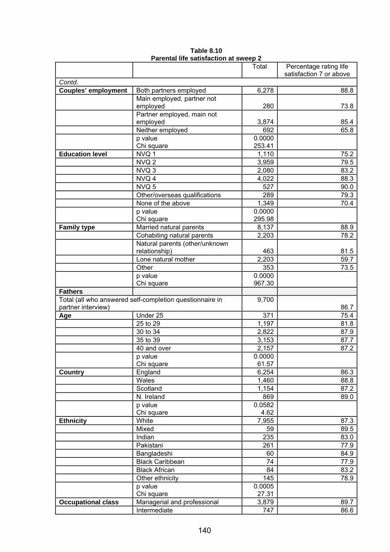
Table 8.10 Parental life satisfaction at sweep 2
Total Percentage rating life satisfaction 7 or above
Contd. Couples’ employment Both partners employed 6,278 88.8 Main employed, partner not
employed 280 73.8 Partner employed, main not
employed 3,874 85.4 Neither employed 692 65.8 p value
Chi square 0.0000253.41
Education level NVQ 1 1,110 75.2 NVQ 2 3,959 79.5 NVQ 3 2,080 83.2 NVQ 4 4,022 88.3 NVQ 5 527 90.0 Other/overseas qualifications 289 79.3 None of the above 1,349 70.4 p value
Chi square 0.0000295.98
Family type Married natural parents 8,137 88.9 Cohabiting natural parents 2,203 78.2 Natural parents (other/unknown
relationship) 463 81.5 Lone natural mother 2,203 59.7 Other 353 73.5 p value
Chi square 0.0000967.30
Fathers Total (all who answered self-completion questionnaire in partner interview)
9,70086.7
Age Under 25 371 75.4 25 to 29 1,197 81.8 30 to 34 2,822 87.9 35 to 39 3,153 87.7 40 and over 2,157 87.2 p value
Chi square 0.0000
61.57 Country England 6,254 86.3 Wales 1,460 88.8 Scotland 1,154 87.2 N. Ireland 869 89.0 p value
Chi square 0.0582
4.62 Ethnicity White 7,955 87.3 Mixed 59 89.5 Indian 235 83.0 Pakistani 261 77.9 Bangladeshi 60 84.9 Black Caribbean 74 77.9 Black African 84 83.2 Other ethnicity 145 78.9 p value
Chi square 0.0005
27.31 Occupational class Managerial and professional 3,879 89.7 Intermediate 747 86.6
140

Table 8.10 Parental life satisfaction at sweep 2
Total Percentage rating life satisfaction 7 or above
Contd. Small employer and self employed 1,398 88.6 Lower supervisory and technical 1,360 84.3 Routine and semi-routine 2,304 79.9 p value
Chi square 0.0000119.41
Couples’ employment Both partners employed 5,505 88.4 Main employed, partner not
employed 239 75.7 Partner employed, main not
employed 3,342 87.0 Neither employed 606 67.7 p value
Chi square 0.0000178.33
Education level NVQ 1 621 82.3
NVQ 2 2,547 86.2 NVQ 3 1,434 87.2 NVQ 4 2,946 88.4 NVQ 5 616 91.6 Other/overseas qualifications 327 80.9 None of the above 893 81.9 p value
Chi square 0.0000
54.56 Family type Married natural parents 7,258 88.9 Cohabiting natural parents 1,791 79.2 Natural parents (other/unknown
relationship) 471 79.8 Other 217 78.0 p value 0.0000
Chi square 142.39 Variable used for weighting: weight 2, apart from analysis by country which uses weight 1. Lone fathers not included. Height and weight All main and partner respondents (except pregnant women) were asked to give their weight at sweep 2. New respondents were also asked to give their height. At both sweeps height and weight could be reported in either metric (centimetres/kilograms) or imperial (feet and inches/stones and pounds) measures. Using these data, height in metres and weight in kilograms was derived for main and partner respondents. These variables were used to calculate Body Mass Index (BMI). This is the ratio of height and weight; weight in kilograms divided by height in metres, squared. BMI can be used to measure obesity. The following cut-offs were used: under 18.5 (underweight), 18.5 to 25 (normal weight), over 25 to 30 (overweight), over 30 to 35 (obese) and over 35 (morbidly obese). For both mothers and fathers there were variations in BMI by age, ethnic group, social class, couple work status and family type, but not country (Table 8.11). Mothers’ BMI BMI showed few clear patterns of variation with age, although the relationship was statistically significant. Younger mothers, however, were more likely to be
141

underweight than older mothers; 6.7 per cent among those under 25, compared with 2.1 per cent of those aged 40 and over. BMI showed significant variation by ethnic group; Black Caribbean and Black African mothers were much more likely than White ones to be overweight (32.2 per cent and 36.6 per cent compared with 25.1 per cent), obese (27.2 per cent and 17.0 per cent compared with 9.7 per cent) and morbidly obese (5.9 per cent and 8.7 per cent compared with 3.9 per cent). Pakistani mothers were also more likely than White mothers to be obese (15.5 per cent) but similar proportions were overweight and morbidly obese. Bangladeshi mothers were more likely than White ones to be overweight (41.3 per cent) and obese (13.0 per cent) but much less likely to be morbidly obese (0.9 per cent). Mothers in lower supervisory and technical or routine and semi-routine occupations were the most likely to be obese or morbidly obese; almost one in five of these groups had a BMI of 30 or above. The more educated mothers (NVQ level 4 and 5) were less likely to be obese or morbidly obese than the less educated (NVQ level 1 and 2) or those lacking qualifications. BMI also varied significantly by couples’ employment status and family type, though few notable patterns were observed. Fathers BMI showed few clear patterns of variation with age, although the relationship was statistically significant. BMI varied by ethnic group. Black African fathers were more likely than White fathers to be overweight (50.1 per cent compared with 46.1 per cent) and obese (19.3 per cent compared with 13.3 per cent) and morbidly obese (3.9 per cent compared with 3.5 per cent), though these differences were not as large as for mothers. Black Caribbean fathers were also more likely than White ones to be overweight (48.8 per cent) but less likely to be obese (8.5 per cent) or morbidly obese (1 per cent). Pakistani fathers were less likely than White fathers to be overweight (39.3 per cent) but similar proportions were obese and morbidly obese. Bangladeshi fathers were less likely than White fathers to be overweight (30.1 per cent), obese (8.1 per cent) and morbidly obese (1.6 per cent). Fathers in routine and semi-routine occupations were the most likely to be obese or morbidly obese; almost one in five had a BMI of 30 or over. Fathers in couples in which neither partner was employed were the most likely to be obese or morbidly obese (nearly one in five and 9.2 per cent morbidly obese). The more educated fathers (NVQ level 4 and 5) were less likely to be obese or morbidly obese than the less educated (NVQ level 1 and 2) or those lacking qualifications. BMI also varied significantly by family type, though few notable patterns were observed.
Table 8.11 Parental Body Mass Index at sweep 2
Total BMI Less than 18.5
(underweight) 18.5 to
25.0 (normal)
Over 25 to 30 (overweight)
Over 30 to 35
(obese)
Over 35 (morbidly obese)
% % % % % Mothers Total (all who completed main interview) 12,822 2.9 57.9 25.3 9.9 4.0Age Under 25 1,696 6.7 56.6 22.0 10.4 4.2 25 to 29 2,410 3.9 53.6 25.7 12.0 4.8 30 to 34 4,108 2.5 58.1 26.0 9.7 3.8 35 to 39 3,376 1.7 59.8 26.2 8.9 3.5 40 and over 1,226 2.1 59.9 23.9 9.5 4.6
142

Table 8.11 Parental Body Mass Index at sweep 2
Total BMI Less than 18.5
(underweight) (normal)
Over 25 to 30 (overweight)
Over 30 to 35
(obese)
Over 35 (morbidly obese)
18.5 to 25.0
% % % % % Contd. p value
Chi square 0.0000143.08
Country England 8,228 3.0 57.9 25.2 9.9 4.0 Wales 1,879 3.3 56.5 26.0 10.3 3.9 Scotland 1,482 2.4 60.7 24.0 9.0 3.9 N. Ireland 1,233 2.0 55.3 30.3 8.8 3.6 p value
Chi square 0.0690
27.75
Ethnicity White 10,682 2.7 58.6 25.1 9.7 3.9 Mixed 107 5.1 60.3 21.7 9.2 3.6 Indian 313 6.3 60.3 24.8 5.8 2.8 Pakistani 486 5.2 47.8 27.2 15.5 4.2 Bangladeshi 171 2.4 42.5 41.3 13.0 0.9 Black Caribbean 151 3.6 31.1 32.2 27.2 5.9 Black African 164 3.6 34.1 36.6 17.0 8.7 Other ethnicity 209 4.5 61.3 23.7 6.9 3.6 p value
Chi square 0.0000139.25
Occupational class
Managerial and professional 2,510 1.5 63.9 23.2 8.8 2.6
Intermediate 1,604 2.5 57.4 25.8 10.1 4.2 Small employer
and self-employed 455 3.0 60.3 25.3 8.8 2.6
Lower supervisory and technical 265 0.8 51.1 28.1 13.0 7.1
Routine and semi-routine 1,845 3.1 52.3 26.6 12.4 5.5
p value Chi square
0.000097.38
Couples’ employment
Both partners employed 5,801 1.9 58.8 25.1 10.3 3.8
Main employed, partner not employed 258 4.2 58.4 20.5 10.4 6.5
Partner employed, main not employed 3,829 2.5 58.0 26.6 9.2 3.7
Neither employed 729 6.5 51.8 24.5 10.1 7.1
p value Chi square
0.000075.57
Education NVQ 1 1,036 4.4 53.7 25.3 10.9 5.7 NVQ 2 3,699 3.3 54.2 26.7 11.1 4.6 NVQ 3 1,887 1.8 58.3 24.6 11.0 4.3 NVQ 4 3,729 1.9 63.2 24.1 7.9 2.9 NVQ 5 505 3.4 71.6 18.5 5.9 0.6 Other/overseas
qualifications 386 5.3 50.7 28.8 10.1 5.2
143

Table 8.11 Parental Body Mass Index at sweep 2
Total BMI Less than 18.5
(underweight) (normal)
Over 25 to 30 (overweight)
Over 30 to 35
(obese)
Over 35 (morbidly obese)
18.5 to 25.0
% % % % % Contd. None of the
above 1,574 5.2 48.4 28.8 12.3 5.3 p value
Chi square 0.0000242.41
Family type Married natural parents 7,908 2.0 58.5 25.7 9.9 3.9
Cohabiting natural parents 1,999 4.0 57.2 25.5 9.2 4.0
Natural parents (other/unknown relationship) 467 2.0 56.3 25.3 12.3 4.1
Lone natural mother 2,166 5.9 56.3 24.0 10.0 3.9
Other 282 3.6 58.5 21.4 9.9 6.6 p value
Chi square 0.0000
103.34 Fathers Total (all who completed partner interview) 8,726 0.5 37.2 45.7 13.2 3.5Age Under 25 290 1.2 51.5 32.9 10.0 4.3 25 to 29 1,046 1.3 44.3 38.3 12.5 3.7 30 to 34 2,525 0.6 37.0 45.0 14.6 2.7 35 to 39 2,873 0.4 35.3 47.8 12.6 3.8 40 and over 1,960 0.2 35.3 48.0 13.0 3.5 p value
Chi square 0.0000
83.62 Country England 5,674 0.5 37.3 45.4 13.2 3.5 Wales 1,256 0.4 34.1 48.5 14.2 2.8 Scotland 1,024 0.5 38.2 46.4 12.2 2.6 N. Ireland 772 1.2 33.1 47.6 13.7 4.5 p value
Chi square 0.0576
24.46 Ethnicity White 7,675 0.5 36.6 46.1 13.3 3.5 Mixed 59 50.1 37.7 10.0 2.2 Indian 254 1.2 43.0 42.0 10.3 3.6 Pakistani 308 2.8 40.7 39.3 13.2 3.9 Bangladeshi 87 60.2 30.1 8.1 1.6 Black Caribbean 71 41.6 48.8 8.5 1.0 Black African 89 26.7 50.1 19.3 4.0 Other ethnicity 165 1.7 43.4 38.2 12.8 3.9 p value
Chi square 0.0439
53.38 Occupational class
Managerial and professional 3,522 0.3 36.8 46.8 13.2 2.9
Intermediate 664 0.5 34.2 48.3 13.5 3.5 Small employer
and self-employed 1,249 0.3 38.1 47.2 11.1 3.3
Lower supervisory and technical 1,214 0.6 37.0 46.4 12.6 3.4
144

Table 8.11 Parental Body Mass Index at sweep 2
Total BMI Less than 18.5
(underweight) (normal)
Over 25 to 30 (overweight)
Over 30 to 35
(obese)
Over 35 (morbidly obese)
18.5 to 25.0
% % % % % Contd. Routine and
semi-routine 2,031 1.2 38.7 40.4 14.7 5.0 p value 0.0002
59.07 Chi square Couples’ employment
Both partners employed 4,941 0.2 36.2 47.2 12.9 3.5
Main employed, partner not employed 193 1.5 43.7 44.0 8.7 2.1
Partner employed, main not employed 2,992 0.5 37.8 44.9 13.9 2.8
Neither employed 561 3.8 42.3 32.5 12.2 9.2
p value 0.0000167.92 Chi square
Education NVQ 1 572 2.2 31.1 41.4 19.6 5.7 NVQ 2 2,322 0.6 35.1 46.9 14.0 3.5 NVQ 3 1,352 0.5 35.4 46.7 13.8 3.6 NVQ 4 2,750 0.1 38.6 46.4 12.2 2.7 NVQ 5 560 0.5 44.9 45.5 8.5 0.6 Other/overseas
qualifications 298 1.4 41.9 42.4 9.5 4.8 None of the
above 867 0.5 38.0 40.7 13.8 7.1 p value
Chi square 0.0000158.36
Family type Married natural parents 6,607 0.4 36.5 46.8 12.8 3.4
Cohabiting natural parents 1,473 0.8 39.5 42.0 14.5 3.2
Natural parents
(other/unknown relationship) 461 0.6 37.5 44.1 13.9 3.9
Other 185 2.6 44.3 34.5 13.7 4.8 p value
Chi square 0.0015
38.89 Note: Total bases are unweighted. Percentages are weighted. Variable used for weighting: weight 2, apart from analysis by country which uses weight 1. Lone fathers not included.
Conclusion Most parents seem to be in reasonably good health, as would be expected of adults with children of this age. Around 30 per cent smoked, and the large majority drank alcohol at some time, though problem drinking appeared rare. Mild mental health problems were fairly common for these parents, though not necessarily current during the survey. At that time, the vast majority (around five out of six) said they
145

were reasonably satisfied with their lives. There were, of course, exceptions, and differences in physical and mental health and related behaviours varied by gender, country, age and socio-economic circumstances. The socio-economic patterning of health forms part of the constellation of deprivation in which some of the cohort children are growing up.
References Bracken, B. A. (1998). Bracken. Basic Concept Scale - Revised. San Antonio, Texas: The Psychological Corporation.
Bracken, B. A. (2002). Bracken School Readiness Assessment Administration Manual. San Antonio, TX: The Psychological Corporation.
Bricker, D., Squires, J., Mounts, L., Potter, L., Nickel, B., & Farrell, J. (1995). Ages and Stages Questionnaire. Baltimore: Paul H. Brookes.
Elliott, C. D. (1983). British Ability Scales. Windsor, UK: NFER-Nelson.
Fenson, L., Dale, P. S., Resnick, J. S., Thal, D., Bates, E., Hartung, J. P., et al. (1993). MacArthur Communicative Development Inventories (CDI). San Diego, CA: Singular Publishing Group.
Frankenburg, W. K., & Dodds, J. B. (1967). Denver Developmental Screening Test J. Paediatrics, 71, 181-191.
Frankenburg, W. K., & Dodds, J. B. (1990). Denver II screening manual. Denver, CO: Denver Developmental Materials.
Goodman, R. (1997). The Strengths and Difficulties Questionnaire: A Research Note
Journal of Child Psychology and Psychiatry, 38, 581-586.
Goodman, R. (2001). Psychometric properties of the Strengths and Difficulties Questionnaire (SDQ) Journal of the American Academy of Child and Adolescent Psychiatry, 40(1337-1345).
Elliot, C.D., Smith, P. & McCulloch, K. (1997) British Abilities Scale II Technical Manual. London, UK: NFER-Nelson.
Goodman, R., Meltzer, H., & Bailey, V. (1998). The Strengths and Difficulties Questionnaire: A pilot study on the validity of the self-report version, European Child and Adolescent Psychiatry, 7, 125-130.
Moon, N. (2006) Technical Report on Fieldwork, London: NOP. http://www.cls.ioe.ac.uk/studies.asp?section=00010002000100040006
Schoon, I., Sacker, A., Hope, S., Collishaw, S., & Maughan, B. (2005). Children’s development in the family environment. In S. Dex & H. Joshi (Eds.), Babies of the New Millennium (pp. 159-174): Polity Press
146

Chapter 9 EMPLOYMENT AND EDUCATION Kelly Ward and Shirley Dex Introduction The economic activity and employment of parents is one vitally important element of the context in which the cohort child is growing up. It influences both the time available to spend with the child and the income level and household resources the child has grown up with. In this chapter, we report on the parents’ economic activity, employment and education. Chapter 10 focuses more particularly on the income consequences of these activities. It is well known that mothers’ employment has substantially increased since the 1960s and full-time working for mothers has increased markedly since 1985. This has been largely due to mothers with young children entering the labour market, the type of mothers, in fact, who are parents of the Millennium Cohort Study’s three-year-old children. Between the two sweeps, we expect to see some changes in mothers’ employment as well as continuity for other mothers. This is a relatively short period but a time when children are changing very fast, so it is interesting to see the extent of change in their parents’ employment status. We can also examine how many parents have gained new academic or vocational qualifications in this two-year period – a feature of the data relevant to policies on lifelong learning. Parents’ employment at sweep 2 Mothers’ economic activity More than half of all mothers were employed and 42 per cent were looking after the family and home at the time of the survey of three-year-olds. Nearly 4 per cent were also not working for various reasons, including unemployment and being in education (just over 1 per cent each). Mothers in Scotland were more likely to report that they were working (62.4 per cent) compared to mothers in England (53.2 per cent). See Table 9.1. Approximately 13 per cent of all mothers reported working full-time and 41.1 per cent worked part-time. Mothers in Northern Ireland were most likely to be employed full-time (22.1 per cent) and mothers in Scotland were most likely to report working part-time (47 per cent). Nearly 47 per cent of mothers in England were not employed when their child was aged three. Of all employed mothers, approximately three-quarters worked part-time. Mothers’ employment rate of 54.3 per cent at sweep 2 (of those interviewed then) compares with 48.7 per cent who were employed when the child was nine months old (on the base of the higher sweep 1 sample). Of the mothers present at both surveys, the employment rate was 50.8 per cent at sweep 1, increasing to 54.3 per cent at sweep 2. This increase is the net result of 24.5 per cent entering employment between surveys and 17.3 per cent leaving employment. Further details of transitions
147
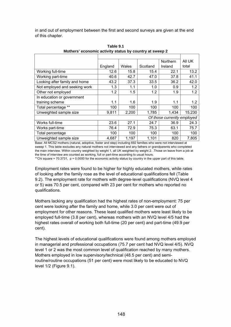
in and out of employment between the first and second surveys are given at the end of this chapter.
Table 9.1
Mothers’ economic activity status by country at sweep 2
England Wales Scotland Northern Ireland
All UK total
Working full-time 12.6 15.8 15.4 22.1 13.2Working part-time 40.6 42.7 47.0 37.8 41.1Looking after family and home 43.2 37.3 33.5 36.2 42.0Not employed and seeking work 1.3 1.1 1.0 0.9 1.2Other not employed 1.2 1.5 1.2 1.9 1.2In education or government training scheme 1.1 1.6 1.9 1.1 1.2Total percentage ** 100 100 100 100 100Unweighted sample size 9,811 2,200 1,785 1,434 15,230
Of those currently employed Works full-time 23.6 27.1 24.7 36.9 24.3Works part-time 76.4 72.9 75.3 63.1 75.7Total percentage 100 100 100 100 100Unweighted sample size 4,687 1,197 1,101 820 7,805
Base: All MCS2 mothers (natural, adoptive, foster and step) including 692 families who were not interviewed at sweep 1. This table excludes any natural mothers not interviewed and any fathers or grandparents who completed the main interview. Within country weighted by weight 1, all UK weighted by weight 2. .Those on leave from a job at the time of interview are counted as working, full or part-time according to usual hours. **Chi square = 70.3731, p = 0.0000 for the economic activity status by country in the upper part of this table. Employment rates were found to be higher for highly educated mothers, while rates of looking after the family rose as the level of educational qualifications fell (Table 9.2). The employment rate for mothers with degree-level qualifications (NVQ level 4 or 5) was 70.5 per cent, compared with 23 per cent for mothers who reported no qualifications. Mothers lacking any qualification had the highest rates of non-employment: 75 per cent were looking after the family and home, while 3.0 per cent were out of employment for other reasons. These least qualified mothers were least likely to be employed full-time (3.8 per cent), whereas mothers with an NVQ level 4/5 had the highest rates overall of working both full-time (20 per cent) and part-time (49.9 per cent). The highest levels of educational qualifications were found among mothers employed in managerial and professional occupations (75.7 per cent had NVQ level 4/5). NVQ level 1 or 2 was the most common level of qualification reached by many mothers. Mothers employed in low supervisory/technical (48.5 per cent) and semi-routine/routine occupations (51 per cent) were most likely to be educated to NVQ level 1/2 (Figure 9.1).
148

Table 9.2 Mothers’ current economic activity by highest educational achievement
Mothers’ highest education (academic or vocational) MCS2
NVQ level 4/5 Degree+
NVQ level 3 A-level
NVQ level 1/2 O-level GCSE
Overseas and other unclassified qualification
None of these
All UK total
Employed full-time 20.0 14.7 9.0 6.8 3.8 13.2Employed part-time 49.9 44.4 39.3 17.2 17.6 41.2Looking after family and home 27.5 35.9 47.8 71.3 75.0 41.9Other not employed or unemployed 1.6 2.8 3.0 3.2 3.0 2.5In education 1.1 2.2 1.0 1.5 0.7 1.2Total percentage ** 100 100 100 100 100 100Unweighted sample size 4,887 2,226 5,548 477 2,060 15,198Of those currently employed Works full-time 28.6 24.9 18.6 28.3 17.6 24.3Works part-time 71.4 75.1 81.4 71.7 82.4 75.7Total percentage 100 100 100 100 100 100Unweighted sample size 3,445 1,312 2,562 98 384 7,801
Base: All MCS2 mothers (natural, adoptive, foster and step) including 692 families who were not interviewed at sweep 1. This table excludes any natural mothers not interviewed and any fathers or grandparents who completed the main interview: 32 natural mothers did not provide their educational qualifications. Weighted by all-UK weight. ** Chi square = 1512.46, p = 0.0000 for economic activity by NVQ in upper table only. Degree+ means this level is degree-level or above .
Figure 9.1 Employed mothers’ NS-SEC classification at sweep 2 by highest education level
0.8 2.5 3.39.9
13.64.9
13.0
38.6 35.4
48.5
51.0
31.610.5
24.3
19.6
16.5
17.8
16.5
75.7
34.641.8
25.017.5
47.0
0%
10%
20%
30%
40%
50%
60%
70%
80%
90%
100%
Managerial &professional
Intermediate Small employer &self-employed
Low supervisory &technical
Semi-routine &routine
All UK Total
NS-SEC
Perc
enta
ge (%
)
NVQ level 4/5NVQ level 3NVQ level 1/2None of these
Base: All employed MCS2 mothers (natural, adoptive, foster and step) including 692 families not interviewed at sweep 1. Mothers with overseas only qualifications and unclassified qualifications are included in ‘none’. Excludes mothers with no information on NS-SEC. Weighted by all-UK weight: Chi square = 2204.76, p value = 0.00 Mothers’ economic status varied significantly by the type of electoral ward in which they were sampled for sweep 1. Mothers sampled in non-disadvantaged wards were far more likely to be employed (59.4 per cent) than those in wards with high minority
149

ethnic populations (25.5 per cent). Seventy per cent of mothers originally living in wards with high minority ethnic populations reported that they were looking after the family and home compared to 46.8 per cent of mothers from other disadvantaged wards and 37.4 per cent of mothers from non-disadvantaged wards (Table 9.3).
Table 9.3 Mothers’ economic activity status at sweep 2 by electoral ward
Type of ward at MCS1
Minority ethnic (disadvantaged)
Other Disadvantaged
Non-disadvantaged
All UK Total
Currently working full-time 8.9 12.4 14.0 13.2Currently working part-time 16.6 36.3 45.4 41.1Looking after family and home 70.1 46.8 37.4 42.0Other not employed or unemployed* 2.6 3.0 2.2 2.5In education 1.8 1.6 0.9 1.2Total percentage ** 100 100 100 100Unweighted sample size 1,869 7,036 6,325 15,230Of those currently employed Works full-time 34.8 25.4 23.5 24.3Works part-time 65.2 74.6 76.5 75.7Total percentage 100 100 100 100Unweighted sample size 477 3,472 3,856 7,805
Base: All MCS2 mothers (natural, adoptive, foster and step) including 692 families who were not interviewed at sweep 1. This table excludes any natural mothers not interviewed and any fathers or grandparents who completed the main interview. Weighted by all-UK weight. ** Chi square = 403.67, p=0.00 for economic activity by area of residence in upper table only.
Turning to the individual’s ethnicity rather than the composition of the neighbourhood, we can see which ethnic groups were involved in the low employment rates in minority ethnic neighbourhoods and beyond. Pakistani and Bangladeshi mothers were least likely to be employed (13.9 per cent and 13.5 per cent respectively), whereas Indian (62.8 per cent), Black Caribbean (59.9 per cent) and White mothers (57.3 per cent) were most likely to be employed (Table 9.4). Around four out of five Pakistani and Bangladeshi mothers were looking after the family and home (Table 9.4). Black Caribbean (34.1 per cent), Black African (26.2 per cent) and Indian mothers (25.2 per cent) reported the highest rates of full-time employment. Mothers of White (44.2 per cent) and Indian (37.6 per cent) ethnicity were most likely to be working part-time.
Table 9.4
Mothers’ economic activity status at sweep 2 by ethnicity
White Indian Pakistani Bangladeshi Black Caribbean
Black African Other
All UK total
Working full-time 13.1 25.2 3.1 2.3 34.1 26.2 17.4 13.5Working part-time 44.2 37.6 10.8 11.2 25.9 22.6 19.9 42.0Looking after family and home 39.2 36.0 83.3 83.9 32.0 43.8 55.7 41.0Other not employed or unemployed 2.4 0.8 1.9 2.6 5.4 1.8 3.6 2.4In education 1.0 0.4 0.9 0.0 2.6 5.7 3.5 1.1Total percentage ** 100 100 100 100 100 100 100 100Sample size 1,2474 366 652 247 178 240 385 14,542
150

Table 9.4 Mothers’ economic activity status at sweep 2 by ethnicity
White All UK total Indian Pakistani Bangladeshi Black
CaribbeanBlack African Other
Contd. Of those currently employed Works full-time 22.9 40.1 22.3 17.1 56.9 53.6 46.6 24.3Works part-time 77.1 59.9 77.7 82.9 43.1 46.4 53.4 75.8Total percentage 100 100 100 100 100 100 100 100Unweighted sample size 6,981 201 70 28 99 87 127 7,593
Base: All MCS2 mothers (natural, adoptive, foster and step) including 692 families not interviewed at sweep 1. Excludes approximately 688 cases where mother’s ethnicity was not known. Weighted by all-UK weight. ** Chi square = 497.19, p = 0.0000 for economic activity by ethnicity in upper table only. Mother’s employment status was found to vary significantly by the number of children in the household (Table 9.5). Mothers who only had one child (the cohort member) were, not surprisingly, far more likely to be currently in paid work (66.6 per cent) compared to mothers with three or more children (39.7 per cent). The reverse was also true for mothers who reported they were currently looking after the family and home: 57.2 per cent of mothers with three or more children were looking after the family compared to only 27.9 per cent of mothers with one child. Part-time was far more common than full-time working for all mothers who were employed, regardless of the number of children. Employed mothers who had one child were more likely to work full-time (31.3 per cent) compared to mothers who had two children (22.1 per cent) or mothers with three or more children (19.7 per cent).
Table 9.5
Mothers’ economic activity status by number of children at sweep 2 Number of children living in household
Cohort baby only
Two children
Three or more children
All UK total
Working full-time 20.8 12.5 7.8 13.2Working part-time 45.8 44.2 31.8 41.1Looking after family and home 27.9 40.3 57.2 42.0Other not employed or unemployed 3.5 2.2 2.1 2.5In education or government training scheme 1.9 0.9 1.1 1.2Total percentage ** 100 100 100 100Unweighted sample size 3,729 6,850 4,651 15,230Of those currently employed Works full-time 31.3 22.1 19.7 24.3Works part-time 68.7 77.9 80.3 75.7Total percentage 100 100 100 100Unweighted sample size 2,385 3,740 1,680 7,805
Base: All MCS2 mothers (natural, adoptive, foster and step) including 692 families who were not interviewed at sweep 1. Weighted by all-UK weight. ** Chi square = 733.03, p = 0.0000 for economic activity by number of children in upper table only.
151

Resident fathers’ economic activity at sweep 2 The Millennium Cohort Study did not collect information about the economic activity of non-resident fathers. Hence the discussion about fathers’ employment in this section refers only to resident fathers. Nearly all resident fathers (92.4 per cent) were employed when the child was aged three, mostly (74 per cent) as employees. Some 18.4 per cent of fathers were self-employed (Table 9.6). The rate of self-employment among fathers is an increase over the MCS1 rate of 15.7 per cent. Fathers in Northern Ireland (24.1 per cent) and England (18.8 per cent) had higher rates of self-employment than fathers in Wales (15.3 per cent) or Scotland (14.3 per cent). These rates of self-employment for fathers of Millennium children are higher than the average rate of self-employment across the male working population, which in 2003 was 16 per cent across the UK (Labour Force Survey in Labour Market Trends). Approximately 7.6 per cent of fathers were not employed when the cohort child was aged three. This compares with 9 per cent of all UK fathers with a youngest child aged 0-4 in 2004. Five per cent of employed MCS fathers worked part-time.
Table 9.6
Resident fathers’ economic activity by country at sweep 2
England Wales Scotland Northern Ireland All UK total
Employee 73.7 76.0 77.4 68.7 74.0Self-employed 18.8 15.3 14.3 24.1 18.4Not employed 7.5 8.7 8.2 7.2 7.6Total percentage ** 100 100 100 100 100Unweighted sample size 6707 1488 1169 892 10256Of those currently employed Works full-time 94.4 94.4 94.9 94.9 94.5Works part-time 5.6 5.6 5.1 5.1 5.5Total percentage 100 100 100 100 100Unweighted sample size 6,032 1,333 1,059 811 9,235
Base: All MCS2 fathers (natural, adoptive, foster and step) including 692 families who were not interviewed at sweep 1. Excludes fathers who were present at MCS2 but not interviewed or provided proxy information, and other carers who completed the partner interview (mothers and grandparents). Within country weighted by weight 1, all-UK weighted by weight 2. ** Chi square= 20.09, p = 0.001 for father’s economic activity by country in upper table only. As with mothers, employment rates for fathers were higher for more highly qualified individuals, yet interestingly rates of self-employment increased slightly as the level of educational qualifications fell (Table 9.7). Of fathers with an NVQ level 4 or 5 qualification, 81.4 per cent were employees, compared to 52.9 per cent of those who reported no qualifications. Approximately a quarter of fathers who had no academic or vocational qualifications were not employed. This compared with an average of 7 per cent who were not employed across all levels of qualification. Employed fathers with an overseas qualification (13.1 per cent) or no qualification (14.2 per cent) were more likely to be working part-time compared to fathers with some qualifications, of whom 4 to 5 per cent worked part-time.
152
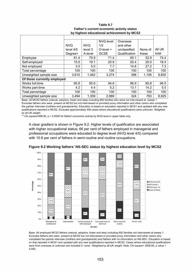
Table 9.7 Father’s current economic activity status
by highest educational achievement by MCS2
NVQ level 4/5 Degree+
NVQ level 3
NVQ level 1/2 O-level + GCSE
Overseas and other unclassified Qualification
None of these
All UK total A-level
Employee 81.4 75.9 71.4 65.1 52.9 74.4Self-employed 15.5 19.1 20.9 20.4 20.0 18.4Not employed 3.0 5.0 7.7 14.6 27.2 7.3Total percentage 100 100 100 100 100 100Unweighted sample size 3,610 1,462 3,274 398 1,106 9,850Of those currently employed Works full-time 95.8 95.6 94.8 86.9 85.8 94.5Works part-time 4.2 4.4 5.2 13.1 14.2 5.5Total percentage 100 100 100 100 100 100Unweighted sample size 3,494 1,359 2,969 324 783 8,929Base: All MCS2 fathers (natural, adoptive, foster and step) including 692 families who were not interviewed at sweep 1 Excludes fathers who were present at MCS2 but not interviewed or provided proxy information and other carers who completed the partner interview (mothers and grandparents). Education is based on education reported in MCS1 and updated with any new qualifications reported in MCS2. Excludes approximately 406 cases where educational qualifications were unknown. Weighted by all-UK weight. ** Chi square=698.90, p = 0.0000 for father’s economic activity by NVQ level in upper table only.
A clear gradient is shown in Figure 9.2. Higher levels of qualification are associated with higher occupational status; 66 per cent of fathers employed in managerial and professional occupations were educated to degree level (NVQ level 4/5) compared with 10.6 per cent of fathers in semi-routine and routine occupations. Figure 9.2 Working fathers’ NS-SEC status by highest education level by MCS2
3.4 4.9
16.7 13.1
26.9
11.4
18.0
27.8
44.846.3
49.9
32.712.6
19.7
17.7 21.2
12.6
15.0
66.0
47.7
20.7 19.410.6
40.9
0%
10%
20%
30%
40%
50%
60%
70%
80%
90%
100%
Managerial &professional
Intermediate Small employer &self-employed
Low supervisory &technical
Semi-routine &routine
All UK Total
NS-SEC
Perc
enta
ge NVQ level 4/5NVQ level 3NVQ level 1/2None of these
Base: All employed MCS2 fathers (natural, adoptive, foster and step) including 692 families not interviewed at sweep 1. Excludes fathers who were present at MCS2 but not interviewed or provided proxy information and other carers who completed the partner interview (mothers and grandparents) and fathers with no information on NS-SEC. Education is based on that reported in MCS1 and updated with any new qualifications reported in MCS2. Cases where educational qualifications were from overseas or unknown are included in ‘none’. Weighted by all-UK weight. Note: Chi square= 2836.65, p value = 0.000.
153

Pakistani (26.6 per cent), Indian (22.6 per cent) and Bangladeshi fathers (21.6 per cent) were the most likely to be self-employed, whereas White (75.8 per cent) and Black Caribbean fathers (71.1 per cent) were the most likely to be employees (Table 9.8). Working full-time was highest among fathers of White (95.4 per cent), Indian (93.1 per cent), Black African (92.2 per cent) and Black Caribbean (91 per cent) ethnicity compared to Bangladeshi (57.2 per cent) and Pakistani (78.4 per cent) fathers. Interestingly, nearly 43 per cent of employed Bangladeshi fathers were in part-time employment compared to around 4 per cent of employed White fathers.
Table 9.8 Fathers’ economic activity status at sweep 2 by ethnicity
White Indian Pakistani Bangladeshi Black Caribbean
Black African Other
All UK Total
Employee 75.8 70.1 54.3 59.7 71.1 68.8 70.2 74.9Self-employed 17.7 22.6 26.6 21.6 16.2 15.6 17.8 18.0Not employed 6.5 7.3 19.1 18.7 12.8 15.7 12.0 7.1Total percentage ** 100 100 100 100 100 100 100 100Unweighted sample size 8114 268 350 107 82 103 246 9,270Of those currently working Works full-time 95.4 93.1 78.4 57.2 91.0 92.2 88.3 94.6Works part-time 4.6 6.9 21.6 42.8 9.0 7.8 11.7 5.4Total percentage 100 100 100 100 100 100 100 100Unweighted sample size 7,460 243 283 86 69 78 206 8,425
Notes: All MCS2 fathers (natural, adoptive, foster and step) including 692 families who were not interviewed at sweep 1 Excludes fathers who were present at MCS2 but not interviewed or provided proxy information and other carers who completed the partner interview (mothers and grandparents). Excludes approximately 986 cases where father’s ethnicity was not known. Weighted by all-UK weight. Note: small sample sizes for Black Caribbean and Black African fathers. ** Chi square = 98.59, p = 0.0000 for father’s economic activity by ethnicity in upper table only. Parents’ employment status at sweep 2 By the time the cohort child was aged three, one in six was living in a family with no earner (15.8 per cent). This was mostly the 11.2 per cent whose lone parent was not employed. The most common situation was two parents in a 1.5-earner partnership, with the father employed full-time and the mother employed part-time (34.1 per cent). A further quarter of families (28.6 per cent) were couples where the father was the sole earner (Table 9.9). This arrangement was most common among mothers in England (29.6 per cent) compared to mothers in the other three countries (approximately 23 per cent). White (36.8 per cent) and Indian mothers (32.6 per cent) were most likely to live in families where the father was employed full-time and the mother part-time. Most Pakistani (58.9 per cent) and Bangladeshi mothers (50.4 per cent) were living in families where the father alone was employed. This arrangement was far less common among Black African (14.7 per cent) and Black Caribbean (10.6 per cent) mothers. Indian mothers reported the highest frequency of living in the type of two-parent family where both parents were employed full-time (25.9 per cent). Pakistani (2 per cent) and Bangladeshi (2.5 per cent) mothers were the least likely to live in a two-full-time-earner family (Table 9.10).
154

Table 9.9 Parents’ partnerships and economic status by country at sweep 2
England Wales Scotland Northern Ireland
All UK total
Both employed full-time 10.1 12.6 13.7 19.7 10.8Father full-time, mother part-time 33.8 35.5 36.7 30.2 34.1Father part-time, mother full-time 2.2 2.5 2.5 2.3 2.2Mother employed, father not employed 2.0 1.7 2.8 2.3 2.1Father employed, mother not employed 29.6 23.1 23.6 23.0 28.6Both not employed 4.6 5.7 4.2 3.7 4.6Lone parent employed 6.4 6.3 7.6 7.9 6.4Lone parent not employed 11.3 12.7 8.8 11.0 11.2Total percentage 100 100 100 100 100Unweighted sample size 8,646 1,949 1,432 1,152 13,179
All MCS2 mothers and fathers (natural, adoptive, foster and step) including 692 families who were not interviewed at sweep 1. Excludes mothers whose partners did not complete the interview (approximately 2,056 cases) and interviews completed by grandparents or proxy interviews. Weighted by all-UK weight. Chi square = 90.07, p = 0.0000.
Table 9.10 Parents’ partnerships and economic status by mother’s ethnicity
Mother’s ethnicity
White Indian Pakistani Bangladeshi Black Caribbean
Black African Other
All UK Total
Both employed full-time 10.9 25.9 2.0 2.5 19.6 17.7 11.2 11.1Father full-time and mother part-time 36.8 32.6 7.1 7.2 14.6 14.5 17.1 35.0Father part-time and mother full-time 2.2 4.1 2.6 3.1 2.4 5.1 2.4 2.2Mother employed, father not employed 1.9 2.6 4.4 5.8 2.5 0.8 2.1 2.0Father employed, mother not employed 28.0 23.6 58.9 50.4 10.6 14.7 36.8 28.6Both not employed 4.0 4.9 13.0 17.8 2.4 9.2 7.7 4.4Lone parent employed 6.3 2.8 2.3 3.1 20.6 9.1 5.8 6.3Lone parent not employed 10.0 3.5 9.8 10.3 27.3 29.0 16.9 10.4Total percentage 100 100 100 100 100 100 100 100Unweighted sample size 10,889 315 482 154 168 200 349 12,557
Base: All MCS2 mothers and fathers (natural, adoptive, foster and step) including 692 families who were not interviewed at sweep 1. Excludes mothers whose partners did not complete the interview (approximately 2,056 cases) and interviews completed by grandparents or proxy interviews. Excludes cases were ethnicity was unknown. Weighted by all-UK weight. Chi square = 647.52, p = 0.0000
Employed parents’ NS-SEC statuses Nearly 40 per cent of all employed mothers in the UK were in managerial/professional occupations, either high or low, when the child was aged three (Table 9.11). There were relatively minor variations across countries. Employed mothers in England had slightly higher rates in small employer and self-employed occupations (8.5 per cent) compared to mothers in Northern Ireland (5.2 per cent).
155

Table 9.11
Employed mothers’ MCS2 NS-SEC status by country Country at MCS2 England Wales Scotland N Ireland
All UK total
High managerial/professional 7.8 7.0 7.9 7.0 7.7Low managerial/professional 31.5 34.7 34.2 31.5 31.9Intermediate 24.4 21.7 23.3 27.8 24.2Small employer and self-employed 8.5 5.6 5.8 5.2 7.9Low supervisory 3.9 5.1 3.6 2.8 3.9Semi-routine 17.4 18.2 18.0 19.8 17.6Routine 6.6 7.7 7.2 5.9 6.7Total percentage 100 100 100 100 100Unweighted sample size 4,591 1,178 1,074 804 7,647
Base: All MCS2 employed mothers (natural, adoptive, foster and step) including 692 families who were not interviewed at sweep 1 whose occupations were known. Within country weighted by weight 1. All-UK weighted by weight 2. Chi square = 22.94, p = 0.08. Forty-four per cent of all employed fathers in the UK were in managerial occupations (high or low) when the cohort child was aged three (Table 9.12). This is a very slight increase on the sweep 1 data about employed fathers. These occupation groups were lowest for employed fathers living in Northern Ireland (33 per cent). But this was compensated for by higher proportions than other UK countries being in intermediate (10.2 per cent), small employer/self-employed (20.9 per cent) or routine occupations (15 per cent).
Table 9.12 Employed fathers’ NS-SEC status at sweep 2 by country
England Wales Scotland Northern Ireland
All UK total
High managerial/professional 15.7 11.2 14.5 11.0 15.2Low managerial/professional 29.7 29.0 26.7 22.1 29.1Intermediate 7.5 7.3 9.1 10.2 7.8Small employer and self-employed 14.7 12.4 11.2 20.9 14.6Low supervisory 12.5 16.4 15.9 12.3 12.9Semi-routine 9.3 9.0 9.1 8.3 9.3Routine 10.6 14.8 13.4 15.0 11.2Total percentage 100 100 100 100 100Unweighted sample size 6,656 1,476 1,164 885 10,181
Base: All MCS2 employed fathers (natural, adoptive, foster and step) including 692 families who were not interviewed at sweep 1. Excludes fathers who were present at MCS2 but not interviewed or provided proxy information and other carers who completed the partner interview (mothers and grandparents) and fathers with no information on NS-SEC. Within country weighted by weight 1. All-UK weighted by weight 2. Chi square = 64.13, p = 0.0000 Employed mothers’ atypical working patterns Mothers’ reports of atypical working hours, such as evenings, nights or weekends, varied only by country. Northern Ireland had lower amounts of such working than the other UK countries, particularly evenings and Saturdays or Sundays. Of all UK employed mothers, 35.1 per cent worked after 6 pm, 10.8 per cent reported working nights, 14 per cent worked on Saturday and 8.4 per cent on Sunday (Table 9.13). Overall, mothers in Northern Ireland were least likely to report working these atypical hours compared to mothers elsewhere.
156

Table 9.13 Percentage of employed mothers working atypical hours by country
Country at MCS2
England Wales Scotland Northern Ireland
All UK Total
Works after 6 pm* 35.4 33.4 35.4 30.4 35.1Works nights** 10.8 10.8 11.5 9.8 10.8Works Saturdays*** 13.7 15.2 16.2 10.5 14.0Works Sundays**** 8.4 9.8 8.8 4.1 8.4Works at any atypical time (any of the above) 42.9 41.6 42.7 35.8 42.6Unweighted sample size 4,779 1,205 1,107 826 7,917
Base: All employed MCS2 mothers (natural, adoptive, foster and step) including 692 families who were not interviewed at sweep 1, who reported working these atypical patterns on a weekly basis. Columns do not add up to 100 per cent as multiple responses allowed. *Chi-sq = 4.91, p = 0.25. ** Chi square = 4.03, P=0.28 *** Chi square=16.86, p = 0.01. **** Chi square=19.09, p = 0.01. A U-shaped social profile was found for mothers’ extent of working at atypical weekday hours by their current socio-economic status. Those in intermediate occupations were the least likely (22.3 per cent) to work after 6 pm. There was a more one-directional social gradient in weekend working. Mothers who reported working on Saturdays were most likely to be in small employer/self-employed; low supervisory/technical or semi-routine/routine occupations (Table 9.14).
Table 9.14 Employed mothers’ atypical weekly working patterns by NS-SEC status at sweep 2
Mothers working weekly atypical hours
Managerial and professional Intermediate
Small employer and self-employed
Low supervisory and technical
Semi-routine and routine
All UK Total
Works after 6 pm 35.2 22.3 42.5 46.5 43.9 35.2Works nights 10.5 5.5 9.0 19.3 16.0 10.9Works Saturdays 7.8 7.7 24.7 24.7 25.0 14.0Works Sundays 5.4 4.7 9.1 14.2 15.6 8.4Unweighted sample size 2,904 1,859 541 315 2,139 7,758
Base: All employed MCS2 mothers (natural, adoptive, foster and step) including 692 families who were not interviewed at sweep 1, who reported working these atypical patterns on a weekly basis. Columns do not add up to 100 per cent as multiple responses allowed. *Chi-sq = 499.62, p = 0.000. ** Chi square = 291.33, P=0.000 *** Chi square=657.33, p = 0.000. **** Chi square=481.00, p = 0.000.
Employee mothers’ flexible working arrangements Parents who were employees were asked at MCS2, ‘which, if any, of these arrangements have you made use of in your current main job, or, plan to make use of?’. The arrangements most commonly used by employee mothers were part-time working (63.7 per cent), flexible hours (29.5 per cent), changing from full to part-time working (23.4 per cent) and special shifts (16.8 per cent). Employee mothers in semi-routine/routine (71.3 per cent) and intermediate occupations (66.4 per cent) reported higher use of part-time working (Table 9.15). Use of special shifts was also highest among mothers in semi-routine/ routine (22.1 per cent) and low supervisory (24.2 per cent) occupations, compared to mothers in managerial and professional occupations (13.7 per cent). Employee mothers in managerial and professional occupations had
157

the highest rates of working at or from home occasionally (23.4 per cent). Clearly flexible working suits some jobs better than others. Flexible working, particularly part-time, varied significantly by country (Table 9.16). Compared with 63.7 per cent of all UK employee mothers working part-time, mothers in Northern Ireland reported the lowest frequencies (44.3 per cent) of part-time work. Nearly 65 per cent of White mothers reported part-time working compared to only 33 per cent of employed Black Caribbean and Black African mothers (Table 9.17). There was little variation by country in flexible working hours.
Table 9.15 Percentage of employee mothers in each NS-SEC group who reported using flexible
working at sweep 2 Mother’s NS-SEC at MCS2
Managerial and professional Intermediate
Low supervisory and technical
Semi-routine and routine
All UK total
P value
57.7 66.4 57.1 71.3 63.7 0.00Part-time working Job-sharing 11.6 10.3 6.3 3.6 8.8 0.00
32.2 33.6 26.7 21.8 29.5 0.00Flexible working hours Working at or from home occasionally 23.4 10.3 4.5 1.5 13.1
0.00
Working at or from home all the time 3.2 4.2 1.0 0.9 2.7
0.00
Special shifts (evenings, school hours) 13.7 14.8 24.2 22.1 16.8
0.00
Nine-day fortnights / 4.5-day working week 2.1 1.1 0.7 0.3 1.3
0.00
8.1 6.9 6.1 8.2 7.8 0.36School term-time contracts Ability to change from full-time to part-time 29.5 26.3 22.3 11.6 23.4
0.00
11.3 10.1 14.9 9.9 10.7 0.00None of these Unweighted maximum sample size 2,734 1,858 315 2,139 7,046
Base: All employee MCS2 mothers (natural, adoptive, foster and step) including 692 families not interviewed at sweep 1. Columns do not add up to 100 per cent as multiple responses allowed. Note: This table is based on employees only, therefore does not include self-employed mothers. Employees were asked ‘which, if any, of these arrangements have you made use of in your current main job, or, plan to make use of?’.
Table 9.16 Percentage of employee mothers in each country who reported flexible working arrangements at
sweep 2 Country
England Wales Scotland Northern Ireland
All UK total
P value
64.6 64.3 60.0 44.3 63.4 0.00Part-time working Job-sharing 8.6 7.8 11.2 6.7 8.7 0.02
30.0 30.4 27.4 27.7 29.7 0.29Flexible working hours 14.0 10.9 11.2 7.8 13.3 0.00Working at or from home occasionally 3.0 2.3 1.5 1.7 2.8 0.08Working at or from home all the time
16.9 17.4 15.3 10.6 16.6 0.00Special shifts (evenings, school hours) 1.3 1.3 1.1 2.3 1.3 0.28Nine-day fortnights / 4.5-day week
School term-time contracts 7.8 9.8 5.7 7.6 7.7 0.01
158

Table 9.16 Percentage of employee mothers in each country who reported flexible working arrangements at
sweep 2 Country
All UK total
P value
England Wales Scotland Northern Ireland
Contd. 24.0 22.4 20.5 22.6 23.5 0.41Ability to change from full- to part-time 10.4 11.9 11.4 19.2 10.8 0.00None of these
Unweighted cases sample size 4,279 1,109 1,025 775 7,188Base: All employee MCS2 mothers (natural, adoptive, foster and step) including 692 families not interviewed at sweep 1.
Table 9.17 Percentage of employee mothers in each ethnic group who reported using flexible
working arrangements with their current employer at sweep 2
White Indian Pakistani Black Caribbean
Black African Other All UK Total
Part-time working 64.9 53.9 54.2 33.2 33.1 46.2 63.6Job-sharing 9.1 2.1 11.6 3.5 4.7 1.9 8.7
Flexible working hours 29.3 33.5 37.5 36.0 31.8 33.1 29.7
Working at or from home occasionally 13.4 15.3 5.5 15.1 11.3 11.9 13.4
Working at or from home all the time 2.7 5.0 2.7 4.1 0.0 1.3 2.8
Special shifts (evenings, school hours) 16.8 14.2 12.3 12.6 7.8 21.9 16.7
Nine-day fortnights/ 4.5-day working week 1.4 1.2 0.0 4.3 0.0 0.9 1.4
School term-time contracts 7.6 9.1 13.0 6.8 6.1 4.1 7.7
Ability to change from full- to part-time 23.9 22.9 20.5 17.9 20.5 18.3 23.7
None of these 10.1 16.6 8.6 21.5 22.4 23.3 10.7
Unweighted cases sample size 6,396 196 72 96 82 118 6,992Base: All employee MCS2 mothers (natural, adoptive, foster and step) including 692 families who were not interviewed at sweep 1. Employee mothers were also asked ‘which, if any, of these arrangements have you made use of in your current main job, or, plan to make use of if currently away from work?’. The provisions most widely used by cohort mothers from their employers were time off for a family emergency (53.7 per cent) and use of a telephone in the workplace for family reasons (45.1 per cent). See Table 9.18. One in four employee mothers across the UK did not use any of the provisions listed. Employee mothers in Northern Ireland reported the highest frequency of needing time off for family emergencies (60 per cent) compared to mothers living in England (53.2 per cent) and Scotland (53.2 per cent). A relatively low proportion of mothers reported that they had benefited from financial help with childcare (8.7 per cent overall in the UK) and access to a workplace nursery or crèche (4.9 per cent). Each of these was used most by mothers living in England (9.5 per cent for financial help and 5.3 per cent for the workplace nursery) and used least by mothers in Northern Ireland (4.3 per cent for financial help and 1.5 per cent for the workplace nursery).
159

Non-employed mothers’ reasons for not working at sweep 2 Mothers neither working nor seeking work (nor on leave) when the cohort child was aged three were asked why they were not doing so (Table 9.19). In the UK as a whole, 63.7 per cent of these mothers reported that they preferred to be at home looking after their family. This figure varied significantly by country; ranging from 70.2 per cent of economically inactive mothers in Northern Ireland, to 56.4 per cent in Scotland.
Table 9.18
Percentage of employee mothers who used or planned to use employer-provided family-friendly arrangements by country at sweep 2
England Wales Scotland Northern Ireland
All UK total
p value
Financial help with childcare/childcare vouchers 9.5 5.5 5.7 4.3 8.7 0.00Workplace nursery or crèche 5.3 5.2 2.9 1.5 4.9 0.00Other nurseries supported by employer 1.0 1.1 0.6 0.8 0.9 0.65Help with finding childcare facilities away from the workplace 2.8 1.7 3.0 1.4 2.7 0.06Care for children after school hours or during school holidays 6.0 6.0 6.1 4.5 5.9 0.45Time off for family emergencies 53.2 57.8 53.2 60.0 53.7 0.00Career breaks for personal reasons* 7.0 8.5 9.8 6.9 7.4 0.13Parental leave* 15.9 15.8 18.7 17.2 16.2 0.43A telephone to use for family reasons 44.3 50.0 46.3 50.3 45.1 0.00None of these 24.4 20.5 24.5 19.7 24.1 0.00
Base: All MCS2 employee mothers (natural, adoptive, foster and step) including 692 families who were not interviewed at sweep 1. Columns do not add up to 100 per cent as multiple responses allowed. Note: This table is based on employees only therefore does not include self-employed mothers. Employees were asked ’which, if any, of these arrangements have you made use of in your current main job, or plan to make use of if currently away from work?’
Unweighted cases sample size 4,202 1,104 1,021 770 7,097
* The survey did not ask whether these benefits were paid or not. Of the economically inactive, 57.9 per cent reported that they preferred to look after their children themselves and 10.7 per cent reported that they were not working because they were unable to earn enough to pay for childcare. Citing these costs as a problem varied by country, from 11.4 per cent of responses in England to 7.9 per cent in Scotland, but the variations were not statistically significant (at 95 per cent level of confidence). Approximately 9 per cent of these mothers were at home because they had a new baby. There were small variations in the reasons mothers in couples gave for not being employed when the child was aged three, according to their partner’s employment status at the time (Table 9.20). Mothers who preferred to look after the child themselves were a slightly lower percentage of those with a non-employed partner (55.1 per cent) compared with mothers who had an employed partner (around 62 per cent). Mentioning problems of finding suitable childcare was most frequent (11 per cent) among mothers with full-time employed partners, and very infrequent (4.7 per
160
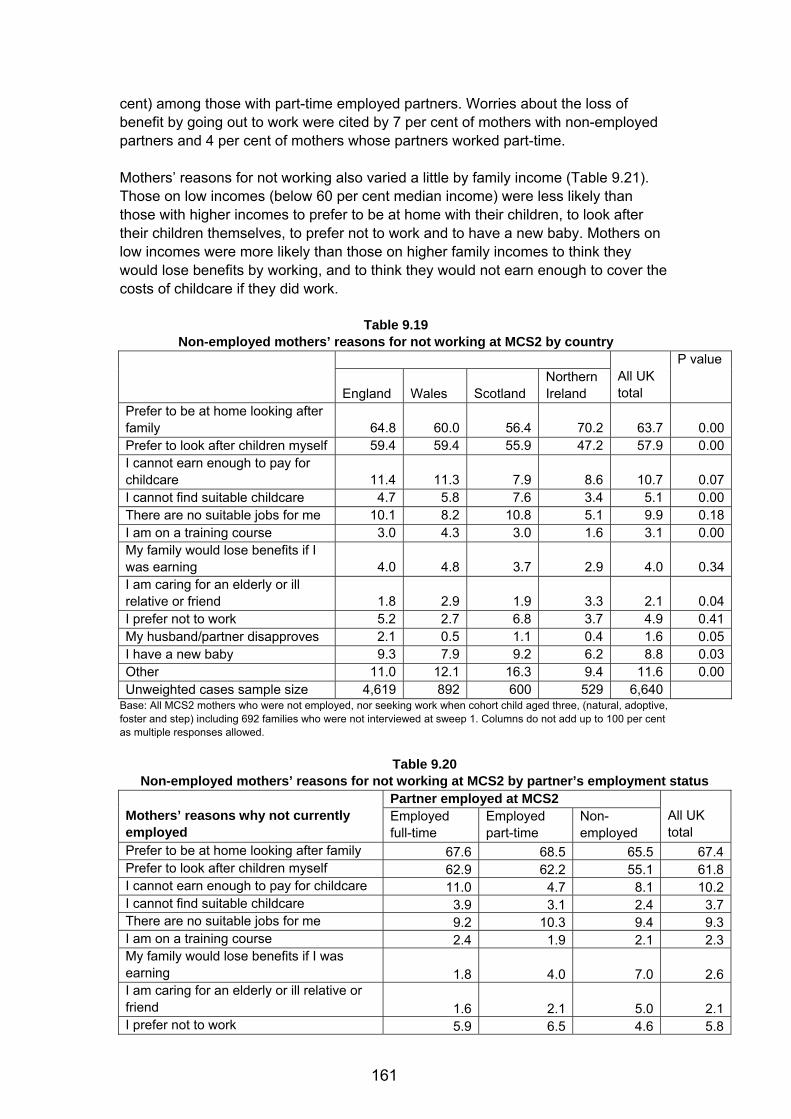
cent) among those with part-time employed partners. Worries about the loss of benefit by going out to work were cited by 7 per cent of mothers with non-employed partners and 4 per cent of mothers whose partners worked part-time. Mothers’ reasons for not working also varied a little by family income (Table 9.21). Those on low incomes (below 60 per cent median income) were less likely than those with higher incomes to prefer to be at home with their children, to look after their children themselves, to prefer not to work and to have a new baby. Mothers on low incomes were more likely than those on higher family incomes to think they would lose benefits by working, and to think they would not earn enough to cover the costs of childcare if they did work.
Table 9.19
Non-employed mothers’ reasons for not working at MCS2 by country
England Wales Scotland Northern Ireland
All UK total
P value
Prefer to be at home looking after family 64.8 60.0 56.4 70.2 63.7 0.00Prefer to look after children myself 59.4 59.4 55.9 47.2 57.9 0.00I cannot earn enough to pay for childcare 11.4 11.3 7.9 8.6 10.7 0.07I cannot find suitable childcare 4.7 5.8 7.6 3.4 5.1 0.00There are no suitable jobs for me 10.1 8.2 10.8 5.1 9.9 0.18I am on a training course 3.0 4.3 3.0 1.6 3.1 0.00My family would lose benefits if I was earning 4.0 4.8 3.7 2.9 4.0 0.34I am caring for an elderly or ill relative or friend 1.8 2.9 1.9 3.3 2.1 0.04I prefer not to work 5.2 2.7 6.8 3.7 4.9 0.41My husband/partner disapproves 2.1 0.5 1.1 0.4 1.6 0.05I have a new baby 9.3 7.9 9.2 6.2 8.8 0.03Other 11.0 12.1 16.3 9.4 11.6 0.00Unweighted cases sample size 4,619 892 600 529 6,640
Base: All MCS2 mothers who were not employed, nor seeking work when cohort child aged three, (natural, adoptive, foster and step) including 692 families who were not interviewed at sweep 1. Columns do not add up to 100 per cent as multiple responses allowed.
Table 9.20 Non-employed mothers’ reasons for not working at MCS2 by partner’s employment status
Partner employed at MCS2 Mothers’ reasons why not currently employed
Employed full-time
Employed part-time
Non-employed
All UK total
Prefer to be at home looking after family 67.6 68.5 65.5 67.4Prefer to look after children myself 62.9 62.2 55.1 61.8I cannot earn enough to pay for childcare 11.0 4.7 8.1 10.2I cannot find suitable childcare 3.9 3.1 2.4 3.7There are no suitable jobs for me 9.2 10.3 9.4 9.3I am on a training course 2.4 1.9 2.1 2.3My family would lose benefits if I was earning 1.8 4.0 7.0 2.6I am caring for an elderly or ill relative or friend 1.6 2.1 5.0 2.1I prefer not to work 5.9 6.5 4.6 5.8
161

Table 9.20 Non-employed mothers’ reasons for not working at MCS2 by partner’s employment status
Partner employed at MCS2 All UK total
Mothers’ reasons why not currently employed
Employed full-time
Employed part-time
Non-employed
Contd My husband/partner disapproves 2.4 2.9 1.4 2.3I have a new baby 11.1 6.5 10.7 10.7Other 9.6 9.0 17.4 10.6Unweighted cases sample size 2,953 323 686 3,962
Base: MCS2 mothers who were not employed at the MCS2 interview and had partners.
Table 9.21 Non-employed mothers’ reasons for not working at MCS2 by family income
Income poverty status at MCS2 All UK total
Mothers’ reasons for not being currently employed
Above 60% median income level
Below 60% median Income level
P
Prefer to be at home looking after family 67.1 57.4 63.0 0.0000
Prefer to look after children myself 62.8 55.1 59.6 0.0001I cannot earn enough to pay for childcare 10.9 13.0 11.8 0.0539
I cannot find suitable childcare 4.1 6.7 5.2 0.0001
There are no suitable jobs for me 9.9 11.3 10.5 0.1721
I am on a training course 2.7 3.9 3.2 0.0131My family would lose benefits if I was earning 1.9 7.4 4.3 0.0000I am caring for an elderly or ill relative or friend 1.7 2.8 2.2 0.0408
I prefer not to work 6.4 3.2 5.1 0.0000
My husband/partner disapproves 2.1 1.5 1.8 0.1748
I have a new baby 11.1 7.5 9.6 0.0007
Other 9.9 13.3 11.4 0.0041
Unweighted cases sample size 2,526 2,720 5,246 Base: Mothers who were not employed at the MCS2 interview. Changes in parents’ employment from sweep 1 to sweep 2 Small changes in mothers’ employment status were found between sweeps. Most mothers remained in their previous type of work; 62.4 per cent of mothers working full-time when the child was nine months old were still doing so at sweep 2 (Figure 9 3); 73.4 per cent of mothers previously employed part-time were still working part-time when their child was three. Some movement can also be seen both out of and into non-employment.
162

Figure 9.3
Changes in mother's employment status and hours of work from 9 months to age 3
14.3
4.5
9.7
62.4
41.4
21.6
73.4
25.9
44.3
73.9
16.9
11.7
0% 10% 20% 30% 40% 50% 60% 70% 80% 90% 100%
All UK
Non-employed
Part time
Full timeMother's employment status at 9-10 months
Percentage when child aged 3
Full time Part time Non-employed
Base: All MCS2 mothers (natural, adoptive, foster and step) interviewed in sweep 1 and followed-up in sweep 2, therefore excluding 692 families who were not interviewed at sweep one. Chi-sq2 = 8881.98 P = 0.0000
Figure 9.4. Changes in mothers' employment status and hours of work between sweeps by country. Employment status and hours at MCS2
0% 20% 40% 60% 80% 100%
non-employed
part time
full time
non-employed
part time
full time
non-employed
part time
full time
non-employed
part time
full time
Nor
ther
n Ire
land
Scot
land
Wal
esEn
glan
d
Cou
ntry
by
empl
oym
ent s
tatu
s at
MC
S 1
Percentage
full timepart timenon-employed
Base: All MCS2 mothers (natural, adoptive, foster and step) interviewed in sweep 1 and followed-up in sweep 2, therefore excluding 692 families who were not interviewed at sweep 1.
163

These transitions in employment status by the time children were aged three varied slightly by country (Figure 9. 4). Mothers in Wales who worked full time at sweep 1 were more likely to continue in full-time work than similar mothers in the other UK countries, and mothers in England were the least likely to do so. Mothers who had worked part-time at sweep 1 lived in Northern Ireland were the most likely to have changed to work full-time by the time of the second survey; these mothers in Wales and Scotland were slightly more likely than the others to have stayed working part-time. Mothers in England and Northern Ireland had the highest percentages of part-timers who changed to non-employment. Mothers in Scotland who had been out of employment at sweep 1 were the most likely to have entered employment by the time their children were three. Fathers’ employment status displayed fewer changes than the mothers’. Of fathers employed full-time at sweep 1, 94.3 per cent were still employed full-time at sweep 2; 2.7 per cent had moved into part-time employment and 3 per cent were out of work (Figure 9.5). Forty-six per cent of fathers who had previously been employed part-time were working full-time when their child was aged three. Of fathers who had been out of work at sweep 1, 35.4 per cent had full-time and 11.9 per cent had part-time employment by sweep 2. Figure 9.5
Changes in father's employment status when child aged 9-10 months to age 3
87.9
35.4
46.2
94.3
5.0
11.9
44.1
7.1
52.8
9.8
2.7 3.0
0% 10% 20% 30% 40% 50% 60% 70% 80% 90% 100%
All UK
Non-employed
Part time
Full time
Fath
er's
em
ploy
men
t sta
tus
at 9
-10
mon
ths
Percentage when child age 3
Full time Part time Non-employed Base: All MCS2 employed fathers (natural, adoptive, foster and step) interviewed in sweep 1 and followed up in sweep 2, therefore excluding 692 families who were not interviewed at sweep 1. Chi square = 3713.01, p = 0.0000 Changes in parents’ combined partnership and economic status Much larger changes occurred in the combined economic status of couples between sweep 1 and sweep 2. Only 55.3 per cent of couples who were both working full-time at sweep 1 were still doing so at the second survey (Table 9.22); in 24 per cent of these families, the mother had moved into part-time work; and in a further 12.2 per cent the mother had stopped being employed, leaving the family with only the father
164

165
employed. Families where the mother worked part-time and the father full-time in sweep 1 were most likely to have stayed in the same employment status by sweep 2 (68.7 per cent), although 15 per cent of these families had moved into a father-only employed category. Couples where only the father was employed also had a high level of continuity, with 60.5 per cent remaining in this state when children were aged three. Clearly, keeping two full-time jobs in a family with young children is quite demanding, and having one full-time and one part-time job is more sustainable. The greatest change across these family economies was for couples where the mother alone was employed at sweep 1 (23.9 per cent were still in this position when children were aged three) and non-employed couples, where 43.4 per cent also had no earner at sweep 2. There was evidence of some changes to partnerships over the period. Almost one in four lone parents at sweep 1 had moved into a partnership by the time their children were aged three. Partnership breakdowns were also evident. Splits to become a lone parent family at sweep2 were least likely among those where both parents were employed at sweep 1 (around 5 per cent) and somewhat more likely among single-earner couples (around 9 per cent) and mostly likely (around 22 per cent) among those who were no-earner couples at sweep 1.

166
Table 9.22 Parents’ partnerships and economic statuses between sweeps
Base: All MCS2 families (natural, adoptive, foster and step mothers and fathers) interviewed in sweep 1 and followed up in sweep 2, therefore excluding 692 families who were not interviewed at sweep 1 and excludes mothers whose partners were not interviewed. Other carers and proxy interviews are excluded. p = 0.0000
When child aged three
When child aged nine months
Both employed full-time
Father employed full-time, mother part-time
Father employed part-time and mother full-time
Mother only employed
Father only employed
Both not employed
Lone parent employed
Lone parent not employed
Total percentage
Unweighted sample size
Both employed full-time 55.3 24.0 1.8 2.0 12.2 0.6 3.7 0.4 100 1,464 Father employed full-time, mother part-time 7.4 68.7 1.7 1.2 15.4 0.4 4.0 1.1 100 3,436 Father employed part-time and mother full-time 10.5 30.9 35.8 4.3 13.0 3.0 1.6 1.0 100 199 Mother only employed 11.5 21.2 9.1 23.9 14.9 7.9 6.7 4.8 100 282 Father only employed 3.1 21.2 1.4 1.4 60.5 3.5 2.6 6.3 100 3,819 Both not employed 0.6 3.5 1.7 3.5 25.3 43.4 3.0 19.0 100 882 Lone parent employed 5.2 11.2 1.7 1.9 3.5 0.4 56.9 19.2 100 505 Lone parent not employed 0.3 3.8 0.5 1.0 9.3 6.3 12.8 65.9 100 1,553 All UK total 10.8 34.4 2.2 10010.66.24.529.2 2.0
1,2140

Increases in education by age three Mothers’ education When the cohort child was aged three, mothers who had been interviewed at both sweeps were asked whether they had acquired new qualifications since the first study. Approximately one in six (16.9 per cent) of these mothers reported that they had acquired new educational qualifications (Table 9.23). Mothers in Wales reported the highest frequency (19.9 per cent).
Table 9.23 Whether mothers had acquired new qualifications by country
Country at MCS2
England Wales Scotland Northern Ireland
All UK Total
Yes 16.9 19.9 15.3 18.3 16.9No 83.1 80.1 84.7 81.7 83.1Total 100 100 100 100 100Unweighted sample size 9093 2185 1779 1429 14486
Base: All MCS2 mothers (natural, adoptive, foster and step) interviewed in sweep 1 and followed up in sweep 2,who gave valid information. Chi square=6.83, p =0.02 Mothers who had higher levels of qualification when the child was aged nine months were more likely to have gained additional qualifications by the time the child reached three (Table 9.24). Almost one-fifth of mothers with NVQ levels 3, 4 or 5, that is A-level, degree or other tertiary academic or vocational qualification, gained an additional qualification by sweep 2, compared with 7.3 per cent of mothers who had no qualifications at this earlier stage. However, mothers were not always acquiring higher skills than previously reported at MCS1. In the case of those with the highest level of qualification at MCS1 (NVQ 4 or 5, bachelor and postgraduate degree, along with professional equivalents) who gained an additional qualification, 33.7 per cent gained an additional qualification at the same level by MCS2; for the rest of this group the qualification gained was at a lower level. Of mothers who gained an additional qualification by MCS2, having had NVQ level 1 or 2 at sweep 1, 19.4 per cent gained a higher level of qualification.
Table 9.24 Mothers’ new qualifications at sweep 2 by level of MCS1 qualifications
Level of original MCS1qualification NVQ level 4/5
NVQ level 3
NVQ level 1/2
Overseas qualification only
None of these
All UK Total
Percentage of Yes 19.5 19.4 16.4 9.8 7.3 16.9Unweighted sample size 4,552 2,113 5,389 376 2,034 14,464Percentage of Yes with higher qualification than MCS1
n/a 13.9 19.4 41.3 100.0
Unweighted sample size 434 916 44 161 1,555Base: All MCS2 mothers (natural, adoptive, foster and step) interviewed in sweep 1 and followed-up in sweep 2 who had acquired a new qualification since sweep 1 interview, therefore excluding 692 families who were not interviewed at sweep 1. Chi square = 141.06, p=0.000
167

4.2 Fathers’ education Fathers were somewhat more likely than mothers to gain qualifications between surveys. Just over 20 per cent of fathers interviewed at both sweeps reported new educational qualifications in the interval (Table 9.25). Like mothers in Wales, fathers living there reported the highest frequency (22.9 per cent) compared to other countries.
Table 9.25 Whether fathers had acquired new qualifications by MCS2 by country
Acquired new qualifications since cohort child was nine months old England Wales Scotland
Northern Ireland
All UK Total
Yes 20.6 22.9 17.4 17.9 20.3No 79.4 77.1 82.7 82.1 79.7Total 100 100 100 100 100Unweighted sample size 5,719 1,312 1,029 775 8,835
Base: All MCS2 fathers (natural, adoptive, foster and step) interviewed in sweep 1 and followed-up in sweep 2, excluding those with missing information. Chi square=6.69, p = 0.02 Like mothers, fathers who had higher levels of qualification at sweep 1 were more likely to have gained additional qualifications by the second survey (Table 9.26). Fathers were more likely than mothers to gain additional qualifications, particularly at the lower levels of earlier qualifications. However, as with mothers, not all of the qualifications gained were higher than at MCS1. Of fathers who had an NVQ level 4 or 5 qualification at MCS1 and had gained an additional qualification, in 33.9 per cent of cases this additional qualification was at the same high NVQ level. For fathers who were at lower levels of qualification at sweep 1, 14 per cent of those who gained an additional qualification from being at NVQ level 3 gained a higher level of qualification (Table 9.26).
Table 9.26 Fathers’ qualifications at sweep 1 by level of new qualifications at sweep 2
Level of original MCS1qualification Fathers acquired new qualification by MCS2 NVQ
level 4/5 NVQ level 3
NVQ level 1/2
Overseas qualification only
None of these
All UK Total
Percentage Yes 20.9 23.0 20.0 18.3 12.3 20.3Unweighted sample size 3245 1368 2850 249 911 8,623 Percentage Yes with higher qualification than MCS1
n/a 14.0 11.4 32.3 100.0
Unweighted sample size 321 539 40 161 1,006Base: All MCS2 fathers (natural, adoptive, foster and step) interviewed in sweep 1 and followed up in sweep 2 who had acquired a new qualification since sweep 1 interview. Chi square = 34.37, p = 0.00. Note: Figures assume an NVQ qualification at any level is higher than an overseas qualification; and an overseas qualification is higher than ‘None’.
168

Conclusions As we expected, there were changes in mothers’ economic activity between the two sweeps of MCS as well as small amounts of partnership changes. These are fairly sizeable changes, but this is a time of great change in children’s development and many things can occur to make parents alter their ways of combining work and family life. For example, a sizeable proportion of mothers, 27 per cent (see Table 3.11) had another baby by the time the cohort child was three; children can be unhappy with their carer and this can have knock-on effects on parents’ employment: changes in the job of one partner can make it more difficult to manage employment for the other partner. There were more substantial changes in the classifications of families’ economic activity between sweeps, since these also encompassed changes in working hours as well as in both parents’ employment statuses. Fathers in sweep 2 were slightly less likely than all UK fathers to be out of employment when the cohort child was three, but more likely to be self-employed than the UK male employed population. A significant minority of parents gained a new academic or vocational qualification over this relatively short period, suggesting an appetite for lifelong learning.
169

Chapter 10 INCOME AND POVERTY Kelly Ward, Alice Sullivan and Jonathan Bradshaw Objectives The economic circumstances of the family in which a child is growing up are important for determining current standards of living and are linked to prospects for the child’s development. Eradicating child poverty is a key long-term aim of government policy, and the sources of income available are key levers in this policy. This chapter describes how the income data were derived from MCS2. It then establishes an income poverty threshold and compares poverty rates for different types of families. It concludes with a comparison of income poverty in MCS1 and MCS2. The most authoritative source of national data on child poverty is the Households Below Average Income (HBAI) series (DWP 2007) but it is not possible to reproduce its measure exactly from MCS data and our own indicator of income poverty is not intended to do so. The income poverty indicator for the MCS will be supplemented with other measures of deprivation. However, it is important for there to be an indicator of poverty in cash terms for the MCS and this will be supplemented with other measures of deprivation. Methods Unlike a survey specifically devoted to collecting information on income and its components, MCS provides relatively broad-brush information. Respondents were asked about family income in terms of their own and their partner’s take-home earnings as well as benefits and regular net income from other sources. To maintain item response, respondents were asked to specify which of 18 income bands their family income6 belonged to, instead of an actual figure. The survey questionnaire used separate income bands for lone parents and for couples. In order to produce an estimate of family income, we assigned the central value of the income band to all the families belonging to that particular band. Respondents and their partners were also asked about their gross and net pay (for those in employment) or take-home income (for the self-employed), but these are not reported in this chapter. There was insufficient information to double-check all the reported net family income responses against these other answers, but in a minority of cases some inconsistency was apparent. It has to be recognised that there may be some measurement error in the banded income reported. This should be partly absorbed by using only grouped indicators derived from it, but they remain somewhat rough and ready. The derivation of an income poverty rate for the MCS is not straightforward. We follow the same procedures used in MCS1. For the top and bottom categories of the income bands, we took respectively the bottom and top thresholds of the band as the household income. This artificially reduces the estimated range of family income somewhat.
6 Family income is only asked of lone parents and couples and does not include income received by other adults in the household.
170

Having established an estimate of income, we needed to ’equivalise‘ it to take account of the needs of families of different sizes and compositions. To calculate equivalent income we used a version of the McClements equivalence scale7, also used by the government in its annual publication of Households Below Average Income up to 2004/5. We did not take account of the detailed child weights in the McClements scale, partly because it gives a weight of only 0.09 for babies and 0.18 for a child aged three. Instead, we assigned to all dependent children in the household the average of the child weights of 0.23. The tabulations in this chapter are based on respondents in MCS2 who were the cohort child’s parents who answered the family income question. There is one response per family regardless of the small minority who have two or three cohort children through multiple births. Hence the unit is a family, selected on the condition that they have at least one child in the cohort. As measured in the questionnaire, the median income band for couples in our sample was £22,000 to £28,000 per annum. The median for single parents was just £5,500 to £7,500 per annum. Expressed in terms of weekly equivalised income, Figure 10.1 shows the distribution of total family income for MCS2 families. The mean was £387 per week and the median was £325. Figure 10.1 Net family income, equivalised, per week at MCS2 Notes: Frequency distribution using McClements-type adjusted family income for all respondents in MCS2 who answered the family income question and where the number of partners was clear (n=13024). Approximately 1,875 families answered don’t know, 440 families refused to answer and 143 families gave no response, in 108 cases it was not clear how many partners were included in the income response. Weighted by weight 2.
1300.0
1200.0
1100.0
1000.0
900.0800.0
700.0600.0
500.0400.0
300.0200.0
100.00.0
1600
1400
1200
1000
800
600
400
200
0
7 McClements equivalence scale
Number of people in family Equivalence scale Head 0.61 Spouse 0.39 Each additional adult (over 16) 0.45 Each child ,by age 0.09-0.36
This chapter gives each child a weight of 0.23 and excludes additional adults
171

Income poverty The poverty threshold was defined as 60 per cent of national median income before housing costs. This is one of the conventional relative poverty measures used by the government in the HBAI series. In 2003-4 the median before housing costs was £333 per week for a childless couple (DWP 2005). The proportion of families in MCS2 with approximate equivalent income below a threshold based on this level (£200 per week) was 26.0 per cent. This is higher than the UK child poverty estimate of 22 per cent in 2003/04 in the HBAI (DWP 2007) but very similar to the cross-sectional result for MCS1, 27.5 per cent (Bradshaw et al 2005), when the HBAI estimate for 2001/2 was 23 per cent8. One reason why the indicator used here exceeds the official one is that the adjustment made for family size and composition assumes a higher cost of young children. This will result, by design, in a lower estimate of equivalised income for families with a three-year-old than the formula used in HBAI (particularly in the McClements formula used up to 2004/5). More families would hence fall below the threshold. This applies particularly to families with many young children or only one adult. A further difference is that MCS counts only the income of the parents (or parent), the ‘family’, not all the adults in the household, as in the HBAI. In most cases there are no other adults living with families, so that family income and household income are one and the same. However, where the cohort family lives in a larger household, they are not. For example, lone-parent families, who live in larger households with co-residents who may be better off, would be more likely to appear as poor under a family income than a household income definition of ‘poverty’. We cannot check precisely, as no income information was collected from other household members, and the definition of family income assumes they neither contribute nor share in it. The base of the HBAI child poverty rate is children, whereas the MCS rates are based on families with at least one cohort child. In this case, family and child-based rates are almost the same thing; the rate used here differs only to the extent that cohort families with twins and triplets appear only once. This is unlikely to make much difference, since it affects only 1 per cent of families. Another source of the difference could be that the HBAI statistic covers children of all ages, and MCS covers infants and three-year-olds respectively. However, as the HBAI estimate has not been very sensitive to the age of the youngest in the household, this is unlikely to be the major reason for the difference. The use of banded income in MCS, a blunt instrument, contributes to the lack of exact comparability as does the greater chance of measurement error in this non-specialist survey. Finally, various sources of non-response bias remain to be investigated and adjusted for. Although the MCS does not attempt to compete with specialised surveys in making detailed and accurate poverty estimates, it does offer the possibility of putting broader-brush estimates of families’ financial circumstances in a wider, longitudinal context. First we consider some cross-sectional correlates at age three, then we turn to some preliminary evidence on longitudinal dynamics.
8 The HBAI child poverty rate for the UK continued its downward trend to 21 per cent in 2004/05 but rose back to 22 per cent in figures released in 2007 for 2005/06.
172

Location Table 10.1 shows the incidence of ‘poverty’ according to family income across countries and wards (based on the wards in which the families were sampled at MCS1), and across family types. In England, just over a quarter (25.3 per cent) of families were estimated to have income below the poverty line. In both Wales and Northern Ireland, the proportion of families living below the line was greater (30.3 and 29.3 per cent respectively). In contrast to the HBAI child poverty rates, the proportion of families in income poverty was lowest in Scotland (21.3 per cent). This is partly because there are fewer large families in Scotland, but after allowance is made for family size, there remains a statistically significant difference between Scotland and Wales only. No firm conclusions should be drawn until the roles of other covariates and differential attrition have been investigated. Minority ethnic wards, as defined for this survey, showed a majority of the families (57.0 per cent) living below the poverty income threshold. Families living in other disadvantaged wards were more than twice as likely to be in the poverty income bracket as those in non-disadvantaged wards – 38.6 per cent compared to 16.9 per cent..
Table 10.1 Incidence of family income poverty at MCS2, by country , ward type, partnership, number
of children and mother’s age at birth Percentage below 60
per cent Total Unweighted n
Country at MCS2 England 25.3 8,184 Wales 30.3 1,850 Scotland 21.3 1,489 Northern Ireland 29.3 1,064
UK 26.0 12,587
Chi square 45.56 p 0.001Ward at MCS1 Minority ethnic 57.0 1,313 Other disadvantaged 38.6 5,828 Non-disadvantaged 16.9 5,446 Chi square 918.36 p 0.001Partnership status at MCS2
Married 14.2 7,836
Co-habiting 31.7 2,110 Lone parent 72.1 2,243 Chi square 2896.08 p 0.001Number of children at MCS2
One child 24.0 4, 515
Two children 21.3 5,167 Three children 32.0 2,027 Four or more children 54.4 878 Chi square 351.82 p 0.001Mother’s age at birth Up to 20 68.8 1,405 21-25 41.1 2,292 26-30 21.4 3,849 31-35 15.2 3,520Contd.
173

Table 10.1 Incidence of family income poverty at MCS2, by country , ward type, partnership, number
of children and mother’s age at birth Percentage below 60
per cent Total Unweighted n
36+ 18.3 1,569 Chi square 1655.54 p 0.001Notes: All families in MCS2 (includes natural, adoptive, foster and step-families) who answered the family income question (n=12,587). Weighted by weight 2. Country weighted by weight one for within country analysis and weight 2 for all UK. Family There was a very strong link between partnership status and poverty. Married parents were least likely to be in the poverty income bracket (14.5 per cent), followed by cohabiting respondents (30.4 per cent). Lone parents were the most likely to be below the threshold on their own income (72.1 per cent). While the estimates for couple families (17 per cent when combined) are the same as the 2003-4 child poverty rates in HBAI (17 per cent) the estimate here for lone parents is nearly twice that reported for households nationally (38 per cent). Further research will be required to identify the reasons for this discrepancy. But it is at least partly due to the difference between family and household income. At least 10 per cent of the MCS lone parents below the MCS poverty line had other people living in the household whose incomes could have brought household income over the threshold. As noted earlier, it should also be borne in mind that the incomes of lone-parent families are reduced relatively more by the equivalence scale used here than in the HBAI estimates. The lowest estimated poverty rates were found among families with two children (21.3 per cent), followed by those with one child (24 per cent). Respondents with three children had considerably higher estimated poverty rates (32 per cent), and those with four or more had higher rates still (54 per cent). The rates of child poverty on the household income basis for the UK in 2003-4 (HBAI) were 18 per cent with two children, 19 per cent with one, 24 per cent with three, and 41 per cent with four or more children, showing, as expected from the larger child-equivalence scale, a greater divergence between the two definitions for larger families. Younger mothers were more likely to be below the poverty line than older mothers. Judging from patterns revealed at MCS1 (Bradshaw et al 2005, Jayaweera et al 2005, Hawkes et al 2004), this is likely to be partly due to the tendency for women from more advantaged origins to delay childbirth, and partly due to people being more financially secure as they get older. Almost 70 per cent of mothers who were aged 20 or younger at the birth of their child were in poverty, compared to 15.2 per cent of mothers in the 31 to 35 age group. However, the oldest mothers (aged 36 and over) were slightly more likely than the 31 to 35 age group to be in poverty. Only 9 per cent of these older mothers in the poverty bracket were first-time mothers.
174

Ethnicity Table 10.2 shows the rates of poverty estimated for each ethnic group, as defined by mothers’ ethnicity. Whites had the lowest levels of poverty of all the ethnic groups (22.7 per cent). Twenty-eight per cent of Indian families were in the poverty bracket. Black Caribbean and Black African families suffered very similar rates of estimated poverty (41.6 per cent and 41.8 per cent respectively). About two-thirds of Pakistani and Bangladeshi families had poverty-level income. This is in line with HBAI where Pakistanis and Bangladeshis had the highest rates of child poverty (62 per cent in Great Britain in 2003-4), the gap between sources is in the expected direction given the large families in these communities. Note that the ethnic distribution of poverty does not seem to be in line with the ethnic distribution of educational qualifications outlined in Chapter 9 by Ward and Dex, as Black Caribbean respondents had similar levels of qualifications to Whites, while Indians and Black Africans were considerably more likely than Whites to have qualifications at NVQ level 4/5. Groups with above-average poverty were also less likely to be two-parent families or two-earner families.
Table 10.2 Family income poverty at MCS2 by ethnicity
Percentage below 60 per cent threshold
Total unweighted n
Mother’s ethnicity White 22.7 10,612 Indian 23.7 267 Pakistani 67.9 423 Bangladeshi 67.0 134 Black Caribbean 41.6 147 Black African 41.8 187 Other 35.7 294 Chi square 381.91 P 0.001Notes: All families in MCS2 (includes natural, adoptive, foster and step-families) who answered the family income question (n=12,587). Table excludes 542 cases were ethnicity was unknown. Weighted by weight 2.
Employment and education Table 10.3 shows rates of poverty according to employment and education status. Employment status was powerfully associated with poverty. Where both partners were employed full-time, only 4.4 per cent were estimated as in poverty. Where the father was employed full-time and the mother part-time, 7.0 per cent were below the 60 per cent threshold. However, if the mother was employed full-time and the father part-time, the rate was much higher (16.0 per cent). In households where the father was employed and the mother was not employed, the rate was 22.1 per cent. Where the mother was employed, and the father not employed, more than half the respondents (51.4 per cent) were in the poverty bracket. Where neither partner was employed, 85 per cent were in poverty. For lone parents in employment, the rate of poverty was 35.5 per cent. Lone parents not in employment were overwhelmingly likely to be in poverty (92.3 per cent estimated to be below the line).
175

Table 10.3
Family poverty at MCS2 by employment and by education of parents Percentage below
60 percent threshold
Total unweighted n
Employment status* Both employed full-time 4.4 1,256 Father full-time, mother part-
time 7.0 3,564
Mother full-time, father part-time
16.0 248
Mother employed, father not employed
51.4 220
Father employed, mother not employed
22.1 2,954
Both not employed 85.0 600
Lone parent employed 35.5 723
Lone parent not employed 92.3 1,517 Chi square 4840.39 P 0.001 Mothers’ social class, NS-SEC**
Managerial & professional 4.7
2,577
Intermediate 8.0 1,622 Small employers, own
account 12.0
421
Lower supervisory and technical
16.3
269
Semi-routine and routine 24.7 1,735 Chi square 421.39 P 0.001 Fathers’ social class, NS-SEC**
Managerial and professional 5.4 3,508
Intermediate 10.3 696 Small employers, own
account 22.0 1,156
Lower supervisory and technical
18.6
1,257
Semi-routine and routine 35.9 2,174 Chi square 918.14 P 0.001 Fathers’ education *** NVQ 4/5 6.0 3,337 NVQ 3 14.2 1,351 NVQ 1/ 2 19.1 2,766 Overseas 31.9 312 None 44.1 814 Chi square 3018.59 P 0.001 Mothers’ education *** Mother – NVQ 4/5 8.9 4,182 NVQ 3 21.3 1,841 NVQ 1/ 2 33.8 4,388 Overseas 54.9 315 None 65.9 1,349 Chi square 1895.58 P 0.001
Notes: All families in MCS2 (includes natural, adoptive, foster and step-families) who answered the family income question * Employment status excludes approximately 1,600 cases where the employment details of partners were unknown. ** Mothers’ and fathers’ social class relates only to those employed. ***Mothers’ and fathers’ education is based on the qualifications given at MCS1 and updated using MCS2 with any additional qualifications. Table excludes cases where qualifications were unknown. Weighted by weight 2.
176

The social class of respondents in employment at the time of the survey was coded using the National Statistics Socio-economic Classification (NS-SEC). As one would expect, mothers in higher-status occupations were least likely to be in poverty. Respondents with better educational qualifications were less likely to be in poverty. For mothers, only 8.9 per cent of those with the highest level of qualifications (NVQ 4/5) were in households in poverty, compared to 65.9 per cent of those with no qualifications. Where a father with no qualifications was present, the poverty rate was 44.1 per cent, compared to 6 per cent where the father had tertiary qualifications at NVQ level 4/5. Subjective indicators We now turn to subjective indicators of how the respondent was managing financially, and their quality of life, shown in Table 10.4.
Table 10.4 Subjective indicators at sweep 2 by income poverty
Percentage with family income below 60% threshold in each row
Percentage of families below the 60% threshold (column %)
Percentage of families at or above the 60% income threshold (column %)
Total unweighted n
Mothers’ reports of managing financially
Living comfortably
8.4 9.1 33.9 3,156
Doing all right 20.1 30.5 34.8 4,792
Just about managing
39.7 40.1 20.8 3,429
Finding it difficult
56.3 20.3 5.4 1,210
n 3979 8608 Chi square 1515.27 p 0.001 Mothers’ reports of coping with the mortgage/rent*
Very easy to manage
17.5 19.8 29.7 2,829
Fairly easy 17.2 28.8 45.9 4,618
Neither 25.8 19.9 19.0 2,2242
Fairly/very difficult to manage
46.2 11.8 4.5 841
Don’t have rent/mortgage
87.5 20.5 1.0 848
n 3465 7976 Chi Square 1816.62 p 0.001 Life satisfaction 0-10 (10 is most satisfied)*
9-10 18.1 30.3 45.2 4,554
7-8 22.7 38.1 42.6 4,660
177

Table 10.4 Subjective indicators at sweep 2 by income poverty
Percentage with family income below 60% threshold in each row
Percentage of families below the 60% threshold (column %)
Percentage of families at or above the 60% income threshold (column %)
Total unweighted n
Contd. 6 or less 46.0 31.6 12.2 2,115
n 3314 8015 Chi Square 589.54 p 0.001 Notes: All families in MCS2 (includes natural, adoptive, foster and step-families) who answered relevant questions * Excludes mothers who did not answer the question. Weighted by weight 2. Mothers’ reports of how they were managing financially were associated with their poverty status. A majority (56.3 per cent) of those who were finding it difficult to manage were in poverty, and could accurately be said to be ‘suffering’ poverty. However, the link between poverty status and subjective poverty was hardly exact. More than four in 10 of those finding it difficult to manage had estimated income above the line, and 8.4 per cent of those who said that they were ‘living comfortably’ were in poverty by our measure. Nearly three-quarters of those above the poverty line (73.9 per cent) said they were at least doing all right, compared with just under 40 per cent of the families in income poverty. One in five of the latter said they were finding it difficult to manage financially compared with one in twenty of the families with incomes above the line. Mothers’ reports of how easy they found it to pay their rent or mortgage were also linked to their income poverty status. Those who did not have a mortgage or rent to pay were most likely to have income below the poverty line (87.5 per cent). These respondents were likely to include those on housing benefit as well as those who had paid off their mortgages. Of those who found it fairly or very difficult to pay their rent or mortgage, 46.2 per cent were below the poverty income line. Of those who found it very easy or fairly easy to manage to pay their rent or mortgage, only about 17.2 per cent were in poverty. Mothers were also asked to rate their general life satisfaction on a scale of 0-10 (where 10 is most satisfied). Life satisfaction was strongly linked to poverty. Nearly half (46 per cent) of those who rated their life satisfaction as 6 or lower were in ‘poverty’, compared to 18.1 per cent of those who rated it at 9 or 10. As a percentage of mothers on low incomes, 31.6 per cent reported life satisfaction scores in the lowest band, compared with 12.2 of those in the rest of the income distribution. Stability and change Table 10.5 reports longitudinal results for those 11,847 families with income data at both surveys, which mostly took place during 2001/2 and 2003-4 respectively. This excludes the newly-recruited families at sweep 2 and any who did not have valid income information at sweep 1. Within this group, there was considerable stability in respondents’ poverty status between sweeps 1 and 2. Of those who were in poverty in sweep 1, 63.5 per cent were still in poverty in sweep 2, and 36.6 per cent had moved out of poverty. Of those who were not in poverty in sweep 1, only 15.2 per
178

cent had fallen into poverty by sweep 2. Putting it another way, nearly two-thirds of these families remained above the poverty line at both surveys, while one in six (18.1 per cent) was below the line both times, which can be compared with the estimate for persistent household income (BHC) below 60 per cent of the median at three out of four BHPS surveys, 2001 to 2004, for 13 per cent of children (DWP 2007). The numbers of families changing position, ‘churning’ in the income distribution, appear on the other diagonal of the table as 13.2 per cent moving into poverty between surveys and 8.8 per cent moving out. It is surprising that the net flow is not in the other direction, i.e. towards fewer in poverty, given that the ‘official’ child poverty rate was falling between 2000/1 and 2004/5. One should, however, be cautious about the direction of the net flow before the implications of differential attrition are investigated. ‘Poor’ families at sweep 1 are disproportionately likely to have dropped out of MCS2. They may also have dropped out of poverty.
Table 10.5 From MCS1 to MCS2 Row per cents (Total per cents in italics)
MCS2 Family income Above 60 per cent
Below 60 per cent
Total
(n) Above 60 per
cent 84.8
(66.2)15.2
(13.2)
100(73.2)8,671
MCS1
Below 60 per cent
36.6(8.0)
63.5 (18.1)
100(26.9)3,176
Total 74.2 25.8 100 (11,847)
Notes: All families interviewed in both MCS1 and MCS2 (includes natural, adoptive, foster and step-families) who answered the family income question. Percentages weighted by weight 2. Conclusion This chapter has derived a family income variable for the second survey of MCS2, established an operational poverty threshold and generated a poverty category by comparing estimated equivalent family income with the poverty threshold. The resulting indicator is deliberately not identical to the official measure of child poverty based on household income, but it does show some interesting internal patterns of poverty rates for respondents with different characteristics. We have found particularly high rates of poverty on the current definition, among Bangladeshi, Pakistani and lone-parent families. It is desirable to make more use of other information collected in the survey about the sources and reliability of reported income, about what the families spend their money on and what they could not afford. This, alongside the subjective measures, will provide a better understanding of the overlap of income and other measures of the standard of living to produce a poverty measure more reliable than this one derived from grouped income data alone.
179

References Bradshaw, J. Dex S, Joshi, H Matthew, E and Ward K (2005) Socio-economic origins of parents and child poverty, in S Dex and H Joshi (eds) Children of the 21st Century: from birth to nine months, Bristol, Policy Press. Department of Work and Pensions (2007) Households Below Average Income (HBAI) 1994/5-2005/06, http://www.dwp.gov.uk/asd/hbai/hbai2006/contents.asp Department of Work and Pensions (2005) Households Below Average Income (HBAI) 1994/95-2003/04 http://www.dwp.gov.uk/asd/hbai/hbai2004/contents.asp Hawkes, D, Joshi, H and Ward K (2004) Unequal Entry to Motherhood and Unequal Starts in Life: Evidence from the First Survey of the UK Millennium Cohort. CLS Cohort Studies, Working Paper 6, http://www.cls.ioe.ac.uk/core/documents/download.asp?id=299&log_stat=1 Jayaweera, H, Joshi, H, Macfarlane A , Hawkes D and Butler N (2005) Pregnancy and childbirth, in S Dex and H Joshi (eds) Children of the 21st Century: from birth to nine months, Bristol, Policy Press.
180

Chapter 11 CHILDCARE Anitha George and Kirstine Hansen Introduction Involvement in the care of children by people other than their mothers has increased over time, such that most pre-school children now experience some non-maternal care. Childcare outside the family takes a range of forms. It is no longer confined to a service for parents who are unable to cope, and is not seen as simply providing a ‘custodial’ service for working mothers. Just as early education has come to be viewed as also providing a form of non-maternal care, so too are many childcare services increasingly offering education as well as ‘care’. Yet the effect of non-maternal care on children remains contentious. Recent literature suggests that it depends on the quality of the arrangement, with formal care (nurseries/playschools) providing a higher quality service than informal care by relatives or friends (Bernal and Keane, 2005; Gregg, Washbrook, Propper and Burgess, 2006; Paull and Taylor, 2002). A range of government initiatives, designed to encourage the use of formal childcare, appears to reflect this view. The National Childcare Strategy, launched in 1998, involved increasing the provision and accreditation of facilities across local authority, private and voluntary sectors. It also included a cash subsidy to low-income users of formal childcare as part of the Working Families Tax Credit (now the Working Tax Credit). The expansion of childcare services was encouraged by the Sure Start initiative with its flagship Early Excellence Centres integrating childcare and early education. The National Neighbourhood Nurseries Initiative was set up to expand childcare in the most disadvantaged areas in England. This chapter looks at childcare arrangements ongoing at the sweep 2 interview for those mothers who were working, as well as the non-maternal care used by non-employed mothers. The sample is made up of lone and two-parent families where natural, step or adoptive parents were interviewed, and, in the case of two-parent families, where data were available on both parents9. We focus on the main, usually only, type of arrangement reported. After reviewing the types of provision by various characteristics of the family, we report details of the hours each arrangement was attended and the price per hour where there was payment. We then examine changes in childcare use between age nine months and three years for those families responding to both surveys. Main childcare arrangement at MCS2 At sweep 2, mothers were asked about their childcare arrangements, starting with information fed forward from the responses at sweep 1, when the child was about nine months old. Where individuals had changed their childcare, or stopped or started a new arrangement, this was recorded, several times if necessary, until the 9 We exclude approximately 2,500 respondents who are natural mothers in two-carer households where partner information is unavailable. We also treat families with twins and triplets as a single unit, assuming that any childcare arrangements are the same for all children in the family.
181

current arrangement was reached. In the sample for which the analysis for this chapter is based, 58 per cent of mothers reported using childcare that was ongoing at sweep 2. Around 32 per cent of MCS children attending any childcare used some type of formal group childcare arrangement as their main form of care. A further 29 per cent of the children with any ongoing care arrangement were primarily looked after by their grandparents and 21 per cent were looked after either by their father, or mother’s partner or the mother herself while she was working (mainly where she was self-employed or worked from home). See Table 11.1. Childcare varies according to several characteristics, as shown in Table 11.1. One is the country of residence at MCS2. For example, the use of formal group childcare in nurseries, crèches, nursery schools and playgroups is higher in England than in other countries (33 per cent). Childcare in Scotland and Wales is marginally less likely to be formal group care, with around 29 and 28 per cent respectively of main arrangements of this type. However, in Northern Ireland only 14 per cent of the MCS main childcare arrangements are nurseries, crèches, nursery schools or playgroups. This may reflect policy differences in childcare. Indeed, some initiatives that have encouraged the use of formal group care, such as the National Neighbourhood Nurseries Initiative, are England-only. A higher percentage of arrangements in Northern Ireland than elsewhere are formal non-group settings, provided by childminders, nannies, au pairs or other non-relative carers (22 per cent of those reporting any care). So if we look at formal care as a whole (nurseries, crèches, nursery schools and playgroups plus childminders, nannies, au pairs and other non-relative carers) among the reported arrangements, children in Northern Ireland attend formal care settings in similar proportions to those in Wales (36 and 35 per cent respectively), while 40 per cent of the main arrangements in Scotland and 45 per cent of those in England involve some type of formal care, broadly defined. Few differences in childcare arrangements relate to mothers’ ethnicity. Care arrangements for children with White mothers are more likely to be with a childminder, nanny, au pair or other non-relative carer as the main carer. However, children with non-White mothers are more likely to be using a nursery, crèche, nursery school or playgroup among main forms of care. So, as with the country variation, if we consider formal care defined broadly, both groups use it at a fairly similar rate (43 and 40 per cent respectively). It should be noted that the aggregate White / non-White distinction made here may be masking real difference among the various groups of non-Whites. Unfortunately, the number of non-Whites using childcare is low and does not allow further disaggregation in these data. It is not only working mothers who use childcare. Approximately 1,60010 non-working mothers (22 per cent of all non-working mothers) also do so. The majority of these reports are of formal group care. Indeed, 54 per cent note attendance at a nursery, crèche, nursery school or playgroup. This compares to 29 per cent and 24 per cent of arrangements reported by full-time and part-time working mothers respectively. Children with working mothers, either full- or part-time, are more likely to have grandparents as the main type of childcare arrangement than those of non-working 10 Other mothers may send their child to pre-school, but if they did not recognise it as childcare they would not appear in these numbers. The figure of approximately 1,600 non-working mothers represents and is the unweighted number of observations.
182

mothers. This may indicate that grandparent care is more flexible and accommodates parental work schedules more easily. Alternatively, it may reflect that where hours of care needed are high, grandparent care is much cheaper than any alternative (see Chapter 4 for a more detailed discussion of grandparent involvement with children).
When childcare is analysed by parental education, occupation and family income11, a clear picture emerges. Children with at least one parent in the highest category of each indicator are more likely to attend formal care settings, in particular nurseries, crèches, nursery schools and playgroups, than other children who attend any form of childcare. Indeed, 38 per cent of arrangements for children with at least one parent educated to degree level or higher (NVQ 4 and 5) are a nursery, crèche, nursery school or playgroup as their main source of care. A further 15 per cent involve a childminder, nanny, au pair or other non-relative carer. Thirty-five per cent of arrangements made for children with at least one parent in a professional or managerial position, and 42 per cent for children in families with the highest income band, are in a nursery, crèche, nursery school or playgroup. These more advantaged groups use informal care less frequently than average. For example, only 24 per cent of the arrangements for children with at least one parent educated to degree level or higher (NVQ 4 and 5) use grandparent care, compared to 30 to 36 per cent of children with less educated parents. The interesting exception to this is that those in the lowest categories of parental education, occupation and income who use childcare are actually more likely to send their children to formal care than some of the other groups. For example, 25 per cent of arrangements where parents do not have five A to C passes at GCSE level (and therefore have the equivalent of NVQ1 and below) use a nursery, crèche, nursery school or playgroup as their main source of care. This compares to 19 per cent of cases with at least one parent who has five A to C passes at GCSE (NVQ 2) and 24 per cent of children with at least one A-level educated parent (NVQ 3). The same pattern emerges for parental occupation and family income. The lowest of four income groups has the second highest proportion (30 per cent) attending formal group care. This could be a sign of success in government policy to encourage the most disadvantaged families to use formal childcare in group settings. Moreover, there is evidence to suggest that disadvantaged children who attend specific forms of childcare (in formal group settings) get no worse quality care than other children (Mathers et al, 2007).
11 Family income has been adjusted for family size and composition using a McClements-type scale, see Chapter 10.
183

Table 11.1
Main childcare arrangement at age three: Weighted row percentages (unweighted observations)
Self/partner Grandparent
Other relative/ friend/
neighbour
Childminder/ nanny/au pair/ non-relative
Nursery/ crèche/ nursery school/
playgroup Total All main childcare arrangements at MCS2 21.2 (1,434) 29.4 (2,207) 6.0 (470) 11.9 (753) 31.6 (2,005) 100 (6,869)England 21.6 (949) 28.1 (1,262) 5.8 (278) 12.0 (471) 32.6 (1,433) 100 (4,393)Wales 21.5 (229) 38.4 (430) 5.0 (61) 7.4 (73) 27.7 (262) 100 (1,055)Scotland 19.0 (162) 34.0 (301) 7.2 (66) 10.9 (88) 28.9 (243) 100 (860)Northern Ireland 16.2 (94) 37.2 (214) 10.9 (65) 21.8 (121) 14.0 (67) 100 (561) F=7.09 P<0.001White mothers 21.8 (1,295) 29.5 (1,961) 5.9 (398) 11.9 (677) 30.8 (1,653) 100 (5,984)Non-white mothers 18.5 (108) 33.4 (194) 8.3 (60) 6.3 (37) 33.6 (239) 100 (638) F=4.74 P=0.0011Mother’s employment status Mother does not work
10.6 (181) 21.9 (417) 5.6 (111) 8.3 (109) 53.7 (824) 100 (1,642)
Mother works part-time
26.1 (986) 32.6 (1,341) 6.0 (253) 11.8 (403) 23.5 (799) 100 (3,782)
Mother works full-time
19.4 (267) 28.6 (448) 6.5 (106) 16.8 (241) 28.7 (382) 100 (1,444)
F=48.18 P<0.001Highest qualifications of parents NVQ5/NVQ4 17.9 (513) 24.4 (757) 4.0 (133) 15.2 (417) 38.4 (971) 100 (2,791)NVQ3 30.1 (330) 29.8 (371) 5.8 (75) 10.3 (104) 24.0 (252) 100 (1,132)NVQ2 29.2 (339) 36.4 (433) 8.0 (93) 7.1 (76) 19.2 (209) 100 (1,150)NVQ1/no qualifications 29.6 (87) 33.9 (106) 6.0 (25) 5.1 (13) 25.4 (87) 100 (318) F=21.60 P<0.001Highest parental occupation Managerial and professional 18.4 (633) 26.2 (993) 4.9 (191) 15.3 (509) 35.2 (1,118) 100 (3,444)Intermediate 34.4 (203) 34.2 (315) 6.7 (65) 10.9 (92) 23.8 (177) 100 (852)Small employees and self-employed 23.7 (93) 31.7 (130) 8.5 (37) 6.7 (25) 29.4 (116) 100 (401)Low support and technical 30.8 (145) 33.3 (162) 8.5 (35) 4.7 (21) 22.7 (91) 100 (454)Semi-routine and routine 15.6 (88) 36.2 (225) 6.3 (41) 8.6 (41) 33.2 (186) 100 (581) F=8.76 P<0.001Equivalised family income per week £478- £1,329 10.6 (207) 25.2 (496) 4.4 (91) 17.9 (320) 41.8 (717) 100 (1831)£330. - £477 25.9 (408) 29.6 (540) 5.4 (97) 11.3 (176) 27.7 (398) 100 (1619)£182.- £329 28.4 (425) 34.2 (557) 6.5 (119) 7.8 (119) 23.1 (348) 100 (1568)>=£181 25.1 (234) 30.6 (377) 8.0 (98) 6.4 (64) 30.0 (328) 100 (1101) F=26.6 P<0.001 Notes to Table 11.1 Observations unweighted. Percentages weighted using weight 2. Families where the main respondent is a natural, step or adoptive mother and the partner respondent is a natural, step or adoptive father and data is available on both carers, including lone parents and where the main childcare provision specified is ongoing at the time of the MCS2 interview. Note: Self in self/partner category relates to self-provision while working and does not include non-working mothers who look after their children. Highest parental qualifications and occupation is the higher of either of the two parents in two-parent families or the highest qualification or occupation of lone parents.
184

Hours of care While children of both working and non-working mothers use childcare, children with working mothers spend more hours12 there than those of non-working mothers (Tables 11.2 and 11.3). If their mothers do not work (Table 11.2), children attend care on average 12 hours per week compared to the 21 hours per week spent by those of working mothers (Table 11.3). The hours vary for both groups depending on the type of care. The variation is fairly small for children with non-working mothers. They spend the most time being cared for by their father or mother’s partner (16 hours) and spend the shortest period in nurseries, crèches, nursery schools and playgroups (11 hours). Children with working mothers, whose main source of childcare is provided by nurseries, crèches, nursery schools and playgroups; spend 24 hours a week in that type of care. Those using a childminder, nanny, au pair or other non-relative carer spend 25 hours a week in their company, and children who are cared for by their working mother while she is working spend 32 hours a week in that form of care. Interestingly, whether the mother is working or not does not appear to be of major importance to the amount of time fathers or mothers’ partners care for the children. If mothers do not work, children spend 16 hours a week being cared for by fathers, but even when mothers work this figure increases only to 19 hours per week.
Table 11.2 Mean weekly hours of care for each childcare arrangement of non-working mothers
Mean hours of
care Standard
error Obs All non-working mothers with a childcare arrangement who report hours 12.2 0.33 1,458Partner/husband 15.7 1.97 115Grandparent 12.3 0.78 342Other relative/friend/neighbour 12.7 1.37 100Childminder/nanny/au pair/non-relative 14.0 1.12 97Nursery/crèche/nursery school/playgroup 11.4 0.34 804 F=2.54 Prob > F=0.0397
Observations unweighted. Mean scores weighted using weight 2. Sample families where the main respondent is a natural, step or adoptive mother and the partner respondent is a natural, step or adoptive father, including lone parents and where main childcare provision has been specified.
Table 11.3 Mean weekly hours of care for each childcare arrangement of working mothers
Mean hours of
care Standard
error Obs All working mothers with a childcare arrangement who report hours 20.7 0.27 4682Self-provision whilst working 32.2 4.48 50Partner/husband/wife 18.9 0.42 948Grandparent 17.4 0.33 1632Other relative/friend/neighbour 18.6 0.84 326Childminder/nanny/au pair/non-relative 24.7 0.63 601Nursery/crèche/nursery school/playgroup 23.8 0.43 1125 F=44.47 Prob > F=0.0000Observations unweighted. Mean scores weighted using weight 2. Sample: families where the main respondent is a natural, step or adoptive mother and the partner respondent is a natural, step or adoptive father, including lone parents and where main childcare provision at age three has been specified, and caring is not by the respondent or partner.
12 This refers to the hours attended at a main childcare arrangement ongoing at the time of the interview.
185

Price Mothers using childcare at MCS2 were asked how much it cost. Table 11.4 shows the mean price per hour for three different types of formal care: 1) Childminders, nannies, au pairs and other non-relative carers; 2) nurseries and crèches and; 3) playgroups. On average, the mothers who answered this question paid the greatest amount (£3.77) per hour for nursery and crèche provision. The average price for childminder, nanny, au pair and other non-relative care was slightly below this at £3.54 an hour. Playgroups were the cheapest source of childcare at MCS2, with mothers spending on average £2.67 per hour. Note that these interviews took place between September 2003 and April 2005.
Table 11.4 Mean price per hour of formal childcare arrangements
Mean price per
hour (£) Standard
error Obs Childminder/nanny/au pair/non-relative 3.54 0.21 536 Nursery/crèche 3.77 0.19 975 Playgroup 2.67 0.11 66 F=12.02 Prob > F0.000 Observations unweighted. Mean scores weighted using weight 2. Sample families where the main respondent is a natural, step or adoptive mother and the partner respondents is a natural, step or adoptive father, including lone parents and where main childcare provision at age three has been specified, hours of use have been specified and price paid of care has been specified, caring is not by the respondent or partner and including working and non-working mothers. Longitudinal relationships between childcare arrangements Figure 11.1 show childcare arrangements at both MCS1 and MCS2 for those where this is observed at both sweeps. Most of those (83.0 percent) who had stated that they had a childcare arrangement at MCS1 had an ongoing arrangement at the time of the MCS2 interview. Seventeen per cent of children using care at MCS1 had no care at MCS2. Of the children who were not using any care at MCS1, 66 per cent were still not using care at MCS2. However, 34 per cent had switched to some form of care by MCS2.
186

Figure 11.1
Changes in Use of Childcare Arrangement between MCS1 and MCS2
No childcare arrangement at MCS2 (3,771)
Childcare arrangement at MCS2 (1,676)
Childcare arrangement at MCS2 (5,046)
No childcare arrangement at MCS2 (1,038)
Childcare arrangement at MCS1 (6,084)
No childcare arrangement at MCS1 (5,447)
66%
34%
83%
17%
Observations unweighted. Percentages weighted using weight 2. Sample: families with natural, step or adoptive parents where data is available on both parents in two parent households, and including lone parents. Figure 11.1 includes only observations where respondents were interviewed in both surveys and gave clear responses on whether or not they made childcare arrangements; arrangements at MCS2 were ongoing at the time of the interview. Conclusion This chapter has examined the types of childcare reported for three-year-old children in the second sweep of the MCS, where a non-maternal arrangement was reported. The results showed childcare use varied by parental education, occupation and income. Of the families using care, the children with the most advantaged parents are more likely to use formal care. This may be an indicator of early intergeneration transmission of social advantage. However, the fact that relatively high percentages of children from the most socio-economically disadvantaged groups were among those using formal care suggests that government policies in this area, such as the National Neighbourhood Nurseries Initiative, may be achieving their aims of enhancing the early years of the most disadvantaged groups. This research, while descriptive, has generated some findings on which future studies can elaborate, using further data. For example, MCS2 also contains histories of childcare arrangements made between the ages of nine months and three years,
187

supplementary arrangements beyond the main one considered here and nursery observation data for a subset of group care settings (Mathers et al 2007). Along with follow-up data from future sweeps, and analysis in greater depth, such information may be able to reveal how far different childcare provisions do indeed lead to different outcomes. References Bernal, R. and Keane, M. (2005). Maternal Time, Child Care and Child Cognitive Development: The Case of Single Mothers. Working Paper, Northwestern University. Gregg, P., Washbrook, E., Propper, C., and Burgess, S. (2006). “The Effects of a Mother’s Return to Work Decision on Child Development in the UK.” The Economic Journal 115 (February) F48-F80. Mathers, S., Sylva K and Joshi, H (2007) Quality Of Childcare Settings in the Millennium Cohort Study. Sure Start Report SSU/2007/FR/025 http://www.surestart.gov.uk/_doc/P0002390.pdf Paull, G. and Taylor, J. (with A. Duncan) (2002). Mothers’ Employment and Childcare Use in Britain. London: Institute for Fiscal Studies.
188

Chapter 12 OLDER SIBLINGS Ian Plewis Introduction Data were collected about the older siblings of the cohort children in sweep 2. This chapter presents data for England alone, as only limited information was collected from families in the three smaller UK countries. There were 5,652 responding families in England with older children aged four to 15 (56 per cent of all responding families), and 96 per cent of the main respondents agreed to provide information. The age distribution of these children is shown in Table 12.1. Unsurprisingly, the distribution is skewed towards the younger children. The selection rules for older siblings, generated for the National Evaluation of the Children’s Fund and described in detail in NECF (2003), were designed to reduce the respondent burden for larger families so that information was collected about a maximum of two older siblings. These rules gave more weight to siblings over the age of 10 as they are relatively less common in families with a three-year-old.
Table 12.1 Age distribution of older siblings, England
Age per cent 4 12.05 17.06 14.07 11.08 9.19 6.510 8.011 6.412 4.913 4.114 3.415 2.4
Notes: This represents 8,645 children from 5,652 families in England,
unweighted numbers. The numbers of families and children in the age groups corresponding to different parts of the data collection process are given in Table 12.2. Only 10 per cent of the older siblings were excluded by the selection process. Some data were collected directly from older siblings aged 10 and over.
Table 12.2 Numbers of older siblings and families, England
Families with child aged 4-15 5,652 Children aged 4-15 8,645 Selected children aged 4-15 7,765 Selected children aged 4-9 5,500 Selected children aged 10-15 2,265
Numbers are unweighted
189
The self-completion questionnaire for the older children (aged 10 to15) was either completed when the interviewer visited the household or was completed later and mailed in. The overall response rate was just under 77 per cent but with some variations across groups. Girls were slightly more likely to respond than boys (78 per cent compared to 76 per cent); children from ‘new families’ less likely than those from the original (MCS1) families (68 per cent versus 78 per cent); children with lone parents slightly less likely than those with two parents (74 per cent compared to 78 per cent). There is quite a strong gradient for mother’s educational level, with children with mothers lacking qualifications much less likely to respond. There are also ethnic differences, with a high response for the Indian group (86 per cent) but lower for the Black/Black British (69 per cent) and the Pakistani/Bangladeshi (66 per cent) groups. The results in this chapter do not make any adjustments for children in larger families, especially those under 10, being under-represented in the sample. A weighting scheme that accounts for the selection rules would be somewhat complicated and, as only a small proportion of children were omitted by design, would be unlikely to have an important effect on the results. It is also important to recognise that this sample of older siblings exists by virtue of there being a younger child in the family, that is, the cohort member. Children and young people without a younger sibling of age three are not represented in these results. Use of services In this section, we focus on users of breakfast, homework and after-school clubs. A more detailed analysis of these data can be found in Edwards et al. (2006). Table 12.3 gives basic data on use, in the previous 12 months, of these services by age of child. We see that after-school clubs were used more than breakfast and homework clubs, especially in the primary school years. Breakfast clubs were used more than homework clubs up to age 10, but much less thereafter. For all three services, use increases with age during the primary school years and then starts to fall off during secondary school. The jump in the use of breakfast clubs and after-school clubs between ages nine and 10 could be explained by the change in respondent: the mother up to age nine and the child afterwards. There is a sharp rise in the use of homework clubs between the ages of 10 and 11, probably connected with the transfer to secondary school. The increase in the use of homework clubs between the ages of 14 and 15 might be linked to preparation for GCSE exams. Use of more than one type of club increases steadily with age until 10, but then falls slowly.
190

Table 12.3 Use (per cent) of breakfast, homework and after-school clubs by age of child, England
Age (years) Service 4 5 6 7 8 9 10 11 12 13 14 15 Breakfast clubs (Unweighted n = 6,494)
4.4 4.3 6.6 7.7 8.6 7.3 11.0 11.0 8.9 10 8.8 6.6
Homework clubs (Unweighted n = 6,432)
1.0 2.4 5.1 6.8 7.6 10.0 10.0 23.0 24.0 18.0 15.0 27.0
After-school clubs (Unweighted n = 6,437)
7.0 14.0 21.0 31.0 37.0 41.0 54.0 48.0 48.0 37.0 33.0 39.0
All selected children (Unweighted n = 7,738)
952 1,356 1,099 878 701 496 620 491 383 316 264 182
Percentages are weighted, age not reported for 27 children. The following two tables (Tables 12.4 and 12.5) show the associations between the use of these three kinds of services and (i) the minority ethnic group of the child and (ii) the level of mother’s educational qualifications. There are important differences in take-up by different ethnic groupings. Table 12.4 shows that relatively few children from an Indian background used breakfast clubs, whereas those in the Black/Black British, mixed and Pakistani/Bangladeshi groups were more likely to use them than those in the White group. Homework clubs were used more by all minority ethnic groups than by White children, but especially by the Pakistani/Bangladeshi and Black/Black British groups. Ethnic differences in the use of after-school clubs were less marked, although they were used more by the Black/Black British and mixed groups.
Table 12.4
Percentage of children using breakfast, homework and after-school clubs by ethnic group, England
Breakfast Homework After-school White 6.8 7.0 28.0 Black/Black British 11.0 18.0 37.0 Pakistani/Bangladeshi 9.8 20.0 23.0 Indian 3.8 11.0 26.0 Mixed 12.0 10.0 33.0 Other 5.3 11.0 25.0 n (unweighted) 6,533 6,448 6,451 Design based p-value < 0.04 < 0.001 < 0.06
Percentages are weighted; ethnic group of main respondent. The association of mother’s educational level with service use presents a less clear picture, as Table 12.5 demonstrates. Homework clubs tended to be used more by children with mothers with few educational qualifications, whereas the reverse was true for after-school clubs. The relationship between mother’s education and the use of breakfast clubs is less clear-cut, but children with mothers who had overseas or other qualifications (who may be more recent immigrants) used this service less. There is some evidence that mothers with the highest qualifications (NVQ level 5) used the services more than those with middle-level qualifications.
191

Table 12.5 Percentage of children by mother’s educational level using breakfast, homework and
after-school clubs, England Breakfast Homework After-school No qualifications. 11.0 14.0 25.0 NVQ1 8.7 11.0 29.0 NVQ2 6.1 6.9 28.0 NVQ3 5.2 6.9 24.0 NVQ4 6.9 6.4 30.0 NVQ5 9.1 8.5 40.0 Overseas or other quals. 3.3 10.0 23.0 n (unweighted) 6,533 6,473 6,476 Design based p value < 0.005 < 0.001 < 0.001
Percentages are weighted Participation in activities outside and inside school by children aged four to 15 This section covers activities such as sport, art or dance outside school, and sports and music clubs (not regular lessons) in school. Table 12.6 shows how participation outside school varies by age. There is a marked fall in participation after age nine, with 43 per cent of the seven to nine age group reported (by their mothers) to participate in three or more activities, compared with just 6.4 per cent of 13 to 15-year-olds (self-reported). Girls report more participation than boys although, for the oldest children, gender differences are small. Participation rates rise with mother’s educational level and vary by the ethnic group of the main respondent, with notably low rates reported for the Pakistani/Bangladeshi group. In sports and music clubs run by schools, we find that 58 per cent of 10 to 12-year-olds report participation, falling to 47 per cent for the 13 to 15 age group. Boys participate more than girls but the differences between ethnic groups and across mother’s educational level are rather small.
Table 12.6 Participation in activities outside school (per cent) by age, England
Number of activities Child’s age (years) 0 1 2 ≥3 Unweighted n 4-6 11.0 26.0 32.0 30.0 1,337 7-9 9.5 19.0 29.0 43.0 1,82210-12 29.0 35.0 22.0 13.0 1,70213-15 40.0 37.0 16.0 6.4 1,648Total 16.0 26.0 28.0 29.0 6,509Notes: Row percentages, weighted, sum to 100; design-based p value < 0.001. Participation in paid work by children aged 10 to 15 Table 12.7 shows the expected relation with age for participation in paid work: young people aged 13 to 15 are more likely to be in paid work (either after school or at weekends or in the school holidays) than those aged 10 to 12. In addition, boys are more likely than girls to be in paid work, and White young people are more likely to be working than young people from the three main minority ethnic groups (Black/Black British; Pakistani/Bangladeshi and Indian). There is, however, no relationship with mother’s educational level.
192
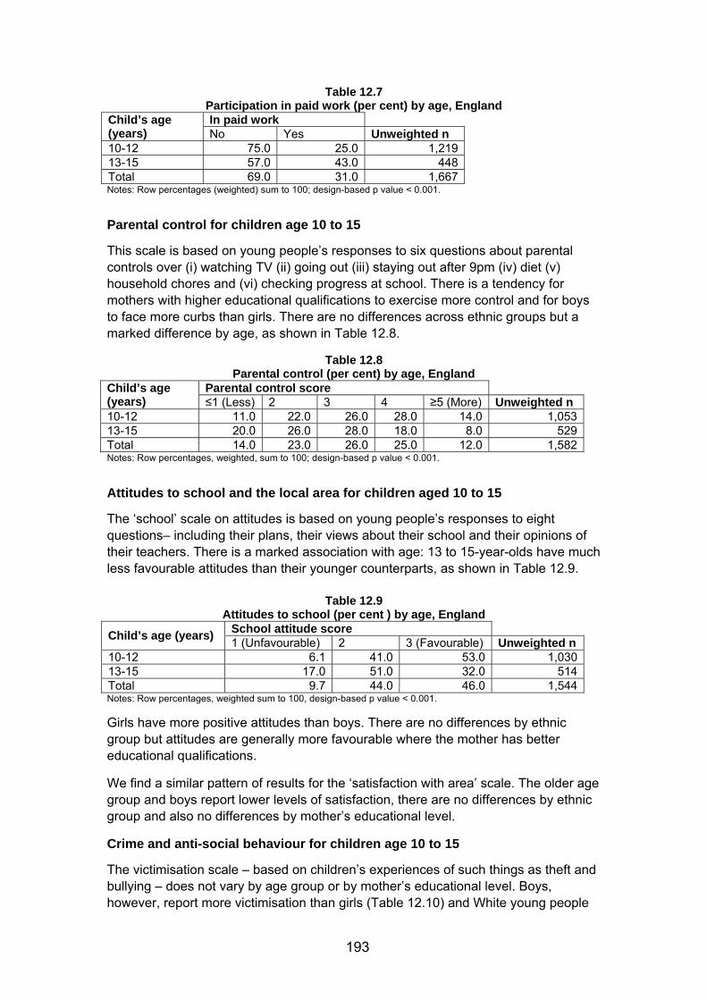
Table 12.7 Participation in paid work (per cent) by age, England In paid work Child’s age
(years) No Yes Unweighted n 10-12 75.0 25.0 1,21913-15 57.0 43.0 448Total 69.0 31.0 1,667Notes: Row percentages (weighted) sum to 100; design-based p value < 0.001. Parental control for children age 10 to 15 This scale is based on young people’s responses to six questions about parental controls over (i) watching TV (ii) going out (iii) staying out after 9pm (iv) diet (v) household chores and (vi) checking progress at school. There is a tendency for mothers with higher educational qualifications to exercise more control and for boys to face more curbs than girls. There are no differences across ethnic groups but a marked difference by age, as shown in Table 12.8.
Table 12.8 Parental control (per cent) by age, England
Parental control score Child’s age (years) ≤1 (Less) 2 3 4 ≥5 (More) Unweighted n 10-12 11.0 22.0 26.0 28.0 14.0 1,053 13-15 20.0 26.0 28.0 18.0 8.0 529 Total 14.0 23.0 26.0 25.0 12.0 1,582 Notes: Row percentages, weighted, sum to 100; design-based p value < 0.001. Attitudes to school and the local area for children aged 10 to 15 The ‘school’ scale on attitudes is based on young people’s responses to eight questions– including their plans, their views about their school and their opinions of their teachers. There is a marked association with age: 13 to 15-year-olds have much less favourable attitudes than their younger counterparts, as shown in Table 12.9.
Table 12.9 Attitudes to school (per cent ) by age, England
School attitude score Child’s age (years) 1 (Unfavourable) 2 3 (Favourable) Unweighted n 10-12 6.1 41.0 53.0 1,030 13-15 17.0 51.0 32.0 514 Total 9.7 44.0 46.0 1,544 Notes: Row percentages, weighted sum to 100, design-based p value < 0.001. Girls have more positive attitudes than boys. There are no differences by ethnic group but attitudes are generally more favourable where the mother has better educational qualifications. We find a similar pattern of results for the ‘satisfaction with area’ scale. The older age group and boys report lower levels of satisfaction, there are no differences by ethnic group and also no differences by mother’s educational level. Crime and anti-social behaviour for children age 10 to 15 The victimisation scale – based on children’s experiences of such things as theft and bullying – does not vary by age group or by mother’s educational level. Boys, however, report more victimisation than girls (Table 12.10) and White young people
193

report more than young people in other ethnic groups, especially the two South Asian groups (Pakistani/Bangladeshi and Indian).
Table 12.10 Victimisation (per cent) by gender England
Victimisation score Child’s sex 0 (None) Some A lot Unweighted n Male 45.0 39.0 16.0 798 Female 53.0 33.0 13.0 848 Total 49.0 36.0 14.0 1,646
Notes: Row percentages, weighted, sum to 100, design-based p value < 0.01. The ‘theft’ scale – based on children’s reports of activities such as shoplifting – shows notably higher rates for the older age group (Table 12.11), somewhat higher rates for boys but no differences by ethnic group and mother’s educational level. The patterns for anti-social behaviour – based on children’s responses to questions involving vandalism or weapons – are similar and the differences between the two age groups are given in Table 12.12.
Table 12.11 Theft (per cent) by age, England
Theft score Child’s age (years) 0 (None) Some A lot Unweighted n 10-12 89.0 8.6 2.1 1,103 13-15 70.0 21.0 8.3 554 Total 83.0 13.0 4.2 1,657
Notes: Row percentages, weighted, sum to 100; design-based p value < 0.001.
Table 12.12 Anti-social behaviour (per cent) by age, England
Anti-social score Child’s age (years) 0 (None) some a lot Unweighted n 10-12 78.0 16.0 6.2 1,109 13-15 64.0 19.0 17.0 555 Total 73.0 17.0 9.8 1,664
Notes: Row percentages, weighted, sum to 100; design-based p value < 0.001.
Conclusion This chapter sets out some of the findings from the older siblings section of MCS2. We see that age is an important explanatory factor for many of the variables considered here but interesting gender and ethnic differences also emerge. The relationship between the experience of these siblings and that of the cohort three-year-olds remains to be explored, along with commonalities and contrasts within families. These responses may prefigure what is in store for their younger brothers and sisters.
References Edwards, A., Barnes, M., Plewis, I. and Morris, K. et al. (2006) Working to Prevent the Social Exclusion of Children and Young People. Research Report 734, London: DfES. National Evaluation of the Children’s Fund (2003) Developing Collaboration in Preventative Services for Children and Young People: First Annual Report, Research Report 528, London: DfES.
194

CONCLUSIONS Kirstine Hansen and Heather Joshi This report draws together descriptive accounts of the different substantive areas covered by the second sweep of the Millennium Cohort Study. It makes no attempt to explore the data exhaustively, nor does it deal in any great detail with the longitudinal link to the first survey. Readers should be aware that there is further material in the dataset that we have not attempted to cover here, such as height, neighbourhood and home observations, and several questions in each topic area. Some sub-groups such as twins and triplets, or children not living with their mothers, have been excluded from many analyses because they require more detailed attention than we can give them at present. We have not included any linkage to geographical datasets or the administrative records from birth registration and maternity hospitals, nor the results of sub-studies such as the survey of mothers who had assisted fertility treatment. What the report does offer is a mainly cross-sectional, broad-brush overview of the dataset, taking covariates one at a time. It also highlights possible topics and relationships likely to interest policy-makers, academics and wider society. By offering a cross-sectional framework upon which further analysis may hang, it aims to encourage the further exploration of such relationships by external MCS users as well as ourselves. Part of the role of the Centre for Longitudinal Studies is to develop and provide research resources for others as well as carrying out our own studies. Some of the findings reported here will be examined in greater detail by CLS staff and MCS collaborators in a further book in the Children of the 21st Century series, to be published early in 2008. The main findings are outlined in our Executive Summary, and highlights of chapters 2-11, with some graphical illustrations, can be found in briefing papers also available on the CLS website (www.cls.ioe.ac.uk). The Children of the New Century had reached the age of three by the time of this survey. Virtually all had long since learned to walk, and all but a few (around one in ten) were talking with at least an adequate vocabulary for their age. A large proportion had also reached school readiness standards, and many were attending early-education settings. A few were not yet toilet-trained, and a small minority had serious behavioural problems or poor health. This report does not reveal whether these problems are experienced by the same individuals. It does show that there are patterns along gender and social lines but it is also clear from our research that a child’s progress is not solely dependent on these factors. Every child is different. Of the three social factors on which the survey design focused, ethnicity is one where there is much multi-directional diversity in the results reported here. The non-White groups are far from homogeneous, and different groups appear to do well or badly on different counts. On economic disadvantage, at the level of community and the individual family, there are signs that parents’ circumstances are being reflected in
195

the development of children as young as three. However, though disadvantages are associated with poorer outcomes, this is no more than a raised risk. Many children in 195 difficult circumstances were doing well, and the causal pathways, if any, have not been investigated. The third feature of the survey design was to permit comparisons between and within the four countries of the UK. In general, the differences between countries were modest. Different attitudes in Northern Ireland to children acquiring religious values were not surprising. Lower poverty rates and higher cognitive scores for children in Scotland are, however, intriguing and cry out for further investigation, as does most of the material in this report. It should be apparent from this report and these summaries that the MCS is already a very rich source of information with great potential to contribute to policy and scientific uses. This report is one building block in the process of realising this potential. The newly longitudinal dataset monitors the circumstances of children as they grow up. As this report has shown, MCS data collected as early as age three allow us to examine a range of child outcomes such as health, growth, cognitive ability and behaviour. At the same time, they provide an extensive collection of explanatory variables including family, environmental and individual factors which help to analyse differences in outcomes. This first set of measurements of physical, cognitive and behavioural development of a national cohort of children in their early years is already showing that, despite unprecedented policy initiatives to support young children and their families and to eliminate child poverty, there is still evidence of economic and ethnic disadvantages for three-year-olds. Whether these inequalities would have been greater without the policy interventions and whether they are greater than those charted in previous birth cohort studies are questions left to the further research this report is designed to facilitate. The range of both outcomes and explanatory data available will expand as the MCS children grow older and the survey collects more information. The outcomes at age three will in turn become the variables that affect future development. Data on the children at age five will become available in late 2007 (assuming a less problematic transition from field to archive than for this sweep), around the same time as the survey at age seven begins. As well as the research potential of further follow-ups in the MCS, there are already possibilities for comparing previous studies. This is beyond the scope of this document, but it is hoped that readers will find much to interest them within its terms of reference and that it will inspire some to take the next steps.
196